Zeroth-order Stochastic Cubic Newton Method with Low-rank Hessian Estimation

Abstract

This paper focuses on the problem of minimizing a finite-sum loss $\frac{1}{N}$ $\sum_{\xi=1}^{N}f(\mathbf{x};\xi)$, where only function evaluations of $f(\cdot;\xi)$ is allowed. For a fixed $\xi$, which represents a (batch of) training data, the Hessian matrix $\nabla^{2}f(\mathbf{x};\xi)$ is usually low-rank. We develop a stochastic zeroth-order cubic Newton method for such problems, and prove its efficiency. More specifically, we show that when $\nabla^{2}f(\mathbf{x};\xi)\in\mathbb{R}^{n\times n}$ is of rank-$r$, $\mathcal{O}\left(\frac{n}{\eta^{\frac{7}{2}}}\right)+\widetilde{\mathcal{O}}\left(\frac{n^{2}r^{2}}{\eta^{\frac{5}{2}}}\right)$ function evaluations guarantee a second order $\eta$-stationary point with high probability. This result improves the dependence on dimensionality compared to the existing state-of-the-art. This improvement is achieved via a new Hessian estimation method, which can be efficiently computed by finite-difference operations, and does not require any incoherence assumptions. Numerical experiments are provided to demonstrate the effectiveness of our algorithm.

1 Introduction

Optimization plays a crucial role in machine learning, statistics, and related fields. Often times in practice, the objective function has no analytical formula, has a too complicated formula, or has to be private (El Mestari et al.,, 2024, and references therein). In such scenarios, the significance of zeroth-order optimization becomes evident, as it provides an effective alternative that relies solely on function evaluations. To this end, we study zeroth-order stochastic optimization problems. More specifically, we focus on solving the following problem

$$\min_{\mathbf{x}\in\mathbb{R}^{n}}F(\mathbf{x}):=\int_{\xi\in\Theta}f(\mathbf{x};\xi)\mu(d\xi),$$ (1)

where only function evaluations of $f(\cdot;\xi)$ is allowed. Here $\mu$ is a distribution over the set $\Theta$.

The efficiency of a zeroth-order optimization algorithm is primarily judged by sample complexity: the number of function evaluations required to achieve a certain level of accuracy. Recently, compressed sensing techniques have been introduced to the field of zeroth-order optimization (Wang et al.,, 2018; Cai et al., 2022a, ; Cai et al., 2022b, ), so that the sample complexity of zeroth-order optimization methods can be greatly reduced for functions with sparse or compressible gradient. Yet gradient information alone is insufficient in several important scenarios. In particular, zeroth-order optimization often deals with complex function landscapes where first-order methods may become trapped in saddle points or local minima.

This motivates the adaptation of second-order methods to zeroth-order optimization scenarios, aiming to use curvature information to accelerate convergence and avoid saddle points. The primary challenge is efficiently obtaining an estimator for the Hessian matrix $\nabla^{2}f(\mathbf{x};\xi)$. Existing Hessian estimation methods (e.g., Balasubramanian and Ghadimi,, 2022; Feng and Wang,, 2023) is overly conservative for low-rank Hessians $\nabla^{2}f(\mathbf{x};\xi)$, which is prevalent in stochastic optimization.

(M) Consider the classic task of logistic regression, which lays a foundation for neural network classification. For logistic regression, the objective function (1) is the logistic loss

$$F(\mathbf{x}):=\frac{1}{N}\sum_{\xi=1}^{N}f(\mathbf{x};\xi),\qquad f(\mathbf{x};\xi)=\log\left(1+e^{-y_{\xi}\mathbf{z}_{\xi}^{\top}\mathbf{x}}\right)$$ (2)

where $\left(\mathbf{z}_{\xi},y_{\xi}\right)$ ($y_{\xi}\in\{-1,+1\}$) is the feature and label of the $\xi$-th training data; The overall loss of the logistic regression $F$ may well have a full-rank Hessian. However, for each data point indexed by $\xi$, the loss function $f(\mathbf{x};\xi)$ admits a rank-1 Hessian at any $\mathbf{x}$. In the language of this paper, such phenomenon corresponds to $\nabla^{2}f(\mathbf{x};\xi)$ being low-rank for all $\mathbf{x}\in\mathbb{R}^{n}$ and $\xi\in\Theta$.

To this end, we propose a low-rank Hessian estimator with high probability guarantee and apply it to zeroth-order Newton optimization. In this work, we aim to demonstrate that, by leveraging the low-rank assumption and employing the proposed estimator, achieving equivalent accuracy requires fewer finite-difference computations, highlighting the efficiency gains afforded by incorporating low-rank structures in Hessian estimation.

1.1 Low-rank Hessian Estimation

A primer step for Newton-type zeroth-order method is Hessian estimation. In recent years, the rise of large models and big data has posed the high-dimensionality of objective functions as a primary challenge in finite-difference Hessian estimation. To address this, high-dimensional Hessian estimators, like (Balasubramanian and Ghadimi,, 2021; Wang,, 2023; Feng and Wang,, 2023; Li et al.,, 2023), have emerged to reduce the required number of function value samples.

However, existing methods tends to be overly conservative when the Hessian matrix is low-rank, which is prevalent in modern scenarios. For the optimization problem (1), it is very common that the Hessian of $f(\cdot;\xi)$ is low-rank for any fixed $\xi$. For example, if (1) is the training loss of a standard logistic regression and each $\xi$ corresponds to a training data point, then $\nabla^{2}f(\cdot;\xi)$ is low-rank for each $\xi$, as discussed in (M).

To fill in the gap, in this work, we develop an efficient finite-difference Hessian estimation method for low-rank Hessian via matrix recovery. While a substantial number of literature studies the sample complexity of low-rank matrix recovery, we emphasize that none of them are directly applicable to our scenario. This is either due to the overly restrictive global incoherence assumption (See Remark 1 and Figure 1) or a prohibitively large number of finite-difference computations, as we discuss in detail in section 1.3.2. We prove that without the incoherence assumption, for an $n\times n$ Hessian matrix with rank $r$, we can exactly recover the matrix with high probability from $\mathcal{O}(nr^{2}\log^{2}n)$ proper zeroth-order finite-difference computations.

In order to reconstruct a low-rank Hessian matrix $H$ of size $n\times n$ using $\ll n^{2}$ finite-difference operations, it is essential to obtain a matrix measurement of the underlying matrix $H$. A matrix measurement involves performing a matrix multiplication or Frobenius inner product between the hidden matrix $H$ and some measurement matrices $A$’s that we select. With these matrix measurements in place, we use the following trace norm minimization approach (Fazel,, 2002; Recht et al.,, 2010; Candès and Tao,, 2010; Gross,, 2011; Candes and Recht,, 2012):

$$\min_{\widehat{H}\in\mathbb{R}^{n\times n}}\|\widehat{H}\|_{1},\quad\text{ subject to }\quad\mathcal{S}\widehat{H}=\mathcal{S}H,$$ (3)

where $\mathcal{S}:=\frac{1}{M}\sum_{i=1}^{M}\mathcal{P}_{i}$ and $\mathcal{P}_{i}$ is a matrix measurement operation that can be obtained via $\mathcal{O}(1)$ finite-difference computations. For our problem, it is worth emphasizing that the operator $\mathcal{P}_{i}$ used in this paper has two properties.

• (R1) $\mathcal{P}_{i}$ is different from the measurement operation used for matrix completion. Otherwise an incoherence assumption is needed; See Remark 1 in Section 1.3.2 for more details.

• (R2) $\mathcal{P}_{i}$ cannot involve the inner product between the Hessian matrix and a general matrix, since this operation cannot be efficiently obtained through finite-difference computations. See Remark 2 in Section 1.3.2 for more details.

Due to the above two requirements, existing theory for matrix recovery fails to provide satisfactory guarantees for low-rank Hessian estimation. In this paper, we show that without the incoherence assumption, for an $n\times n$ Hessian matrix with rank $r$, we can exactly recover the matrix with high probability from $\mathcal{O}(nr^{2}\log^{2}n)$ proper zeroth-order finite-difference computations.

1.2 Convergence Results

Based on our low-rank Hessian estimation, we design stochastic zeroth-order cubic Newton method for smooth programs. In particular, we prove the following results for real-valued functions defined over $\mathbb{R}^{n}$.

• When the rank of the Hessian is bounded by $r$, $\mathcal{O}\left(\frac{n}{\eta^{\frac{7}{2}}}\right)+\widetilde{\mathcal{O}}\left(\frac{n^{2}r^{2}}{\eta^{\frac{5}{2}}}\right)$ function evaluations guarantee a second order $\eta$-stationary point in the expectation sense; See Theorem 3 and Definition 1 for details.

Our results offer a significant reduction in function evaluation complexity compared to the previous work of Balasubramanian and Ghadimi, (2022), which has a function evaluation complexity of $\mathcal{O}\left(\frac{n}{\eta^{\frac{7}{2}}}\right)+\widetilde{\mathcal{O}}\left(\frac{n^{4}}{\eta^{\frac{5}{2}}}\right)$ for a second order $\eta$-stationary point in the expectation sense. This reduction is particularly beneficial when dealing with the low-rank Hessian structure, which is ubiquitous as discussed in (M).

1.3 Prior Arts

A significant portion of the optimization literature is dedicated to studying zeroth-order optimization (or derivative-free optimization) methods (e.g., Conn et al.,, 2009; Shahriari et al.,, 2015). Among many zeroth order optimization mechanisms, a classic and prosperous line of works focuses on estimating gradient/Hessian using zeroth order information and use the estimated gradient/Hessian for downstream optimization algorithms.

1.3.1 Zeroth-order Optimization

In recent decades, due to lack of direct access to gradients in real-world applications, zeroth order optimization has attracted the attention of many researchers (Flaxman et al.,, 2005; Ghadimi and Lan,, 2013; Duchi et al.,, 2015; Nesterov and Spokoiny,, 2017; Chen et al.,, 2017; Liu et al.,, 2018; Wang et al.,, 2018; Chen et al.,, 2019; Tu et al.,, 2019; Liu et al.,, 2020; Balasubramanian and Ghadimi,, 2021; Li et al.,, 2022; Cai et al., 2022a, ; Cai et al., 2022b, ; Hare et al.,, 2023). In particular, Flaxman et al., (2005) introduced the single-point gradient estimator for the purpose of bandit learning. Afterwards, many modern gradient/Hessian estimators have been introduced and subsequent zeroth order optimization algorithms have been studied. To name a few, Duchi et al., (2015); Nesterov and Spokoiny, (2017) have studied zeroth order optimization algorithm for convex objective and established in expectation convergence rates. Replacing the exact gradient by a gradient estimator, many widely used first-order methods now have their zeroth-order counterparts, including ZO-SGD (Ghadimi and Lan,, 2013), ZO-SVRG (Liu et al.,, 2018) and ZO-adam (Chen et al.,, 2019), just to name a few.

A line of research utilizes the principles of compressed sensing to zeroth-order optimization (Bandeira et al.,, 2012; Wang et al.,, 2018; Cai et al., 2022a, ; Cai et al., 2022b, ). More specifically, Cai et al., 2022a used one-bit compressed sensing for gradient estimation, and Cai et al., 2022b used CoSaMP (Needell and Tropp,, 2009) to estimate compressible gradients, which leads to significantly reduced sample complexity for functions with compressible gradients.

Parallel to the methods mentioned above, there are various other zeroth-order methods (e.g., Rios and Sahinidis,, 2013). One line of investigation focuses on interpolating the objective using polynomials. For instance, Conn et al., 2008a studied the interpolation approach for derivative-free optimization, and provided a bound on the Hessian of the interpolation and the true objective. Along the same line, Conn et al., 2008b studied the interpolation method for derivative free optimization in the over- and under-determined case. Based on principles of compressed sensing, Bandeira et al., (2012) investigated the interpolation approach under sparsity assumptions.

Perhaps the most related prior art is Balasubramanian and Ghadimi, (2021), where Stein’s identity is used for Hessian estimators and this Stein-type Hessian estimator is applied to cubic regularized Newton’s method (Nesterov and Polyak,, 2006). However, the methods of Balasubramanian and Ghadimi, (2021) can lead to overly conservative sample complexity, due to a sub-optimal estimator for low-rank Hessians. In this paper, we close this gap by introducing a new Hessian estimator.

1.3.2 Hessian Estimation

Perhaps the history of zeroth-order Hessian estimation can date back to Newton’s time, when finite-difference principles were used to approximate derivatives (Taylor,, 1715). In recent years, researchers from various fields have contributed to this topic (e.g., Broyden et al.,, 1973; Fletcher,, 2000; Spall,, 2000; Balasubramanian and Ghadimi,, 2021; Li et al.,, 2023).

In quasi-Newton-type methods (e.g., Goldfarb,, 1970; Shanno,, 1970; Broyden et al.,, 1973; Ren-Pu and Powell,, 1983; Davidon,, 1991; Fletcher,, 2000; Spall,, 2000; Xu and Zhang,, 2001; Rodomanov and Nesterov,, 2022), gradient-based Hessian estimators were used for iterative optimization algorithms. Based on the Stein’s identity (Stein,, 1981), Balasubramanian and Ghadimi, (2021) introduced a Hessian estimator, and combined it with cubic regularized Newton’s method (Nesterov and Polyak,, 2006) for non-convex optimization. Li et al., (2023) generalizes the Stein-type Hessian estimators to Riemannian manifolds. Parallel to (Balasubramanian and Ghadimi,, 2021; Li et al.,, 2023), Wang, (2023); Feng and Wang, (2023) investigated the Hessian estimator that inspires the current work.

Also, some recent studies presented a new direction for derivative estimation. Hare et al., (2023) introduced a matrix algebra method for estimating Hessians using function evaluations, and considered a “partial Hessian” case. Expanding on this line of research, Jarry-Bolduc and Planiden, (2023) extends the principle of Hare et al., (2023) to estimate derivatives of even higher orders.

Yet prior to our work, no methods from the zeroth-order Hessian estimation community focuses on low-rank Hessian estimation. To this end, we propose a low-rank Hessian estimator that simultaneously satisfy (R1) and (R2), which also adds to the literature of matrix recovery, since existing matrix recovery methods either requires an incoherence assumption (referred to as matrix completion-type methods, violates (R1)) (Fazel,, 2002; Cai et al.,, 2010; Candes and Plan,, 2010; Candès and Tao,, 2010; Keshavan et al.,, 2010; Lee and Bresler,, 2010; Fornasier et al.,, 2011; Gross,, 2011; Recht,, 2011; Candes and Recht,, 2012; Hu et al.,, 2012; Mohan and Fazel,, 2012; Negahban and Wainwright,, 2012; Wen et al.,, 2012; Vandereycken,, 2013; Wang et al.,, 2014; Chen,, 2015; Tanner and Wei,, 2016; Gotoh et al.,, 2018; Chen et al.,, 2020; Ahn et al.,, 2023), or cannot be efficiently computed by finite-difference operations (referred to as matrix regression-type methods, violates (R2)) (Tan et al.,, 2011; Eldar et al.,, 2012; Chandrasekaran et al.,, 2012; Rong et al.,, 2021; Rohde and Tsybakov,, 2011; Fan et al.,, 2021; Xiaojun Mao and Wong,, 2019).

Remark 1.

Incoherence is a common assumption in matrix completion literature. It requires that there is a nontrivial angle between the singular space of the desired low-rank matrix and the observation basis. For example, if the observation basis is the canonical basis $\mathbf{e}_{i}$ and the right singular space is the span of $\psi_{1},\cdots,\psi_{r}$, incoherence requires $\max_{i,j}|\mathbf{e}_{i}^{\top}\psi_{j}|$ to be small. The intuition is that if the first row of the desired matrix aligns exactly with the observation basis, and all other rows are zero, the matrix cannot be recovered unless all of its entries are observed. In the context of optimization, when applying matrix completion methods based on the incoherence assumption, we need to assume that such an angle holds uniformly for the Hessian matrix at any given point $\mathbf{x}$. This is overly restrictive, as illustrated in Figure 1.

Remark 2.

For matrix regression-type methods, we observe the inner product of the target matrix $H$ with a set of measurement matrices $A_{1},A_{2},\cdots,A_{M}$. Specifically, we have the observation $\left<H,A_{i}\right>:=\mathrm{tr}(H^{*}A_{i})$ and our goal is to recover $H$. Despite the elegant results in matrix recovery using linear measurements, they are not directly applicable to Hessian estimation tasks. This limitation arises from the fact that a general linear measurement cannot be efficiently approximated by a zeroth-order estimation. To further illustrate this fact, let us consider the Taylor approximation, which, by the fundamental theorem of calculus, is the foundation for zeroth-order estimation. In the Taylor approximation of $f$ at $\mathbf{x}$, the Hessian matrix $\nabla^{2}f(\mathbf{x})$ will always appear as a bilinear form. Therefore, a linear measurement $\left<A,\nabla^{2}f(\mathbf{x})\right>$ for a general $A$ cannot be included in a Taylor approximation of $f$ at $\mathbf{x}$. In the language of optimization and numerical analysis, for a general measurement matrix $A$, one linear measurement $\left<A,H\right>$ may require far more than $\mathcal{O}(1)$ finite-difference computations. Consequently, the theory providing guarantees for linear measurements does not extend to zeroth-order Hessian estimation.

Figure 1: Incoherence condition for $\nabla^{2}f(\mathbf{x})$ at multiple points. Let $\psi(A)$ be the singular vector of matrix $A$ whose span has the smallest angle with canonical basis (e.g. $\mathbf{e}_{1}$). The sampling complexity to recover $A$ is higher if the angle is smaller. In the left subfigure, the sample complexity to guarantee the recovery of $\nabla^{2}f(\mathbf{x}_{1})$ depends on $\alpha$, which is an angle determined by the Hessian at $\mathbf{x}_{1}$ and the canonical basis. In the right subfigure, the sample complexity to guarantee the recovery of both $\nabla^{2}f(\mathbf{x}_{1})$ and $\nabla^{2}f(\mathbf{x}_{2})$ depends on a smaller angle $\beta\leq\alpha$. To recover the $\nabla^{2}f(\mathbf{x})$ at all $\mathbf{x}$ with a fixed number of sampling, a uniform smallest angle is required for all $\mathbf{x}$, which is overly restrictive.

1.4 Summary of Contributions

To sum up, this paper focuses on the important problem of zeroth-order stochastic optimization where the Hessian on a batch of training data is low-rank; See paragraph (M). We focus on second-order methods for such problems, and our main contributions are as follows.

1. We propose a Hessian estimation method for low-rank Hessians based on matrix recovery principles. Notably, our method does not require any incoherence assumptions, and can be efficiently computed via finite-difference operations. Specifically, we prove that, with high probability, a rank-$r$ Hessian matrix of size $n\times n$ can be accurately approximated using $\widetilde{\mathcal{O}}(nr^{2})$ finite-difference operations.

2. Based on our Hessian estimation method, we introduce a variation of the stochastic zeroth-order cubic Newton method that takes advantage of the low-rank structure of the Hessian on a batch of training data. This new version improves the sample complexity of the existing state-of-the-art zeroth-order stochastic cubic Newton method. In particular, when the rank of the Hessian is bounded by $r$, our method guarantees a second-order $\eta$-stationary point with $\mathcal{O}\left(\frac{n}{\eta^{\frac{7}{2}}}\right)+\widetilde{\mathcal{O}}\left(\frac{n^{2}r^{2}}{\eta^{\frac{5}{2}}}\right)$ function evaluations. This is an improvement over the current state-of-the-art sample complexity of $\mathcal{O}\left(\frac{n}{\eta^{\frac{7}{2}}}\right)+\widetilde{\mathcal{O}}\left(\frac{n^{4}}{\eta^{\frac{5}{2}}}\right)$ for finding a second-order $\eta$-stationary point using stochastic zeroth-order cubic Newton.

1.5 Notations and Conventions

Before proceeding further, we list some notations and conventions that will be used throughout the paper. First of all, we agree on the following notations for matrix norms.

• $\|\cdot\|$, $\|\cdot\|_{op}$ denote the operator norm (Schatten $\infty$-norm);

• $\|\cdot\|_{2}$, $\|\cdot\|_{F}$ denote the Frobenius norm (Schatten $2$-norm);

• $\|\cdot\|_{1}$ is the trace norm (Schatten $1$-norm, nuclear norm).

Also, the notation $\|\cdot\|$ is overloaded for vector norm and tensor norm. For a vector $\mathbf{v}\in\mathbb{R}^{n}$, $\|\cdot\|$ is its Euclidean norm; For a tensor $V\in\left(\mathbb{R}^{n}\right)^{\otimes p}$ ($p\geq 2$), $\|\cdot\|$ is its Schatten $\infty$-norm. For any matrix $A$ with singular value decomposition $A=U\Sigma V^{\top}$, we define $\mathrm{sign}(A)=U\mathrm{sign}(\Sigma)V^{\top}$ where $\mathrm{sign}(\Sigma)$ applies a $\mathrm{sign}$ function to each entry of $\Sigma$. Also, for any real matrix $A$, we define $|A|$ to be the entry-wise absolute value of the matrix $A$.

For a vector $\mathbf{u}=\left(u_{1},u_{2},\cdots,u_{n}\right)^{\top}\in\mathbb{R}^{n}$ and a positive number $r\leq n$, we define notations

$$\mathbf{u}_{:r}=\left(u_{1},u_{2},\cdots,u_{r},0,0,\cdots,0\right)^{\top}\;\text{and}\;\mathbf{u}_{r:}=\left(0,0,\cdots,0,u_{r},u_{r+1},\cdots,u_{n}\right)^{\top}.$$

The following assumptions appear frequently in our analysis.

Assumption 1.

The Hessian is Lipschitz continuous, i.e., there exists $L_{2}>0$ such that for any $\mathbf{x},\mathbf{y}\in\mathbb{R}^{d}$ and any $\xi\in\Theta$,

$$\|\nabla^{2}f(\mathbf{x};\xi)-\nabla^{2}f(\mathbf{y};\xi)\|\leq L_{2}\|\mathbf{x}-\mathbf{y}\|.$$

where $\|\cdot\|$ denotes spectral norm for matrices and $2$-norm for vectors.

Assumption 2.

There exists $r\ll n$, such that For any $\mathbf{x}\in\mathbb{R}^{n}$ and any $\xi\in\Theta$, $rank(\nabla^{2}f(\mathbf{x};\xi))\leq r$.

Also, we use $C$ and $c$ to denote unimportant absolute constants. The numbers $C$ and $c$ may or may not take the same value at each occurrence. We use $K$’s ($K,K_{1},K_{2},$ etc.) to denote constants whose value will be held fixed throughout. A detailed table of notations is in the Appendix.

Paper Organization. The rest of the paper is structured as follows: Section 2 presents a summary of the main findings and outlines the algorithm procedure, encompassing both the method for estimating the Hessian and the downstream stochastic cubic Newton method. Theoretical guarantees for the Hessian estimation method are then provided in Section 3. In Section 4, an analysis of the primary algorithm is presented, highlighting the utilization of the low-rank structure of the Hessian to reduce the sample complexity of the stochastic zeroth-order cubic Newton method. Section 5 focuses on experimental investigations. This section includes empirical results for matrix recovery guarantee and convergence results for the stochastic cubic Newton method that employs a low-rank Hessian estimation method. Finally, we conclude the paper in Section 6.

2 The Algorithm Procedure and Main Results

Many widely used zeroth-order algorithms borrow from derivative-based methods, by estimating the derivatives first. As is well-known, second-order information can better capture the curvature of the objective, and thus accelerate the convergence rate. To this end, we study the zeroth-order stochastic cubic Newton method, whose algorithmic framework is summarized in Algorithm 1.

Algorithm 1 High-level description of zeroth-order cubic Newton method

1:Goal. A finite-sum-type objective $\int_{\xi\in\Theta}f(\mathbf{x};\xi)\mu(d\xi)$.

2:Input parameters. $T$, $m_{1}$, $m_{2}$. /* $T$ is the total time horizon; $m_{1}$ (resp. $m_{2}$) describes number of function evaluations used for gradient (resp. Hessian) estimation at each step.  */

3:/* There are additional input parameters, as we will detail in subsequent sections. */

4:Initialize. $\mathbf{x}_{0}\in\mathbb{R}^{n}$.

5:for $t=0,1,2,\cdots,T$ do

6:   Generate $iid$ $\{\xi_{t}^{i,1}\}_{i\in[m_{1}]}$ following $\mu$. Obtain gradient estimator $\mathbf{g}_{t}$ for ${\nabla}F(\mathbf{x}_{t})$, using function evaluations for $\{f(\mathbf{x}_{t};\xi_{t}^{i,1})\}_{i\in[m_{1}]}$.

7:   Generate $iid$ $\{\xi_{t}^{i,2}\}_{i\in[m_{2}]}$ following $\mu$. Obtain Hessian estimator $\widehat{H}_{t}$ for ${\nabla}^{2}F(\mathbf{x}_{t})$, using function evaluations for $\{f(\mathbf{x}_{t};\xi_{t}^{i,2})\}_{i\in[m_{2}]}$.

8:   Perform a cubic Newton step with estimated gradient and Hessian, and obtain $\mathbf{x}_{t+1}$.

9:end for

The cubic Newton method is due to (Nesterov and Polyak,, 2006; Nesterov,, 2008), and the algorithmic framework in Algorithm 1 was proposed by (Balasubramanian and Ghadimi,, 2022). However, several important questions remain unanswered:

What is the sample complexity for Hessian estimation for low-rank Hessian matrices? How does this sample complexity affect the overall convergence performance of the algorithm?

To answer these important questions, we start with a Hessian estimation method designated to low-rank Hessians.

2.1 Low-rank Hessian Estimation

We start with a finite-difference scheme that can be viewed as a matrix measurement operation. In stochastic zeroth-order optimization, a $\xi$ is randomly selected at each step, and function evaluations of $f(\cdot;\xi)$ is performed. Once a $\xi$ is selected, the function $f(\cdot;\xi)$ is fixed. Throughout this subsection, we will omit the explicit mention of $\xi$ and refer to $f(\cdot;\xi)$ as simply $f(\cdot)$ when there is no confusion. The Hessian of a function $f:\mathbb{R}^{n}\to\mathbb{R}$ at a given point $\mathbf{x}$ can be estimated as follows (Wang,, 2023; Feng and Wang,, 2023)

$$\widehat{\nabla}_{\mathbf{u},\mathbf{v},\delta}^{2}f(\mathbf{x}):=$$

$$n^{2}\frac{f(\mathbf{x}+\delta\mathbf{v}+\delta\mathbf{u})-f(\mathbf{x}-\delta\mathbf{v}+\delta\mathbf{u})-f(\mathbf{x}+\delta\mathbf{v}-\delta\mathbf{u})+f(\mathbf{x}-\delta\mathbf{v}-\delta\mathbf{u})}{4\delta^{2}}\mathbf{u}\mathbf{v}^{\top},$$ (4)

where $\delta$ is the finite-difference granularity, and $\mathbf{u},\mathbf{v}$ are finite-difference directions. Difference choices of laws of $\mathbf{u}$ and $\mathbf{v}$ leads to different Hessian estimators. For example, $\mathbf{u},\mathbf{v}$ can be independent vectors uniformly distributed over the canonical basis $\{\mathbf{e}_{1},\mathbf{e}_{2},\cdots,\mathbf{e}_{n}\}$, or uniformly distributed over the unit sphere.

We first show that the finite difference Hessian estimator (4) is approximately a matrix measurement, in Proposition 1 and Lemma 1.

Proposition 1.

Consider an estimator defined in (4). Let the underlying function $f$ be three-time continuously differentiable. Let $\mathbf{u},\mathbf{v}\in\mathbb{R}^{n}$ be two random vectors. Then for any fixed $\mathbf{x}\in\mathbb{R}^{n}$,

$$\widehat{\nabla}_{\mathbf{u},\mathbf{v},\delta}^{2}f(\mathbf{x})\to n^{2}\mathbf{u}\mathbf{u}^{\top}\nabla^{2}f(\mathbf{x})\mathbf{v}\mathbf{v}^{\top},\;\;a.s.$$

as $\delta\to 0_{+}$.

Proof.

Let $\left(\Omega,\mathcal{F},\mu\right)$ be the probability space over which $\mathbf{u},\mathbf{v}$ are defined. Let $\omega\in\Omega$ be any element in the sample space of the random vectors $\mathbf{u},\mathbf{v}$. By Taylor’s Theorem and that the Hessian matrix is symmetric, we have

$$\;\widehat{\nabla}_{\mathbf{u}(\omega),\mathbf{v}(\omega),\delta}^{2}f(\mathbf{x})$$

$$= \;\frac{n^{2}}{4}\left(\mathbf{v}(\omega)+\mathbf{u}(\omega)\right)^{\top}\nabla^{2}f(\mathbf{x})\left(\mathbf{v}(\omega)+\mathbf{u}(\omega)\right)\mathbf{u}(\omega)\mathbf{v}(\omega)^{\top}$$

$$-\left(\mathbf{v}(\omega)-\mathbf{u}(\omega)\right)^{\top}\nabla^{2}f(\mathbf{x})\left(\mathbf{v}(\omega)-\mathbf{u}(\omega)\right)\mathbf{u}(\omega)\mathbf{v}(\omega)^{\top}$$

$$+\mathcal{O}\left(\delta\left(\|\mathbf{v}(\omega)\|+\|\mathbf{u}(\omega)\|\right)^{3}\right)$$

$$= \;n^{2}\mathbf{u}(\omega)^{\top}\nabla^{2}f(\mathbf{x})\mathbf{v}(\omega)\mathbf{u}(\omega)\mathbf{v}(\omega)^{\top}+\mathcal{O}\left(\delta\left(\|\mathbf{v}(\omega)\|+\|\mathbf{u}(\omega)\|\right)^{3}\right)$$

$$= \;n^{2}\mathbf{u}(\omega)\mathbf{u}(\omega)^{\top}\nabla^{2}f(\mathbf{x})\mathbf{v}(\omega)\mathbf{v}(\omega)^{\top}+\mathcal{O}\left(\delta\left(\|\mathbf{v}(\omega)\|+\|\mathbf{u}(\omega)\|\right)^{3}\right),$$

where the last equality uses that $\mathbf{u}(\omega)^{\top}\nabla^{2}f(\mathbf{x})\mathbf{v}(\omega)$ is a real number and can thus be moved around as a whole.

As $\delta\to 0_{+}$, the estimator (4) converges to $n^{2}\mathbf{u}(\omega)\mathbf{u}(\omega)^{\top}\nabla^{2}f(\mathbf{x})\mathbf{v}(\omega)\mathbf{v}^{\top}(\omega)$ for any sample point $\omega$. This concludes the proof.

∎

When the finite-difference granularity is non-vanishing, we have the following lemma that quantifies the measurement error, whose proof can be found in Section 3.

Lemma 1.

Let $f$ have $L_{2}$-Lipschitz Hessian: $\|\nabla^{2}f(\mathbf{x})-\nabla^{2}f(\mathbf{y})\|\leq L_{2}\|\mathbf{x}-\mathbf{y}\|$, for all $\mathbf{x},\mathbf{y}\in\mathbb{R}^{n}$. Consider the estimator defined in (4). Let $M<\frac{n(n+1)}{2}$.  For each $\mathbf{x}\in\mathbb{R}^{n}$, there exists a real symmetric random matrix $H$ of size $n\times n$ such that (i) $H$ is determined by $\{\mathbf{u}_{i},\mathbf{v}_{i}\}_{i=1}^{M}$, and (ii) $\|H-\nabla^{2}f(\mathbf{x})\|{\leq}4L_{2}\delta$ almost surely, and (iii)

$$\widehat{\nabla}_{\mathbf{u}_{i},\mathbf{v}_{i},\delta}^{2}f(\mathbf{x})={n^{2}}\mathbf{u}_{i}\mathbf{u}_{i}^{\top}H\mathbf{v}_{i}\mathbf{v}_{i}^{\top},\quad i=1,2,\cdots,M,$$

where $\mathbf{u}_{i},\mathbf{v}_{i}\overset{iid}{\sim}\text{Unif}(\mathbb{S}^{n-1})$.

With Proposition 1 and Lemma 1 in place, we can formulate Hessian estimation task as a matrix recovery problem. Specifically, the Hessian estimation seeks to solve the following convex program

$$\min_{\widehat{H}\in\mathbb{R}^{n\times n}}\|\widehat{H}\|_{1},\text{ subject to }\mathcal{S}\widehat{H}=\frac{1}{M}\sum_{i=1}^{M}\widehat{\nabla}_{\mathbf{u}_{i},\mathbf{v}_{i},\delta}f(\mathbf{x})=\frac{1}{M}\sum_{i=1}^{M}n^{2}\mathbf{u}_{i}\mathbf{u}_{i}^{\top}H\mathbf{v}_{i}\mathbf{v}_{i}^{\top},$$ (5)

where $\|\cdot\|_{1}$ denotes trace norm, $\mathbf{u}_{i},\mathbf{v}_{i}\overset{iid}{\sim}\mathrm{Unif}(\mathbb{S}^{n-1})(i=1,\cdots,M)$ are sampled uniformly from the unit sphere, $\mathcal{S}:=\frac{1}{M}\sum_{i=1}^{M}\mathcal{P}_{i}$ with

$$\mathcal{P}_{i}A=n^{2}\mathbf{u}_{i}\mathbf{u}_{i}^{\top}A\mathbf{v}_{i}\mathbf{v}_{i}^{\top}$$ (6)

for any $A\in\mathbb{R}^{n\times n}$, and $H$ is a random symmetric matrix determined by $\{\mathbf{u}_{i},\mathbf{v}_{i}\}_{i=1}^{M}$ that is implicitly obtained via Eq. 4 (See Lemma 1).

Remark 3.

Before proceeding any further, let’s take a moment to establish some consistent terminology that will be used throughout the rest of the paper. From here on, we will refer to a matrix measurement as the operation $\mathcal{P}_{i}$ in (6). The number of matrix measurements will also be referred to as the number of samples. As demonstrated in Eq. 4 and Lemma 1, a single matrix measurement can be estimated using $4$ function evaluations, up to any precision.

Hence, by combining terminologies from both matrix completion and optimization, we can say that the efficiency of a Hessian estimator is measured by the number of function evaluations, or by number of samples/matrix measurements. Recall that the number of measurements equals the number of function evaluations up to a multiplicative constant $4$.

The above Hessian estimator is guaranteed to output a high accuracy estimator with high probability. More specifically, the Hessian estimator satisfies the following theorem:

Theorem 1.

Consider the problem (5) with a fixed $\mathbf{x}\in\mathbb{R}^{n}$. Let $f$ have $L_{2}$-Lipschitz Hessian: There exists $L_{2}>0$, such that $\|\nabla^{2}f(\mathbf{x})-\nabla^{2}f(\mathbf{y})\|\leq L_{2}\|\mathbf{x}-\mathbf{y}\|$ for any $\mathbf{x},\mathbf{y}\in\mathbb{R}^{n}$. Let the sampler $\mathcal{S}=\frac{1}{M}\sum_{i=1}^{M}\mathcal{P}_{i}$ be constructed with $\mathcal{P}_{i}:A\mapsto n^{2}\mathbf{u}_{i}\mathbf{u}_{i}^{\top}A\mathbf{v}_{i}\mathbf{v}_{i}^{\top}$ and $\mathbf{u}_{i},\mathbf{v}_{i}\overset{iid}{\sim}\text{Unif}(\mathbb{S}^{n-1})$. If the Hessian matrix $\nabla^{2}f(\mathbf{x})$ satisfies $\|\nabla^{2}f(\mathbf{x})-H_{r}\|_{1}\leq\epsilon$ for some $H_{r}$ with $rank(H_{r})=r$. Then there exists an absolute constant $K$, such that for any $\beta\in(0,1)$, if the number of samples $M\geq K\cdot nr^{2}\log(n)\log(n/\beta)$, then with probability larger than $1-\beta$, the solution to (5), denoted by $\widehat{H}$, satisfies $\|\widehat{H}-\nabla^{2}f(\mathbf{x})\|_{1}\leq(1+2n^{1.5})(48L_{2}n^{3}\delta+4\epsilon)+8L_{2}n^{2}\delta$, where $\delta$ is the finite-difference granularity.

Remark 4.

In this paper, we follow the convention in matrix completion literature (e.g., Candès and Tao,, 2010; Candes and Recht,, 2012), and do not aim to find a specific value for the constant $K$. In the experiments (Section 5), we empirically show that a very small value of $K$ suffices.

Section 3 is devoted to proving Theorem 1. As a direct corollary of Theorem 1, we have the following result.

Corollary 1.

Consider the problem (5) with a fixed $\mathbf{x}\in\mathbb{R}^{n}$. Let $f$ have $L_{2}$-Lipschitz Hessian: There exists $L_{2}>0$, such that $\|\nabla^{2}f(\mathbf{x})-\nabla^{2}f(\mathbf{y})\|\leq L_{2}\|\mathbf{x}-\mathbf{y}\|$ for any $\mathbf{x},\mathbf{y}\in\mathbb{R}^{n}$. Let the sampler $\mathcal{S}=\frac{1}{M}\sum_{i=1}^{M}\mathcal{P}_{i}$ be constructed with $\mathcal{P}_{i}:A\mapsto n^{2}\mathbf{u}_{i}\mathbf{u}_{i}^{\top}A\mathbf{v}_{i}\mathbf{v}_{i}^{\top}$ and $\mathbf{u}_{i},\mathbf{v}_{i}\overset{iid}{\sim}\text{Unif}(\mathbb{S}^{n-1})$. Suppose $\nabla^{2}f(\mathbf{x})$ is rank-$r$. Then there exists an absolute constant $K$, such that for any $\beta\in(0,1)$, if the number of samples $M\geq K\cdot nr^{2}\log(n)\log(n/\beta)$, then with probability larger than $1-\beta$, the solution to (5), denoted by $\widehat{H}$, satisfies $\|\widehat{H}-\nabla^{2}f(\mathbf{x})\|_{1}\leq(1+2n^{1.5})(48L_{2}n^{3}\delta)+8L_{2}n^{2}\delta$, where $\delta$ is the finite-difference granularity.

Remark 5.

The efficiency of a Hessian estimator is measured by number of function evaluations. For the optimization problem (5), number of measurements equals the number of function evaluations up to a multiplicative constant.

At this point, we have established a method for estimating $\nabla^{2}f(\mathbf{x};\xi)$ for given values of $\mathbf{x}$ and $\xi$. In the context of stochastic optimization, we sample a set of $\xi_{i}$’s and estimate the gradient and Hessian using the functions $f(\cdot;\xi_{i})$. This estimation procedure is outlined in Algorithm 2. Additionally, Algorithm 2 includes a well-understood method for gradient estimation in (7). For completeness, an error analysis of this estimator is provided in Proposition 3.

Algorithm 2 Gradient and Hessian Estimation at Step $t$

1:Input parameters. $m_{1}$, $m_{2}$, $M$, finite-difference granularity $\delta$. /* $m_{1},m_{2},M$ and the dimensionality $n$ determines total number of functions evaluations used to estimate the gradient and the Hessian. */

2:Let $\mathbf{x}_{t}$ be the current iterate point.

3:Generate $iid$ $\{\xi_{t}^{i,1}\}_{i\in[m_{1}]}$.

4:Estimate the gradient ${\nabla}F(\mathbf{x}_{t})$ by a vector $\mathbf{g}_{t}$, such that

$$\left<\mathbf{g}_{t},\mathbf{e}_{j}\right>=\frac{1}{m_{1}}\sum_{i=1}^{m_{1}}\frac{f(\mathbf{x}_{t}+\mathbf{e}_{j}\delta;\xi_{t}^{i,1})-f(\mathbf{x}_{t}-\mathbf{e}_{j}\delta;\xi_{t}^{i,1})}{2\delta},\quad\forall j\in[n].$$ (7)

5:Generate $iid$ $\{\xi_{t}^{i,2}\}_{i\in[m_{2}]}$, and $\mathbf{u}_{i,j},\mathbf{v}_{i,j}\overset{iid}{\sim}\mathrm{Unif}(\mathbb{S}^{d-1})$ for $i\in[m_{2}]$ and $j\in[M]$.

6:For each $i$, obtain Hessian measurements $\{\widehat{\nabla}_{\mathbf{u}_{i,j},\mathbf{v}_{i,j},\delta}^{2}f(\mathbf{x}_{t};\xi_{t}^{i,2})\}_{j\in[M]}$ by (4), and obtain a Hessian estimation $\widehat{H}_{t}^{\xi_{t}^{i,2}}$ via solving the convex program (3). Define $\widehat{H}_{t}:=\frac{1}{m_{2}}\sum_{i=1}^{m_{2}}\widehat{H}_{t}^{\xi_{t}^{i,2}}$.

The estimation guarantee of $\widehat{H}_{t}^{\xi_{t}^{i,2}}$ in Algorithm 2 over $t=0,1,2,\cdots,T-1$ is given below in Theorem 2.

Theorem 2.

Let Assumptions 1 and 2 be true. Let $m_{2}\geq Knr^{2}\log n\log(nT/\beta)$. For any $\beta\in(0,1)$ and $\delta>0$, with probability exceeding $1-\beta$, the output of Algorithm 2 satisfies $\|\widehat{H}_{t}^{\xi_{t}^{i,2}}-\nabla^{2}f(\mathbf{x}_{t};\xi_{t}^{i,2})\|_{1}\leq 48L_{2}(1+2n^{1.5})n^{3}\delta+8L_{2}n^{2}\delta$ for all $i=1,2,\cdots,m_{2}$ and $t=0,1,2,\cdots,T-1$.

Proof of Theorem 2.

Setting $\epsilon=0$ in Theorem 1 and taking a union bound over $t=0,1,2,\cdots,T-1$ conclude the proof. ∎

With all the above results in place, we move on to the performance guarantee of the stochastic zeroth-order cubic Newton method for the low-rank scenario.

2.2 Stochastic Zeroth-order Cubic Newton Method

In Section 2.1, we have set up the gradient and Hessian estimators at $\mathbf{x}_{t}$. With this in place, we can state a more detailed version of Algorithm 1, which can be found in Algorithm 3. The performance guarantee for Algorithm 3 is found below in Theorem 3. Before presenting Theorem 3, we state the following standard assumptions for stochastic optimization problems.

Algorithm 3 Zeroth-order Stochastic Cubic Newton Method

1:Input parameters: $m_{1}$, $m_{2}$, $M$, $\alpha$, number of iterations $T$, $\delta$. /* $m_{1}$, $m_{2}$, $M$, $\delta$ as defined in Algorithm 2. $\alpha$ is a regularization parameter. */

2:Initialize: $\mathbf{x}_{0}\in\mathbb{R}^{n}$.

3:for $t=0,1,\cdots,T-1$ do

4:   Generate the corresponding gradient estimator $\mathbf{g}_{t}$ and Hessian estimator $\widehat{H}_{t}$ of function $F$ at point $\mathbf{x}_{t}$ according to Algorithm 2. /* The gradient estimator $\mathbf{g}_{t}$ depends on $m_{1}$ and $\delta$; the Hessian estimator $\widehat{H}_{t}$ depends on $m_{2},M$ and $\delta$. */

5:   Compute

$$\mathbf{x}_{t+1}=\arg\min_{\mathbf{y}}\widehat{f}_{t}(\mathbf{y}),$$

where

$$\widehat{f}_{t}(\mathbf{y}):=\left<\mathbf{g}_{t},\mathbf{y}-\mathbf{x}_{t}\right>+\frac{1}{2}\left<\mathbf{y}-\mathbf{x}_{t},\widehat{H}_{t}(\mathbf{y}-\mathbf{x}_{t})\right>+\frac{\alpha}{6}\|\mathbf{y}-\mathbf{x}_{t}\|^{3},$$ (8)

and $\mathbf{g}_{t}$ and $\widehat{H}_{t}$ are obtained from Algorithm 2.

6:end for

7:Output: $\mathbf{x}_{R+1}$, where $R$ is a random variable uniformly distributed on $\{0,1,2,\cdots,T-1\}$.

Assumption 3.

There exists $\sigma_{1}\geq 0$ such that

$$\mathbb{E}\|\nabla f(\mathbf{x};\xi)-\nabla F(\mathbf{x})\|^{2}\leq\sigma_{1}^{2},\quad\forall\mathbf{x}\in\mathbb{R}^{n},$$

where the expectation is taken with respect to $\xi\sim\mu$, and $\mu$ is the measure for the objective (5).

Assumption 4.

There exist constants $\sigma_{2},\tau_{2}\geq 0$, such that

$$\mathbb{E}\|\nabla^{2}f(\mathbf{x};\xi)-\nabla^{2}F(\mathbf{x})\|^{2}\leq\sigma_{2}^{2},\quad\forall\mathbf{x}\in\mathbb{R}^{n},$$

and

$$\mathbb{E}\|\nabla^{2}f(\mathbf{x};\xi)-\nabla^{2}F(\mathbf{x})\|^{4}\leq\tau_{2}^{4},\quad\forall\mathbf{x}\in\mathbb{R}^{n},$$

where the expectation is taken with respect to $\xi\sim\mu$.

Remark 6.

In previous work (Balasubramanian and Ghadimi,, 2022), an $L_{1}$-smoothness condition is assumed. That is, there exists $L_{1}>0$, such that $\|\nabla f(\mathbf{x};\xi)-\nabla f(\mathbf{y};\xi)\|\leq L_{1}\|\mathbf{x}-\mathbf{y}\|,$ for all $\mathbf{x},\mathbf{y}\in\mathbb{R}^{n}$ and all $\xi\in\Theta$. With this condition, the Hessian is bounded: $\|\nabla^{2}f(\mathbf{x};\xi)\|\leq L_{1}$ for all $\mathbf{x}\in\mathbb{R}^{n}$ and $\xi\in\Theta$. This absolute boundedness condition, previously assumed in (Balasubramanian and Ghadimi,, 2022), is stronger than our Assumption 4.

Now we are ready to present the convergence result.

Theorem 3.

Consider a stochastic optimization problem (5) defined over $\mathbb{R}^{n}$. Let Assumption 1 with Lipschitz constant $L_{2}$ and Assumption 2 be true, and let $r$ be an upper bound for the rank of the Hessian $\nabla^{2}f(\mathbf{x};\xi)$. Suppose $F^{*}:=\min_{\mathbf{x}}F(\mathbf{x})>-\infty$. For any $\eta\in(0,1)$ and $\beta\in(0,1)$, let

$$\begin{split}\alpha=L_{2},\quad T\asymp\frac{\sqrt{L_{2}}\left(F(\mathbf{x}_{0})-F^{*}\right)}{\eta^{\frac{3}{2}}},\quad m_{1}&\asymp\frac{1}{\eta^{2}},\quad M\asymp nr^{2}\log n\log\left(\frac{2nT}{\beta\eta L_{2}}\right)\\ m_{2}\asymp\frac{n}{\eta L_{2}},\quad\text{and}&\quad\delta\asymp\frac{\sqrt{L_{2}\eta}}{n^{4.5}L_{2}}.\end{split}$$ (9)

With further Assumptions 3 and 4 (mild conditions), the sequence $\{\mathbf{x}_{t}\}_{t}$ governed by Algorithm 3, with input parameters specified as in (9), satisfies

$$\sqrt{\eta}\geq\max\left\{\sqrt{\mathbb{E}\left[\|\nabla F(\mathbf{x}_{R+1})\||\mathcal{E}\right]},\,-\frac{2}{3\sqrt{L_{2}}}\mathbb{E}\left[\lambda_{\min}\left(\nabla^{2}F\left(\mathbf{x}_{R+1}\right)\right)|\mathcal{E}\right]\right\},$$ (10)

where $\mathcal{E}$ is an event that holds with probability exceeding $1-\beta$, and $R$ is a random variable uniformly distributed on $\{0,1,\cdots,T-1\}$ independent of all other randomness.

In the literature (Tripuraneni et al.,, 2018; Balasubramanian and Ghadimi,, 2022), a point satisfying conditions in (10) is referred to as a second-order stationary point. For completeness, below in Definition 1, we give a formal charactization of such points.

Definition 1.

Let $\eta>0$ be an arbitrary number. A point $\mathbf{x}$ is called a second-order $\eta$-stationary point for function $F$ if

$$\sqrt{\eta}\geq\Omega\left(\max\left\{\sqrt{\|\nabla F(\mathbf{x})\|},\,-\lambda_{\min}\left(\nabla^{2}F\left(\mathbf{x}\right)\right)\right\}\right).$$

A random point $\mathbf{x}$ is called a second-order $\eta$-stationary point in the expectation sense if

$$\sqrt{\eta}\geq\Omega\left(\max\left\{\sqrt{\mathbb{E}\|\nabla F(\mathbf{x})\|},\,-\mathbb{E}\left[\lambda_{\min}\left(\nabla^{2}F\left(\mathbf{x}\right)\right)\right]\right\}\right).$$

3 Low-Rank Hessian Estimation

This section devotes to the proof of Theorem 1, which states that under mild conditions, the solution to the low-rank matrix completion problem (3) gives an approximation of the true Hessian with high probability. To start with, we prove Lemma 1, which shows that the finite-difference operation can be viewed as a matrix measurement when the finite-difference granularity is non-vanishing.

Proof of Lemma 1.

By Taylor’s theorem, we know that for any $\mathbf{u},\mathbf{v}\in\mathbb{S}^{n-1}$, there exists $\mathbf{z}^{1}$ depending on $\mathbf{u},\mathbf{v},\delta$ such that

$$f(\mathbf{x}+\delta\mathbf{u}+\delta\mathbf{v})=f(\mathbf{x})+\delta\left<\nabla f(\mathbf{x}),\mathbf{u}+\mathbf{v}\right>+\frac{\delta^{2}}{2}\left<\mathbf{u}+\mathbf{v},\nabla^{2}f(\mathbf{z}^{1})\left(\mathbf{u}+\mathbf{v}\right)\right>,$$

and $\|\mathbf{z}^{1}-\mathbf{x}\|\leq 2\delta$. Similarly, we have

$$f(\mathbf{x}+\delta\mathbf{u}-\delta\mathbf{v})= \;f(\mathbf{x})+\delta\left<\nabla f(\mathbf{x}),\mathbf{u}-\mathbf{v}\right>+\frac{\delta^{2}}{2}\left<\mathbf{u}-\mathbf{v},\nabla^{2}f(\mathbf{z}^{2})\left(\mathbf{u}-\mathbf{v}\right)\right>,$$

$$f(\mathbf{x}-\delta\mathbf{u}+\delta\mathbf{v})= \;f(\mathbf{x})+\delta\left<\nabla f(\mathbf{x}),-\mathbf{u}+\mathbf{v}\right>+\frac{\delta^{2}}{2}\left<\mathbf{u}-\mathbf{v},\nabla^{2}f(\mathbf{z}^{3})\left(\mathbf{u}-\mathbf{v}\right)\right>,$$

$$f(\mathbf{x}-\delta\mathbf{u}-\delta\mathbf{v})= \;f(\mathbf{x})+\delta\left<\nabla f(\mathbf{x}),-\mathbf{u}-\mathbf{v}\right>+\frac{\delta^{2}}{2}\left<\mathbf{u}-\mathbf{v},\nabla^{2}f(\mathbf{z}^{4})\left(\mathbf{u}-\mathbf{v}\right)\right>,$$

where $\|\mathbf{z}^{i}-\mathbf{x}\|\leq 2\delta$ ($i=2,3,4$). When $\mathbf{u},\mathbf{v}$ are uniformly randomly distributed over $\mathbb{S}^{n-1}$, then $\nabla^{2}f(\mathbf{z}^{i})$ ($i=1,2,3,4$) is a random variable contained in the $\sigma$-field of $\mathbf{u}$ and $\mathbf{v}$.

We define the random symmetric matrix $H$ as follows. Let $(\Omega,\mathcal{F},\mathbb{P})$ be the probability space over which $\{\mathbf{u}_{i},\mathbf{v}_{i}\}_{i=1}^{M}$ are defined. For any $\omega\in\Omega$, we define $H(\omega)$ such that

$$8\mathbf{u}_{i}(\omega)^{\top}H(\omega)\mathbf{v}_{i}(\omega)= \;\left(\mathbf{u}_{i}(\omega)+\mathbf{v}_{i}(\omega)\right)^{\top}\nabla^{2}f(\mathbf{z}_{i}^{1}(\omega))\left(\mathbf{u}_{i}(\omega)+\mathbf{v}_{i}(\omega)\right)$$

$$-\left(\mathbf{u}_{i}(\omega)-\mathbf{v}_{i}(\omega)\right)^{\top}\nabla^{2}f(\mathbf{z}_{i}^{2}(\omega))\left(\mathbf{u}_{i}(\omega)-\mathbf{v}_{i}(\omega)\right)$$

$$-\left(-\mathbf{u}_{i}(\omega)+\mathbf{v}_{i}(\omega)\right)^{\top}\nabla^{2}f(\mathbf{z}_{i}^{3}(\omega))\left(-\mathbf{u}_{i}(\omega)+\mathbf{v}_{i}(\omega)\right)$$

$$+\left(-\mathbf{u}_{i}(\omega)-\mathbf{v}_{i}(\omega)\right)^{\top}\nabla^{2}f(\mathbf{z}_{i}^{4}(\omega))\left(-\mathbf{u}_{i}(\omega)-\mathbf{v}_{i}(\omega)\right).$$ (11)

There are $M$ equations (linear in the entries of $H(\omega)$) in the form of (11) and the degree of freedom of $H(\omega)$ is $\frac{n(n+1)}{2}$. Thus when $M<\frac{n(n+1)}{2}$, we can find a symmetric matrix $H(\omega)$ for each point $\omega$ in the sample space. When $M<\frac{n(n+1)}{2}$, this matrix $H(\omega)$ is not unique. In this case, we use an arbitrary (deterministic) rule to pick an $H(\omega)$ that satisfies all equations in (11). Note that all randomness comes from the random measurement vectors $\mathbf{u}_{i}$ and $\mathbf{v}_{i}$.

This concludes the proof.

∎

The rest of this section is devoted to proving Theorem 1.

3.1 Preparations

Let $H_{r}$ be the best rank-$r$ approximation of the Hessian $\nabla^{2}f(\mathbf{x})\in\mathbb{R}^{n\times n}$ such that $\|\nabla^{2}f(\mathbf{x})-H_{r}\|_{1}\leq\epsilon$. If $rank(\nabla^{2}f(\mathbf{x}))=r$, then $H_{r}=\nabla^{2}f(\mathbf{x})$ and $\epsilon=0$. We consider the eigenvalue decomposition of $H_{r}=U\Lambda U^{\top}$ ($U\in\mathbb{R}^{n\times r}$ and $\Lambda\in\mathbb{R}^{r\times r}$), and a subspace of $\mathbb{R}^{n\times n}$ defined by

$$\mathcal{A}:=\{A\in\mathbb{R}^{n\times n}:\left(I-P_{U}\right)A\left(I-P_{U}\right)=0\},$$

where $P_{U}$ is the projection onto the columns of $U$.

We also define a projection operation onto $\mathcal{A}$:

$$\mathcal{P}_{\mathcal{A}}:A\mapsto P_{U}A+AP_{U}-P_{U}AP_{U}.$$ (12)

Let $\widehat{H}$ be the solution of (5) and let $\Delta:=\widehat{H}-\nabla^{2}f(\mathbf{x})$. We start with the following lemma, which can be extracted from matrix completion literature (e.g., Candès and Tao,, 2010; Gross,, 2011; Candes and Recht,, 2012).

Lemma 2.

Let $\widehat{H}$ be the solution of the program (5) and let $\Delta:=\widehat{H}-\nabla^{2}f(\mathbf{x})$. Then it holds that

$$\left<\mathrm{sign}(H_{r}),P_{U}\Delta P_{U}\right>+\|\Delta_{\mathcal{A}}^{\perp}\|_{1}\leq{\epsilon},$$ (13)

where $\Delta_{\mathcal{A}}^{\perp}:=\mathcal{P}_{\mathcal{A}}^{\perp}\Delta$.

Proof.

Recall we have $\|\nabla^{2}f(\mathbf{x})-H_{r}\|_{1}\leq\epsilon$. Since $H_{r}\in\mathcal{A}$, we have

$$\;\|\nabla^{2}f(\mathbf{x})+\Delta\|_{1}\geq\|H_{r}+\Delta\|_{1}-\|H_{r}-\nabla^{2}f(\mathbf{x})\|_{1}$$

$$\geq \;\|P_{U}(H_{r}+\Delta)P_{U}\|_{1}+\|P_{U}^{\perp}(H_{r}+\Delta)P_{U}^{\perp}\|_{1}-\epsilon$$

$$= \;\|H_{r}+P_{U}\Delta P_{U}\|_{1}+\|\Delta_{\mathcal{A}}^{\perp}\|_{1}-\epsilon,$$ (14)

where the first inequality uses the “pinching” inequality (Exercise II.5.4 & II.5.5 in (Bhatia,, 1997)).

Since $\|\mathrm{sign}(H_{r})\|=1$, we continue the above computation, and get

$$(\ref{eq:lem1-1})= \;\|\mathrm{sign}(H_{r})\|\|H_{r}+P_{U}\Delta P_{U}\|_{1}+\|\Delta_{\mathcal{A}}^{\perp}\|_{1}{-\epsilon}$$

$$\geq \;\left<\mathrm{sign}(H_{r}),H_{r}+P_{U}\Delta P_{U}\right>+\|\Delta_{\mathcal{A}}^{\perp}\|_{1}{-\epsilon}$$

$$= \;\|H_{r}\|_{1}+\left<\mathrm{sign}(H_{r}),P_{U}\Delta P_{U}\right>+\|\Delta_{\mathcal{A}}^{\perp}\|_{1}{-\epsilon}.$$ (15)

On the second line, we use the Hölder’s inequality. On the third line, we use that $\|A\|_{1}=\left<\mathrm{sign}(A),A\right>$ for any real matrix $A$.

Since $\widehat{H}$ solves (5), we know $\|H_{r}\|_{1}\geq\|\widehat{H}\|_{1}=\|\nabla^{2}f(\mathbf{x})+\Delta\|_{1}$. Thus rearranging terms in (15) finishes the proof. ∎

3.2 The High Level Roadmap

With estimator (4) and Lemma 2 in place, we are ready to present the high-level roadmap of our argument. On a high level, the rest of the paper aims to prove the following two arguments:

• (A1): With high probability, $\|\Delta_{\mathcal{A}}\|_{2}\leq 2n\|\Delta_{\mathcal{A}}^{\perp}\|_{2}{+8L_{2}n^{1.5}\delta}$, where $\Delta_{\mathcal{A}}:=\mathcal{P}_{\mathcal{A}}\Delta$.

• (A2): With high probability, $\left<\mathrm{sign}(H_{r}),P_{U}\Delta P_{U}\right>\geq-\frac{1}{n^{4}}\|\Delta_{\mathcal{A}}\|_{2}-\frac{1}{2}\|\Delta_{\mathcal{A}}^{\perp}\|_{1}-{4L_{2}n^{3}\delta}$, where $\Delta_{\mathcal{A}}^{\perp}:=\Delta-\Delta_{\mathcal{A}}$.

Once (A1) and (A2) are in place, we can quickly prove Theorem 1.

Sketch of proof of Theorem 1 with (A1) and (A2) assumed.

Now, by Lemma 2 and (A1), we have, with high probability,

$$\epsilon\overset{\text{by Lemma \ref{lem:prepare}}}{\geq} \;\left<\mathrm{sign}(H_{r}),P_{U}\Delta P_{U}\right>+\|\Delta_{\mathcal{A}}^{\perp}\|_{1}$$

$$\overset{\text{by {(A2)}}}{\geq} \;\frac{1}{2}\|\Delta_{\mathcal{A}}^{\perp}\|_{1}-\frac{1}{n^{4}}\|\Delta_{\mathcal{A}}\|_{2}{-4L_{2}n^{3}\delta}$$

$$\overset{\text{by {(A1)}}}{\geq} \;\frac{1}{2}\|\Delta_{\mathcal{A}}^{\perp}\|_{1}-\frac{1}{n^{4}}\left(2n\|\Delta_{\mathcal{A}}^{\perp}\|_{2}+8L_{2}n^{1.5}\delta\right){-4L_{2}n^{3}\delta}$$

$${\geq} \;\frac{1}{2}\|\Delta_{\mathcal{A}}^{\perp}\|_{1}-\frac{2}{n^{3}}\|\Delta_{\mathcal{A}}^{\perp}\|_{2}{-12L_{2}n^{3}\delta}$$

$${\geq} \;\frac{1}{2}\|\Delta_{\mathcal{A}}^{\perp}\|_{1}-\frac{2}{n^{3}}\|\Delta_{\mathcal{A}}^{\perp}\|_{1}{-12L_{2}n^{3}\delta},$$

which implies $\|\Delta_{\mathcal{A}}^{\perp}\|_{1}$ is small w.h.p. Finally another use of (A1) implies $\|\Delta\|_{1}$ is small w.h.p., which concludes the proof. ∎

Therefore, the core argument reduces to proving (A1) and (A2). In the next subsection, we prove (A1) and (A2) for the random measurements obtained by the Hessian estimator (4), without any incoherence-type assumptions.

3.3 The Concentration Arguments

For the concentration argument, we need to make several observations. One of the key observations is that the spherical measurements are rotation-invariant and reflection-invariant. More specifically, for the random measurement $\mathcal{P}H=n^{2}\mathbf{u}\mathbf{u}^{\top}H\mathbf{v}\mathbf{v}^{\top}$ with $\mathbf{u},\mathbf{v}\overset{iid}{\sim}\mathrm{Unif}(\mathbb{S}^{n-1})$, we have

$$n^{2}\mathbf{u}\mathbf{u}^{\top}H\mathbf{v}\mathbf{v}^{\top}=_{d}n^{2}Q\mathbf{u}\mathbf{u}^{\top}Q^{\top}HQ\mathbf{v}\mathbf{v}^{\top}Q^{\top}$$

for any orthogonal matrix $Q$, where $=_{d}$ denotes distributional equivalence. With a properly chosen $Q$, we have

$$n^{2}\mathbf{u}\mathbf{u}^{\top}H\mathbf{v}\mathbf{v}^{\top}=_{d}n^{2}Q\mathbf{u}\mathbf{u}^{\top}\Lambda\mathbf{v}\mathbf{v}^{\top}Q^{\top},$$

where $\Lambda$ is the diagonal matrix consisting of eigenvalues of $H$. This observation makes calculating the moments of $\mathcal{P}H$ possible. With the moments of the random matrices properly controlled, we can use matrix-valued Cramer–Chernoff method to arrive at the matrix concentration inequalities.

Another useful property is the Kronecker product and the vectorization of the matrices. Let $\mathrm{\texttt{vec}}\left(\cdot\right)$ be the vectorization operation of a matrix. Then as per how $\mathcal{P}_{\mathcal{A}}$ is defined, we have, for any $A\in\mathbb{R}^{n\times n}$,

$$\mathrm{\texttt{vec}}\left(\mathcal{P}_{\mathcal{A}}A\right)= \;\mathrm{\texttt{vec}}\left(P_{U}A+AP_{U}-P_{U}AP_{U}\right)$$

$$= \;\left(P_{U}\otimes I_{n}+I_{n}\otimes P_{U}-P_{U}\otimes P_{U}\right)\mathrm{\texttt{vec}}\left(A\right).$$ (16)

The above formula implies that $\mathcal{P}_{\mathcal{A}}$ can be represented as a matrix of size $n^{2}\times n^{2}$. Similarly, the measurement operators $\mathcal{P}:A\mapsto n^{2}\mathbf{u}\mathbf{u}^{\top}A\mathbf{v}\mathbf{v}^{\top}$ can also be represented as a matrix of size $n^{2}\times n^{2}$. Compared to the matrix completion problem, the importance of vectorization presentation and Kronecker product is more pronounced for our case. The reason is again the absence of an incoherence-type assumption. More specifically, a vectorized representation is useful in controlling the cumulant generating function of the random matrices associated with the spherical measurements.

Finally some additional care is needed to properly control the high moments of $\mathcal{P}H$. Such additional care is showcased in an inequality stated below in Lemma 3. An easy upper bound for the LHS of (17) is $\mathcal{O}(r^{p})$. However, an $\mathcal{O}(r^{p})$ bound for the LHS of (17) will eventually result in a loss in a factor of $r$ in the final bound. Overall, tight control is needed over several different places, in order to get the final recovery bound in Theorem 1.

Lemma 3.

Let $r$ and $p\geq 2$ be positive integers. Then it holds that

$$\max_{\alpha_{1},\alpha_{2},\cdots,\alpha_{r}\geq 0;\;\sum_{i=1}^{r}\alpha_{i}=2p;\;\alpha_{i}\text{ even}}\frac{(2p)!}{p!}\prod_{i=1}^{r}\frac{(\frac{\alpha_{i}}{2})!}{\alpha_{i}!}\leq(100r)^{p-1}.$$ (17)

Proof.

Case I: $r\leq\frac{1}{2}50^{p-1}$. Note that

$$\frac{(\frac{\alpha_{i}}{2})!}{\alpha_{i}!}\leq\frac{1}{(\frac{\alpha_{i}}{2})^{(\frac{\alpha_{i}}{2})}}\quad\text{ and thus }\quad\log\frac{(\frac{\alpha_{i}}{2})!}{\alpha_{i}!}\leq-\frac{\alpha_{i}}{2}\log(\frac{\alpha_{i}}{2}).$$ (18)

Since the function $x\mapsto-x\log x$ is concave, Jensen’s inequality gives

$$\frac{-\sum_{i=1}^{r}\frac{\alpha_{i}}{2}\log(\frac{\alpha_{i}}{2})}{r}\leq-\frac{\frac{\sum_{i=1}^{r}\alpha_{i}}{r}}{2}\log\left(\frac{\frac{\sum_{i=1}^{r}\alpha_{i}}{r}}{2}\right)=-\frac{p}{r}\log\frac{p}{r}.$$ (19)

Combining (18) and (19) gives

$$\log\prod_{i=1}^{r}\frac{(\frac{\alpha_{i}}{2})!}{\alpha_{i}!}\leq-\sum_{i=1}^{r}\frac{\alpha_{i}}{2}\log(\frac{\alpha_{i}}{2})\leq-p\log\frac{p}{r},$$

which implies

$$\frac{(2p)!}{p!}\prod_{i=1}^{r}\frac{(\frac{\alpha_{i}}{2})!}{\alpha_{i}!}\leq(2p)^{p}(\frac{r}{p})^{p}\leq(2r)^{p}\leq(100r)^{p-1},$$

where the last inequality uses $r\leq\frac{1}{2}50^{p-1}$.

Case II: $r>\frac{1}{2}50^{p-1}$. For this case, we first show that the maximum of $\prod_{i=1}^{r}\frac{(\frac{\alpha_{i}}{2})!}{\alpha_{i}!}$ is obtained when $|\alpha_{i}-\alpha_{j}|\leq 2$ for all $i,j$. To show this, let there exist $\alpha_{k}$ and $\alpha_{j}$ such that $|\alpha_{k}-\alpha_{j}|>2$. Without loss of generality, let $\alpha_{k}>\alpha_{j}+2$. Then

$$\frac{(\frac{\alpha_{k}}{2})!}{\alpha_{k}!}\cdot\frac{(\frac{\alpha_{j}}{2})!}{\alpha_{j}!}\leq\frac{(\frac{\alpha_{k}-2}{2})!}{(\alpha_{k}-2)!}\cdot\frac{(\frac{(\alpha_{j}+2)}{2})!}{(\alpha_{j}+2)!}.$$

Therefore, we can increase the value of $\prod_{i=1}^{r}\frac{(\frac{\alpha_{i}}{2})!}{\alpha_{i}!}$ until $|\alpha_{i}-\alpha_{j}|\leq 2$ for all $i,j$. By the above argument, we have, for $r>\frac{1}{2}50^{p-1}\geq p$,

$$\max_{\alpha_{1},\alpha_{2},\cdots,\alpha_{r}\geq 0;\;\sum_{i=1}^{r}\alpha_{i}=2p;\;\alpha_{i}\text{ even}}\prod_{i=1}^{r}\frac{(\frac{\alpha_{i}}{2})!}{\alpha_{i}!}\leq\left(\frac{1}{2}\right)^{p}\cdot\left(\frac{0!}{0!}\right)^{r-p}=\frac{1}{2^{p}}.$$

Therefore, we have

$$\;\max_{\alpha_{1},\alpha_{2},\cdots,\alpha_{r}\geq 0;\;\sum_{i=1}^{r}\alpha_{i}=2p;\;\alpha_{i}\text{ even}}\frac{(2p)!}{p!}\prod_{i=1}^{r}\frac{(\frac{\alpha_{i}}{2})!}{\alpha_{i}!}\leq(2p)^{p}\cdot 2^{-p}$$

$$= \;p^{p}\leq(50\cdot 50^{p-1})^{p-1}\leq(100r)^{p-1}.$$

Combining the above two cases concludes the proof. ∎

With all the above preparation in place, we next present Lemma 4, which is the key step leading to (A1).

Lemma 4.

Let

$$\mathcal{E}_{1}:=\left\{\left\|\mathcal{P}_{\mathcal{A}}\mathcal{S}\mathcal{P}_{\mathcal{A}}-\mathcal{P}_{\mathcal{A}}\right\|_{op}\leq\frac{1}{2}\right\},$$

where $\mathcal{P}_{\mathcal{A}}$ and $\mathcal{S}$ are regarded as matrices of size $n^{2}\times n^{2}$. Pick any $\beta\in(0,1)$. When $M\geq Cnr\log(n/\beta)$, it holds that $\mathbb{P}\left(\mathcal{E}_{1}\right)\geq 1-\beta$.

The operators $\mathcal{P}_{\mathcal{A}}$ and $\mathcal{S}$ can be represented as matrix of size $n^{2}\times n^{2}$. Therefore, we can apply matrix-valued Cramer–Chernoff-type argument (or matrix Laplace argument (Lieb,, 1973)) to derive a concentration bound. In (Tropp,, 2012; Tropp et al.,, 2015), a master matrix concentration inequality is presented. This result is stated below in Theorem 4.

Theorem 4 (Tropp et al., (2015)).

Consider a finite sequence $\{X_{k}\}$ of independent, random, Hermitian matrices of the same size. Then for all $t\in\mathbb{R}$,

$$\mathbb{P}\left(\lambda_{\max}\left(\sum_{k}X_{k}\right)\geq t\right)\leq\inf_{\theta>0}e^{-\theta t}\mathrm{tr}\exp\left(\sum_{k}\log\mathbb{E}e^{\theta X_{k}}\right),$$

and

$$\mathbb{P}\left(\lambda_{\min}\left(\sum_{k}X_{k}\right)\leq t\right)\leq\inf_{\theta<0}e^{-\theta t}\mathrm{tr}\exp\left(\sum_{k}\log\mathbb{E}e^{\theta X_{k}}\right).$$

For our purpose, a more convenient form is the matrix concentration inequality with Bernstein’s conditions on the moments. Such results may be viewed as corollaries to Theorem 4, and a version is stated below in Theorem 5.

Theorem 5 (Zhu, (2012); Zhang et al., (2014)).

If a finite sequence $\{X_{k}:k=1,\cdots,N\}$ of independent, random, self-adjoint matrices with dimension $n$, all of which satisfy the Bernstein’s moment condition, i.e.

$$\mathbb{E}\left[X_{k}^{p}\right]\preceq\frac{p!}{2}D^{p-2}\Sigma_{2},\quad\text{ for }p\geq 2,$$

where $D$ is a positive constant and $\Sigma_{2}$ is a positive semi-definite matrix, then,

$$\mathbb{P}\left(\lambda_{1}\left(\sum_{k}X_{k}\right)\geq\lambda_{1}\left(\sum_{k}\mathbb{E}X_{k}\right)+\sqrt{2N\theta\lambda_{1}\left(\Sigma_{2}\right)}+\theta D\right)\leq n\exp\left(-\theta\right),$$

for each $\theta>0$.

Another useful property is the moments of spherical random variables, stated below in Proposition 2. The proof of Proposition 2 is in the Appendix.

Proposition 2.

Let $\mathbf{v}=(v_{1},v_{2},\cdots,v_{n})$ be uniformly sampled from $\mathbb{S}^{n-1}$ ($n\geq 2$). It holds that

$$\mathbb{E}\left[v_{i}^{p}\right]=\frac{(p-1)(p-3)\cdots 1}{n(n+2)\cdots(n+p-2)}$$

for all $i=1,2,\cdots,n$ and any positive even integer $p$. Also, it holds that

$$\mathbb{E}\left[v_{i}^{p}v_{j}^{2}\right]=\frac{(p-1)(p-3)\cdots 1}{(n+p)(n+p-2)\cdots(n+2)}\cdot\frac{1}{n},$$

for all $i,j=1,2,\cdots,n$, $i\neq j$, and any positive even integer $p$.

With the above results in place, we can now prove Lemma 4.

Proof of Lemma 4.

Following the similar reasoning for (16), we can represent $\mathcal{P}$ as

$$\mathcal{P}=n^{2}\mathbf{u}\mathbf{u}^{\top}\otimes\mathbf{v}\mathbf{v}^{\top},$$ (20)

where $\mathbf{u},\mathbf{v}\overset{iid}{\sim}\mathrm{Unif}(\mathbb{S}^{n-1})$.

Thus, by viewing $\mathcal{P}$ and $\mathcal{P}_{\mathcal{A}}$ as matrices of size $n^{2}\times n^{2}$, we have

$$\mathcal{P}_{\mathcal{A}}\mathcal{P}\mathcal{P}_{\mathcal{A}}= \;n^{2}\left(P_{U}\otimes I_{n}+I_{n}\otimes P_{U}-P_{U}\otimes P_{U}\right)\left(\mathbf{u}\mathbf{u}^{\top}\otimes\mathbf{v}\mathbf{v}^{\top}\right)$$

$$\cdot\left(P_{U}\otimes I_{n}+I_{n}\otimes P_{U}-P_{U}\otimes P_{U}\right).$$

Let $Q$ be an orthogonal matrix such that

$$QP_{U}Q^{\top}=I_{n}^{:r}:=\begin{bmatrix}I&0_{r\times(n-r)}\\ 0_{(n-r)\times r}&0_{(n-r)\times(n-r)}.\end{bmatrix}$$

Since the distributions of $\mathbf{u}$ and $\mathbf{v}$ are rotation-invariant and reflection-invariant, we know

$$\;\left(I_{n}^{:r}\otimes I_{n}+I_{n}\otimes I_{n}^{:r}-I_{n}^{:r}\otimes I_{n}^{:r}\right)\mathcal{P}\left(I_{n}^{:r}\otimes I_{n}+I_{n}\otimes I_{n}^{:r}-I_{n}^{:r}\otimes I_{n}^{:r}\right)$$

$$= \;\left(Q\otimes Q\right)\mathcal{P}_{\mathcal{A}}\left(Q^{\top}\otimes Q^{\top}\right)\mathcal{P}\left(Q\otimes Q\right)\mathcal{P}_{\mathcal{A}}\left(Q^{\top}\otimes Q^{\top}\right)$$

$$=_{d} \;\left(Q\otimes Q\right)\mathcal{P}_{\mathcal{A}}\mathcal{P}\mathcal{P}_{\mathcal{A}}\left(Q^{\top}\otimes Q^{\top}\right),$$ (21)

where $=_{d}$ denotes distributional equivalence.

Therefore, it suffices to study the distribution of

$$\left(I_{n}^{:r}\otimes I_{n}+I_{n}\otimes I_{n}^{:r}-I_{n}^{:r}\otimes I_{n}^{:r}\right)\mathcal{P}_{i}\left(I_{n}^{:r}\otimes I_{n}+I_{n}\otimes I_{n}^{:r}-I_{n}^{:r}\otimes I_{n}^{:r}\right).$$

For simplicity, introduce notation

$$\mathcal{R}_{\mathcal{A}}:=I_{n}^{:r}\otimes I_{n}+I_{n}\otimes I_{n}^{:r}-I_{n}^{:r}\otimes I_{n}^{:r}=I_{n}^{:r}\otimes I_{n}+I_{n}^{r+1:}\otimes I_{n}^{:r},$$

and we have

$$\mathcal{R}_{\mathcal{A}}\mathcal{P}\mathcal{R}_{\mathcal{A}}= \;n^{2}\mathbf{u}_{:r}\mathbf{u}_{:r}^{\top}\otimes\mathbf{v}\mathbf{v}^{\top}+n^{2}\mathbf{u}_{r+1:}\mathbf{u}_{r+1:}^{\top}\otimes\mathbf{v}_{:r}\mathbf{v}_{:r}^{\top}$$

$$+n^{2}\mathbf{u}_{r+1:}\mathbf{u}_{:r}^{\top}\otimes\mathbf{v}_{:r}\mathbf{v}^{\top}+n^{2}\mathbf{u}_{:r}\mathbf{u}_{r+1:}^{\top}\otimes\mathbf{v}\mathbf{v}_{:r}^{\top}$$

For simplicity, introduce

$$\;X:=n^{2}\mathbf{u}_{:r}\mathbf{u}_{:r}^{\top}\otimes\mathbf{v}\mathbf{v}^{\top}\quad$$

$$\;Y:=n^{2}\mathbf{u}_{r+1:}\mathbf{u}_{r+1:}^{\top}\otimes\mathbf{v}_{:r}\mathbf{v}_{:r}^{\top}$$

$$\;Z:=n^{2}\mathbf{u}_{r+1:}\mathbf{u}_{:r}^{\top}\otimes\mathbf{v}_{:r}\mathbf{v}^{\top}+n^{2}\mathbf{u}_{:r}\mathbf{u}_{r+1:}^{\top}\otimes\mathbf{v}\mathbf{v}_{:r}^{\top}.$$ (22)

Next we will show that average of $iid$ copies of $X$, $Y$, $Z$ concentrates to $\mathbb{E}X$, $\mathbb{E}Y$, $\mathbb{E}Z$ respectively. To do this, we bound the moments of $X$, $Y$ and $Z$, and apply Theorem 5.

Bounding $X$ and $Y$. The second moment of $X$ is

$$\mathbb{E}\left[X^{2}\right]=n^{4}\mathbb{E}\left[\left(\mathbf{u}_{:r}^{\top}\mathbf{u}_{:r}\right)\mathbf{u}_{:r}\mathbf{u}_{:r}^{\top}\otimes\mathbf{v}\mathbf{v}^{\top}\right]={n^{3}\mathbb{E}\left[\left(\mathbf{u}_{:r}^{\top}\mathbf{u}_{:r}\right)\mathbf{u}_{:r}\mathbf{u}_{:r}^{\top}\otimes I_{n}\right],}$$ (23)

where the last inequality uses that $\mathbb{E}\left[\mathbf{v}\mathbf{v}^{\top}\right]=\frac{1}{n}I_{n}$ (by Proposition 2). Thus it remains to compute $\mathbb{E}\left[\left(\mathbf{u}_{:r}^{\top}\mathbf{u}_{:r}\right)\mathbf{u}_{:r}\mathbf{u}_{:r}^{\top}\right]$.For this term, we notice that by oddness of the distribution of the coordinates,

$$\mathbb{E}\left[\left(\mathbf{u}_{:r}^{\top}\mathbf{u}_{:r}\right)\mathbf{u}_{:r}\mathbf{u}_{:r}^{\top}\right]_{ij}=0\text{ for }i\neq j.$$

By Proposition 2,

$$\mathbb{E}\left[\left(\mathbf{u}_{:r}^{\top}\mathbf{u}_{:r}\right)\mathbf{u}_{:r}\mathbf{u}_{:r}^{\top}\right]_{ii}\leq\mathbb{E}\left[\left(\sum_{j=1}^{r}u_{j}^{2}\right)u_{i}^{2}\right]\leq\frac{r-1}{n(n+2)}+\frac{3}{n(n+2)}\leq\frac{3r}{n^{2}}.$$

Therefore, we get $\mathbb{E}\left[\left(\mathbf{u}_{:r}^{\top}\mathbf{u}_{:r}\right)\mathbf{u}_{:r}\mathbf{u}_{:r}^{\top}\right]\preceq\frac{3r}{n^{2}}I_{n}$. Together with (23), this implies

$$\mathbb{E}\left[X^{2}\right]\preceq 3nrI_{n^{2}}.$$

Thus the centralized second moment of $X$ is bounded by

$$\mathbb{E}\left[\left(X-\mathbb{E}X\right)^{2}\right]\preceq 3nrI_{n^{2}}.$$

For $p>2$, we have

$$\mathbb{E}\left[X^{p}\right]=n^{2p}\mathbb{E}\left[\left(\sum_{i=1}^{r}u_{i}^{2}\right)^{p-1}\mathbf{u}_{:r}\mathbf{u}_{:r}^{\top}\otimes\mathbf{v}\mathbf{v}^{\top}\right]\preceq\frac{p!}{2}(6n(r+2))^{p-1}I_{n^{2}},$$

which, by operator Jensen, implies

$$\mathbb{E}\left[\left(X-\mathbb{E}X\right)^{p}\right]\preceq\mathbb{E}\left[2^{p}X^{p}+2^{p}\left(\mathbb{E}X\right)^{p}\right]\preceq\frac{p!}{2}(24n(r+2))^{p-1}I_{n^{2}}.$$

When using the operator Jensen’s inequality, we use $I_{n^{2}}=\frac{1}{2}I_{n^{2}}+\frac{1}{2}I_{n^{2}}$ as the decomposition of identity.

Let $X_{1},X_{2},\cdots,X_{M}$ be $iid$ copies of $X$. Since $M\geq Cnr\log(n/\beta)$, we apply Theorem 5 with $D=24n(r+2)$, $\Sigma_{2}=24n(r+2)I_{n^{2}}$, and $\theta=\log(\frac{3n}{\beta})$ to obtain

$$\mathbb{P}\left(\left\|\frac{1}{M}\sum_{i=1}^{M}(Q\otimes Q)X_{i}(Q^{\top}\otimes Q^{\top})-(Q\otimes Q)\mathbb{E}\left[X\right](Q^{\top}\otimes Q^{\top})\right\|\geq\frac{1}{6}\right)\leq{\frac{\beta}{3}}.$$ (24)

The bound for $Y$ follows similarly. Let $Y_{1},Y_{2},\cdots,Y_{M}$ be $iid$ copies of $Y$, and we have

$$\mathbb{P}\left(\left\|\frac{1}{M}\sum_{i=1}^{M}(Q\otimes Q)Y_{i}(Q^{\top}\otimes Q^{\top})-(Q\otimes Q)\mathbb{E}\left[Y\right](Q^{\top}\otimes Q^{\top})\right\|\geq\frac{1}{6}\right)\leq{\frac{\beta}{3}}.$$ (25)

Bounding $Z$. Following the same procedure for computing moment bounds for $X$ and $Y$, we get the following bounds for moments of $Z$:

$$\begin{split}&\mathbb{E}\left[Z^{2}\right]\preceq 4nrI_{n^{2}},\\ &\mathbb{E}\left[Z^{2p}\right]\preceq\frac{(2p)!}{2}(8nr)^{2p-1}I_{n^{2}},\quad\text{ for }p=2,3,4\cdots\\ &\mathbb{E}\left[Z^{2p+1}\right]=0,\quad\text{ for }p=0,1,2,\cdots\end{split}$$ (26)

The detailed derivation of (26) can be found in the Appendix.

Let $Z_{1},Z_{2},\cdots,Z_{M}$ be $M$ $iid$ copies of $Z$, and $M\geq Cnr\log(\frac{n}{3\beta})$. By (26), we know $\mathbb{E}\left[Z\right]=0$, and all the above moments of $Z$ are centralized moments of $Z$. Now we apply Theorem 5 with $D=8nr$, $\Sigma_{2}=8nrI_{n^{2}}$, and $\theta=\log(3n/\beta)$ to conclude that:

$$\;\mathbb{P}\left(\left\|\frac{1}{M}\sum_{i=1}^{M}Z_{i}-\mathbb{E}Z\right\|\geq\frac{1}{6}\right)$$

$$= \;\mathbb{P}\left(\left\|\frac{1}{M}\sum_{i=1}^{M}(Q\otimes Q)Z_{i}(Q^{\top}\otimes Q^{\top})-(Q\otimes Q)\mathbb{E}\left[Z\right](Q^{\top}\otimes Q^{\top})\right\|\geq\frac{1}{6}\right)$$

$$= \;\mathbb{P}\left(\left\|\frac{1}{M}\sum_{i=1}^{M}(Q^{\top}\otimes Q^{\top})Z_{i}(Q^{\top}\otimes Q^{\top})\right\|\geq\frac{1}{6}\right)\leq{\frac{\beta}{3}},$$ (27)

where $Q$ is the orthogonal matrix as introduced in (21). We take a union bound over (24), (25) and (27) to conclude the proof.

∎

Now with Lemma 4 in place, we state next Lemma 5. This lemma proves (A1).

Lemma 5.

Suppose $\mathcal{E}_{1}$ is true. Let $\widehat{H}$ be the solution of the constrained optimization problem, and let $\Delta:=\widehat{H}-\nabla^{2}f(\mathbf{x})$. Then $\|\mathcal{P}_{\mathcal{A}}\Delta\|_{2}\leq 2n\|\mathcal{P}_{\mathcal{A}}^{\perp}\Delta\|_{2}+8L_{2}n^{1.5}\delta$.

Proof.

Represent $\mathcal{S}$ as a matrix of size $n^{2}\times n^{2}$. Let $\sqrt{\mathcal{S}}$ be defined as a canonical matrix function. That is, $\sqrt{\mathcal{S}}$ and $\mathcal{S}$ share the same eigenvectors, and the eigenvalues of $\sqrt{\mathcal{S}}$ are the square roots of the eigenvalues of $\mathcal{S}$. Clearly,

$$\|\sqrt{\mathcal{S}}\Delta\|_{2}=\|\sqrt{\mathcal{S}}\mathcal{P}_{\mathcal{A}}^{\perp}\Delta+\sqrt{\mathcal{S}}\mathcal{P}_{\mathcal{A}}\Delta\|_{2}\geq\|\sqrt{\mathcal{S}}\mathcal{P}_{\mathcal{A}}\Delta\|_{2}-\|\sqrt{\mathcal{S}}\mathcal{P}_{\mathcal{A}}^{\perp}\Delta\|_{2}.$$ (28)

Clearly we have

$$\|\sqrt{\mathcal{S}}\mathcal{P}_{\mathcal{A}}^{\perp}\Delta\|_{2}\leq n\|\mathcal{P}_{\mathcal{A}}^{\perp}\Delta\|_{2}.$$

Also, it holds that

$$\;\|\sqrt{\mathcal{S}}\mathcal{P}_{\mathcal{A}}\Delta\|_{2}^{2}=\left<\sqrt{\mathcal{S}}\mathcal{P}_{\mathcal{A}}\Delta,\sqrt{\mathcal{S}}\mathcal{P}_{\mathcal{A}}\Delta\right>=\left<\mathcal{P}_{\mathcal{A}}\Delta,\mathcal{P}_{\mathcal{A}}\mathcal{S}\mathcal{P}_{\mathcal{A}}\Delta\right>$$

$$= \;\|\mathcal{P}_{\mathcal{A}}\Delta\|_{2}^{2}-\left<\mathcal{P}_{\mathcal{A}}\Delta-\mathcal{P}_{\mathcal{A}}\mathcal{S}\mathcal{P}_{\mathcal{A}}\Delta,\mathcal{P}_{\mathcal{A}}\Delta\right>\geq\frac{1}{2}\|\mathcal{P}_{\mathcal{A}}\Delta\|_{2}^{2},$$ (29)

where the last inequality uses Lemma 4.

Since $\widehat{H}$ solves (5), we know $\mathcal{S}(\widehat{H}-H)=0$, and thus $\sqrt{\mathcal{S}}(\widehat{H}-H)=0$. Therefore, it holds that

$$\|\sqrt{\mathcal{S}}\Delta\|_{2}= \;\|\sqrt{\mathcal{S}}(\widehat{H}-H+H-\nabla^{2}f(\mathbf{x}))\|_{2}=\;\|\sqrt{\mathcal{S}}\left(H-\nabla^{2}f(\mathbf{x})\right)\|_{2}$$

$$\leq \;\|\sqrt{\mathcal{S}}\|_{op}\|H-\nabla^{2}f(\mathbf{x})\|_{2}\leq\;\sqrt{n}\|\sqrt{\mathcal{S}}\|_{2}\|H-\nabla^{2}f(\mathbf{x})\|_{op}\leq 4L_{2}n^{1.5}\delta,$$

where the last inequality follows from Lemma 1.

Suppose, in order to get a contradiction, that $\|\mathcal{P}_{\mathcal{A}}\Delta\|_{2}>2n\|\mathcal{P}_{\mathcal{A}}^{\perp}\Delta\|_{2}+8L_{2}n^{1.5}\delta$. Then (28) and (29) yield

$$\|\sqrt{\mathcal{S}}\Delta\|_{2}\geq\frac{1}{2}\|\mathcal{P}_{\mathcal{A}}\Delta\|_{2}-n\|\mathcal{P}_{\mathcal{A}}^{\perp}\Delta\|_{2}>4L_{2}n^{1.5}\delta,$$

which leads to a contraction. ∎

Next we turn to prove (A2), whose core argument relies on Lemma 6.

Lemma 6.

Let $G\in\mathcal{A}$ be fixed. Pick any $\beta\in(0,1)$. When $M\geq Cnr^{2}\log(n/\beta)$, it holds that

$$\mathbb{P}\left(\left\|\mathcal{P}_{\mathcal{A}}^{\perp}\mathcal{S}G\right\|\geq\frac{1}{4\sqrt{r}}\|G\|\right)\leq\beta.$$

Proof.

There exists an orthogonal matrix $Q$, such that $G=Q\Lambda Q^{\top}$, where

$$\Lambda=\textrm{Diag}(\lambda_{1},\lambda_{2},\cdots,\lambda_{2r},0,0,\cdots,0)$$

is a diagonal matrix consists of eigenvalues of $G$. Let $\mathcal{P}$ be the operator defined as in (20), and we will study the behavior of $\mathcal{P}G$ and then apply Theorem 5. Since the distribution of $\mathbf{u},\mathbf{v}\sim\text{Unif}(\mathbb{S}^{n-1})$ is rotation-invariant and reflection-invariant, we have

$$\mathcal{P}G=n^{2}\mathbf{u}\mathbf{u}^{\top}G\mathbf{v}\mathbf{v}^{\top}=_{d}n^{2}Q\mathbf{u}\mathbf{u}^{\top}Q^{\top}GQ\mathbf{v}\mathbf{v}^{\top}Q^{\top}=n^{2}Q\mathbf{u}\mathbf{u}^{\top}\Lambda\mathbf{v}\mathbf{v}^{\top}Q^{\top},$$ (30)

where $=_{d}$ denotes distributional equivalence. Thus it suffices to study the behavior of

$$B:=n^{2}Q\mathbf{u}\mathbf{u}^{\top}\Lambda\mathbf{v}\mathbf{v}^{\top}Q^{\top}$$ (31)

For the matrix $B$, we consider

$$A:=\begin{bmatrix}0_{n\times n}&B\\ B^{\top}&0_{n\times n}\end{bmatrix}.$$ (32)

Next we study the moments of $A$. The second power of $A$ is

$$A^{2}=\begin{bmatrix}BB^{\top}&0_{n\times n}\\ 0_{n\times n}&B^{\top}B\end{bmatrix}.$$

By Proposition 2, we have

$$\mathbb{E}\left[BB^{\top}\right]= \;n^{4}\mathbb{E}\left[Q\mathbf{u}\mathbf{u}^{\top}\Lambda\mathbf{v}\mathbf{v}^{\top}\Lambda\mathbf{u}\mathbf{u}^{\top}Q^{\top}\right]$$

$$= \;n^{3}Q\mathbb{E}\left[\mathbf{u}\mathbf{u}^{\top}\Lambda^{2}\mathbf{u}\mathbf{u}^{\top}\right]Q^{\top}$$

$$\preceq \;n^{3}Q\mathbb{E}\left[\|G\|^{2}\mathbf{u}\left(\mathbf{u}_{:2r}^{\top}\mathbf{u}_{:2r}\right)\mathbf{u}^{\top}\right]Q^{\top}\preceq 4nr\|G\|^{2}I_{n},$$

and similarly, $\mathbb{E}\left[B^{\top}B\right]\preceq 4nr\|G\|^{2}I_{n}$. For even moments of $A$, we first compute $\mathbb{E}\left[\left(BB^{\top}\right)^{p}\right]$ and $\mathbb{E}\left[\left(B^{\top}B\right)^{p}\right]$ for $p\geq 2$. For this, we have

$$\;\mathbb{E}\left[\left(B^{\top}B\right)^{p}\right]=Q\mathbb{E}\left[n^{4p}\left(\sum_{i=1}^{2r}\lambda_{i}v_{i}u_{i}\right)^{2p}\mathbf{v}\mathbf{v}^{\top}\right]Q^{\top}$$

$$= \;n^{4p}Q\mathbb{E}\left[\left(\sum_{\begin{subarray}{c}\alpha_{1},\alpha_{2},\cdots,\alpha_{2r}\geq 0;\\ \sum_{i=1}^{2r}\alpha_{i}=2p\end{subarray}}{2p\choose\alpha_{1},\alpha_{2},\cdots,\alpha_{2r}}\prod_{i=1}^{2r}\left(\lambda_{i}v_{i}u_{i}\right)^{\alpha_{i}}\right)\mathbf{v}\mathbf{v}^{\top}\right]Q^{\top}$$

$$= \;n^{4p}Q\mathbb{E}\left[\left(\sum_{\begin{subarray}{c}\alpha_{1},\alpha_{2},\cdots,\alpha_{2r}\geq 0;\\ \sum_{i=1}^{2r}\alpha_{i}=2p;\;\alpha_{i}\text{ even}\end{subarray}}{2p\choose\alpha_{1},\alpha_{2},\cdots,\alpha_{2r}}\prod_{i=1}^{2r}\left(\lambda_{i}v_{i}u_{i}\right)^{\alpha_{i}}\right)\mathbf{v}\mathbf{v}^{\top}\right]Q^{\top},$$ (33)

where the last inequality uses that expectation of odd powers of $v_{i}$ or $u_{i}$ are zero. Note that

$$\;\sum_{\begin{subarray}{c}\alpha_{1},\alpha_{2},\cdots,\alpha_{2r}\geq 0;\\ \sum_{i=1}^{2r}\alpha_{i}=2p;\;\alpha_{i}\text{ even}\end{subarray}}{2p\choose\alpha_{1},\alpha_{2},\cdots,\alpha_{2r}}\prod_{i=1}^{2r}\left(\lambda_{i}v_{i}u_{i}\right)^{\alpha_{i}}$$

$$= \;\sum_{\begin{subarray}{c}\alpha_{1},\alpha_{2},\cdots,\alpha_{2r}\geq 0;\\ \sum_{i=1}^{2r}\alpha_{i}=2p;\;\alpha_{i}\text{ even}\end{subarray}}\frac{(2p)!}{p!}\prod_{i=1}^{2r}\frac{(\frac{\alpha_{i}}{2})!}{\alpha_{i}!}{p\choose\frac{\alpha_{1}}{2},\frac{\alpha_{2}}{2},\cdots,\frac{\alpha_{2r}}{2}}\prod_{i=1}^{2r}\left(\lambda_{i}v_{i}u_{i}\right)^{\alpha_{i}}$$

$$\leq \;(200r)^{p-1}\sum_{\alpha_{1},\alpha_{2},\cdots,\alpha_{2r}\geq 0;\sum_{i=1}^{2r}\alpha_{i}=p}{p\choose{\alpha_{1}},{\alpha_{2}},\cdots,{\alpha_{2r}}}\prod_{i=1}^{2r}\left(\lambda_{i}^{2}v_{i}^{2}u_{i}^{2}\right)^{\alpha_{i}}$$

$$= \;(200r)^{p-1}\left(\sum_{i=1}^{2r}\lambda_{i}^{2}u_{i}^{2}v_{i}^{2}\right)^{p},$$ (34)

where the inequality on the last line uses Lemma 3. Now we combine (33) and (34) to obtain

$$\;\mathbb{E}\left[(B^{\top}B)^{p}\right]\preceq n^{4p}(200r)^{p-1}Q\mathbb{E}\left[\left(\sum_{i=1}^{2r}\lambda_{i}^{2}u_{i}^{2}v_{i}^{2}\right)^{p}\mathbf{v}\mathbf{v}^{\top}\right]Q^{\top}$$ (35)

$$\preceq \;n^{4p}(200r)^{2p-2}Q\mathbb{E}\left[\left(\sum_{i=1}^{2r}\lambda_{i}^{2p}u_{i}^{2p}v_{i}^{2p}\right)\mathbf{v}\mathbf{v}^{\top}\right]Q^{\top}$$

$$\preceq \;\frac{(2p)!}{2}\max_{i}\lambda_{i}^{2p}(Cnr)^{2p-1}I_{n}=\frac{(2p)!}{2}\|G\|^{2p}(Cnr)^{2p-1}I_{n},$$ (36)

where the inequality on the last line uses Proposition 2. Similarly, we have

$$\mathbb{E}\left[(BB^{\top})^{p}\right]\preceq\frac{(2p)!}{2}\|G\|^{2p}(Cnr)^{2p-1}I_{n}.$$

Therefore, we have obtained a bound on even moments of $A$:

$$\mathbb{E}\left[A^{2p}\right]=\begin{bmatrix}\mathbb{E}\left[\left(BB^{\top}\right)^{p}\right]&0_{n\times n}\\ 0_{n\times n}&\mathbb{E}\left[\left(B^{\top}B\right)^{p}\right]\end{bmatrix}\preceq\frac{(2p)!}{2}\|G\|^{2p}(Cnr)^{2p-1}I_{2n},$$

for $p=2,3,4,\cdots$, and thus a bound on the centralized moments on even moments of $A$:

$$\mathbb{E}\left[\left(A-\mathbb{E}A\right)^{2p}\right]\preceq\frac{(2p)!}{2}\|G\|^{2p}(Cnr)^{2p-1}I_{2n},\quad p=2,3,4,\cdots$$

Next we upper bound the odd moments of $A$. Since

$$\mathbb{E}\left[A^{2p+1}\right]=\begin{bmatrix}0_{n\times n}&\mathbb{E}\left[\left(BB^{\top}\right)^{p}B\right]\\ \mathbb{E}\left[\left(B^{\top}B\right)^{p}B^{\top}\right]&0_{n\times n}\end{bmatrix},$$

it suffices to study $\mathbb{E}\left[\left(BB^{\top}\right)^{p}B\right]$ and $\mathbb{E}\left[\left(B^{\top}B\right)^{p}B^{\top}\right]$. Since

$$\left(BB^{\top}\right)^{p}B=n^{4p+2}\left(\sum_{i=1}^{2r}\lambda_{i}v_{i}u_{i}\right)^{2p}Q\mathbf{u}\mathbf{u}^{\top}\Lambda\mathbf{v}\mathbf{v}^{\top}Q^{\top},$$

using the arguments leading to (36), we have

$$\mathbb{E}\left[\left(BB^{\top}\right)^{p}B\right]\preceq\frac{(2p+1)!}{2}(Cnr)^{2p}\|G\|^{2p+1}I_{n},$$

$$\mathbb{E}\left[\left(B^{\top}B\right)^{p}B^{\top}\right]\preceq\frac{(2p+1)!}{2}(Cnr)^{2p}\|G\|^{2p+1}I_{n}.$$ (37)

Since $\begin{bmatrix}0_{n\times n}&I_{n}\\ I_{n}&0_{n\times n}\end{bmatrix}\preceq 2I_{2n}$, the above two inequalities in (37) implies

$$\mathbb{E}\left[A^{2p+1}\right]\preceq\frac{(2p+1)!}{2}(Cnr)^{2p}\|G\|^{2p+1}I_{2n},$$

Therefore, we have

$$\mathbb{E}\left[A^{2p+1}\right]\preceq\frac{(2p+1)!}{2}(Cnr)^{2p}\|G\|^{2p+1}I_{2n}$$

Now we have established moment bounds for

$$A=\begin{bmatrix}0_{n\times n}&B\\ B^{\top}&0_{n\times n}\end{bmatrix}=_{d}\begin{bmatrix}0_{n\times n}&\mathcal{P}G\\ \left(\mathcal{P}G\right)^{\top}&0_{n\times n}\end{bmatrix},$$ (38)

which follows from the definitions of $A$ (in Eq. 32) and $B$ (in Eq. 31), and the distributional equivalence derived in (30). Since $\mathcal{P}_{\mathcal{A}}^{\perp}$ is a projection, moment bounds on $A$ imply moment bounds on $\mathcal{P}_{\mathcal{A}}^{\perp}\mathcal{P}G$.

From here we apply Theorem 5 with $D=cnr\|G\|$, $\Sigma_{2}=c\|G\|^{2}nrI_{2n}$, and $\theta=\log(n/\beta)$, to conclude, when $M\geq Cnr^{2}\log(n/\beta)$, $M$ $iid$ copies of $A-\mathbb{E}[A]$ concentrates with the following rate:

$$\mathbb{P}\left(\left\|\frac{1}{M}\sum_{i=1}^{M}\left(A_{i}-\mathbb{E}A_{i}\right)\right\|\geq\sqrt{\frac{c\|G\|^{2}nr\log(n/\beta)}{M}}+\frac{(cnr)\|G\|\log(n/\beta)}{M}\right)\leq\beta.$$

Simplifying terms in the above inequality finishes the proof.

∎

The next lemma will essentially establish (A2). This argument relies on the existence of a dual certificate (Candès and Tao,, 2010; Gross,, 2011; Candes and Recht,, 2012).

Lemma 7.

Let $\beta\in(0,1)$ be an arbitrary number. Define

$$\mathcal{E}_{2}:=\left\{\exists\;Y\in range(\mathcal{S}):\|\mathcal{P}_{\mathcal{A}}Y-\mathrm{sign}(H_{r})\|_{2}\leq\frac{1}{n^{4}}\quad\text{and}\quad\|\mathcal{P}_{\mathcal{A}}^{\perp}Y\|_{op}\leq\frac{1}{2}\right\}.$$

Let $L={5}\log_{2}n$. Let $m\geq c\cdot nr^{2}\log\left(\frac{nL}{\beta}\right)$ for some absolute constant $c$. If $M=mL\geq c\cdot nr^{2}\log n\log\left(\frac{{10}n\log_{2}n}{\beta}\right)$, then $\mathbb{P}\left(\mathcal{E}_{2}\right)\geq 1-\beta$.

Proof.

Following (Gross,, 2011), we define random projectors $\widetilde{\mathcal{S}}_{l}$ ($1\leq l\leq L$), such that

$$\widetilde{\mathcal{S}}_{l}:=\frac{1}{m}\sum_{j=1}^{m}\mathcal{P}_{m(l-1)+j}.$$

Then define

$$X_{0}=\mathrm{sign}(H_{r}),\quad Y_{i}=\sum_{j=1}^{i}\widetilde{\mathcal{S}}_{j}\mathcal{P}_{\mathcal{A}}X_{j-1},\quad X_{i}=\mathrm{sign}(H_{r})-\mathcal{P}_{\mathcal{A}}Y_{i},\quad\forall i\geq 1.$$

From the above definition, we have

$$X_{i}=(\mathcal{P}_{\mathcal{A}}-\mathcal{P}_{\mathcal{A}}\widetilde{\mathcal{S}}_{i}\mathcal{P}_{\mathcal{A}})(\mathcal{P}_{\mathcal{A}}-\mathcal{P}_{\mathcal{A}}\widetilde{\mathcal{S}}_{i-1}\mathcal{P}_{\mathcal{A}})\cdots(\mathcal{P}_{\mathcal{A}}-\mathcal{P}_{\mathcal{A}}\widetilde{\mathcal{S}}_{1}\mathcal{P}_{\mathcal{A}})X_{0},\quad\forall i\geq 1.$$

Let $\beta^{\prime}\in(0,1)$ be a number to be specified later. We apply Lemma 4 to $\widetilde{\mathcal{S}}_{1},\widetilde{\mathcal{S}}_{2},\cdots,\widetilde{\mathcal{S}}_{L}$ with probability parameter $\beta^{\prime}$. By a union bound, we get, with probability exceeding $1-\beta^{\prime}L$, $\mathcal{E}_{1}$ holds for all of $\widetilde{\mathcal{S}}_{1},\widetilde{\mathcal{S}}_{2},\cdots,\widetilde{\mathcal{S}}_{L}$. Therefore, with probability at least $1-\beta^{\prime}L$,

$$\|X_{i}\|_{2}\leq \;\left\|(\mathcal{P}_{\mathcal{A}}-\mathcal{P}_{\mathcal{A}}\widetilde{\mathcal{S}}_{i}\mathcal{P}_{\mathcal{A}})(\mathcal{P}_{\mathcal{A}}-\mathcal{P}_{\mathcal{A}}\widetilde{\mathcal{S}}_{i-1}\mathcal{P}_{\mathcal{A}})\cdots(\mathcal{P}_{\mathcal{A}}-\mathcal{P}_{\mathcal{A}}\widetilde{\mathcal{S}}_{1}\mathcal{P}_{\mathcal{A}})X_{0}\right\|_{2}$$

$$\leq \;\|\mathrm{\texttt{vec}}(X_{0})\|_{2}\prod_{j=1}^{i}\left\|\mathcal{P}_{\mathcal{A}}-\mathcal{P}_{\mathcal{A}}\widetilde{\mathcal{S}}_{i}\mathcal{P}_{\mathcal{A}}\right\|_{op}\leq\frac{\sqrt{r}}{2^{i}},$$ (39)

where the last inequality follows from that $\mathcal{E}_{1}$ being true for all $\widetilde{\mathcal{S}}_{i},i=1,2,\cdots,L$, and an application of Lemma 4. Since $\widetilde{\mathcal{S}}_{i}$ are mutually independent, $\widetilde{\mathcal{S}}_{i+1}$ is independent of $X_{i}$ for each $i\in\{0,1,\cdots,L-1\}$. In view of this, we can apply Lemma 6 (with probability parameter $\beta^{\prime}$) to $\mathcal{P}_{\mathcal{A}}^{\perp}Y_{L}$ followed by a union bound, and get, with probability exceeding $1-\beta^{\prime}L$,

$$\|\mathcal{P}_{\mathcal{A}}^{\perp}Y_{L}\|_{op}\leq\sum_{i=1}^{L}\frac{1}{4\sqrt{r}}\|X_{i-1}\|_{2}\leq\frac{1}{4}\sum_{i=1}^{L}\frac{1}{2^{i-1}}\leq\frac{1}{2}.$$ (40)

Now, we set $L=5\log_{2}n$, and set $\beta^{\prime}=\frac{\beta}{2L}$. This choice of parameters implies that with probability larger than $1-\beta$, (39) and (40) simultaneously hold. Also, since $L$ is logarithmic in $n$, the union bound over $\widetilde{\mathcal{S}}_{1},\widetilde{\mathcal{S}}_{2},\cdots,\widetilde{\mathcal{S}}_{L}$ only marginally affects the overall probability bound. Finally, we combine (39) and (40) to finish the proof.

∎

Now we are ready to prove Theorem 1.

Proof of Theorem 1.

Let $\mathcal{E}_{1}$ and $\mathcal{E}_{2}$ be true. Since $\mathcal{S}(H-\widehat{H})=0$, we have

$$\|\mathcal{S}\Delta\|_{op}=\|\mathcal{S}(\nabla^{2}f(\mathbf{x})-H+H-\widehat{H})\|_{op}\leq\|\mathcal{S}(\nabla^{2}f(\mathbf{x})-H)\|_{op}\leq 4L_{2}n^{2}\delta.$$

Therefore, for $Y\in range(\mathcal{S})$, we have

$$\left<Y,\Delta\right>=\left<Y,\mathcal{S}\Delta\right>\geq-\|Y\|_{1}\|\mathcal{S}\Delta\|_{op}\geq-4\|Y\|_{1}L_{2}n^{2}\delta.$$

Now, let $Y$ be the matrix constructed in Lemma 7. Then by Lemma 7, we know

$$\|Y\|_{1}\leq\|\mathcal{P}_{\mathcal{A}}Y\|_{1}+\|\mathcal{P}_{\mathcal{A}}^{\perp}Y\|_{1}\leq\sqrt{n}\|\mathcal{P}_{\mathcal{A}}Y\|_{2}+n\|\mathcal{P}_{\mathcal{A}}^{\perp}Y\|_{op}$$

$$\overset{\text{by Lemma \ref{lem:exist-cert-2}}}{\leq} \sqrt{n}\left(\frac{1}{n^{4}}+\|\mathrm{sign}(H_{r})\|_{2}\right)+\frac{n}{2}\leq n,$$

and thus

$$\left<Y,\Delta\right>\geq-4L_{2}n^{3}\delta.$$

Thus we have

$$\;\left<\mathrm{sign}(H_{r}),P_{U}\Delta P_{U}\right>=\left<\mathrm{sign}(H_{r}),\Delta\right>\geq\left<\mathrm{sign}(H_{r})-Y,\Delta\right>-4L_{2}n^{3}\delta$$

$$= \;\left<\mathcal{P}_{\mathcal{A}}\left(\mathrm{sign}(H_{r})-Y\right),\Delta_{\mathcal{A}}\right>+\left<\mathcal{P}_{\mathcal{A}}^{\perp}\left(\mathrm{sign}(H_{r})-Y\right),\Delta_{\mathcal{A}}^{\perp}\right>-4L_{2}n^{3}\delta$$

$$= \;\left<\mathrm{sign}(H_{r})-\mathcal{P}_{\mathcal{A}}Y,\Delta_{\mathcal{A}}\right>-\left<\mathcal{P}_{\mathcal{A}}^{\perp}Y,\Delta_{\mathcal{A}}^{\perp}\right>-4L_{2}n^{3}\delta$$

$$\geq \;-\frac{1}{n^{4}}\|\Delta_{\mathcal{A}}\|_{2}-\frac{1}{2}\|\Delta_{\mathcal{A}}^{\perp}\|_{1}-4L_{2}n^{3}\delta,$$ (41)

where the last inequality uses Lemma 7.

Now, by Lemma 2 and Lemma 5, we have

$$\epsilon\geq \;\left<\mathrm{sign}(H_{r}),P_{U}\Delta P_{U}\right>+\|\Delta_{\mathcal{A}}^{\perp}\|_{1}\geq\frac{1}{2}\|\Delta_{\mathcal{A}}^{\perp}\|_{1}-\frac{1}{n^{4}}\|\Delta_{\mathcal{A}}\|_{2}-4L_{2}n^{3}\delta$$

$$\geq \;\frac{1}{2}\|\Delta_{\mathcal{A}}^{\perp}\|_{1}-\frac{1}{n^{4}}\|\Delta_{\mathcal{A}}\|_{2}-4L_{2}n^{3}\delta$$

$$\geq \;\frac{1}{2}\|\Delta_{\mathcal{A}}^{\perp}\|_{1}-\frac{1}{n^{4}}\left(2n\|\mathcal{P}_{\mathcal{A}}^{\perp}\Delta\|_{2}+8L_{2}n^{1.5}\delta\right)-4L_{2}n^{3}\delta$$ (by Lemma 5)

$$\geq \;\frac{1}{2}\|\Delta_{\mathcal{A}}^{\perp}\|_{1}-\frac{1}{n^{4}}\left(2n\|\Delta_{\mathcal{A}}^{\perp}\|_{1}+8L_{2}n^{1.5}\delta\right)-4L_{2}n^{3}\delta$$

$$\geq \;\frac{1}{4}\|\Delta_{\mathcal{A}}^{\perp}\|_{1}-12L_{2}n^{3}\delta,$$

which implies $\|\Delta_{\mathcal{A}}^{\perp}\|_{1}\leq 48L_{2}n^{3}\delta+4\epsilon$. Finally another use of Lemma 5 implies

$$\;\|\Delta\|_{1}\leq\|\Delta_{\mathcal{A}}\|_{1}+\|\Delta_{\mathcal{A}}^{\perp}\|_{1}$$

$$\leq \;\|\Delta_{\mathcal{A}}^{\perp}\|_{1}+\sqrt{n}\|\Delta_{\mathcal{A}}\|_{2}\overset{\text{by Lemma \ref{lem:infeas-2}}}{\leq}\|\Delta_{\mathcal{A}}^{\perp}\|_{1}+\sqrt{n}\left(2n\|\mathcal{P}_{\mathcal{A}}^{\perp}\Delta\|_{2}+8L_{2}n^{1.5}\delta\right)$$

$$\leq \;\left(1+2n^{1.5}\right)\|\Delta_{\mathcal{A}}^{\perp}\|_{1}+8L_{2}n^{2}\delta\leq(1+2n^{1.5})(48L_{2}n^{3}\delta+4\epsilon)+8L_{2}n^{2}\delta.$$

We conclude by noticing that, with probability exceeding $1-\beta$, the events $\mathcal{E}_{1}$ and $\mathcal{E}_{2}$ are true when $M\geq Knr^{2}\log n\log(n/\beta)$ for some absolute constant $K$. ∎

Throughout the subsequent sections, we let the value of $K$ be fixed.

4 Algorithm Analysis

Now that we have established the guarantee for Hessian estimation, we turn our focus to sample complexity analysis of Algorithm 3.

4.1 Gradient and Hessian Estimation

We begin the proof of Theorem 3 by deriving moment bounds for the gradient and Hessian estimators, below in Proposition 3 and Theorem 6.

Proposition 3.

Instate Assumptions 1 and 3. Consider the gradient estimation in (7). Then it holds that

$$\mathbb{E}\|\mathbf{g}_{t}-\nabla F(\mathbf{x}_{t})\|\leq\sqrt{\frac{L_{2}^{2}\delta^{4}}{2}n+\frac{2\sigma_{1}^{2}}{m_{1}}}.$$

Proof.

By Assumption 3 and $iid$-ness of $\{\xi_{t}^{i,1}\}$, we have

$$\mathbb{E}\left[\left\|\frac{1}{m_{1}}\sum_{i=1}^{m_{1}}\nabla f(\mathbf{x}_{t};\xi_{t}^{i,1})-\nabla F(\mathbf{x}_{t})\right\|^{2}\right]\leq\frac{\sigma_{1}^{2}}{m_{1}}.$$

Taylor expansion of $f$ with Assumption 1 gives that

$$\left|\frac{f(\mathbf{x}_{t}+\mathbf{e}_{j}\delta;\xi_{t}^{i,1})-f(\mathbf{x}_{t}-\mathbf{e}_{j}\delta;\xi_{t}^{i,1})}{2\delta}-(\nabla f(\mathbf{x}_{t};\xi_{t}^{i,1}))_{j}\right|\leq\frac{L_{2}}{2}\delta^{2},\quad\forall\xi_{t}^{i,1},\;j\in[n].$$

By Jensen’s inequality, we have

$$\;\mathbb{E}\|\mathbf{g}_{t}-\nabla F(\mathbf{x}_{t})\|$$

$$\leq \;\sqrt{\mathbb{E}\|\mathbf{g}_{t}-\nabla F(\mathbf{x}_{t})\|^{2}}$$

$$= \;\sqrt{\mathbb{E}\left\|\mathbf{g}_{t}-\frac{1}{m_{1}}\sum_{i=1}^{m_{1}}\nabla f(\mathbf{x}_{t};\xi_{t}^{i,1})+\frac{1}{m_{1}}\sum_{i=1}^{m_{1}}\nabla f(\mathbf{x}_{t};\xi_{t}^{i,1})-\nabla F(\mathbf{x}_{t})\right\|^{2}}$$

$$\leq \;\sqrt{2\mathbb{E}\left\|\mathbf{g}_{t}-\frac{1}{m_{1}}\sum_{i=1}^{m_{1}}\nabla f(\mathbf{x}_{t};\xi_{t}^{i,1})\right\|^{2}+2\mathbb{E}\left\|\frac{1}{m_{1}}\sum_{i=1}^{m_{1}}\nabla f(\mathbf{x}_{t};\xi_{t}^{i,1})-\nabla F(\mathbf{x}_{t})\right\|^{2}}$$

$$\leq \;\sqrt{\frac{L_{2}^{2}\delta^{4}}{2}n+\frac{2\sigma_{1}^{2}}{m_{1}}},$$

which concludes the proof. ∎

Theorem 6.

Instate Assumptions 1, 2, 3 and 4. Let $\mathbf{g}_{t}$ and $\widehat{H}_{t}$ be the estimators defined as in Algorithm 2. Then we have

$$\mathbb{E}\left[\|\nabla F(\mathbf{x}_{t})-\mathbf{g}_{t}\|^{3/2}\right]\leq\left(\frac{L_{2}^{2}\delta^{4}}{2}n+\frac{2\sigma_{1}^{2}}{m_{1}}\right)^{3/4}.$$

For any $\beta\in(0,1)$, let $M\geq K\cdot nr^{2}\log(n)\log(Tm_{2}n/\beta),$ then there exists an event $\mathcal{E}$ such that $\mathbb{P}\left(\mathcal{E}\right)\geq 1-\beta$, and

$$\mathbb{E}\left[\|\nabla^{2}F(\mathbf{x}_{t})-\widehat{H}_{t}\|^{3}|\mathcal{E}\right]\leq\left(\frac{8n^{2}\tau_{2}^{4}}{m_{2}^{3}}+\frac{16n^{2}\sigma_{2}^{4}}{m_{2}^{2}}+8\left[48L_{2}(1+2n^{1.5})n^{3}\delta+8L_{2}n^{2}\delta\right]^{4}\right)^{3/4}.$$

Proof.

By Jensen and Proposition 3, we have

$$\mathbb{E}\left[\|\nabla F(\mathbf{x}_{t})-\mathbf{g}_{t}\|^{3/2}\right]\leq\left(\mathbb{E}\left[\|\nabla F(\mathbf{x}_{t})-\mathbf{g}_{t}\|^{2}\right]\right)^{3/4}\leq\left(\frac{L_{2}^{2}\delta^{4}}{2}n+\frac{2\sigma_{1}^{2}}{m_{1}}\right)^{3/4},$$

which proves the first inequality. Next we prove the second inequality.

Let $\widehat{H}_{t}$ be the estimation of $\nabla^{2}F(\mathbf{x}_{t})$ defined in Algorithm 2, and write $\widehat{\nabla}^{2}F(\mathbf{x}_{t}):=\frac{1}{m_{2}}\sum_{i=1}^{m_{2}}{\nabla}^{2}f(\mathbf{x}_{t};\xi_{t}^{i,2})$. Note that

$$\;\|\nabla^{2}F(\mathbf{x}_{t})-\widehat{\nabla}^{2}F(\mathbf{x}_{t})\|_{F}^{4}$$

$$= \;\left<\nabla^{2}F(\mathbf{x}_{t})-\frac{1}{m_{2}}\sum_{i=1}^{m_{2}}{\nabla}^{2}f(\mathbf{x}_{t};\xi_{t}^{i,2}),\nabla^{2}F(\mathbf{x}_{t})-\frac{1}{m_{2}}\sum_{i=1}^{m_{2}}{\nabla}^{2}f(\mathbf{x}_{t};\xi_{t}^{i,2})\right>^{2}$$

$$= \;\frac{1}{m_{2}^{4}}\sum_{i,j,k,l\in[m_{2}]}\left<\nabla^{2}F(\mathbf{x}_{t})-{\nabla}^{2}f(\mathbf{x}_{t};\xi_{t}^{i,2}),\nabla^{2}F(\mathbf{x}_{t})-{\nabla}^{2}f(\mathbf{x}_{t};\xi_{t}^{j,2})\right>$$

$$\cdot\left<\nabla^{2}F(\mathbf{x}_{t})-{\nabla}^{2}f(\mathbf{x}_{t};\xi_{t}^{k,2}),\nabla^{2}F(\mathbf{x}_{t})-{\nabla}^{2}f(\mathbf{x}_{t};\xi_{t}^{l,2})\right>.$$

Let $\mathbb{E}_{\{\xi_{t}^{i,2}\}_{i}}$ be the expectation with respect to $\{\xi_{t}^{i,2}\}_{i}$. Then taking expectation on both sides of the above inequality gives

$$\;\mathbb{E}_{\{\xi_{t}^{i,2}\}_{i}}\|\nabla^{2}F(\mathbf{x}_{t})-\widehat{\nabla}^{2}F(\mathbf{x}_{t})\|_{F}^{4}$$

$$\leq \;\frac{1}{m_{2}^{4}}n^{2}\sum_{i=1}^{m_{2}}\mathbb{E}\|\nabla^{2}F(\mathbf{x}_{t})-{\nabla}^{2}f(\mathbf{x}_{t};\xi_{t}^{i,2})\|^{4}$$

$$+\frac{2}{m_{2}^{4}}n^{2}\sum_{i,j\in[m_{2}],i\neq j}\mathbb{E}\|\nabla^{2}F(\mathbf{x}_{t})-{\nabla}^{2}f(\mathbf{x}_{t};\xi_{t}^{i,2})\|^{2}\mathbb{E}\|\nabla^{2}F(\mathbf{x}_{t})-{\nabla}^{2}f(\mathbf{x}_{t};\xi_{t}^{j,2})\|^{2}$$

$$\leq \;\frac{n^{2}\tau_{2}^{4}}{m_{2}^{3}}+\frac{2n^{2}\sigma_{2}^{4}}{m_{2}^{2}},$$ (42)

where (42) uses Assumption 4. By Jensen’s inequality, it holds that

$$\;\|\nabla^{2}F(\mathbf{x}_{t})-\widehat{H}_{t}\|^{4}$$

$$\leq \;\left(\left\|\nabla^{2}F(\mathbf{x}_{t})-\frac{1}{m_{2}}\sum_{i=1}^{m_{2}}{\nabla}^{2}f(\mathbf{x}_{t};\xi_{t}^{i,2})\right\|+\left\|\frac{1}{m_{2}}\sum_{i=1}^{m_{2}}\left({\nabla}^{2}f(\mathbf{x}_{t};\xi_{t}^{i,2})-\widehat{H}_{t}^{\xi_{t}^{i,2}}\right)\right\|\right)^{4}$$

$$\leq \;8\left\|\nabla^{2}F(\mathbf{x}_{t})-\frac{1}{m_{2}}\sum_{i=1}^{m_{2}}{\nabla}^{2}f(\mathbf{x}_{t};\xi_{t}^{i,2})\right\|^{4}+8\left\|\frac{1}{m_{2}}\sum_{i=1}^{m_{2}}\left({\nabla}^{2}f(\mathbf{x}_{t};\xi_{t}^{i,2})-\widehat{H}_{t}^{\xi_{t}^{i,2}}\right)\right\|^{4}.$$ (43)

Now, let $\mathcal{E}$ be the following event:

$$\mathcal{E}:=\begin{Bmatrix}\omega:\|\widehat{H}_{t}^{\xi_{t}^{i,2}}-\nabla^{2}f(\mathbf{x}_{t};\xi_{t}^{i,2})\|_{1}\leq 48L_{2}(1+2n^{1.5})n^{3}\delta+8L_{2}n^{2}\delta,\\ \forall i=1,2,\cdots,m_{2},\;\forall t=0,1,\cdots,T-1\end{Bmatrix}.$$ (44)

By Theorem 2, we know that $\mathbb{P}\left(\mathcal{E}\right)\geq 1-\beta$. In addition, event $\mathcal{E}$ only depends on $\{\mathbf{u}_{i,j},\mathbf{v}_{i,j}\}_{i,j}$. Therefore, we have

$$\left\|\frac{1}{m_{2}}\sum_{i=1}^{m_{2}}\left({\nabla}^{2}f(\mathbf{x}_{t};\xi_{t}^{i,2})-\widehat{H}_{t}^{\xi_{t}^{i,2}}\right)\right\|^{4}\leq\left[48L_{2}(1+2n^{1.5})n^{3}\delta+8L_{2}n^{2}\delta\right]^{4}$$

under event $\mathcal{E}$. We combine (42) and (43) to get

$$\mathbb{E}\left[\|\nabla^{2}F(\mathbf{x}_{t})-\widehat{H}_{t}\|^{4}|\mathcal{E}\right]\leq\frac{8n^{2}\tau_{2}^{4}}{m_{2}^{3}}+\frac{16n^{2}\sigma_{2}^{4}}{m_{2}^{2}}+8\left[48L_{2}(1+2n^{1.5})n^{3}\delta+8L_{2}n^{2}\delta\right]^{4},$$

Another use of Jensen gives

$$\;\mathbb{E}\left[\|\nabla^{2}F(\mathbf{x}_{t})-\widehat{H}_{t}\|^{3}|\mathcal{E}\right]\leq\left(\mathbb{E}\left[\|\nabla^{2}F(\mathbf{x}_{t})-\widehat{H}_{t}\|^{4}|\mathcal{E}\right]\right)^{3/4}$$

$$\leq \;\left(\frac{8n^{2}\tau_{2}^{4}}{m_{2}^{3}}+\frac{16n^{2}\sigma_{2}^{4}}{m_{2}^{2}}+8\left[48L_{2}(1+2n^{1.5})n^{3}\delta+8L_{2}n^{2}\delta\right]^{4}\right)^{3/4},$$

which concludes the proof. ∎

Remark 7.

The event $\mathcal{E}$ described in equation (44) states that the difference between the estimator and the true value is sufficiently small with high probability. Note that $\mathcal{E}$ only depends on $\{\mathbf{u}_{i,j},\mathbf{v}_{i,j}\}_{i,j}$, meaning that $\{\xi_{t}^{i,1},\xi_{t}^{j,2}\}_{\begin{subarray}{c}i\in[m_{1}],\\ j\in[m_{2}]\end{subarray}}$ sampled over $\Theta$ are completely independent of $\mathcal{E}$. Throughout the rest of the paper, we restrict our attention to a sub-probability space, where event $\mathcal{E}$ is always true and the randomness is incurred by sampling over $\Theta$.

4.2 Convergence Analysis for Algorithm 3

Based on the moments result in Section 4.1, we are ready to proceed to the proof of Theorem 3. We first recall a result of Nesterov and Polyak, (2006).

Lemma 8 (Nesterov and Polyak, (2006)).

Let $\mathbf{x}_{t+1}=\arg\min_{\mathbf{y}}\widehat{f}_{t}(\mathbf{y}).$ Then for any $t$, we have

$$\mathbf{g}_{t}+\widehat{H}_{t}\left(\mathbf{x}_{t+1}-\mathbf{x}_{t}\right)+\frac{\alpha}{2}\|\mathbf{x}_{t+1}-\mathbf{x}_{t}\|\left(\mathbf{x}_{t+1}-\mathbf{x}_{t}\right)=0,$$ (45)

$$\widehat{H}_{t}+\frac{\alpha}{2}\|\mathbf{x}_{t+1}-\mathbf{x}_{t}\|I\succeq 0.$$ (46)

The proof of Lemma 8 can be viewed as a consequence of Lemma 9, which can be found in (Nesterov,, 2018), sec. 4.1.4.1. An alternative proof of Lemma 9, using the language of $\Gamma$-convergence, is provided in the Appendix.

Lemma 9 ((Nesterov,, 2018), sec. 4.1.4.1).

For any symmetric matrix $H\in\mathbb{R}^{n\times n}$ and $g\in\mathbb{R}^{n}$, let $v_{u}(\mathbf{z}):=\left<\mathbf{g},\mathbf{z}\right>+\frac{1}{2}\left<H\mathbf{z},\mathbf{z}\right>+\frac{M}{6}\|\mathbf{z}\|^{3}$. If $\mathbf{z}^{*}=\arg\min_{\mathbf{z}\in\mathbb{R}^{n}}v_{u}(\mathbf{z})$ is the global minimizer, then $H+\frac{1}{2}M\|\mathbf{z}^{*}\|I\succeq 0.$

To draw the final conclusion, we need the following two additional lemmas.

Lemma 10.

Instate Assumptions 1, 2, 3 and 4. Let $\alpha\geq L_{2}$. Then it holds that

$$\;\frac{\alpha}{36}\mathbb{E}\left[\|\mathbf{x}_{t+1}-\mathbf{x}_{t}\|^{3}\right]$$

$$\leq \;\mathbb{E}\left[F(\mathbf{x}_{t})\right]-\mathbb{E}\left[F(\mathbf{x}_{t+1})\right]+\sqrt{\frac{16}{3\alpha}}\left(\frac{L_{2}^{2}\delta^{4}}{2}n+\frac{2\sigma_{1}^{2}}{m_{1}}\right)^{3/4}$$

$$\;+\frac{1}{6}\left(\frac{12}{\alpha}\right)^{2}\left(\frac{8n^{2}\tau_{2}^{4}}{m_{2}^{3}}+\frac{16n^{2}\sigma_{2}^{4}}{m_{2}^{2}}+8\left[48L_{2}(1+2n^{1.5})n^{3}\delta+8L_{2}n^{2}\delta\right]^{4}\right)^{3/4},$$

where the expectation is taken in the sub-probability space defined by event $\mathcal{E}$, as pointed out in Remark 7.

Proof.

By (8) and (45), we have

$$\widehat{f}_{t}(\mathbf{x}_{t+1})=-\frac{1}{2}\left<\mathbf{x}_{t+1}-\mathbf{x}_{t},\widehat{H}_{t}\left(\mathbf{x}_{t+1}-\mathbf{x}_{t}\right)\right>-\frac{\alpha}{3}\|\mathbf{x}_{t+1}-\mathbf{x}_{t}\|^{3}\leq-\frac{\alpha}{12}\|\mathbf{x}_{t+1}-\mathbf{x}_{t}\|^{3}.$$

By smoothness, for $\alpha\geq L_{2}$, we have

$$F(\mathbf{x}_{t+1})\leq \;F(\mathbf{x}_{t})+\widehat{f}_{t}\left(\mathbf{x}_{t+1}\right)+\left<\nabla F(\mathbf{x}_{t})-\mathbf{g}_{t},\mathbf{x}_{t+1}-\mathbf{x}_{t}\right>$$

$$+\frac{1}{2}\left<\mathbf{x}_{t+1}-\mathbf{x}_{t},\left(\nabla^{2}F(\mathbf{x}_{t})-\widehat{H}_{t}\right)\left(\mathbf{x}_{t+1}-\mathbf{x}_{t}\right)\right>$$

$$\leq \;F(\mathbf{x}_{t})-\frac{\alpha}{12}\|\mathbf{x}_{t+1}-\mathbf{x}_{t}\|^{3}+\left<{\nabla}F(\mathbf{x}_{t})-\mathbf{g}_{t},\mathbf{x}_{t+1}-\mathbf{x}_{t}\right>$$

$$+\frac{1}{2}\left<\mathbf{x}_{t+1}-\mathbf{x}_{t},\left(\nabla^{2}F(\mathbf{x}_{t})-\widehat{H}_{t}\right)\left(\mathbf{x}_{t+1}-\mathbf{x}_{t}\right)\right>$$

$$\leq \;F(\mathbf{x}_{t})-\frac{\alpha}{12}\|\mathbf{x}_{t+1}-\mathbf{x}_{t}\|^{3}+\sqrt{\frac{16}{3\alpha}}\|{\nabla}F(\mathbf{x}_{t})-\mathbf{g}_{t}\|^{3/2}+\frac{\alpha}{36}\|\mathbf{x}_{t+1}-\mathbf{x}_{t}\|^{3}$$

$$+\frac{1}{2}\cdot\frac{1}{3}\cdot\left(\frac{12}{\alpha}\right)^{2}\|\nabla^{2}F(\mathbf{x}_{t})-\widehat{H}_{t}\|^{3}+\frac{1}{2}\cdot\frac{2}{3}\cdot\frac{\alpha}{12}\|\mathbf{x}_{t+1}-\mathbf{x}_{t}\|^{3},$$

where the last line uses the inequalities of Cauchy-Schwarz and Young.

Note that we treat the event $\mathcal{E}$ as the whole probability space, as the previous statement in Remark 7. We take expectation on both sides of the above inequality, and apply Theorem 6 to get

$$\;\frac{\alpha}{36}\mathbb{E}\left[\|\mathbf{x}_{t+1}-\mathbf{x}_{t}\|^{3}\right]$$

$$\leq \;\mathbb{E}\left[F(\mathbf{x}_{t})\right]-\mathbb{E}\left[F(\mathbf{x}_{t+1})\right]+\sqrt{\frac{16}{3\alpha}}\mathbb{E}\left[\|{\nabla}F(\mathbf{x}_{t})-\mathbf{g}_{t}\|^{3/2}\right]$$

$$+\frac{1}{6}\left(\frac{12}{\alpha}\right)^{2}\mathbb{E}\left[\|\nabla^{2}F(\mathbf{x}_{t})-\widehat{H}_{t}\|^{3}\right]$$

$$\leq \;\mathbb{E}\left[F(\mathbf{x}_{t})\right]-\mathbb{E}\left[F(\mathbf{x}_{t+1})\right]+\sqrt{\frac{16}{3\alpha}}\left(\frac{L_{2}^{2}\delta^{4}}{2}n+\frac{2\sigma_{1}^{2}}{m_{1}}\right)^{3/4}$$

$$+\;\frac{1}{6}\left(\frac{12}{\alpha}\right)^{2}\left(\frac{8n^{2}\tau_{2}^{4}}{m_{2}^{3}}+\frac{16n^{2}\sigma_{2}^{4}}{m_{2}^{2}}+8\left[48L_{2}(1+2n^{1.5})n^{3}\delta+8L_{2}n^{2}\delta\right]^{4}\right)^{3/4},$$

which concludes the proof. ∎

Lemma 11.

Instate Assumptions 1, 2, 3 and 4. Let $\alpha\geq L_{2}$. For any $\kappa\in(0,1)$, let $m_{1}=4\left(\frac{\sigma_{1}}{\kappa}\right)^{2}$, $m_{2}=\frac{2\left(\tau_{2}^{2}+\sigma_{2}^{2}\right)n}{\kappa L_{2}}$, and $\delta=\min\{\frac{\sqrt{\alpha\kappa}}{2\left[48\left(1+2n^{1.5}\right)n^{3}+8n^{2}\right]L_{2}},\frac{\sqrt{\kappa}}{\sqrt{L_{2}}n^{1/4}}\}$, then we have

$$\sqrt{\mathbb{E}\left[\|\mathbf{x}_{t+1}-\mathbf{x}_{t}\|^{2}\right]}\geq\max\begin{cases}\sqrt{\frac{\mathbb{E}\left[\|\nabla F(\mathbf{x}_{t+1})\|\right]-2\kappa}{L_{2}+\alpha}}\\ -\frac{2}{\alpha+2L_{2}}\left[\sqrt{2\kappa\left(L_{2}+\alpha\right)}+\mathbb{E}\left[\lambda_{\min}\left(\nabla^{2}F\left(\mathbf{x}_{t+1}\right)\right)\right]\right]\end{cases}.$$

Proof.

By (45), we have

$$\nabla F\left(\mathbf{x}_{t+1}\right)= \;\nabla F\left(\mathbf{x}_{t+1}\right)-\nabla F\left(\mathbf{x}_{t}\right)+\nabla F\left(\mathbf{x}_{t}\right)$$

$$= \;\nabla F\left(\mathbf{x}_{t}\right)-\mathbf{g}_{t}-\widehat{H}_{t}\left(\mathbf{x}_{t+1}-\mathbf{x}_{t}\right)-\frac{\alpha}{2}\|\mathbf{x}_{t+1}-\mathbf{x}_{t}\|\left(\mathbf{x}_{t+1}-\mathbf{x}_{t}\right)$$

$$\;+\nabla F\left(\mathbf{x}_{t+1}\right)-\nabla F\left(\mathbf{x}_{t}\right)+\nabla^{2}F\left(\mathbf{x}_{t}\right)\left(\mathbf{x}_{t+1}-\mathbf{x}_{t}\right)-\nabla^{2}F\left(\mathbf{x}_{t}\right)\left(\mathbf{x}_{t+1}-\mathbf{x}_{t}\right).$$

Rearranging terms gives

$$\;\|\nabla F(\mathbf{x}_{t+1})\|$$

$$\leq \;\|\nabla F\left(\mathbf{x}_{t+1}\right)-\nabla F\left(\mathbf{x}_{t}\right)-\nabla^{2}F\left(\mathbf{x}_{t}\right)\left(\mathbf{x}_{t+1}-\mathbf{x}_{t}\right)\|+\|\nabla F\left(\mathbf{x}_{t}\right)-\mathbf{g}_{t}\|$$

$$\;+\|\left(\nabla^{2}F\left(\mathbf{x}_{t}\right)-\widehat{H}_{t}\right)\left(\mathbf{x}_{t+1}-\mathbf{x}_{t}\right)\|+\frac{\alpha}{2}\|\mathbf{x}_{t+1}-\mathbf{x}_{t}\|^{2}$$

$$\leq \;\frac{L_{2}+\alpha}{2}\|\mathbf{x}_{t+1}-\mathbf{x}_{t}\|^{2}+\|\nabla F\left(\mathbf{x}_{t}\right)-\mathbf{g}_{t}\|+\|\nabla^{2}F\left(\mathbf{x}_{t}\right)-\widehat{H}_{t}\|\cdot\|\mathbf{x}_{t+1}-\mathbf{x}_{t}\|$$

$$= \;\frac{L_{2}+\alpha}{2}\|\mathbf{x}_{t+1}-\mathbf{x}_{t}\|^{2}+\|\nabla F\left(\mathbf{x}_{t}\right)-\mathbf{g}_{t}\|$$

$$+\frac{\|\nabla^{2}F\left(\mathbf{x}_{t}\right)-\widehat{H}_{t}\|}{\sqrt{L_{2}+\alpha}}\cdot\sqrt{L_{2}+\alpha}\|\mathbf{x}_{t+1}-\mathbf{x}_{t}\|$$

$$\leq \;(L_{2}+\alpha)\|\mathbf{x}_{t+1}-\mathbf{x}_{t}\|^{2}+\|\nabla F\left(\mathbf{x}_{t}\right)-\mathbf{g}_{t}\|+\frac{1}{2(L_{2}+\alpha)}\|\nabla^{2}F\left(\mathbf{x}_{t}\right)-\widehat{H}_{t}\|^{2}.$$

Hence, we have

$$\|\mathbf{x}_{t+1}-\mathbf{x}_{t}\|^{2}\geq \;\frac{1}{L_{2}+\alpha}\|\nabla F(\mathbf{x}_{t+1})\|-\frac{1}{L_{2}+\alpha}\|\nabla F\left(\mathbf{x}_{t}\right)-\mathbf{g}_{t}\|$$

$$-\frac{1}{2(L_{2}+\alpha)^{2}}\|\nabla^{2}F\left(\mathbf{x}_{t}\right)-\widehat{H}_{t}\|^{2}.$$

By Proposition 3 and Theorem 6, for any $\kappa\in(0,1)$, picking $m_{1}=4\left(\frac{\sigma_{1}}{\kappa}\right)^{2}$, $m_{2}=\frac{2\left(\tau_{2}^{2}+\sigma_{2}^{2}\right)n}{\kappa L_{2}}$, and $\delta=\min\{\frac{\sqrt{\alpha\kappa}}{2\left[48\left(1+2n^{1.5}\right)n^{3}+8n^{2}\right]L_{2}},\frac{\sqrt{\kappa}}{\sqrt{L_{2}}n^{1/4}}\}$ gives

$$\;\mathbb{E}\|\nabla F\left(\mathbf{x}_{t}\right)-\mathbf{g}_{t}\|\leq\kappa,\quad\text{and}$$

$$\mathbb{E}\left[\|\nabla^{2}F\left(\mathbf{x}_{t}\right)-\widehat{H}_{t}\|^{2}\right]\leq\left(\mathbb{E}\left[\|\nabla^{2}F\left(\mathbf{x}_{t}\right)-\widehat{H}_{t}\|^{3}\right]\right)^{\frac{2}{3}}\leq 2(L_{2}+\alpha)\kappa.$$ (47)

And then we can get

$$\mathbb{E}\left[\|\mathbf{x}_{t+1}-\mathbf{x}_{t}\|^{2}\right]\geq\frac{1}{L_{2}+\alpha}\mathbb{E}\left[\|\nabla F(\mathbf{x}_{t+1})\|\right]-\frac{2\kappa}{L_{2}+\alpha}.$$ (48)

For another term in the conclusion, by Assumption 1 and (46), we have

$$\nabla^{2}F\left(\mathbf{x}_{t+1}\right)\succeq \;\nabla^{2}F\left(\mathbf{x}_{t}\right)-L_{2}\|\mathbf{x}_{t+1}-\mathbf{x}_{t}\|I_{n}$$

$$= \;\nabla^{2}F\left(\mathbf{x}_{t}\right)-\widehat{H}_{t}+\widehat{H}_{t}-L_{2}\|\mathbf{x}_{t+1}-\mathbf{x}_{t}\|I_{n}$$

$$\succeq \;\nabla^{2}F\left(\mathbf{x}_{t}\right)-\widehat{H}_{t}-\frac{\alpha+2L_{2}}{2}\|\mathbf{x}_{t+1}-\mathbf{x}_{t}\|I_{n}.$$

Analysing the minimum eigenvalue and taking expectation on the both sides, it holds that

$$\;\sqrt{\mathbb{E}\left[\|\mathbf{x}_{t+1}-\mathbf{x}_{t}\|^{2}\right]}\geq\;\mathbb{E}\left[\|\mathbf{x}_{t+1}-\mathbf{x}_{t}\|\right]$$

$$\geq \;\frac{2}{\alpha+2L_{2}}\left[\mathbb{E}\left[\lambda_{\min}\left(\nabla^{2}F\left(\mathbf{x}_{t}\right)-\widehat{H}_{t}\right)\right]-\mathbb{E}\left[\lambda_{\min}\left(\nabla^{2}F\left(\mathbf{x}_{t+1}\right)\right)\right]\right]$$

$$\geq \;-\frac{2}{\alpha+2L_{2}}\left[\sqrt{2\kappa(L_{2}+\alpha)}+\mathbb{E}\left[\lambda_{\min}\left(\nabla^{2}F\left(\mathbf{x}_{t+1}\right)\right)\right]\right],$$ (49)

where the last inequality comes from (47). Combining (48) and (49), we come to the conclusion. ∎

Proof of Theorem 3.

By Lemma 10, we know that

$$\;\frac{1}{T}\sum_{t=0}^{T-1}\mathbb{E}\left[\|\mathbf{x}_{t+1}-\mathbf{x}_{t}\|^{3}\right]$$

$$\leq \;\frac{36}{\alpha}\cdot\frac{F(\mathbf{x}_{0})-F^{*}}{T}+\frac{48\sqrt{3}}{\alpha^{3/2}}\cdot\left(\frac{L_{2}^{2}\delta^{4}}{2}n+\frac{2\sigma_{1}^{2}}{m_{1}}\right)^{3/4}$$

$$+\;\frac{864}{\alpha^{3}}\left(\frac{8n^{2}\tau_{2}^{4}}{m_{2}^{3}}+\frac{16n^{2}\sigma_{2}^{4}}{m_{2}^{2}}+8\left[48L_{2}(1+2n^{1.5})n^{3}\delta+8L_{2}n^{2}\delta\right]^{4}\right)^{3/4}.$$

By Jensen’s inequality, law of total expectation and picking the parameters in Theorem 3, it holds that

$$\;\mathbb{E}\left[\|\mathbf{x}_{R+1}-\mathbf{x}_{R}\|^{2}\right]\leq\left(\mathbb{E}\left[\|\mathbf{x}_{R+1}-\mathbf{x}_{R}\|^{3}\right]\right)^{\frac{2}{3}}$$

$$= \;\left(\mathbb{E}\left(\mathbb{E}_{R}\left[\|\mathbf{x}_{R+1}-\mathbf{x}_{R}\|^{3}\right]\right)\right)^{\frac{2}{3}}=\left(\frac{1}{T}\sum_{t=0}^{T-1}\mathbb{E}\left[\|\mathbf{x}_{t+1}-\mathbf{x}_{t}\|^{3}\right]\right)^{\frac{2}{3}}$$

$$\leq \;\frac{1}{800}\left[\left(1+48\sqrt{3}+864\times 8\right)\frac{\eta^{\frac{3}{2}}}{L_{2}^{\frac{3}{2}}}\right]^{\frac{2}{3}}\leq\;\frac{37}{80}\cdot\frac{\eta}{L_{2}}.$$

And then by Lemma 11 with $\kappa=\eta/800$, we can draw the conclusion. ∎

Remark 8.

By Theorem 3, to obtain a second order $\eta$-stationary point for the nonconvex problem, the number of samples required to estimate gradient and Hessian are $Tm_{1}\mathcal{O}(n)=\mathcal{O}\left(\frac{n}{\eta^{\frac{7}{2}}}\right)$ and ${TMm_{2}}=\widetilde{\mathcal{O}}\left(\frac{n^{2}r^{2}}{\eta^{\frac{5}{2}}}\right)$, respectively.

Remark 9.

When Assumption 2 in Theorem 3 is replaced by an approximate low-rankness assumption, our entire analysis remains valid. The reason is that Theorem 1 asserts that the Hessian estimation is accurate as long as the Hessian is approximately low-rank.

5 Experiments

So far, we have introduced our main algorithm and proved its convergence. In this section, we will conduct two numerical experiments. The first numerical experiment demonstrates the effectiveness of the matrix recovery method (Eq. 5). The second numerical experiment shows the efficiency of the zeroth-order stochastic cubic Newton method with low-rank Hessian estimation (Algorithm 3).

5.1 Low-rank Matrix Recovery

To estimate a low-rank matrix $H\in\mathbb{R}^{n\times n}$, we first obtain Hessian measurements $\{\mathbf{u}_{i}\mathbf{u}_{i}^{\top}H\mathbf{v}_{i}\mathbf{v}_{i}^{\top}\}_{i=1}^{M}$, where $\mathbf{u}_{i},\mathbf{v}_{i}\overset{iid}{\sim}\text{Unif}(\mathbb{S}^{n-1})$. With these measurements in place, we solve the convex program (5) to obtain an estimate $\widehat{H}$ for $H$. There are many solvers for such programs. In this paper, we use the CVXPY package (Diamond and Boyd,, 2016) to solve this program. To demonstrate the effectiveness of the recovery method, we randomly generate low-rank matrices $H$, and use different values of number of measurements $M$. The results are summarized below in Table 1. In the Appendix, we provide more experiments to validate the effectiveness and efficiency of the recovery method.

Number of measurements $M$	Error in Frobenius norm $\|H-\widehat{H}\|_{F}$	Relative error: $\|H-\widehat{H}\|_{F}/\|H\|_{F}$
$nr$	12.30 $\pm$ 3.49	0.23 $\pm$ 5.58e-2
$2nr$	1.33e-4 $\pm$ 1.28e-4	2.82e-6 $\pm$ 3.08e-6
$3nr$	1.24e-6 $\pm$ 6.71e-7	2.45e-8 $\pm$ 1.24e-8

Table 1: Error (in Frobenius norm) and relative error under different numbers of measurements. In this experiment, we use $n=20$ and $r=5$. Each cell on the second/third column summarizes the recovery error for ten recovery runs, each with a randomly generated low-rank matrix $H$. The results are listed in a “mean $\pm$ std” format.

5.2 Zeroth-order Cubic Newton Method with Low-rank Hessian Estimation

Based on the implementation of the above zeroth-order Hessian approximation, we will perform numerical experiments with zeroth-order stochastic cubic Newton method, solving logistic regression optimization problem on the iris dataset (Fisher,, 1936).

The objective function is the logistic loss defined as follows:

$$\min_{\mathbf{x}\in\mathbb{R}^{n}}\frac{1}{N}\sum_{\xi=1}^{N}f(\mathbf{x};\xi),\qquad f(\mathbf{x};\xi)=\log\left(1+e^{-y_{\xi}\mathbf{z}_{\xi}^{\top}\mathbf{x}}\right),$$

where $\left(\mathbf{z}_{\xi},y_{\xi}\right)$ ($y_{\xi}\in\{-1,+1\}$) is the feature and label of the $\xi$-th training data.

One can easily verify that $rank\left(\nabla^{2}f(\mathbf{x};\xi)\right)=1$ for any $\xi$ and $\mathbf{x}$. To demonstrate the effectiveness and efficiency of the proposed methods, we conduct a strict implementation of Algorithm 3, and compare it with the a standard zeroth-order stochastic gradient descent algorithm (ZO-SGD). The comparison between these two methods can be found in Figure 2. The parameter configuration for Algorithm 3 (resp. ZO-SGD) can be found in Table 3 (resp. Table 2).

To ensure a fair comparison, we perform numerical experiments for ZO-SGD under the same problem settings as Algorithm 3. Both experiments have a batch size of 5 and start at the same initial point $\mathbf{x}_{0}$, which is randomly sample from the standard Gaussian distribution; See Tables 2 and 3 for details. We repeat the experiments for 10 times, and summarize the results in Figure 2.

parameter	ZO-SGD
batch size for gradient	5
finite difference granularity	0.001
step size	$\gamma=$ 1, 0.1, 0.001

Table 2: parameters of ZO-SGD

parameter	explanation	Algorithm 3
$m_{1}$	batch size for gradient	5
$m_{2}$	batch size for Hessian	5
$M$	number of measurements	8
$\delta$	finite difference granularity	0.001
$\alpha$	regularizer for Newton step	1

Table 3: parameters of Algorithm 3

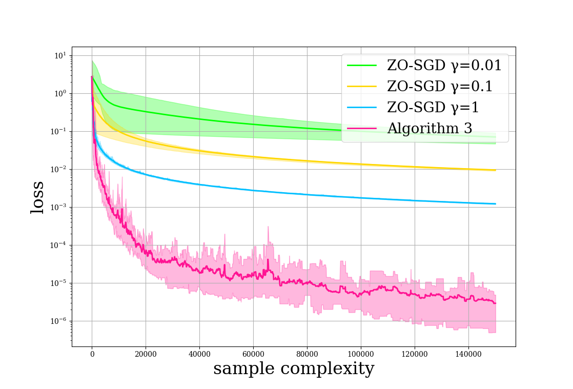
Figure 2: Training losses versus sample complexity for Algorithm 3 and ZO-SGD. The $x$-axis indicates number of function evaluations used. The solid lines are averaged over 10 runs. The shaded area above and below the solid lines shows the range (the maximum and minimum) of the 10 runs. For this experiment, “Iris Versicolour” and “Iris Virginica” are combined into a single class.

6 Conclusion

This paper investigates the stochastic optimization problem, particularly emphasizing the common scenario where the Hessian of the objective function over a data batch is low-rank. We introduce a stochastic zeroth-order cubic Newton method that demonstrates enhanced sample complexity compared to previous state-of-the-art approaches. This improvement is made possible through a novel Hessian estimation technique that capitalizes on the benefits of matrix completion while mitigating its limitations. The effectiveness of our method is supported by numerical studies.

Appendix A Omitted Proofs

A.1 Proof of Proposition 2

In this section, we provide a proof of Proposition 2, for which we first need the following fact.

Proposition 4.

For any integers $q>p\geq 0$. Define

$$J_{p,q}:=\int_{0}^{\pi}\cos^{p}x\sin^{q}x\,\mathrm{d}x.$$

It holds that

• $J_{0,q}=\frac{\sqrt{\pi}\Gamma(\frac{q+1}{2})}{\Gamma(\frac{q+2}{2})}$,

• $J_{p,q}=\frac{p-1}{p+q}J_{p-2,q}$ for all $p\geq 2$

Proof.

For the recursive formula, note that

$$J_{p,q}= \;\int_{0}^{\pi}\cos^{p}x\sin^{q}x\,\mathrm{d}x=\int_{0}^{\pi}\cos^{p-1}x\sin^{q}x\,\mathrm{d}\sin x$$

$$= \;\cos^{p-1}x\sin^{q+1}x\big{|}_{0}^{\pi}-(p-1)\int_{0}^{\pi}\sin x\cos^{p-2}x(-\sin x)\sin^{q}x\mathrm{d}x$$

$$-q\int_{0}^{\pi}\sin x\cos^{p-1}x\sin^{q-1}x\cos x\mathrm{d}x$$

$$= \;(p-1)J_{p-2,q+2}-qJ_{p,q}=(p-1)\left(J_{p-2,q}-J_{p,q}\right)-qJ_{p,q},$$

which gives $J_{p,q}=\frac{p-1}{p+q}J_{p-2,q}.$

∎

Proof of Proposition 2.

$$\mathbb{E}\left[v_{1}^{p}v_{2}^{2}\right]=\frac{1}{A_{n-1}}\int_{0}^{2\pi}\int_{0}^{\pi}\cdots\int_{0}^{\pi}\int_{0}^{\pi} \cos^{p}(\phi_{1})\sin^{2}(\phi_{1})\cos^{2}(\phi_{2})\sin^{n-2}(\phi_{1})$$

$$\cdots\sin(\phi_{n-2})\mathrm{d}\phi_{1}\mathrm{d}\phi_{2}\cdots\mathrm{d}\phi_{n-2}\mathrm{d}\phi_{n-1},$$

where $A_{n-1}$ is the area of the unit sphere:

$$A_{n-1}:=\int_{0}^{2\pi}\int_{0}^{\pi}\cdots\int_{0}^{\pi}\int_{0}^{\pi}\sin^{n-2}(\phi_{1})\cdots\sin(\phi_{n-2})\mathrm{d}\phi_{1}\mathrm{d}\phi_{2}\cdots\mathrm{d}\phi_{n-2}\mathrm{d}\phi_{n-1}.$$

Therefore, we have

$$\mathbb{E}\left[v_{1}^{p}v_{2}^{2}\right]= \;\frac{\int_{0}^{\pi}\int_{0}^{\pi}\cos^{p}(\phi_{1})\sin^{n}(\phi_{1})\cos^{2}(\phi_{2})\sin^{n-3}(\phi_{2})\mathrm{d}\phi_{1}\mathrm{d}\phi_{2}}{\int_{0}^{\pi}\int_{0}^{\pi}\sin^{n-2}(\phi_{1})\sin^{n-3}(\phi_{2})\mathrm{d}\phi_{1}\mathrm{d}\phi_{2}}$$

$$= \;\frac{\left(\frac{(p-1)(p-3)\cdots 1}{(n+p)(n+p-2)\cdots(n+2)}\right)\sqrt{\pi}\frac{\Gamma(\frac{n+1}{2})}{\Gamma(\frac{n+2}{2})}\frac{1}{n-1}\sqrt{\pi}\frac{\Gamma(\frac{n-2}{2})}{\Gamma(\frac{n-1}{2})}}{\pi\frac{\Gamma(\frac{n-1}{2})}{\Gamma(\frac{n}{2})}\cdot\frac{\Gamma(\frac{n-2}{2})}{\Gamma(\frac{n-1}{2})}},$$

where the last line uses Proposition 4. By simplifying terms in the above equation, we get

$$\mathbb{E}\left[v_{1}^{p}v_{2}^{2}\right]=\frac{(p-1)(p-3)\cdots 1}{(n+p)(n+p-2)\cdots(n+2)}\cdot\frac{1}{n-1}\cdot\frac{n-1}{n}=\frac{(p-1)(p-3)\cdots 1}{(n+p)(n+p-2)\cdots(n+2)}\cdot\frac{1}{n}.$$

Therefore, for $i\neq j$, we have

$$\mathbb{E}\left[u_{i}^{2p}v_{i}^{2p}v_{j}^{2}\right]\leq\frac{(2p-1)(2p-3)\cdots 1}{n(n+2)\cdots(n+2p-2)}\cdot\frac{(2p-1)(2p-3)\cdots 1}{(n+2p)(n+2p-2)\cdots(n+2)}\cdot\frac{1}{n}\leq\frac{(2p)!}{n^{2p+1}}.$$

∎

A.2 Proof of Lemma 9

Proof of Lemma 9.

When $H\succeq 0$, the statement is true. If $H\not\succeq 0$, without loss of generality, we assume that $H=\operatorname{diag}(\lambda_{1},\lambda_{2},\cdots,\lambda_{n})$ and $\lambda_{1}\geq\lambda_{2}\geq\cdots\geq\lambda_{m}>\lambda_{m+1}=\cdots=\lambda_{n}$. Let $v_{u}(\mathbf{z}):=\left<\mathbf{g},\mathbf{z}\right>+\frac{1}{2}\left<H\mathbf{z},\mathbf{z}\right>+\frac{M}{6}\|\mathbf{z}\|^{3},\mathbf{z}\in\mathbb{R}^{n}$ and $v_{l}(r):=-\frac{1}{2}\left<(H+\frac{Mr}{2}I)^{-1}\mathbf{g},\mathbf{g}\right>-\frac{M}{12}r^{3},r>-\frac{2\lambda_{n}}{M}$. We first show that

$$\min_{\mathbf{z}}v_{u}(\mathbf{z})\geq\sup_{r>-\frac{2\lambda_{n}}{M}}v_{l}(r).$$ (50)

Indeed,

$$\min_{\mathbf{z}}v_{u}(\mathbf{z}) =\min_{\mathbf{z},\tau\geq 0,\|\mathbf{z}\|^{2}\leq\tau}\left<\mathbf{g},\mathbf{z}\right>+\frac{1}{2}\left<H\mathbf{z},\mathbf{z}\right>+\frac{M}{6}\|\tau\|^{\frac{3}{2}}$$

$$=\min_{\mathbf{z},\tau\geq 0}\sup_{r\geq 0}\left<\mathbf{g},\mathbf{z}\right>+\frac{1}{2}\left<H\mathbf{z},\mathbf{z}\right>+\frac{M}{6}\|\tau\|^{\frac{3}{2}}+\frac{M}{4}r(\|\mathbf{z}\|^{2}-\tau)$$

$$\geq\sup_{r\geq 0}\min_{\mathbf{z},\tau\geq 0}\left<\mathbf{g},\mathbf{z}\right>+\frac{1}{2}\left<H\mathbf{z},\mathbf{z}\right>+\frac{M}{6}\|\tau\|^{\frac{3}{2}}+\frac{M}{4}r(\|\mathbf{z}\|^{2}-\tau)$$

$$=\sup_{r\geq 0}\min_{\mathbf{z}}\left<\mathbf{g},\mathbf{z}\right>+\frac{1}{2}\left<(H+\frac{M}{2}rI)\mathbf{z},\mathbf{z}\right>-\frac{M}{12}r^{3}$$

$$=\sup_{r>-\frac{2\lambda_{n}}{M}}\min_{\mathbf{z}}\left<\mathbf{g},\mathbf{z}\right>+\frac{1}{2}\left<(H+\frac{M}{2}rI)\mathbf{z},\mathbf{z}\right>-\frac{M}{12}r^{3}=\sup_{r>-\frac{2\lambda_{n}}{M}}v_{l}(r).$$

For $r>-\frac{2\lambda_{n}}{M}$, $v_{l}(r)$ is differentiable at any $r>-\frac{2\lambda_{n}}{M}$ and $v^{\prime}_{l}(r)=\frac{M}{4}(\|\mathbf{z}(r)\|^{2}-r^{2})$ where $\mathbf{z}(r):=-(H+\frac{Mr}{2}I)^{-1}\mathbf{g}$. In addition,

$$v_{u}(\mathbf{z}(r))-v_{l}(r)=\frac{M}{12}\left(r+2\|\mathbf{z}(r)\|\right)\left(\|\mathbf{z}(r)\|-r\right)^{2}=\frac{4}{3M}\cdot\frac{r+2\|\mathbf{z}(r)\|}{\left(r+\|\mathbf{z}(r)\|\right)^{2}}\cdot\left(v_{l}^{\prime}(r)\right)^{2},$$ (51)

By (50) and (51), if $\sup_{r>-\frac{2\lambda_{n}}{M}}v_{l}(r)$ is attained at some $r^{*}>-\frac{2\lambda_{n}}{M}$, then $v_{l}^{\prime}(r^{*})=0$. This implies that $\min_{\mathbf{z}}v_{u}(\mathbf{z})=\sup_{r>-\frac{2\lambda_{n}}{M}}v_{l}(r)$ and $\|\mathbf{z}^{*}\|=\|\mathbf{z}(r^{*})\|=r^{*}>-\frac{2\lambda_{n}}{M}$. Therefore $H+\frac{1}{2}M\|\mathbf{z}^{*}\|I\succeq 0$.

Otherwise $g_{m+1}=\cdots=g_{n}=0$. And we consider $\mathbf{g}_{\delta}:=\mathbf{g}+\delta\mathbf{e}_{n}$ where $\delta>0$ and $\mathbf{e}_{n}=(0,\cdots,0,1)^{\top}$. Let $v_{u,\delta}(\mathbf{z}):=v_{u}(\mathbf{z})+\delta z_{n}=\left<\mathbf{g}_{\delta},\mathbf{z}\right>+\frac{1}{2}\left<H\mathbf{z},\mathbf{z}\right>+\frac{M}{6}\|\mathbf{z}\|^{3}$ and $v_{l,\delta}(r):=-\frac{1}{2}\left<(H+\frac{Mr}{2}I)^{-1}\mathbf{g}_{\delta},\mathbf{g}_{\delta}\right>-\frac{M}{12}r^{3}$. Then $\lim_{r\to-\lambda_{n}}v^{\prime}_{l,\delta}(r)=+\infty$, $\lim_{r\to\infty}v^{\prime}_{l,\delta}(r)=-\infty$ and by continuity $\sup_{r>-\frac{2\lambda_{n}}{M}}v_{l,\delta}(r)$ is achieved by some $r_{\delta}^{*}>-\frac{2\lambda_{n}}{M}$. As a consequence, the minimizer of $v_{u,\delta}(\mathbf{z})$ is $\mathbf{z}_{\delta}^{*}=(H+\frac{M}{2}r_{\delta}^{*}I)^{-1}\mathbf{g}_{\delta}$ and $\|\mathbf{z}_{\delta}^{*}\|=r_{\delta}^{*}$. Consider $\delta_{k}=\frac{1}{k}$, then $\{v_{u,\delta_{k}}\}_{k=1}^{\infty}$ is equi-coercive in $\mathbb{R}^{n}$ and $\Gamma$-converge to $v_{u}$, $\{v_{l,\delta_{k}}\}_{k=1}^{\infty}$ is equi-coercive in $\{r:r>-\frac{2\lambda_{n}}{M}\}$ and $\Gamma$-converge to $v_{l}$. By fundamental theorem of $\Gamma$-convergence, $\mathbf{z}_{0}^{*}:=\lim_{k\to\infty}\mathbf{z}_{\delta_{k}}^{*}$ is the optimizer of $v_{u}$ and $\lim_{k\to\infty}r_{\delta_{k}}^{*}$ is the optimizer of $v_{l}$. By continuity of norm and since $-\frac{2\lambda_{n}}{M}$ is the unique minimizer of $v_{l}$, we have $\|\mathbf{z}_{0}^{*}\|=\lim_{k\to\infty}r_{\delta_{k}}^{*}=-\frac{2\lambda_{n}}{M}$ and therefore $H+\frac{1}{2}M\|\mathbf{z}^{*}\|I\succeq 0$.

∎

A.3 Additional Detail for Lemma 4

In this part, we provide details for bounding the moments of $Z$, where $Z$ is defined in (22).

Derivation of Eq. 26.

The second moment of $Z$ satisfies

$$\mathbb{E}\left[Z^{2}\right]= \;n^{4}\mathbb{E}\left[\left(\mathbf{u}_{r+1:}\mathbf{u}_{:r}^{\top}\otimes\mathbf{v}_{:r}\mathbf{v}^{\top}+\mathbf{u}_{:r}\mathbf{u}_{r+1:}^{\top}\otimes\mathbf{v}\mathbf{v}_{:r}^{\top}\right)^{2}\right]$$

$$= \;n^{4}\mathbb{E}\left[\left(\mathbf{u}_{r+1:}\mathbf{u}_{:r}^{\top}\mathbf{u}_{:r}\mathbf{u}_{r+1:}^{\top}\right)\otimes\left(\mathbf{v}_{:r}\mathbf{v}_{:r}^{\top}\right)+\left(\mathbf{u}_{:r}\mathbf{u}_{r+1:}^{\top}\mathbf{u}_{r+1:}\mathbf{u}_{:r}^{\top}\otimes\mathbf{v}\mathbf{v}_{:r}^{\top}\mathbf{v}_{:r}\mathbf{v}^{\top}\right)\right]$$

$$\preceq \;\frac{n^{2}r}{(n+2)}I_{n^{2}}+3nrI_{n^{2}}\preceq 4nrI_{n^{2}},$$ (52)

where the last line uses Proposition 2.

The $2p$-th power of $Z$ is

$$Z^{2p}= \;n^{4p}\left(\mathbf{u}_{r+1:}\mathbf{u}_{:r}^{\top}\mathbf{u}_{:r}\mathbf{u}_{r+1:}^{\top}\right)^{p}\otimes\left(\mathbf{v}_{:r}\mathbf{v}_{:r}^{\top}\right)^{p}$$

$$+n^{4p}\left(\mathbf{u}_{:r}\mathbf{u}_{r+1:}^{\top}\mathbf{u}_{r+1:}\mathbf{u}_{:r}^{\top}\right)^{p}\otimes\left(\mathbf{v}\mathbf{v}_{:r}^{\top}\mathbf{v}_{:r}\mathbf{v}^{\top}\right)^{p}$$

$$\preceq \;n^{4p}\left(\mathbf{u}_{:r}^{\top}\mathbf{u}_{:r}\right)^{p}\mathbf{u}_{r+1:}\mathbf{u}_{r+1:}^{\top}\otimes\left(\mathbf{v}_{:r}^{\top}\mathbf{v}_{:r}\right)^{p-1}\mathbf{v}_{:r}\mathbf{v}_{:r}^{\top}$$

$$+n^{4p}\left(\mathbf{u}_{:r}^{\top}\mathbf{u}_{:r}\right)^{p-1}\mathbf{u}_{:r}\mathbf{u}_{:r}^{\top}\otimes\left(\mathbf{v}_{:r}^{\top}\mathbf{v}_{:r}\right)^{p}\mathbf{v}\mathbf{v}^{\top}$$

and the $(2p+1)$-th power of $Z$ is

$$Z^{2p+1}= \;n^{4p+2}\left(\mathbf{u}_{r+1:}\mathbf{u}_{:r}^{\top}\mathbf{u}_{:r}\mathbf{u}_{r+1:}^{\top}\right)^{p}\mathbf{u}_{r+1:}\mathbf{u}_{:r}^{\top}\otimes\left(\mathbf{v}_{:r}\mathbf{v}_{:r}^{\top}\right)^{p}\mathbf{v}_{:r}\mathbf{v}^{\top}$$

$$+\left(\mathbf{u}_{:r}\mathbf{u}_{r+1:}^{\top}\mathbf{u}_{r+1:}\mathbf{u}_{:r}^{\top}\right)^{p}\mathbf{u}_{:r}\mathbf{u}_{r+1:}^{\top}\otimes\left(\mathbf{v}\mathbf{v}_{:r}^{\top}\mathbf{v}_{:r}\mathbf{v}^{\top}\right)^{p}\mathbf{v}\mathbf{v}_{:r}^{\top}.$$

Thus by Proposition 2, we have, for $p=2,3,4,\cdots$

$$\mathbb{E}\left[Z^{2p}\right]\preceq \;n^{4p}\mathbb{E}\left[r^{p-1}\left(\sum_{i=1}^{r}u_{i}^{2p}\right)\mathbf{u}_{r+1:}\mathbf{u}_{r+1:}^{\top}\otimes r^{p-2}\left(\sum_{i=1}^{r}v_{i}^{2p-2}\right)\mathbf{v}\mathbf{v}^{\top}\right]$$

$$+n^{4p}\mathbb{E}\left[r^{p-2}\left(\sum_{i=1}^{r}u_{i}^{2p-2}\right)\mathbf{u}_{:r}\mathbf{u}_{:r}^{\top}\otimes r^{p-1}\left(\sum_{i=1}^{r}v_{i}^{2p}\right)\mathbf{v}\mathbf{v}^{\top}\right]$$

$$\preceq \;2n^{4p}r^{2p-1}\cdot\frac{(2p+1)(2p-1)\cdots 1}{n(n+2)\cdots(n+2p)}\cdot\frac{(2p-1)(2p-3)\cdots 1}{n(n+2)\cdots(n+2p-2)}I_{n^{2}}$$

$$\preceq \;\frac{(2p)!}{2}(8nr)^{2p-1}I_{n^{2}}.$$ (53)

For $Z^{2p+1}$ ($p\in\mathbb{N}$), we notice that

$$\mathbb{E}\left[\left(\mathbf{u}_{r+1:}\mathbf{u}_{:r}^{\top}\mathbf{u}_{:r}\mathbf{u}_{r+1:}^{\top}\right)^{p}\mathbf{u}_{r+1:}\mathbf{u}_{:r}^{\top}\right]=\mathbb{E}\left[\left(\mathbf{u}_{:r}\mathbf{u}_{r+1:}^{\top}\mathbf{u}_{r+1:}\mathbf{u}_{:r}^{\top}\right)^{p}\mathbf{u}_{:r}\mathbf{u}_{r+1:}^{\top}\right]=0,$$

since these terms only involve odd powers of the entries of $\mathbf{u}$. Therefore

$$\mathbb{E}\left[Z^{2p+1}\right]=0,\quad\text{ for }p=0,1,2,\cdots$$ (54)

Collecting terms from (52), (53) and (54) gives (26)∎

Appendix B Additional Experiments

In this section, we repeat the experiments in Section 5.1, with different choice of the matrix size $n$. The results are in Tables 4-6.

Number of measurements $M$	Error in Frobenius norm $\|H-\widehat{H}\|_{F}$	Relative error: $\|H-\widehat{H}\|_{F}/\|H\|_{F}$
$nr$	41.69 $\pm$ 5.48	0.46 $\pm$ 4.25e-2
$2nr$	3.58e-4 $\pm$ 2.60e-4	3.48e-6 $\pm$ 2.26e-6
$3nr$	1.49e-5 $\pm$ 7.57e-6	1.58e-7 $\pm$ 8.45e-8

Table 4: Error (in Frobenius norm) and relative errors under different numbers of measurements. In this experiment, we use $n=40$ and $r=5$. Each cell on the second/third column summarizes the recovery error for ten recovery runs, each with a randomly generated low-rank matrix $H$. The results are listed in a “mean $\pm$ std” format.

Number of measurements $M$	Error in Frobenius norm $\|H-\widehat{H}\|_{F}$	Relative error: $\|H-\widehat{H}\|_{F}/\|H\|_{F}$
$nr$	83.72 $\pm$ 8.72	0.59 $\pm$ 4.24e-2
$2nr$	1.62e-3 $\pm$ 7.92e-4	1.14e-5 $\pm$ 5.37e-6
$3nr$	3.52e-4 $\pm$ 2.52e-4	2.40e-6 $\pm$ 1.37e-6

Table 5: Error (in Frobenius norm) and relative errors under different numbers of measurements. In this experiment, we use $n=60$ and $r=5$. Each cell on the second/third column summarizes the recovery error for ten recovery runs, each with a randomly generated low-rank matrix $H$. The results are listed in a “mean $\pm$ std” format.

Number of measurements $M$	Error in Frobenius norm $\|H-\widehat{H}\|_{F}$	Relative error: $\|H-\widehat{H}\|_{F}/\|H\|_{F}$
$nr$	111.70 $\pm$ 14.38	0.62 $\pm$ 5.49e-2
$2nr$	1.78e-2 $\pm$ 8.63e-3	9.39e-5 $\pm$ 4.19e-5
$3nr$	1.42e-3 $\pm$ 1.02e-3	7.85e-6 $\pm$ 5.61e-6

Table 6: Error (in Frobenius norm) and relative errors under different numbers of measurements. In this experiment, we use $n=80$ and $r=5$. Each cell on the second/third column summarizes the recovery error for ten recovery runs, each with a randomly generated low-rank matrix $H$. The results are listed in a “mean $\pm$ std” format.

Appendix C Table of Notations

Table 7: List of notations.

Notation	Explanation
$n$	dimension of the stochastic optimization problem
$r$	upper bound of the rank of Hessian
$F(\mathbf{x})$	the objective function
$F^{*}$	the minimum of $F$
$\xi$	index for a (batch of) training data
$f(\mathbf{x};\xi)$	function evaluation corresponding to $\xi$
$\mathcal{P}_{i}$	matrix measurement operation
$\mathcal{S}$	the sampler constructed with $\mathcal{P}_{i}$
$T$	the total time horizon
$m_{1}$	the number of function evaluations used for gradient
$m_{2}$	the number of function evaluations used for Hessian
$\mathbf{u}_{i},\mathbf{v}_{i}$	measurement vectors uniformly distributed over the unit sphere
$L_{1}$	gradient Lipschitz constant
$L_{2}$	Hessian Lipschitz constant
$\delta$	finite-difference granularity
$M$	the number of measurements
$H$	a random symmetric matrix determined by $\{\mathbf{u}_{i},\mathbf{v}_{i}\}_{i}$
$H_{r}$	the best rank-$r$ approximation of the real Hessian
$\widehat{H}$	the solution of the convex program (5)
$\mathbf{g}_{t}$	the gradient estimator at time $t$
$\widehat{H}_{t}$	the Hessian estimator at time $t$
$\alpha$	regularizer for Newton step
$\epsilon$	the gap between $H_{r}$ and the real Hessian
$\beta,\eta,\kappa$	arbitrarily small quantity
$\mathcal{A}$	a subspace of $\mathbb{R}^{n\times n}$ (Eq. 12)
$\mathcal{P}_{\mathcal{A}}$	a projection operation onto $\mathcal{A}$
$\sigma_{1},\sigma_{2},\tau_{2}$	the upper bound of some central moments

References

- Ahn et al., (2023) Ahn, J., Elmahdy, A., Mohajer, S., and Suh, C. (2023). On the fundamental limits of matrix completion: Leveraging hierarchical similarity graphs. IEEE Transactions on Information Theory, pages 1–1.
- Balasubramanian and Ghadimi, (2021) Balasubramanian, K. and Ghadimi, S. (2021). Zeroth-order nonconvex stochastic optimization: Handling constraints, high dimensionality, and saddle points. Foundations of Computational Mathematics, pages 1–42.
- Balasubramanian and Ghadimi, (2022) Balasubramanian, K. and Ghadimi, S. (2022). Zeroth-order nonconvex stochastic optimization: Handling constraints, high dimensionality, and saddle points. Foundations of Computational Mathematics, 22(1):35–76.
- Bandeira et al., (2012) Bandeira, A. S., Scheinberg, K., and Vicente, L. N. (2012). Computation of sparse low degree interpolating polynomials and their application to derivative-free optimization. Mathematical Programming, 134(1):223–257.
- Bhatia, (1997) Bhatia, R. (1997). Matrix analysis. Graduate Texts in Mathematics.
- Broyden et al., (1973) Broyden, C. G., Dennis Jr, J. E., and Moré, J. J. (1973). On the local and superlinear convergence of quasi-newton methods. IMA Journal of Applied Mathematics, 12(3):223–245.
- (7) Cai, H., McKenzie, D., Yin, W., and Zhang, Z. (2022a). A one-bit, comparison-based gradient estimator. Applied and Computational Harmonic Analysis, 60:242–266.
- (8) Cai, H., Mckenzie, D., Yin, W., and Zhang, Z. (2022b). Zeroth-order regularized optimization (zoro): Approximately sparse gradients and adaptive sampling. SIAM Journal on Optimization, 32(2):687–714.
- Cai et al., (2010) Cai, J.-F., Candès, E. J., and Shen, Z. (2010). A singular value thresholding algorithm for matrix completion. SIAM Journal on optimization, 20(4):1956–1982.
- Candes and Recht, (2012) Candes, E. and Recht, B. (2012). Exact matrix completion via convex optimization. Communications of the ACM, 55(6):111–119.
- Candes and Plan, (2010) Candes, E. J. and Plan, Y. (2010). Matrix completion with noise. Proceedings of the IEEE, 98(6):925–936.
- Candès and Tao, (2010) Candès, E. J. and Tao, T. (2010). The power of convex relaxation: Near-optimal matrix completion. IEEE Transactions on Information Theory, 56(5):2053–2080.
- Chandrasekaran et al., (2012) Chandrasekaran, V., Recht, B., Parrilo, P. A., and Willsky, A. S. (2012). The convex geometry of linear inverse problems. Foundations of Computational Mathematics, 12(6):805–849.
- Chen et al., (2017) Chen, P.-Y., Zhang, H., Sharma, Y., Yi, J., and Hsieh, C.-J. (2017). Zoo: Zeroth order optimization based black-box attacks to deep neural networks without training substitute models. In Proceedings of the 10th ACM workshop on artificial intelligence and security, pages 15–26.
- Chen et al., (2019) Chen, X., Liu, S., Xu, K., Li, X., Lin, X., Hong, M., and Cox, D. (2019). Zo-adamm: Zeroth-order adaptive momentum method for black-box optimization. Advances in neural information processing systems, 32.
- Chen, (2015) Chen, Y. (2015). Incoherence-optimal matrix completion. IEEE Transactions on Information Theory, 61(5):2909–2923.
- Chen et al., (2020) Chen, Y., Chi, Y., Fan, J., Ma, C., and Yan, Y. (2020). Noisy matrix completion: Understanding statistical guarantees for convex relaxation via nonconvex optimization. SIAM journal on optimization, 30(4):3098–3121.
- (18) Conn, A. R., Scheinberg, K., and Vicente, L. N. (2008a). Geometry of interpolation sets in derivative free optimization. Mathematical Programming, 111(1):141–172.
- (19) Conn, A. R., Scheinberg, K., and Vicente, L. N. (2008b). Geometry of sample sets in derivative-free optimization: polynomial regression and underdetermined interpolation. IMA Journal of Numerical Analysis, 28(4):721–748.
- Conn et al., (2009) Conn, A. R., Scheinberg, K., and Vicente, L. N. (2009). Introduction to derivative-free optimization. SIAM.
- Davidon, (1991) Davidon, W. C. (1991). Variable metric method for minimization. SIAM Journal on optimization, 1(1):1–17.
- Diamond and Boyd, (2016) Diamond, S. and Boyd, S. (2016). CVXPY: A Python-embedded modeling language for convex optimization. Journal of Machine Learning Research, 17(83):1–5.
- Duchi et al., (2015) Duchi, J. C., Jordan, M. I., Wainwright, M. J., and Wibisono, A. (2015). Optimal rates for zero-order convex optimization: The power of two function evaluations. IEEE Transactions on Information Theory, 61(5):2788–2806.
- El Mestari et al., (2024) El Mestari, S. Z., Lenzini, G., and Demirci, H. (2024). Preserving data privacy in machine learning systems. Computers & Security, 137:103605.
- Eldar et al., (2012) Eldar, Y., Needell, D., and Plan, Y. (2012). Uniqueness conditions for low-rank matrix recovery. Applied and Computational Harmonic Analysis, 33(2):309–314.
- Fan et al., (2021) Fan, J., Wang, W., and Zhu, Z. (2021). A shrinkage principle for heavy-tailed data: High-dimensional robust low-rank matrix recovery. The Annals of Statistics, 49(3):1239 – 1266.
- Fazel, (2002) Fazel, M. (2002). Matrix rank minimization with applications. PhD thesis, PhD thesis, Stanford University.
- Feng and Wang, (2023) Feng, Y. and Wang, T. (2023). Stochastic zeroth-order gradient and Hessian estimators: variance reduction and refined bias bounds. Information and Inference: A Journal of the IMA, 12(3):1514–1545.
- Fisher, (1936) Fisher, R. A. (1936). Iris. UCI Machine Learning Repository. DOI: https://doi.org/10.24432/C56C76.
- Flaxman et al., (2005) Flaxman, A. D., Kalai, A. T., and McMahan, H. B. (2005). Online convex optimization in the bandit setting: gradient descent without a gradient. In Proceedings of the sixteenth annual ACM-SIAM symposium on Discrete algorithms, pages 385–394.
- Fletcher, (2000) Fletcher, R. (2000). Practical methods of optimization. John Wiley & Sons.
- Fornasier et al., (2011) Fornasier, M., Rauhut, H., and Ward, R. (2011). Low-rank matrix recovery via iteratively reweighted least squares minimization. SIAM Journal on Optimization, 21(4):1614–1640.
- Ghadimi and Lan, (2013) Ghadimi, S. and Lan, G. (2013). Stochastic first-and zeroth-order methods for nonconvex stochastic programming. SIAM journal on optimization, 23(4):2341–2368.
- Goldfarb, (1970) Goldfarb, D. (1970). A family of variable-metric methods derived by variational means. Mathematics of computation, 24(109):23–26.
- Gotoh et al., (2018) Gotoh, J.-y., Takeda, A., and Tono, K. (2018). Dc formulations and algorithms for sparse optimization problems. Mathematical Programming, 169(1):141–176.
- Gross, (2011) Gross, D. (2011). Recovering low-rank matrices from few coefficients in any basis. IEEE Transactions on Information Theory, 57(3):1548–1566.
- Hare et al., (2023) Hare, W., Jarry-Bolduc, G., and Planiden, C. (2023). A matrix algebra approach to approximate Hessians. IMA Journal of Numerical Analysis, 44(4):2220–2250.
- Hu et al., (2012) Hu, Y., Zhang, D., Ye, J., Li, X., and He, X. (2012). Fast and accurate matrix completion via truncated nuclear norm regularization. IEEE transactions on pattern analysis and machine intelligence, 35(9):2117–2130.
- Jarry-Bolduc and Planiden, (2023) Jarry-Bolduc, G. and Planiden, C. (2023). Using generalized simplex methods to approximate derivatives.
- Keshavan et al., (2010) Keshavan, R. H., Montanari, A., and Oh, S. (2010). Matrix completion from a few entries. IEEE Transactions on Information Theory, 56(6):2980–2998.
- Lee and Bresler, (2010) Lee, K. and Bresler, Y. (2010). Admira: Atomic decomposition for minimum rank approximation. IEEE Transactions on Information Theory, 56(9):4402–4416.
- Li et al., (2022) Li, J., Balasubramanian, K., and Ma, S. (2022). Stochastic zeroth-order riemannian derivative estimation and optimization. Mathematics of Operations Research.
- Li et al., (2023) Li, J., Balasubramanian, K., and Ma, S. (2023). Stochastic zeroth-order riemannian derivative estimation and optimization. Mathematics of Operations Research, 48(2):1183–1211.
- Lieb, (1973) Lieb, E. H. (1973). Convex trace functions and the wigner-yanase-dyson conjecture. Advances in Mathematics, 11(3):267–288.
- Liu et al., (2020) Liu, S., Chen, P.-Y., Kailkhura, B., Zhang, G., Hero III, A. O., and Varshney, P. K. (2020). A primer on zeroth-order optimization in signal processing and machine learning: Principals, recent advances, and applications. IEEE Signal Processing Magazine, 37(5):43–54.
- Liu et al., (2018) Liu, S., Kailkhura, B., Chen, P.-Y., Ting, P., Chang, S., and Amini, L. (2018). Zeroth-order stochastic variance reduction for nonconvex optimization. Advances in Neural Information Processing Systems, 31.
- Mohan and Fazel, (2012) Mohan, K. and Fazel, M. (2012). Iterative reweighted algorithms for matrix rank minimization. The Journal of Machine Learning Research, 13(1):3441–3473.
- Needell and Tropp, (2009) Needell, D. and Tropp, J. A. (2009). Cosamp: Iterative signal recovery from incomplete and inaccurate samples. Applied and computational harmonic analysis, 26(3):301–321.
- Negahban and Wainwright, (2012) Negahban, S. and Wainwright, M. J. (2012). Restricted strong convexity and weighted matrix completion: Optimal bounds with noise. The Journal of Machine Learning Research, 13(1):1665–1697.
- Nesterov, (2008) Nesterov, Y. (2008). Accelerating the cubic regularization of newton’s method on convex problems. Mathematical Programming, 112(1):159–181.
- Nesterov, (2018) Nesterov, Y. (2018). Lectures on convex optimization, volume 137. Springer.
- Nesterov and Polyak, (2006) Nesterov, Y. and Polyak, B. T. (2006). Cubic regularization of newton method and its global performance. Mathematical Programming, 108(1):177–205.
- Nesterov and Spokoiny, (2017) Nesterov, Y. and Spokoiny, V. (2017). Random gradient-free minimization of convex functions. Foundations of Computational Mathematics, 17(2):527–566.
- Recht, (2011) Recht, B. (2011). A simpler approach to matrix completion. Journal of Machine Learning Research, 12(12).
- Recht et al., (2010) Recht, B., Fazel, M., and Parrilo, P. A. (2010). Guaranteed minimum-rank solutions of linear matrix equations via nuclear norm minimization. SIAM Review, 52(3):471–501.
- Ren-Pu and Powell, (1983) Ren-Pu, G. and Powell, M. J. (1983). The convergence of variable metric matrices in unconstrained optimization. Mathematical programming, 27:123–143.
- Rios and Sahinidis, (2013) Rios, L. M. and Sahinidis, N. V. (2013). Derivative-free optimization: a review of algorithms and comparison of software implementations. Journal of Global Optimization, 56(3):1247–1293.
- Rodomanov and Nesterov, (2022) Rodomanov, A. and Nesterov, Y. (2022). Rates of superlinear convergence for classical quasi-newton methods. Mathematical Programming, 194(1):159–190.
- Rohde and Tsybakov, (2011) Rohde, A. and Tsybakov, A. B. (2011). Estimation of high-dimensional low-rank matrices. The Annals of Statistics, 39(2):887 – 930.
- Rong et al., (2021) Rong, Y., Wang, Y., and Xu, Z. (2021). Almost everywhere injectivity conditions for the matrix recovery problem. Applied and Computational Harmonic Analysis, 50:386–400.
- Shahriari et al., (2015) Shahriari, B., Swersky, K., Wang, Z., Adams, R. P., and De Freitas, N. (2015). Taking the human out of the loop: A review of bayesian optimization. Proceedings of the IEEE, 104(1):148–175.
- Shanno, (1970) Shanno, D. F. (1970). Conditioning of quasi-newton methods for function minimization. Mathematics of computation, 24(111):647–656.
- Spall, (2000) Spall, J. C. (2000). Adaptive stochastic approximation by the simultaneous perturbation method. IEEE transactions on automatic control, 45(10):1839–1853.
- Stein, (1981) Stein, C. M. (1981). Estimation of the Mean of a Multivariate Normal Distribution. The Annals of Statistics, 9(6):1135 – 1151.
- Tan et al., (2011) Tan, V. Y., Balzano, L., and Draper, S. C. (2011). Rank minimization over finite fields: Fundamental limits and coding-theoretic interpretations. IEEE transactions on information theory, 58(4):2018–2039.
- Tanner and Wei, (2016) Tanner, J. and Wei, K. (2016). Low rank matrix completion by alternating steepest descent methods. Applied and Computational Harmonic Analysis, 40(2):417–429.
- Taylor, (1715) Taylor, B. (1715). Methodus Incrementorum Directa et Inversa. London: William Innys.
- Tripuraneni et al., (2018) Tripuraneni, N., Stern, M., Jin, C., Regier, J., and Jordan, M. I. (2018). Stochastic cubic regularization for fast nonconvex optimization. In Bengio, S., Wallach, H., Larochelle, H., Grauman, K., Cesa-Bianchi, N., and Garnett, R., editors, Advances in Neural Information Processing Systems, volume 31. Curran Associates, Inc.
- Tropp, (2012) Tropp, J. A. (2012). User-friendly tail bounds for sums of random matrices. Foundations of computational mathematics, 12:389–434.
- Tropp et al., (2015) Tropp, J. A. et al. (2015). An introduction to matrix concentration inequalities. Foundations and Trends® in Machine Learning, 8(1-2):1–230.
- Tu et al., (2019) Tu, C.-C., Ting, P., Chen, P.-Y., Liu, S., Zhang, H., Yi, J., Hsieh, C.-J., and Cheng, S.-M. (2019). Autozoom: Autoencoder-based zeroth order optimization method for attacking black-box neural networks. In Proceedings of the AAAI conference on artificial intelligence, volume 33, pages 742–749.
- Vandereycken, (2013) Vandereycken, B. (2013). Low-rank matrix completion by riemannian optimization. SIAM Journal on Optimization, 23(2):1214–1236.
- Wang, (2023) Wang, T. (2023). On sharp stochastic zeroth-order Hessian estimators over Riemannian manifolds. Information and Inference: A Journal of the IMA, 12(2):787–813.
- Wang et al., (2018) Wang, Y., Du, S., Balakrishnan, S., and Singh, A. (2018). Stochastic zeroth-order optimization in high dimensions. In International Conference on Artificial Intelligence and Statistics, pages 1356–1365. PMLR.
- Wang et al., (2014) Wang, Z., Lai, M.-J., Lu, Z., Fan, W., Davulcu, H., and Ye, J. (2014). Rank-one matrix pursuit for matrix completion. In Xing, E. P. and Jebara, T., editors, Proceedings of the 31st International Conference on Machine Learning, volume 32 of Proceedings of Machine Learning Research, pages 91–99, Bejing, China. PMLR.
- Wen et al., (2012) Wen, Z., Yin, W., and Zhang, Y. (2012). Solving a low-rank factorization model for matrix completion by a nonlinear successive over-relaxation algorithm. Mathematical Programming Computation, 4(4):333–361.
- Xiaojun Mao and Wong, (2019) Xiaojun Mao, S. X. C. and Wong, R. K. W. (2019). Matrix completion with covariate information. Journal of the American Statistical Association, 114(525):198–210.
- Xu and Zhang, (2001) Xu, C. and Zhang, J. (2001). A survey of quasi-newton equations and quasi-newton methods for optimization. Annals of Operations research, 103:213–234.
- Zhang et al., (2014) Zhang, L., Mahdavi, M., Jin, R., Yang, T., and Zhu, S. (2014). Random projections for classification: A recovery approach. IEEE Transactions on Information Theory, 60(11):7300–7316.
- Zhu, (2012) Zhu, S. (2012). A short note on the tail bound of wishart distribution. arXiv preprint arXiv:1212.5860.