The $s$-Energy and Its Applications

Abstract

Averaging dynamics drives countless processes in physics, biology, engineering, and the social sciences. In recent years, the $s$-energy has emerged as a useful tool for bounding the convergence rates of time-varying averaging systems. We derive new bounds on the $s$-energy, which we use to resolve a number of open questions in the areas of bird flocking, opinion dynamics, and distributed motion coordination. We also use our results to provide a theoretical validation for the idea of the “Overton Window” as an attracting manifold of viable group opinions. Our new bounds on the $s$-energy highlight its dependency on the connectivity of the underlying networks. In this vein, we use the $s$-energy to explain the exponential gap in the convergence rates of stationary and time-varying consensus systems.

1 Introduction

Dynamics based on local averaging has been the object of considerable attention [7, 9, 10, 11, 12, 13, 29, 34, 35, 36, 37, 39, 40, 43, 44, 45, 46, 49, 51, 52, 55, 62]. The reason is the ubiquity of these systems, which are found in synchronization processes (e.g., fireflies, power grids, pacemaker cells, coupled oscillators), bird flocking, social epistemology, and opinion dynamics [9, 14, 16, 21, 23, 25, 63]. Agents interact across a time-varying network by averaging their state variables with those of their neighbors. Under mild conditions, such systems are known to converge to a fixed-point attractor.

Of course, the convergence rate of averaging dynamics depends on the underlying network sequences. The case of a single, fixed network is dual to a Markov chain and the convergence rate is given by the corresponding mixing time [41]. When networks are allowed to change over time, bounding the convergence rate becomes far more challenging and suitable analytical tools have been lacking. The introduction of the $s$-energy has given us access to the convergence rates of important instances of averaging dynamics [14]. In this work, we prove new bounds on the $s$-energy, which we then use to bound the convergence rates of systems for bird flocking, opinion dynamics, and distributed motion coordination. In particular, we prove that a group of birds with at most a constant number of flocks converges in polynonomial time; this is the first polynomial bound of its kind. We also provide a theoretical validation for the popular idea of the “Overton Window,” which we interpret as an attracting manifold of viable group opinions.

Our investigation highlights the key role played by network connectivity in the $s$-energy. It helps us resolve what has been a puzzling mystery for several years now: Previous work, indeed, has shown that convergence to equilibrium within $\varepsilon$ is reached in time at most $C\big{(}\log\frac{1}{\varepsilon}\big{)}^{n-1}$, where $n$ is the number of agents and $C$ is a parameter depending only on the networks’ characteristics [16, 29, 37, 55, 56]. When all of the communication networks are connected, however, the time bound drops to $C\log\frac{1}{\varepsilon}$. Such an exponential gap also appears in recent works on broadcast and consensus dynamics and hyper-torpid mixing [17, 20, 26, 27, 65]. We explain this gap by proving that the convergence time is actually of the form $C\big{(}\log\frac{1}{\varepsilon}\big{)}^{m}$, where $m<n$ is the maximum number of connected components at any time. This result follows from our new bounds on the $s$-energy.

Averaging dynamics.

Let $(G_{t})_{t\geq 0}$ be an infinite sequence of undirected graphs over the vertex set $[n]$. Each vertex has a self-loop. Let $P_{t}$ be the stochastic matrix of a weighted random walk over $G_{t}$. By construction, a matrix entry is positive if and only if it corresponds to an edge of $G_{t}$. Each row sums up to 1 and the diagonal is positive everywhere. We assume that the nonzero entries in $P_{t}$ are at least some fixed $\rho\in(0,1/2]$, called the weight threshold. Let $P_{\leq t}$ denote the product $P_{t}P_{t-1}\cdots P_{0}$. The set of orbits $(P_{\leq t}x)_{t\geq 0}$, over all $x\in\mathbb{R}^{n}$, defines an averaging system. It is sometimes called “consensus dynamics” in the literature [29]. In addition to the general case defined above, we also consider three special cases:

• rev:    a reversible averaging system assumes that all of the individual Markov chains $P_{t}$ are reversible and share the same stationary distribution. This means that $P_{t}=\text{diag}(q)^{-1}M_{t}$, where $M_{t}$ is symmetric with nonzero entries at least 1 and $q=M_{t}\mathbf{1}\preceq\mathbf{1}/\rho$. The stationary distribution is given by $q/\|q\|_{1}$.

• exp:    an expanding averaging system is a rev where $q=d\mathbf{1}$ and the connected components of each $G_{t}$ are $d$-regular expanders. Recall that a $d$-regular expander is a graph of degree $d$ such that, for any set $X$ of at most half of the vertices, we have $|\partial X|\geq h|X|$, where $\partial X$ is the set of edges with exactly one vertex in $X$; the factor $h$ is called the Cheeger constant.

• ran:  a random averaging system is a rev where $q=d\mathbf{1}$ with each $P_{t}$ is the simple random walk over a random $(d-1)$-regular graph $G_{t}$.

The $\bm{s}$-energy.

Given $x(0)\in\mathbb{R}^{n}$, we write $x(t+1)=P_{t}x(t)$ for $t\geq 0$, and refer to the $i$-th coordinate $x_{i}(t)$ as the position of agent $i$ at time $t$. The vector $x(t)$ provides an embedding of the graph $G_{t}$ over the reals. The union of the embedded edges of $G_{t}$ forms disjoint intervals, called blocks. Let $l_{1}(t),\ldots,l_{k_{t}}(t)$ be the lengths of these blocks and put $E_{s,t}=\sum_{i=1}^{k_{t}}l_{i}(t)^{s}$, with $s\in(0,1]$. For example, if, besides its self-loops, $G_{t}$ has four edges embedded as the intervals $[1,3]$, $[2,4]$, $[5,9]$, and $[6,9]$, then there are $k_{t}=2$ blocks $[1,4]$ and $[5,9]$; hence $E_{s,t}=3^{s}+4^{s}$ (Figure 1).

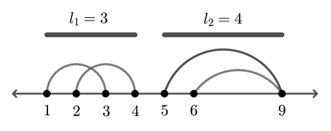
Figure 1: The graph $G_{t}$ is embedded on the real line (self-loops not shown) and $E_{s,t}=3^{s}+4^{s}$.

We define the $s$-energy $E_{s}=\sum_{t\geq 0}E_{s,t}$ and denote by $\mathcal{E}_{s}$ the supremum of $E_{s}\,$ over all $n$-vertex graph sequences $(G_{t})_{t\geq 0}$ and any initial position $x(0)\in[0,1]^{n}$. If we limit the sequences to include only graphs with at most $m$ connected components, then we denote the supremum by $\mathcal{E}_{m,s}$; note that $\mathcal{E}_{s}=\mathcal{E}_{n-1,s}$. The best known bound states that $\mathcal{E}_{s}\leq(3/\rho s)^{n-1}$ [16]. We prove the following results, all of which assume the same fixed weight threshold $\rho\in(0,1/2]$ and $s\in(0,1]$. The superscripts below indicate the type of averaging systems considered.

Theorem 1.1

  

1. $\mathcal{E}_{m,1}\leq 3en(1/\rho)^{\lfloor n/2\rfloor}$ and  $\mathcal{E}_{m,s}\leq(c/s)^{m}(1/\rho)^{n-1}$, where $c=O(mn)$.

2. $\mathcal{E}_{m,s}^{\text{\sc rev}}\leq(cn^{2}/\rho s)^{m}$, for constant $c>0$.

3. $\mathcal{E}_{1,s}^{\,\text{\sc exp}}=O(d^{3}/sh^{2})$  and  $\mathcal{E}_{m,s}^{\,\text{\sc exp}}\leq(c/s)^{m}$, where $c=O(d^{3}mn/h^{2})$.

4. $\mathbb{E}\,\mathcal{E}_{s}^{\,\text{\sc ran}}\leq c/s$, for constant $c>0$.

The bounds in (a) apply to any initial position $x(0)\in[0,1]^{n}$ or, equivalently, an initial diameter at most 1. For notational convenience, we use a slightly different assumption for the cases (b, c, d): we assume that the initial (scaled) variance $\sum_{i}q_{i}(x_{i}(0)-\mu)^{2}$ is at most 1, where $\mu=\sum_{i}\bar{q}_{i}x_{i}(0)$ is the mean position at time $0$; here, $\bar{q}=q/\|q\|_{1}$ is the stationary distribution of $P_{t}$. To see why this different assumption can be made without loss of generality, we note that unit diameter implies a variance of at most $n/\rho$ and, conversely, unit variance implies a diameter bounded by 2.

To our knowledge, the $s$-energy is the only tool we have at this moment for proving convergence bounds for time-varying averaging systems. It can also be used for random walks in fixed undirected graphs: in fact, all known mixing times can be expressed (and rederived) in terms of the $s$-energy. The true utility of the concept, however, is in regard to time-varying graphs. The proof of Theorem 1.1 (given in §3) is quite novel. It departs radically from typical proofs of mixing times. One of its original features is its algorithmic nature. The stepwise contribution of an averaging system’s orbit to its $s$-energy is modeled by an algorithmic process much in the spirit of amortized analysis.

Convergence rates.

Let $T_{\varepsilon}$ be the number of timesteps $t$ at which $G_{t}$ has an embedded edge of length at least $\varepsilon>0$. We denote by $T_{m,\varepsilon}$ the maximum value of $T_{\varepsilon}$ over all $n$-vertex sequences $(G_{t})_{t\geq 0}$ with no more than $m$ connected components. We use superscripts as we did before.

Theorem 1.2

$\!\!\!.\,\,$ For constant $c>0$ and any positive $\varepsilon$ small enough,

$$\begin{cases}\ \ T_{m,\varepsilon}\leq c(1/\rho)^{n-1}\big{(}mn\log\frac{1}{\varepsilon}\big{)}^{m}\vspace{0.1cm}\\ \ \ T^{\text{\sc rev}}_{m,\varepsilon}\leq c\big{(}\frac{n^{2}}{\rho}\log\frac{1}{\varepsilon}\big{)}^{m}\vspace{0.1cm}\\ \ \ T^{\text{\sc exp}}_{m,\varepsilon}\leq c\big{(}\frac{d^{3}mn}{h^{2}}\log\frac{1}{\varepsilon}\big{)}^{m}\ \ and\ \ \ T^{\text{\sc exp}}_{1,\varepsilon}\leq\frac{cd^{3}}{h^{2}}\log\frac{1}{\varepsilon}\vspace{0.1cm}\\ \ \ \mathbb{E}\,T^{\text{\sc ran}}_{1,\varepsilon}\leq c\log\frac{1}{\varepsilon}\end{cases}$$

Proof. By the definition of $T_{m,\varepsilon}$, the $s$-energy is bounded below by $\varepsilon^{s}T_{m,\varepsilon}$; hence, by Theorem 1.1,

$$T_{m,\varepsilon}\leq\inf_{0<s\leq 1}\varepsilon^{-s}\mathcal{E}_{m,s}\leq\inf_{0<s\leq 1}\varepsilon^{-s}(c/s)^{m}(1/\rho)^{n-1},$$

where $c=O(mn)$. Plugging in $s=b/\log(1/\varepsilon)$, for constant $b>0$, proves the claimed bound on $T_{m,\varepsilon}$. The three other upper bounds are derived similarly. $\Box$

Note that the case $m=1$ in $T_{m,\varepsilon}$ and $T^{\text{\sc rev}}_{m,\varepsilon}$ recovers the classic mixing times for Markov chains ($P_{t}=P$) and, in particular, the polynomial vs. exponential gap between general and reversible chains. It also recovers the usual logarithmic bound for expanders of constant degree [41].

This paper is organized as follows: Section 2 discusses the applications of Theorem 1.2: bird flocking in §2.1; motion coordination in §2.2; and the Overton window in §2.3. Section 3 proves our $s$-energy bounds: Theorem 1.1 (a) in §3.1; Theorem 1.1 (b) in §3.2; Theorem 1.1 (c) in §3.3; and Theorem 1.1 (d) in §3.4.

2 Applications

We use Theorem 1.2 to bound the convergence rates of systems for bird flocking, opinion dynamics, and distributed motion coordination. We also discuss the concept of the “Overton Window” and provide a theoretical validation for it.

• In §2.1, we establish sufficient conditions for the quick relaxation to kinetic equilibrium in the classic Vicsek-Cucker-Smale model of bird flocking [15, 21, 63]. The convergence time is polynomial in the number of birds as long as the number of flocks remains bounded. This new result relies on Theorem 1.2 as well as novel insights into the convex geometry of flocking.

• In §2.2, we investigate a distributed motion coordination algorithm introduced by Sugihara and Suzuki [60, 9]. The idea is to use a swarm of robots to produce a preset pattern, in this case a polygon. We prove a polynomial bound on the relaxation time of this process. We enhance the model by allowing faulty communication and proving that the end result is robust under stochastic errors. We also generalize the geometry to 3D and arbitrary communication graphs.

• In §2.3, we apply Theorem 1.2 to opinion formation in social networks. We extend the model to include directed edges so as to capture both evolving and fixed sources of information. We show that, while all opinions might keep changing forever, they will inevitably land in the convex hull of the fixed sources. Furthermore, we bound the time at which this must happen. Our result provides a quantitative validation of the Overton window as an attracting manifold of “viable” opinions [5, 8, 24, 30, 50].

2.1 Bird Flocking

Introduced by Reynolds [57] in 1987, three heuristic rules have been used widely to produce spectacular bird flocking animations. The three flocking rules are (1) separation: avoid collision (2) cohesion: stay grouped together, and (3) alignment: align headings. Several models are constructed based on these rules to understand flocking dynamics.

We study a variant of the classic Vicsek-Cucker-Smale model [21, 63], a group of $n$ birds are flying in the air while interacting via a time-varying network [6, 15, 35, 37]. The vertices of the network correspond to the $n$ birds and any two birds are joined by an edge if their distance is at most some fixed $r\leq 1$. The flocking network $G_{t}$ is thus undirected. Its connected components define the flocks. Each bird $i$ has a position $x_{i}(t)$ and a velocity $v_{i}(t)$, both of them vectors in $\mathbb{R}^{3}$. Given the state of the system at time $t=0$, we have the recurrence: for any $t\geq 0$,

$$\begin{cases}\,x_{i}(t+1)=x_{i}(t)+v_{i}(t+1);\\ \,v_{i}(t+1)=v_{i}(t)+a_{i}\sum_{j\in\mathcal{N}_{i}(t)}\bigl{(}v_{j}(t)-v_{i}(t)\bigr{)},\end{cases}$$ (1)

where $\mathcal{N}_{i}(t)$ is the set of vertices $j\neq i$ adjacent to $i$ at time $t$. At each step, a bird adjusts its velocity by taking a weighted average with its neighbors. The weights $a_{i}$ indicate the amount of influence birds exercise on their neighbors. To avoid negative weights, we require that $0<a_{i}\leq 1/(|\mathcal{N}_{i}(t)|+1)$. We write $\rho:=\min_{i}a_{i}\in(0,1/2]$.

Intuitively, by repeating the recurrence, each bird should eventually converge to a fixed speed and direction. This is supported by computer simulations and several convergence results [35, 49, 54]. As was shown in [15], however, the model above might be periodic and never stabilize. To remedy this, we stipulate that, for two birds to be newly joined by an edge, their velocities must differ by at least a minimum amount: Formally, we require that, at any time $t$, $(i,j)\in G_{t}\setminus G_{t-1}$ if $\|x_{i}(t)-x_{j}(t)\|\leq r$ and $\|v_{i}(t)-v_{j}(t)\|>\varepsilon_{o}$, for small fixed positive $\varepsilon_{o}$. By space and time scale invariance, we may assume that $\|x_{i}(0)\|\leq 1$ and $\|v_{i}(0)\|\leq\frac{1}{2}\sqrt{\rho/n}$, for all birds $i$. We state our main result. Its main novelty is that the convergence time is polynomial in the number of birds, as long as the number of flocks is bounded by a constant.

Theorem 2.1

$\!\!\!.\,\,$ A group of $n$ birds forming a maximum of $m\leq n$ flocks relax to within $\varepsilon$ of a fixed velocity vector in time $O(n^{2}/\rho)\log(1/\varepsilon)+t_{o}$, where $t_{o}$ is on the order of $mn^{2(m+2)}(1/\rho)^{m+1}\log\frac{n}{\rho}\,$.

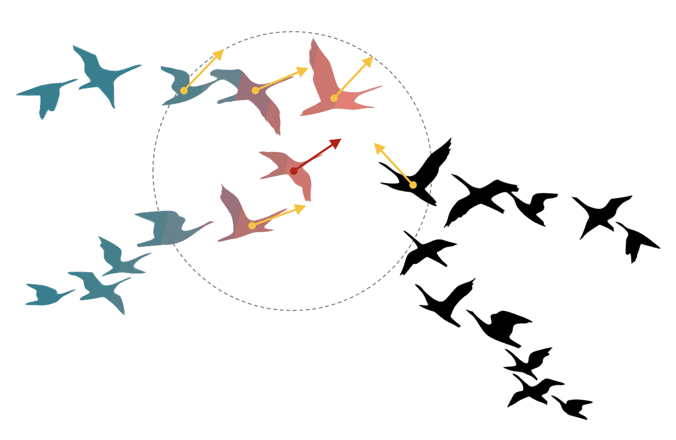
Figure 2: A bird is influenced by its neighbors within distance $r$.

We rewrite the map of the velocity dynamics (1) in matrix form, $v(t+1)=P_{t}v(t)$, for $t\geq 0$, where $v(t)$ is an $n$-by-3 matrix with each row indicating a velocity vector. We have $P_{t}=Q^{-1}M_{t}$, where $Q=\hbox{diag}(q)$, $q_{i}=1/a_{i}$, and

$$(M_{t})_{ij}=\begin{cases}\,\,\text{$1/a_{i}-|\mathcal{N}_{i}(t)|$ \ if $i=j$}\\ \,\,\text{1 \ if $(i,j)\in G_{t}$ and $i\neq j$}\\ \,\,\text{0 \ else.}\end{cases}$$

Note that $\bar{q}:=\|q\|_{1}^{-1}q$ is the joint stationary distribution and $q=M_{t}\mathbf{1}\leq\mathbf{1}/\rho$, where $\rho:=\min_{i}a_{i}\in(0,1/2]$. Each nonzero entry in row $i$ of $P_{t}$, being either $a_{i}$ or $1-a_{i}|\mathcal{N}_{i}(t)|\geq a_{i}$, is at least $\rho$. This shows that each one of the three coordinates provides its own reversible averaging system $\mathcal{S}_{j}$ ($j=1,2,3$). The only difference between the systems is their initial states. The $s$-energy of any such system is equal to $\sum_{t}E_{s,t}$, where $E_{s,t}=\sum_{i}l_{i}(t)^{s}$ and $l_{i}(t)$ is the length of the $i$-th block at time $t$. (Recall that a block is an interval formed by the embedded edges.) Let $m$ be the maximum number of flocks and $N_{m,\alpha}$ the number of times $t$ at which some block length $l_{i}(t)$ from at least one of $\mathcal{S}_{j}$ ($j=1,2,3$) is at least $\alpha$. For $0<\alpha<1$, we have $N_{m,\alpha}\leq\inf_{s\in(0,1]}3\alpha^{-s}\mathcal{E}_{m,s}^{\text{\sc rev}}$. Our assumption that $\|v_{i}(0)\|\leq\frac{1}{2}\sqrt{\rho/n}$ for all birds $i$ implies that each of the three systems has variance at most 1. Setting $s=c/\log(1/\alpha)$ and assuming that $\alpha$ is small enough so that $0<s\leq 1$, it follows from Theorem 1.1 (b) that, for (another) constant $c>0$,

$$N_{m,\alpha}\leq c\Big{(}\frac{n^{2}}{\rho}\log\frac{1}{\alpha}\Big{)}^{m}.$$ (2)

2.1.1 Single-flock dynamics

Between two consecutive switches (ie, edge changes), the flocking networks consists of fixed non-interacting flocks. We can analyze them separately. Without loss of generality, assume that $G_{t}$ is a connected, time-invariant graph. We focus on system $\mathcal{S}_{1}$ for convenience. It consists of a single block at each timestep, so the $s$-energy is of the form $\sum_{t}\Delta_{t}^{s}$, where $\Delta_{t}$ is the diameter of the system at time $t\geq 0$. The diameter can never grow; therefore $\Delta_{t}\leq\alpha$ for any $t\geq N_{1,\alpha}$. By (2), it follows that $\Delta_{t}\leq e^{-a\rho t/n^{2}}$, for any $t\geq n^{2}/a\rho$ and a small enough constant $a>0$. Recall that $x(t)$ and $v(t)$ are $n$-by-3 matrices; denote their first column by $y(t)$ and $w(t)$, respectively. Write $y(0)=y$, $w(0)=w$, and $P_{t}=P$. The vector $w(t)=P^{t}w$ tends to $(\bar{q}^{T}w)\mathbf{1}$. Since its coordinates lie in an interval of width $\Delta_{t}$, it follows that $w(t)=(\bar{q}^{T}w)\mathbf{1}+\zeta(t)$, where $\|\zeta(t)\|_{\infty}\leq\Delta_{t}\leq e^{-a\rho t/n^{2}}$. Thus, for some $\gamma,\eta_{t}\in\mathbb{R}^{n}$ and any $t\geq t_{a}$, with

$$t_{a}:=(n^{2}/a\rho)^{2},$$ (3)

we have

$$y(t)=y+\sum_{k=1}^{t}w(k)=y+t(\bar{q}^{T}w)\mathbf{1}+\sum_{k=1}^{t}\zeta(k)=\beta t+\gamma+\eta_{t},$$

where $\beta=(\bar{q}^{T}w)\mathbf{1}$, $\gamma=y+\sum_{k=1}^{\infty}\zeta(k)$, and $\|\eta_{t}\|_{\infty}\leq e^{-b\rho t/n^{2}}$, for constant $b>0$. The same holds true for the other two coordinates, so the birds in the flock fly parallel to a straight line with a deviation from their asymptotic line vanishing exponentially fast. If so desired, it is straightforward to lock the flocks by stipulating that no two birds can lose an edge between them unless their difference in velocity exceeds a small threshold $\theta$; because of the exponential convergence rate, choosing $\theta$ small enough ensures that two birds $i$ and $j$ adjacent in a flock may exceed distance $r$ by only a tiny amount.

2.1.2 Flock fusion

To bound the relaxation time, we begin with an intriguing geometric fact: Far enough into the future, two birds can only come close to each other if their velocities are nearly identical. In other words, encounters at large angles of attack cannot occur over a long time horizon. We begin with a technical lemma: A stationary observer positioned at the initial location of a bird sees that bird move less and less over time; this is because the bird flies increasingly in the direction of the line of sight.

Lemma 2.2

$\!\!\!.\,\,$ There is a constant $c=c(\varepsilon_{o})$ such that, for any $i$ and $t>1$,

$$\Big{\|}\,v_{i}(t)-\frac{1}{t}\bigl{(}x_{i}(t)-x_{i}(0)\bigr{)}\,\Big{\|}\leq cn^{2(m+2)}\left(\frac{1}{\rho}\right)^{m+1}\left(\frac{\log t}{t}\right)\,.$$

Proof. For notational convenience, we set $i=1$ and we denote by $y_{j}(t)$ (resp. $w_{j}(t)$) the first coordinate of $x_{j}(t)$ (resp. $v_{j}(t)$). The line-of-sight direction of bird 1 is given by $\frac{1}{t}\bigl{(}x_{1}(t)-x_{1}(0)\bigr{)}$. Along the first coordinate axis, this gives

$$u:=\frac{1}{t}\bigl{(}y_{1}(t)-y_{1}(0)\bigr{)}=\frac{1}{t}\sum_{k=1}^{t}w_{1}(k).$$ (4)

Consider the difference $\delta:=u-w_{1}(t)$. We can define the corresponding quantity for each of the other two directions and assume that $\delta$ has the largest absolute value among the three of them. By symmetry, we can also assume that $\delta\geq 0$; therefore

$$\bigl{\|}v_{1}(t)-\hbox{$\frac{1}{t}$}\bigl{(}x_{1}(t)-x_{1}(0)\bigr{)}\bigr{\|}\leq\sqrt{3}\,\delta.$$ (5)

The proof of the lemma rests on showing that, if $\delta$ is too large, some bird $l$ must be at a distance greater than 2 from bird $1$ at time 0, which has been ruled out. To identify the far-away bird $l$, we start with $l=1$ at time $t$, and we trace the evolution of its flock backwards in time, always trying to move away from bird 1, if necessary by switching bird $l$ with a neighbor. This is possible because of two properties, at least one of which holds at any time $k$: (i) bird $l$ flies nearly straight in the time interval $[k,k+1]$; or (ii) bird $l$ is adjacent to a bird $l^{\prime}$ whose velocity points in a favorable direction. In the latter case, we switch focus from $l$ to $l^{\prime}$.

The $s$-energy plays the key role in putting numbers behind these properties. For this reason, we define $\mu_{l}(k)$ as the length of the block of $\mathcal{S}_{1}$ containing $w_{l}(k)$ with respect to the flocking network $G_{k}$. Note that $\mu_{l}(k)$ is the length of an interval that contains the numbers $w_{j}(k)$ for all the birds $j$ in the flock of bird $l$ at time $k$. We define the sequence of velocities $\bar{w}(k)=w_{l}(k)$, for $k=t,t-1,\ldots,1$ and $l=l(k)$. Fix some small $\alpha$ ($0<\alpha\leq\varepsilon_{o}$).

• $\bar{w}(t)\leftarrow w_{1}(t)$   and   $l\leftarrow 1$

• for   $k=t-1,\ldots,1$

• if  $\mu_{l}(k)>\alpha$  then  $l\leftarrow\text{argmin}\left\{\,w_{j}(k)\,|\,j\in N_{l}(k)\,\right\}$

• $\bar{w}(k)\leftarrow w_{l}(k)$

Perhaps the best way to understand the algorithm is first to imagine that the conditional in step [3] never holds: In that case, $l=1$ throughout and we are simply tracing the backward evolution of bird 1. Step [3] aims to catch the instances where the reverse trajectory inches excessively toward the initial position of bird 1. When that happens, $|w_{l}(k+1)-w_{l}(k)|$ is large, hence so is $\mu_{l}(k)$, and step [3] kicks in. We exploit the fact that $w_{l}(k+1)$ is a convex combination of $\bigl{\{}w_{j}(k)\,|\,j\in N_{l}(k)\bigr{\}}$ to update the current bird $l$ to a “better” one. Using summation by parts, we find that

$$\sum_{k=1}^{t}\bar{w}(k)=t\bar{w}(t)-\sum_{k=1}^{t-1}k\bigl{(}\bar{w}(k+1)-\bar{w}(k)\bigr{)}.$$ (6)

Let $R$ be the set of times $k$ that pass the test in step [3] and $S$ the set of switches (ie, network changes). An edge creation entails a block of length $\varepsilon_{o}/\sqrt{3}$ or more in at least one of $\mathcal{S}_{j}$ ($j=1,2,3$). The steps witnessing edge deletions outnumber those seeing edge creations by at most a factor of $\binom{n}{2}$. Pick any two consecutive switches and let $I$ be the time interval between them. Each flock remains invariant during $I$; thus $|R\cap I|\leq N_{1,\alpha}$; hence

$$|S|\leq n^{2}N_{m,\varepsilon_{o}/\sqrt{3}}\hskip 19.91684pt\text{and}\hskip 19.91684pt|R|\leq(N_{1,\alpha}+1)|S|.$$ (7)

Because of the single-flock invariance, the diameter of $\mathcal{S}_{1}$ during $I$ can never increase; therefore $J=I\setminus R$ consists of a single time interval. If $k\in J$, then $|\bar{w}(k+1)-\bar{w}(k)|=|w_{l}(k+1)-w_{l}(k)|\leq\mu_{l}(k)\leq\alpha$ and, by Theorem 1.1 (b), $\sum_{k\in J}|\bar{w}(k+1)-\bar{w}(k)|\leq\sum_{k\in J}E_{1,k}\leq\alpha\,\mathcal{E}_{1,1}^{\text{\sc rev}}=O(\alpha n^{2}/\rho)$; hence

$$\sum_{k\in\{1,\ldots,t-1\}\setminus R}\bigl{|}\bar{w}(k+1)-\bar{w}(k)\bigr{|}=O(\alpha n^{2}|S|/\rho).$$ (8)

Let $l^{\prime}$ be the value of $l$ in the final assignment $\bar{w}_{l}(1)\leftarrow w_{l}(1)$ in step [4]. Since $\bar{w}(k+1)\geq\bar{w}(k)$ for $k\in R$ and $\bar{w}(t)=w_{1}(t)$, it follows from (6, 8) and $r\leq 1$ that

$$\begin{split}y_{l^{\prime}}(0)-y_{1}(0)&\geq\bigl{(}y_{1}(t)-y_{1}(0)\bigr{)}+\bigl{(}y_{l^{\prime}}(0)-y_{1}(t)\bigr{)}\geq tu-\sum_{k=1}^{t}\bar{w}(k)-r|R|\\ &\geq t\delta+\sum_{k=1}^{t-1}k\bigl{(}\bar{w}(k+1)-\bar{w}(k)\bigr{)}-|R|\geq t\delta-O(t\alpha n^{2}|S|/\rho)-|R|.\end{split}$$ (9)

We set $\alpha=\varepsilon_{o}/t$. Noting that $y_{l^{\prime}}(0)-y_{1}(0)\leq 2$, the lemma follows from (2, 5, 7) and

$$\delta\leq dn^{2(m+2)}\left(\frac{1}{\rho}\right)^{m+1}\left(\log\frac{1}{\varepsilon_{o}}\right)^{m}\frac{\log(t/\varepsilon_{o})}{t}\,.$$

for constant $d>0$. $\Box$

2.1.3 Stabilization

By Lemma 2.2, for a large enough constant $C=C(\varepsilon_{o})$, after time $t>t_{0}$, where

$$t_{o}:=Cmn^{2(m+2)}\left(\frac{1}{\rho}\right)^{m+1}\log\frac{n}{\rho},$$

no bird’s velocity differs from its line-of-sight vector $\omega_{i}=\frac{1}{t}\bigl{(}x_{i}(t)-x_{i}(0)\bigr{)}$ by a vector longer than $\varepsilon_{o}/3$. Suppose that birds $i$ and $j$ are within distance $r$ of each other. By the triangular inequality, $\|\omega_{i}-\omega_{j}\|\leq\frac{1}{t}\|x_{i}(t)-x_{j}(t)\|+\frac{1}{t}\|x_{i}(0)-x_{j}(0)\|\leq(1+r)/t$; therefore,

$$\|v_{i}(t)-v_{j}(t)\|\leq\|v_{i}(t)-\omega_{i}\|+\|\omega_{i}-\omega_{j}\|+\|v_{j}(t)-\omega_{j}\|\leq\varepsilon_{o}.$$

This implies that each flock is time-invariant past time $t_{o}$. By (3), $t_{o}\geq t_{a}$, so the birds within each flock align their velocities exponentially fast from that point on. Theorem 2.1 follows. $\Box$

2.2 Distributed Motion Coordination

In [60], Sugihara and Suzuki introduced an interesting model of pattern formation in a swarm of robots. In their model, the robots can communicate anonymously and adjust their positions accordingly. Assume that their goal is to align themselves along a line segment $ab$. Two robots position themselves manually at the endpoints of the segment while the others attempt to reach $ab$ by linking with their right/left neighbors and averaging their positions iteratively. This setup creates a polygonal line $u_{1}=a,u_{2},\ldots,u_{n-1},u_{n}=b$, where $u_{i}$ is the position $(x_{i},y_{i})$ of robot $i$. The polygonal line converges to $ab$ in the limit. We use the $s$-energy bounds to evaluate the convergence time of the robots. We actually prove a stronger result by generalizing the model in two ways: (i) we consider the case of an arbitrary communication network of robots in 3D, with a subset of vertices pinned to a fixed plane; (ii) the network suffers from stochastic edge failures. Our model trivially reduces to Sugihara and Suzuki’s by projection. Allowing stochastic failures to their motion coordination model is novel.

Let $G$ be a connected (undirected) graph with $n$ vertices labeled in $[n]$ and no self-loops, and let the communication weights $a_{1},\ldots,a_{n}$ be $n$ positive reals such that $a_{i}<1/(d_{i}+1)$, where $d_{i}$ is the degree of vertex $i$. We define $d=\max d_{i}$ and $\rho=\min a_{i}$. For any $t\geq 0$, we define $G_{t}$ by deleting each edge of $G$ with probability $1-p$. We define a (random) stochastic matrix $P_{t}$ for $G_{t}$ as follows:

1. Initialize $P_{t}=0$;

2. If $(i,j)$ is an edge of $G_{t}$, we set $(P_{t})_{ij}=a_{i}$ and $(P_{t})_{ji}=a_{j}$.

3. $(P_{t})_{ii}=1-\sum_{j(j\neq i)}(P_{t})_{ij}$, for all $i$.

Note that every positive entry of $P_{t}$ is at least $\rho$. We embed $G$ in $\mathbb{R}^{3}$ and pin a subset $R$ of $r$ vertices to a fixed plane. We fix the scale by assuming that the embedding lies in the unit cube $[0,1]^{3}$. Without loss of generality, we choose the plane $X=0$. To ensure the immobility of the $r$ vertices, we use symmetrization [14]. This entails attaching to $R$ a copy of $G$ and initializing the embedding of the two copies as mirror-image reflections about $X=0$. This modification increases the number of vertices to $\nu=2n-r$. The sequence $(P_{t})_{t\geq 0}$ is defined by picking a random $G_{t}$ (as defined above) at each step iid.

The vertices of $R$ are embedded in the plane $X=0$ at time 0, where, by symmetry, they reside permanently (but may move within the plane). To assert and measure the attraction of the points to the plane, it suffices to focus on the dynamics along the $X$-axis. Given $x(0)\in[-1,1]^{\nu}$, we have $x(t+1)=P_{t}x(t)$. This gives us a reversible averaging system, with $q=(1/a_{1},\ldots,1/a_{\nu})$; note that symmetrization may increase the degrees by at most a factor of 2; and so $a_{i}$ and hence $\rho$ may have to be scaled down by up to one half. Put $\|y\|_{q}:=\sqrt{\langle y,y\rangle_{q}}$, where $\langle y,z\rangle_{q}:=\sum_{i}q_{i}y_{i}z_{i}$ and

$$D_{t}=\sum_{i}\max_{j:\,(i,j)\in G_{t}}\bigl{(}x_{i}(t)-x_{j}(t)\bigr{)}^{2}.$$

Since $G$ is connected, there is a path $\pi$ connecting the leftmost to the rightmost vertex along the $X$-axis. By the Cauchy-Schwarz inequality,

$$\mathbb{E}\,D_{t}\geq\mathbb{E}\sum_{i=1}^{\nu}\max_{j:(i,j)\in G_{t}}\delta_{ij}^{2} \geq\sum_{i=1}^{\nu}\sum_{j:(i,j)\in G}p\delta_{ij}^{2}/d_{i}$$

$$\geq\frac{p}{d\nu}\Bigl{(}\sum_{(i,j)\in\pi}|\delta_{ij}|\Bigr{)}^{2} \geq\frac{\rho p}{d\nu^{2}}\|x\|_{q}^{2}\,,$$

where $\delta_{ij}=\delta_{ij}(t)=x_{i}(t)-x_{j}(t)$. It follows from Lemma 3.5 (see §3.2 below) that, for $c:=\rho p/(2d\nu^{2})$,

$$\mathbb{E}\,\|Px\|_{q}^{2}\leq\|x\|_{q}^{2}-\frac{1}{2}\,\mathbb{E}\,D_{t}\leq(1-c)\|x\|_{q}^{2}.$$

By Markov’s inequality,

$$\Pr\left[\|Px\|_{q}^{2}\geq\Bigl{(}1-\frac{c}{3}\Bigr{)}\|x\|_{q}^{2}\right]\leq\frac{\mathbb{E}\,\|Px\|_{q}^{2}}{(1-c/3)\|x\|_{q}^{2}}\leq 1-\frac{c}{2}\,.$$

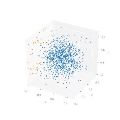
(a) Initially, moving robots are placed randomly in the unit cube.

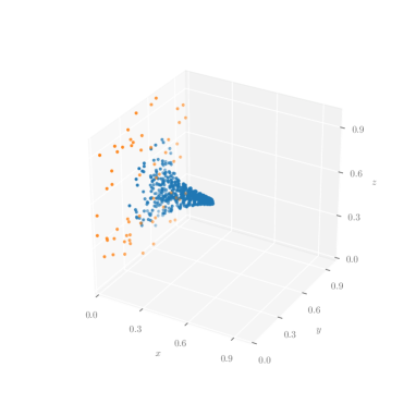
(b) Positions of moving robots after 200 steps.

Figure 3: Simulation of a network of 900 robots in 3D with 60 of them (orange dots) pinned to a fixed plane $X=0$ and the rest (blue dots) are moving. The underlying network $G$ is a 30-by-30 grid graph, with edge failure probability equal to 0.3. The 60 nodes on two opposite sides of the grid are pinned to $X=0$.

Let $l_{1}(t),\ldots,l_{k_{t}}(t)$ be the lengths of the blocks formed by the edges of $G_{t}$ embedded along the $X$-axis. In a slight variant, we define the $s$-energy $E_{s}=\sum_{t\geq 0}E_{s,t}$, where $E_{s,t}=\max_{i=1}^{k_{t}}l_{i}(t)^{s}$. We denote by $W_{s}$ the maximum expected $s$-energy, where the maximum is taken over all initial positions such that $\|x\|_{q}^{2}\leq\nu/\rho$. Since the vertices are embedded in $[-1,1]$ with symmetry about the origin, this applies to the case at hand. Since $q_{i}=1/a_{i}>1$, the initial diameter for $W_{s}$ is at most $\sqrt{2}\,\|x\|_{q}\leq\sqrt{2\nu/\rho}$. (Note that we cannot use 2 as the bound for the diameter since $W_{s}$ only bounds the variance and not the diameter.) By scaling invariance, we have the following recurrence relation:

$$\begin{split}W_{s}&\leq\left(\frac{2\nu}{\rho}\right)^{s/2}+\frac{c}{2}\left(1-\frac{c}{3}\right)^{s/2}W_{s}+\left(1-\frac{c}{2}\right)W_{s}\leq\frac{2^{s+1}\nu^{s/2}}{c\rho^{s/2}\big{(}1-(1-c/3)^{s/2}\big{)}}\\ &=O\left(\frac{\nu^{s/2}}{sc^{2}\rho^{s/2}}\right)=O\left(\frac{dn^{2}}{\rho p}\right)^{2}\frac{(n/\rho)^{s/2}}{s}\,.\end{split}$$

Let $N_{\alpha}$ be the number of times $t$ at which some block length $l_{i}(t)$ is at least $\alpha$. For $0<\alpha<1$, we have $\mathbb{E}\,N_{\alpha}\leq\inf_{s\in(0,1]}\alpha^{-s}W_{s}$. Setting $s=1/\log(n/\rho\alpha^{2})$ yields

$$\mathbb{E}\,N_{\alpha}=O\left(\frac{dn^{2}}{\rho p}\right)^{2}\log\frac{n}{\rho\alpha}\,.$$

Let $K_{\alpha}$ be the number of times $t$ at which there exists an edge $(i,j)\in G_{t}$ whose length $|\delta_{ij}(t)|$ exceeds $\alpha$; obviously, $K_{\alpha}\leq N_{\alpha}$. Let $T_{\alpha}$ be the last time at which the diameter of the system exceeds $\alpha$. For each $t\leq T_{\alpha}$, being a connected graph, $G$ must include an edge $(i,j)$ whose length $|\delta_{ij}(t)|$ exceeds $\alpha/\nu$. That edge belongs to $G_{t}$ with probability $p$; therefore $\mathbb{E}\,K_{\alpha/\nu}\geq p\,\mathbb{E}\,T_{\alpha}$; hence $\mathbb{E}\,T_{\alpha}\leq\frac{1}{p}\mathbb{E}\,N_{\alpha/\nu}$.

Theorem 2.3

$\!\!\!.\,\,$ The robots align themselves within distance $\epsilon<1$ of a fixed plane in expected time $O\bigl{(}d^{2}n^{4}/p^{3}\rho^{2}\bigr{)}\log(n/\rho\varepsilon)$, where $d$ is the maximum degree of the underlying communication network, $n$ is the number of robots, $1-p$ is the probability of edge failure, and $\rho$ is the smallest communication weight.

2.3 The Overton Window Attractor

Following in a long line of opinion dynamics models [11, 22, 23, 31, 34], we consider a collection of $n$ agents, each one holding an opinion vector $x_{i}(t)\in[0,1]^{d}$ at time $t$; we denote by $x(t)$ the $n$-by-$d$ matrix whose $i$-th row corresponds to $x_{i}(t)$. Given a stochastic matrix $P_{t}$, the agents update their opinion vectors at time $t\geq 0$ according to the evolution equation $x(t+1)=P_{t}\,x(t)$. We assume that the last $k$ agents $n-k+1,\ldots,n$ are fixed in the sense that $x_{i}(t)$ remains constant at all times $t\geq 0$. Algebraically, the square block of $P_{t}$ corresponding to the $k$ fixed agents is set to the identity matrix $\mathbb{I}_{k}$. The fixed agents can influence the mobile ones, but not the other way around. The presence of fixed agents (also called “stubborn,” “forceful” or “zealots” in the literature) has been extensively studied [3, 2, 18, 33, 47, 48, 61, 67].

In the context of social networks, the fixed sources may consist of venues with low user influence, such as news outlets, wiki pages, influencers, TV channels, political campaign sites, etc. [19, 32, 38, 42, 53, 64, 68]. We know how the mobile agents migrate to the convex hull of the fixed agents; crucially, we bound the rate of attraction. This provides both a quantitative illustration of the famous Overton window phenomenon as well as a theoretical explanation for why the window acts as an attracting manifold [5, 8, 24, 30, 50]. Interestingly, the emergence of a global attractor does not imply convergence (ie, fixed-point attraction). The mobile agents might still fluctuate widely in perpetuity. The point is that they will always do so within the confines of the global attractor.

To reflect the stochasticity inherent in the choice of sources visited by a user on a given day, we adopt a classic “planted” model: Fix a connected $n$-vertex graph $G$ and two parameters $p\in(0,1]$ and $\rho\in(0,1/2]$. At each time $t\geq 0$, $G_{t}$ is defined by picking every edge of $G$ with probability at least $p$. (No independence is required and $n$ self-loops are included.) We define an $n$-by-$n$ stochastic matrix $P_{t}$ by setting every entry to 0 and updating it as follows:

1. For $i>n-k$, $(P_{t})_{ii}=1$.

2. For $i\leq n-k$, set $(P_{t})_{ij}\geq\rho$ for any $j$ such that $(i,j)$ is an edge of $G_{t}$.

Note that the update is highly nondeterministic. The only two conditions required are that (i) nonzero entries be at least $\rho$ and (ii) each row sum up to 1.

Theorem 2.4

$\!\!\!.\,\,$ For any $\delta,\varepsilon>0$, with probability at least $1-\delta$, all of the agents fall within distance $\varepsilon$ of the convex hull of the fixed agents after a number of steps at most

$$\frac{1}{p\delta}\left(\frac{c}{\rho}\log\frac{dn}{\varepsilon}\right)^{2(n-1)}$$

for constant $c>0$.

Proof. Let $Q_{t}$ be the $h$-by-$h$ upper-left submatrix of $P_{t}$, where $h=n-k$. Note that $Q_{\leq t}:=Q_{t}\cdots Q_{0}$ coincides with the $h$-by-$h$ upper-left submatrix $P_{\leq t}$. Thus, to show that the mobile agents are attracted to the convex hull of the fixed ones, it suffices to prove that $Q_{\leq t}$ tends to $\mathbf{0}_{h\times h}$. To do that, we create an averaging system consisting of $h+1$ agents embedded in $[0,1]$ and evolving as $y(t+1)=A_{t}\,y(t)$, where: $y(t)\in\mathbb{R}^{h+1}$; $y_{h+1}(0)=0$; $v=(\mathbb{I}_{h}-Q_{t})\mathbf{1}_{h}$; and

$$A_{t}=\begin{pmatrix}Q_{t}&v\\ \mathbf{0}_{h}^{T}&1\end{pmatrix}.$$

The system lacks the requisite symmetry to qualify as a general averaging system, so we again use symmetrization [14] by duplicating the $h$ mobile agents and initializing the embedding of the two copies as mirror-image reflections about the origin. The new evolution matrix is now $\nu$-by-$\nu$, where $\nu=2h+1$:

$$B_{t}=\begin{pmatrix}Q_{t}&v&\mathbf{0}_{h\times h}\\ u&1-2\|u\|_{1}&u\\ \mathbf{0}_{h\times h}&v&Q_{t}\end{pmatrix}.$$

We define the row vector $u\in\mathbb{R}^{h}$ by setting its $i$-th coordinate to $\rho$ if $v_{i}>0$ and $0$ otherwise. We require that $1-2\|u\|_{1}\geq\rho$; hence $\rho\leq 1/(2d_{t}+1)$, where $d_{t}$ is the number of mobile agents (among the $h$ of them) adjacent in $G_{t}$ to at least one fixed agent. This condition is easily satisfied by setting $\rho\leq 1/2n$. The evolution follows the update: $z(t+1)=B_{t}\,z(t)$, where $z(t)\in[-1,1]^{\nu}$ and $z_{h+1}(0)=0$.

Let $G^{*}$ be the augmented $\nu$-vertex graph formed from $G$ and let $G_{t}^{*}$ be its subgraph selected at time $t$. Note that, via $z(t)$, these graphs are embedded in $[-1,1]^{\nu}$. If $\Delta_{t}$ denotes the length of the longest edge of $G^{*}$ at time $t$ and $T_{\alpha}$ is the last time at which the diameter of the system is at least $\alpha$, then $\Delta_{t}\geq\alpha/\nu$ for all $t\leq T_{\alpha}$ because $G^{*}$ is connected. The longest edge in $G^{*}$ (with ties broken alphabetically) appears in $G_{t}^{*}$ with probability at least $p$. Fix $s\in(0,1]$ and define the random variable $\chi_{t}$ to be $\Delta_{t}^{s}$ if the longest edge of $G$ at time $t$ is in $G_{t}$ and $0$ otherwise. By [16], the maximum $s$-energy is at most $\mathcal{E}_{s}\leq 2^{s}(3/\rho s)^{\nu-1}$; hence

$$\mathbb{E}\,T_{\alpha}\leq\left(\frac{\nu}{\alpha}\right)^{s}\mathbb{E}\sum_{t\geq 0}\Delta_{t}^{s}\leq\frac{1}{p}\left(\frac{\nu}{\alpha}\right)^{s}\mathbb{E}\sum_{t\geq 0}\chi_{t}\leq\frac{1}{p}\left(\frac{\nu}{\alpha}\right)^{s}\mathcal{E}_{s}\leq\frac{2}{p}\left(\frac{\nu}{\alpha}\right)^{s}\left(\frac{3}{\rho s}\right)^{\nu-1}.$$

Minimizing the right-hand side over all $s\in(0,1]$ yields

$$\mathbb{E}\,T_{\alpha}\leq\frac{6}{p}\left(\frac{3}{\rho}\log\frac{2n-1}{\alpha}\right)^{2(n-1)}.$$

By Markov’s inequality, $\Pr\,\bigl{[}\,T_{\alpha}\geq t_{\delta}\,\bigr{]}\leq\delta$, where

$$t_{\delta}:=\frac{6}{p\delta}\left(\frac{3}{\rho}\log\frac{2n-1}{\alpha}\right)^{2(n-1)}\,.$$ (10)

This implies that $\|Q_{\leq t}\,\mathbf{1}_{h}\|_{\infty}\leq\alpha$, for all $t>t_{\delta}$, with probability at least $1-\delta$. In other words, for any such $t$, it holds that, for $i\leq h$,

$$q:=\sum_{j=1}^{h}(P_{\leq t})_{ij}=\sum_{j=1}^{h}(Q_{\leq t})_{ij}\leq\alpha.$$

Trivially, $x_{i}(t+1)=q\tilde{u}+(1-q)\tilde{v}$, where

$$\tilde{u}=\frac{1}{q}\sum_{j=1}^{h}(P_{\leq t})_{ij}x_{j}(0)\hskip 17.07182pt\text{and}\hskip 17.07182pt\tilde{v}=\frac{1}{1-q}\sum_{j=h+1}^{n}(P_{\leq t})_{ij}x_{j}(0).$$

Observing that $\tilde{v}$ lies in the convex hull of the fixed agents, we form the difference $x_{i}(t+1)-\tilde{v}=q(\tilde{u}-\tilde{v})$ and note that the distance from $x_{i}(t+1)$ to the hull is bounded by $q\|\tilde{u}-\tilde{v}\|_{2}\leq\alpha\sqrt{d}$. Setting $\alpha=\varepsilon/\sqrt{d}$ completes the proof. $\Box$

We can extend this result so as to relate convergence to connectivity. We now produce the random graph $G_{t}$ from fixed connected $G$ as we did above, but if this results in a graph with more than $m$ connected components, we add random edges picked uniformly from $G$ until the number of components drops to $m$. Using Theorem 1.1 (a) in the proof above leads to a more refined bound:

Theorem 2.5

$\!\!\!.\,\,$ For any $\delta,\varepsilon>0$, with probability at least $1-\delta$, all of the agents fall within distance $\varepsilon$ of the convex hull of the fixed agents in time bounded by

$$\frac{c}{p\delta}\left(\frac{1}{\rho}\right)^{2(n-1)}\left(mn\log\frac{dn}{\varepsilon}\right)^{2m-1},$$

for constant $c>0$. This assumes that no graph used in the process has more than $m$ connected components.

Proof. By Theorem 1.1 (a), we know that $\mathcal{E}_{m,s}\leq(b/s)^{m}(1/\rho)^{n-1}$, for any $s\in(0,1]$, where $b=O(mn)$. The previous proof leads us to update (10) into:

$$t_{\delta}:=\frac{c}{p\delta}\left(\frac{1}{\rho}\right)^{2(n-1)}\left(mn\log\frac{n}{\alpha}\right)^{2m-1}\,,$$

for constant $c>0$, from which the theorem follows. $\Box$

3 The Proofs

3.1 General averaging systems: Theorem 1.1 (a)

An averaging system is a special case of a twist system [16]. The latter is easier to analyze so we turn our attention to it. As opposed to an averaging system, where the next step is uniquely specified, a twist system is nondeterministic. Instead of a fixed rule spelling out the chronological transitions, we are given constraints at each timestep, and any transition that conforms to them is valid.

Relabel the agents so their positions $x_{1}\leq\cdots\leq x_{n}$ appear in sorted order at time $t$. A twist system moves them to positions $y_{1}\leq\cdots\leq y_{n}$ at time $t+1$ in such a way that

$$(1-\rho)x_{u}+\rho x_{\min\{i+1,v\}}\leq y_{i}\leq\rho x_{\max\{i-1,u\}}+(1-\rho)x_{v},$$ (11)

for any $i$ in $[u,v]$ and $y_{i}=x_{i}$ otherwise. We repeat this step indefinitely. Twist systems are highly nondeterministic. At each step, a new interval $[u,v]\subseteq[n]$, called a block, is picked and the agents’ motion is only constrained by (11) and the need to maintain their ranks (ie, agents never cross). It is not entirely obvious that twist systems should always exist: in other words, that the constraints imposed in (11) are always satisfiable. This is a direct consequence of Lemma 3.1, which we state and prove below.

For the purposes of this work, we extend the concept to $m$-twist systems by stipulating, at each time $t$, a partition of $[n]$ into up to $m_{t}$ blocks $[u_{t,l},v_{t,l}]$ ($1\leq l\leq m_{t}\leq m$). Each agent is now subject to (11) within its own enclosing block. We define the $s$-energy $E_{s}^{\text{\sc tw}}$ of a twist system as we did with an averaging system by adding together the $s$-th powers of all the block lengths. We use the same notation with the addition of the superscript tw.

Lemma 3.1

$\!\!\!.\,\,$ An averaging system with at most $m$ connected components at any time can be interpreted as an $m$-twist system with the same $s$-energy.

Proof. Fix an averaging system and let $(x_{i})_{i=1}^{n}$ and $(y_{i})_{i=1}^{n}$ be the positions of the agents at times $t$ and $t+1$, given in nondecreasing order. We denote by $x_{i}^{\prime}$ the position of agent $i$ at time $t+1$. Let $[x_{u},x_{v}]$ be a block at time $t$ (ie, an interval of the union of the embedded edges of $G_{t}$). Pick $k<v$ and write $z=\rho x_{k}+(1-\rho)x_{v}$. All the diagonal elements of $P_{t}$ are at least $\rho$; hence $x^{\prime}_{i}\leq z$, for all $i\leq k$, and $y_{k}\leq z$. In fact, we even have $y_{k+1}\leq z$. Indeed, the embedded edges of $G_{t}$ cover all of $[x_{u},x_{v}]$, so at least one of them, call it $(l,r)$, must join $[u,k]$ to $[k+1,v]$; hence $x^{\prime}_{r}\leq z$. Our claim follows. This proves that, for all $i\in(u,v]$, $y_{i}\leq\rho x_{\max\{i-1,u\}}+(1-\rho)x_{v}$. We omit the case $i=u$ and the mirror-image inequality, which repeat the same argument. Summing up all the powers $(x_{v}-x_{u})^{s}$ shows the equivalence between the two $s$-energies. $\Box$

We may assume that the agents stay within $[0,1]$. We begin with the bound $\mathcal{E}_{m,1}\leq\mathcal{E}_{m,1}^{\text{\sc tw}}\leq 3en(1/\rho)^{\lfloor n/2\rfloor}$.

Case $s=1$

We prove a stronger result by bounding $K_{t}(z)\!:=\sum_{k=1}^{n}\left(x_{v(k)}-x_{k}\right)z^{k}$, where $v(k)=v_{t,l}$ for $l$ such that $k\in[u_{t,l},v_{t,l}]$. As usual, $0\leq x_{1}\leq\cdots\leq x_{n}\leq 1$ denotes the sorted positions of the agents at time $t$; we omit $t$ for convenience but it is understood throughout. We define the weighted $1$-energy $K(z)=\sum_{t\geq 0}K_{t}(z)$ and, finally, $\mathcal{K}(z)=\sup K(z)$. As long as $z\geq 1$, the $1$-energy is obviously dominated by its weighted version. We improve this crude bound via a symmetry argument:

Lemma 3.2

$\!\!\!.\,\,$ For any $z\geq 1$, $\mathcal{E}_{m,1}^{\text{\sc tw}}\leq 2z^{-\nu}\,\mathcal{K}(z)$, where $\nu=\lceil n/2\rceil$.

Proof. We define the mirror image of $K_{t}$ as $\bar{K}_{t}(z)=\sum_{k=1}^{n}\left(x_{k}-x_{u(k)}\right)z^{n-k+1}$, where $u(k)$ is the left counterpart of $v(k)$. We have

$$\begin{split}E_{1,t}^{\text{\sc tw}}&\leq\sum_{k\leq\nu}\left(x_{k}-x_{u(k)}\right)+\sum_{k\geq\nu}\left(x_{v(k)}-x_{k}\right)\\ &\leq z^{-\nu}\sum_{k\leq\nu}\left(x_{k}-x_{u(k)}\right)z^{n-k+1}+z^{-\nu}\sum_{k\geq\nu}\left(x_{v(k)}-x_{k}\right)z^{k}\\ &\leq z^{-\nu}\bigl{(}\bar{K}_{t}(z)+K_{t}(z)\bigr{)}.\end{split}$$

Because $\mathcal{K}(z)=\sup K(z)$, the lemma then follows by summing up over all $t\geq 0$. $\Box$

We define the polynomial $P_{t}(z)=\sum_{k=1}^{n}x_{k}z^{k}$ for $z>1/\rho$ and exploit two simple but surprising facts: $P_{t}(z)$ cannot increase over time; and, at each step, the drop from $P_{t}(z)$ to $P_{t+1}(z)$ is at least proportional to $K_{t}(z)$. Thus, we develop a discrete version of the inference: $dP_{t}/dt\leq-cK_{t}$ implies

$$\int_{t\geq 0}cK_{t}\leq-\int_{t\geq 0}\frac{dP_{t}}{dt}\leq P_{1}\,.$$

Lemma 3.3

$\!\!\!.\,\,$ For any $z>1/\rho$, $P_{t}(z)-P_{t+1}(z)\geq(\rho z-1)K_{t}(z)$.

Proof. The inequality is additive in the number of blocks so we can assume there is a single block $[u,v]$ at time $t$. Using the notation of (11), we have $y_{k}\leq\rho x_{\max\{k-1,u\}}+(1-\rho)x_{v}$; hence

$$\begin{split}P_{t}(z)-P_{t+1}(z)&=\sum_{k=u}^{v}(x_{k}-y_{k})z^{k}\geq\sum_{k=u}^{v}\left(x_{k}-\rho x_{\max\{k-1,u\}}-(1-\rho)x_{v}\right)z^{k}\\ &\geq(\rho-1)(x_{v}-x_{u})z^{u}+\sum_{k=u+1}^{v}\rho(x_{v}-x_{k-1})z^{k}-\sum_{k=u+1}^{v}(x_{v}-x_{k})z^{k}\\ &\geq(\rho-1)(x_{v}-x_{u})z^{u}+\sum_{k=u}^{v-1}\rho z(x_{v}-x_{k})z^{k}-\sum_{k=u+1}^{v}(x_{v}-x_{k})z^{k}\\ &\geq(\rho-1)(x_{v}-x_{u})z^{u}+\sum_{k=u}^{v}(\rho z-1)(x_{v}-x_{k})z^{k}+(x_{v}-x_{u})z^{u}\\ &\geq(\rho z-1)K_{t}(z)+\rho(x_{v}-x_{u})z^{u}.\end{split}$$

$\Box$

The lemma implies that

$$(\rho z-1)K(z)=\sum_{t\geq 0}(\rho z-1)K_{t}(z)\leq P_{0}(z)\leq\sum_{k=1}^{n}z^{k}=\frac{z^{n+1}-z}{z-1}\,.$$ (12)

With $z=(1+\varepsilon)/\rho$, $\varepsilon=1/(n-\nu+1)$, and $n>2$, we find that

$$z^{-\nu}K(z)\leq\frac{z^{n}-1}{(z-1)(\rho z-1)z^{\nu-1}}\leq 2\rho^{\nu-n}e^{(n-\nu+1)\varepsilon}/\varepsilon\leq 2e(n-\nu+1)\rho^{\nu-n}\leq\frac{3en}{2}\rho^{\nu-n}.$$

The case $s=1$ of Theorem 1.1 (a) follows immediately from Lemma 3.2. Finally, for $n=2$, we verify that $\mathcal{E}_{m,1}^{\text{\sc tw}}=\sum_{k\geq 0}(1-2\rho)^{k}=1/2\rho$. $\Box$

Case $s<1$

The previous argument relied crucially on the linearity of the $1$-energy. If $s<1$, the $s$-energy gives more relative weight to small lengths, so we need a different strategy to keep the scales separated. We omit the superscript tw below but it is understood. We use a threshold $\delta$ which, though set to $1/3$, is best kept as $\delta$ in the notation.

A recurrence relation.   Let $T_{\delta}$ be the number of steps at which the diameter remains above $1-\delta$; note that these steps are consecutive and $T_{\delta}$ might be infinite. By scaling, we find that $E_{s}\leq F_{\!s}+(1-\delta)^{s}E_{s}$, where $F_{\!s}=\sum_{t\leq T_{\delta}}E_{s,t}$. Since $(1-\delta)^{s}\leq 1-\delta s$, for $\delta,s\in[0,1]$, we have

$$E_{s}\leq(\delta s)^{-1}F_{\!s}.$$ (13)

If $m=1$, then $(1-\delta)F_{\!s}\leq(1-\delta)T_{\delta}\leq F_{1}\leq\mathcal{E}_{1,1}$. Thus, by (13) and the previous section,

$$\mathcal{E}_{1,s}\leq\frac{3en}{\delta(1-\delta)}(1/s)(1/\rho)^{\lfloor n/2\rfloor}.$$ (14)

We consider the case $m>1$. Fix $t\leq T_{\delta}$; if $m_{t}>1$, let $j$ maximize $x_{j+1}(t)-x_{j}(t)$ over all $j=v_{i}$ and $i<m_{t}$ (break ties by taking the smallest $j$). This corresponds to the maximum distance between consecutive blocks. For this reason, we call $(j,j+1)$ the max-gap at time $t$. We say that $t$ is ungapped if $m_{t}=1$ or $x_{j+1}(t)-x_{j}(t)\leq\delta/m$; it is gapped otherwise. Assuming that $t$ is gapped, let $(j,j+1)$ be its max-gap and write $\zeta_{t}=\min_{k}\bigl{\{}\,t<k\leq T_{\delta}\,|\,\exists\,l:u_{k,l}\leq j<v_{k,l}\,\bigr{\}}$: If the set is empty, we set $\zeta_{t}=T_{\delta}$; else $l$ is unique and we denote it by $l_{t}$. We call the interval $[t,\zeta_{t}]$ a span and the block $l_{t}$, if it exists, its cap. We note that $x_{j+1}(k)-x_{j}(k)$ cannot decrease during the times $k=t,\ldots,\zeta_{t}$. This shows that a cap covers a length greater than $\delta/m$.

We begin with a few words of intuition. The energetic contribution of an ungapped time $t$ is easy to account for: It is at most $m$. On the other hand, the $1$-energy is at least the diameter minus the added length of the gaps between blocks, which amounts to at least $1-2\delta\geq 1/3$; in other words, $E_{s,t}\leq 3mE_{1,t}$. Summing up over all ungapped times and plugging in our bound for $s=1$ gives us the desired result. Accounting for gapped times is more difficult, as it requires dealing with small scales. If we had only one span, we could simply split the system into two decoupled subsystems and set up a recurrence relation. The problem is that the presence of $k$ capped spans would force us to repeat the recursion $k-1$ times. With no apriori bound on $k$, this approach is not too promising. Instead, we make a bold move: We argue that, because a cap is longer than $\delta/m$, its own 1-energy contribution (ie, its length) is large enough to “pay” for the $s$-energy of its entire span. This is not quite right, of course, but one can fix the argument by using the weighted 1-energy of the cap and upscaling it suitably. Once again, this reduces the problem to the case $s=1$, so our method is, in effect, a linearization. Here is the proof.

We partition the times between 0 and $T_{\delta}$ into two subsets $\mathcal{G}$ and $\mathcal{U}\!:=[0,T_{\delta}]\setminus\mathcal{G}$, each one supplied with its own energetic accounting scheme. We form $\mathcal{G}$ by greedily extracting a maximal set of nonoverlapping spans and taking their union.

• $\mathcal{G}\leftarrow\emptyset$ and $t^{\prime}\leftarrow 0$;

• if $t\leftarrow\min\,\bigl{\{}\,\text{gapped }i\,|\,t^{\prime}\leq i\leq T_{\delta}\,\bigr{\}}$ exists

• then $\mathcal{G}\leftarrow\mathcal{G}\cup\bigl{\{}\,i\,|\,t\leq i\leq\zeta_{t}\,\bigr{\}}$;

• if $\zeta_{t}<T_{\delta}$ then $t^{\prime}=\zeta_{t}+1$; go to 2;

We postulate that, for any $0<s\leq 1$, and any number of agents $j\leq n$,

$$\mathcal{E}_{m,s}\leq c_{m}(1/s)^{m}(1/\rho)^{j-1}\,,$$ (15)

and we derive a recurrence relation for $c_{m}$ (for given $n$).

• Accounting for $\mathcal{G}$: In line 3, let $k=\zeta_{t}$ and $(j,j+1)$ be the corresponding max-gap. Suppose that the span $[t,k]$ is capped. The absence of an interval including $j$ and $j+1$ during $[t,k-1]$ implies that $\sum_{t\leq l\leq k}E_{s,l}\leq L+R+m$, where $L$ and $R$ denote the $s$-energy of systems with at most $m-1$ connected components. For reasons we address below, we may assume that $L$ is dominant; hence $R\leq L\leq\mathcal{E}_{m-1,s}$. It follows that

  $$\sum_{l=t}^{k}E_{s,l}\leq 2\mathcal{E}_{m-1,s}+m\leq 3c_{m-1}(1/s)^{m-1}(1/\rho)^{j-1}.$$ (16)

  Note that we (safely) assume $c_{m-1}\geq m$. Using the shorthand $v$ for $v_{k,l_{t}}$, we have $x_{v}(k)-x_{j}(k)\geq x_{j+1}(k)-x_{j}(k)\geq x_{j+1}(t)-x_{j}(t)>\delta/m$. We add the artificial multiplier $x_{v}(k)-x_{j}(k)$ to (16) to make the right-hand side resemble $K(z)$. Recall that $\delta=1/3$; assuming that $z>1/\rho$ from now on, we have

  $$\sum_{l=t}^{k}E_{s,l}\leq B\bigl{(}x_{v}(k)-x_{j}(k)\bigr{)}z^{j},\hskip 11.38092pt\text{\small{with}}\hskip 5.69046ptB=9c_{m-1}m\rho(1/s)^{m-1}$$ (17)

  The set $\mathcal{G}$ is a union of spans. If $\zeta_{t}=T_{\delta}$, the last span might not be capped. If so, remove it from $\mathcal{G}$ and call the resulting set $\mathcal{G}^{\prime}$. Summing up, we find that $\sum_{t\in\mathcal{G}^{\prime}}E_{s,t}\leq B\sum_{t\in\mathcal{G}^{\prime}}K_{t}(z)$. If the last span is uncapped then $\zeta_{t}=T_{\delta}$ and no block contains both $j$ and $j+1$ in the span $[t,T_{\delta}]$. The $s$-energy expended in that span is thus of the form $L+R\leq 2\mathcal{E}_{m-1,s}$.

• Accounting for $\mathcal{U}$: Only ungapped times belong to $\mathcal{U}$, so the 1-energy at time $t\in\mathcal{U}$ is at least $1-\delta-(m_{t}-1)\delta/m\geq 1/3$. On the other hand, $E_{s,t}\leq m\leq 3mE_{1,t}\leq 3m\rho K_{t}(z)\leq BK_{t}(z)$.

Set $z=(1+\varepsilon)/\rho$, for $\varepsilon>0$. Putting all of our bounds together, we have

$$\begin{split}F_{\!s}=\sum_{t\leq T_{\delta}}E_{s,t}&\leq B\sum_{t\in\mathcal{G}^{\prime}}K_{t}(z)+2\mathcal{E}_{m-1,s}+B\sum_{t\in\mathcal{U}}K_{t}(z)\\ &\leq 2c_{m-1}\,(1/s)^{m-1}(1/\rho)^{n-1}+BK(z).\end{split}$$

Actually, the exponent to $1/\rho$ can be reduced to $n-2$, but this is immaterial. By (12),

$$BK(z)\leq 18c_{m-1}(1/s)^{m-1}(1/\rho)^{n-1}e^{(n+1)\varepsilon}(m/\varepsilon).$$

Setting $\varepsilon=1/(n+1)$ gives us, for some constant $d>0$,

$$F_{\!s}\leq c_{m-1}(dmn)(1/s)^{m-1}(1/\rho)^{n-1}.$$

We tie up the loose ends by arguing that it was legitimate to assume that $L\geq R$. The point is that individual values of $L$ and $R$ do not matter: only their sums do. Thus, if the $R$s outweigh the $L$s, we restore the dominance of the $L$s by flipping the system around. Finally, by (13), $E_{s}\leq(3/s)F_{\!s}$; and so, by (14), Theorem 1.1 (a) follows from the recurrence: $c_{1}=O(n)$ and $c_{m}\leq 3dmnc_{m-1}$, for $m>1$. $\Box$

Lower bounds for twist systems.

We begin with the case $m=1$. Assume that $n=2k+1$. At time $t=1$, we have $x_{k}=-x_{-k}=1/2$ and $x_{i}=-x_{-i}=\frac{1}{2}(1-\rho^{i})$, for $0\leq i<k$ and $\rho$ small enough. For $t>1$, we set $x_{i}(t)=(1-\rho^{k})x_{i}(t-1)$. The agents are labeled $-k,\ldots,k$ from left to right. It is easily verified that this constitutes a twist system for the block $[-k,k]$ with initial unit diameter. The $s$-energy $E$ is $\bigl{(}1-\rho^{k}\bigr{)}^{s}E+1$ so, for constant $c>0$,

$$E\geq(c/s)(1/\rho)^{\lfloor n/2\rfloor}.$$ (18)

If $n=2k$, we set $x_{k}=-x_{-k}=1/2$ and $x_{i}=-x_{-i}=\frac{1}{2}(1-2\rho^{i})$, for $1\leq i<k$. For $t>1$, we set $x_{i}(t)=(1-2\rho^{k})x_{i}(t-1)$ and rederive (18).

For the general case, we describe the evolution of an $m$-block twist system with $n$ agents, and denote its $s$-energy by $F(n,m)$: It is assumed that $n-1$ agents are positioned at $0$ at time 1 and the last one is at position $1$. If $m=1$, we apply the previous construction after shifting the initial interval from $[-0.5,0.5]$ to $[0,1]$. The initial positions still do not match, but we note that, in a single step, we can move the agents anywhere we want in the interval $[\rho,1-\rho]$ while respecting the constraints of a twist system. This gives us $F(n,1)=1+(1-2\rho)^{s}E$. By adjusting the constant $c$ in (18), the same lower bound still holds.

For $m>1$, at time $1$, we move the agents $n-1$ and $n$ to positions $\rho$ and $1-\rho$, respectively, and we leave the others (if any) at position 0. We then use an $(m-1)$-block twist system recursively for the agents $1,\ldots,n-1$. This brings these agents to a common position in $[0,\rho]$. This gives us the recurrence relation: $F(n,m)\geq 1+\rho^{s}F(n-1,m-1)+(1-2\rho)^{s}F(n,m)$; hence, by induction, for constant $c>0$,

$$F(n,m)\geq(c/s)^{m}\rho^{(m-1)s}(1/\rho)^{\lfloor(n+m-1)/2\rfloor}.$$ (19)

The $s$-energy is often used for small $s$, so we state the case of $s=O\bigl{(}1/m\log\frac{1}{\rho}\bigr{)}$, which matches the bound of Theorem 1.1 (a) for $m=n-1$.

Theorem 3.4

$\!\!\!.\,\,$ $\mathcal{E}_{m,s}^{\text{\sc tw}}\geq(c/s)^{m}(1/\rho)^{\lfloor(n+m-1)/2\rfloor}$, for constant $c>0$, small enough $\rho$ and $s=O\bigl{(}1/m\log\frac{1}{\rho}\bigr{)}$.

3.2 Reversible averaging systems: Theorem 1.1 (b)

Recall that, in a reversible averaging system rev, $P_{t}=\text{diag}(q)^{-1}M_{t}$, where $M_{t}$ is symmetric with nonzero entries at least 1 and $q=M_{t}\mathbf{1}\preceq\mathbf{1}/\rho$. The vector $q$ is proportional to the stationary distribution of the Markov chain induced by $P_{t}$. By reversibility, we have $q_{i}(P_{t})_{ij}=q_{j}(P_{t})_{ji}$. Write $\langle x,y\rangle_{q}:=\sum_{i}q_{i}x_{i}y_{i}$ and $\|x\|_{q}^{2}:=\langle x,x\rangle_{q}$. The (scaled) variance defined in §1 can be rewritten as $\|x-\hat{x}\,\|_{q}^{2}$ where $\hat{x}=\|q\|_{1}^{-1}\langle x,\mathbf{1}\rangle_{q}\mathbf{1}$ and $x$ is shorthand for $x(0)$. The convergence rate of the attracting dynamics is captured by a variant of the Dirichlet form:

$$D_{t}=\sum_{i}\max_{j:\,(i,j)\in G_{t}}\bigl{(}x_{i}(t)-x_{j}(t)\bigr{)}^{2}.$$ (20)

We omit the index $t$ below for clarity.

Lemma 3.5

$\!\!\!.\,\,$  $\|Px\|_{q}^{2}\leq\|x\|_{q}^{2}-D/2\,$, for any $x\in\mathbb{R}^{n}$.

Proof. Write $\delta_{ij}=x_{i}-x_{j}$ and $\mu_{i}=\sum_{j}p_{ij}\,\delta_{ij}$. Fix $i$ and pick any $k$ such that $m_{ik}>0$. By Cauchy-Schwarz and $m_{ii}\geq 1$ (because nonzero entries of $M$ are at least $1$), we have

$$\delta_{ik}^{2} =\bigl{(}(\mu_{i}-\delta_{ii})+(\delta_{ik}-\mu_{i})\bigr{)}^{2}\leq 2(\delta_{ii}-\mu_{i})^{2}+2(\delta_{ik}-\mu_{i})^{2}\leq 2\sum_{j}m_{ij}\,(\delta_{ij}-\mu_{i})^{2};$$

hence,

$$\|x\|_{q}^{2}-\|Px\|_{q}^{2} =\sum_{i}q_{i}x_{i}^{2}-\sum_{i}q_{i}\,\biggl{(}x_{i}+\sum_{j}p_{ij}\delta_{ji}\biggr{)}^{2}=-\sum_{i}q_{i}\,\biggl{(}2x_{i}\sum_{j}p_{ij}\delta_{ji}+\mu_{i}^{2}\biggr{)}$$

$$=\sum_{i}q_{i}\,\biggl{(}\,\sum_{j}p_{ij}\,\delta_{ij}^{2}-\mu_{i}^{2}\,\biggr{)}=\sum_{i,j}m_{ij}\,(\delta_{ij}-\mu_{i})^{2}\geq\frac{1}{2}\sum_{i}\max_{j:m_{ij}>0}\delta_{ij}^{2},$$

with the last equality expressing the identity for the variance: $\mathbb{E}X^{2}-(\mathbb{E}\,X)^{2}=\mathbb{E}[X-\mathbb{E}\,X]^{2}$. $\Box$

Write $G_{\leq t}$ as the union of all the edges in $G_{0},\ldots,G_{t}$, and let $t_{c}$ be the maximum value of $t$ such that $G_{\leq t}$ has fewer connected components than $G_{\leq t-1}$; if no such $t$ , set $t_{c}=0$.

Lemma 3.6

$\!\!\!.\,\,$ If $G_{\leq t_{c}}$ is connected, then $\sum_{t\leq t_{c}}D_{t}\geq\,\rho n^{-2}\,\|x-\hat{x}\,\|_{q}^{2}\,$.

Proof. Let $G_{t_{0}}$ denote the graph over $n$ vertices with no edges. We define $t_{1},\ldots,t_{c}$ as the sequence of times $t$ at which the addition of $G_{t}$ reduces the number of connected components in $G_{\leq t-1}$. At any time $t_{k}$ ($k>0$), the drop $d_{k}$ in the number of components can be achieved by $d_{k}$ edges from $G_{t_{k}}$. Let $F_{k}$ denote such a set of edges: we can always order $F_{k}$ so that every edge in the sequence contains at least one vertex not encountered yet. This shows that the sum of the squared lengths of the edges in $F_{k}$ does not exceed $D_{t_{k}}$. We note that $F:=F_{1}\cup\cdots\cup F_{c}$ forms a collection of $n-1$ edges from (the connected graph) $G_{\leq t_{c}}$ and $F$ spans all $n$ vertices.

Consider the intervals formed by the edges in $F_{k}$ at time $t_{k}$, for all $k\in[c]$. The union of these intervals covers the smallest interval $[a,b]$ enclosing all the vertices at time $0$ (and hence at all times). To see why, pick any $z$ such that $a<z<b$ and denote by $L$ and $R$ the vertices on both sides of $z$ at time $0$. Neither set is empty and, by convexity, both of them remain on their respective side of $z$ until an edge of some $G_{t}$ joins $L$ to $R$. When that happens (which it must since $G_{\leq t_{c}}$ is connected), the joining edge(s) reduce(s) the number of components of $G_{\leq t-1}$ by at least one, so $F$ must grab at least one of them, which proves our claim. Let $l_{1},\ldots,l_{n-1}$ denote the lengths of the edges of $F$ (at the time of their insertion). By Cauchy-Schwarz, $\sum_{t\leq t_{c}}D_{t}\geq\sum_{i=1}^{n-1}l_{i}^{2}\geq(b-a)^{2}/(n-1)$. The lemma follows from the inequalities $\|x-\hat{x}\,\|_{q}^{2}\leq\|q\|_{1}(b-a)^{2}\leq(n/\rho)(b-a)^{2}$. $\Box$

Assume that $G_{\leq t_{c}}$ is connected. By Lemma 3.6 and the telescoping use of Lemma 3.5,

$$\|x\|_{q}^{2}-\|x(t_{c}+1)\|_{q}^{2}\geq\frac{1}{2}\sum_{t=0}^{t_{c}}D_{t}\geq\frac{\rho}{2n^{2}}\,\|x-\hat{x}\,\|_{q}^{2}\,.$$ (21)

Let $U(n,m)$ be the maximum $s$-energy of a rev with at most $n$ vertices and $m$ connected components at any time, subject to the initial condition $\|x-\hat{x}\,\|_{q}^{2}\leq 1$. By shifting the system if need be, we can always assume that $\hat{x}=\mathbf{0}$. By (21), $\|x(t)\|_{q}^{2}$ shrinks by at least a factor of $\alpha:=1-\rho/2n^{2}$ by time $t_{c}+1$. A simple scaling argument shows that the $s$-energy expanded after $t_{c}$ is at most $\alpha^{s/2}U(n,m)$. While $t<t_{c}$ (or if $G_{\leq t_{c}}$ is not connected), the system can be decoupled into two rev systems, each one with fewer than $m$ components. Since $\|x\|_{q}^{2}\leq 1$, we have $|x_{i}|\leq 1$ for each $i$ and the diameter at any time is at most 2; therefore $U(n,m)\leq\alpha^{s/2}U(n,m)+2U(n,m-1)+m2^{s}$. It follows that

$$U(n,m)\leq\frac{2}{1-\alpha^{s/2}}\,\bigl{(}U(n,m-1)+m\,\bigr{)};$$ (22)

hence $U(n,m)=O(n^{2}/\rho s)^{m}$, and Theorem 1.1 (b) follows. $\Box$

A lower bound for reversible systems.

We begin with the case $m=1$. The path graph $G$ over $n$ vertices has an edge $(i,i+1)$ for all $i<n$. The Laplacian $L$ is $\text{diag}(u)-A$, where $A$ is the adjacency matrix of $G$ and $u$ is the degree vector $(1,2,\ldots,2,1)$. We consider the reversible averaging system formed by the matrix $P_{t}=P=I-\rho L$. By well-known spectral results on graphs [59], $P_{t}$ has a full set of $n$ orthogonal eigenvectors $v_{k}$, where $v_{k}(i)=\cos\frac{(i-1/2)k\pi}{n}$ for $i\in[n]$, with its associated eigenvalues $\lambda_{k}=1-2\rho\bigl{(}1-\cos\frac{k\pi}{n}\bigr{)}$, for $0\leq k<n$. We require $\rho<1/4$ to ensure that $P$ is positive semidefinite. We initialize the system with $x=(1,0,\ldots,0)$ and observe that the agents always keep their initial rank order, so the diameter $\Delta_{t}$ at time $t$ is equal to $(1,0,\ldots,0,-1)P^{t}x$. We verify that $\|v_{1}\|^{2}=n/2$. By the spectral identity $P^{j}=\sum_{k<n}\lambda_{k}^{j}v_{k}v_{k}^{T}/\|v_{k}\|^{2}$, we find that, for $t>0$ and $n>1$,

$$\begin{split}\Delta_{t}&=\sum_{k=0}^{n-1}\lambda_{k}^{t}v_{k}(1)\frac{v_{k}(1)-v_{k}(n)}{\|v_{k}\|^{2}}=\sum_{{\rm\small odd}\,\,\,k}\frac{2\lambda_{k}^{t}}{\|v_{k}\|^{2}}\Bigl{(}\cos\frac{k\pi}{2n}\Bigr{)}^{2}\geq\frac{2\lambda_{1}^{t}}{\|v_{1}\|^{2}}\Bigl{(}\cos\frac{\pi}{2n}\Bigr{)}^{2}\geq\frac{2}{n}\lambda_{1}^{t}.\end{split}$$

The $s$-energy is equal to $\sum_{t}\Delta_{t}^{s}\geq(2/n)^{s}/(1-\lambda_{1}^{s})\geq bn^{2-s}/\rho s$, for constant $b>0$.

For the general case, we denote by $F(n,m)$ the $s$-energy of the system with initial diameter equal to 1. We showed that $F(n,1)\geq bn^{2-s}/\rho s$. We now describe the steps of the dynamics for $m>1$. To simplify the notation, we assume that $\nu:=n/m$ is an integer. For $i\in[m]$, let $C_{i}$ be the path linking vertices $[(i-1)\nu+1,i\nu]$.

1. At time $t=1$, the vertices of $C_{1}$ are placed at position $0$ while all the others are stationed at $1$. The paths $C_{1}$ and $C_{2}$ are linked together into a single path so the system has $m-1$ components. Vertices $\nu$ and $\nu+1$ move to positions $\rho$ and $1-\rho$ respectively while the others do not move at all. The $s$-energy expended during that step is equal to 1.

2. The system now consists of the $m$ paths $C_{i}$. We apply the case $m=1$ to $C_{1}$ and $C_{2}$ in parallel, which expends $s$-energy equal to $2\rho^{s}F(\nu,1)$. All other vertices stay in place. The transformation keeps the mass center invariant, so the vertices of $C_{1}$ and $C_{2}$ end up at positions $\rho/\nu$ and $1-\rho/\nu$, respectively.

3. We move the vertices in $C_{i}$ for $i\geq 2$ by applying the same construction recursively for fewer than $m$ components. The vertices of $C_{1}$ stay in place. The $s$-energy used in the process is equal to $(\rho/\nu)^{s}F(n-\nu,m-1)$ and the vertices of $C_{2},\ldots,C_{m}$ end up at clustered at position $1-\frac{\rho}{n-\nu}$.

4. We apply the construction recursively to the $n$ vertices, which uses up a quantity of $s$-energy equal to $\bigl{(}1-\frac{\rho}{\nu}-\frac{\rho}{n-\nu}\bigr{)}^{s}F(n,m)$.

Putting all the energetic contributions together, we find that, for constants $b^{\prime},c>0$,

$$\begin{split}F(n,m)&\geq 1+\frac{2b\nu^{2-s}}{s\rho^{1-s}}+\left(\frac{\rho}{\nu}\right)^{s}F(n-\nu,m-1)+\left(1-\frac{2\rho}{\nu}\right)^{s}F(n,m)\\ &\geq\frac{b^{\prime}}{s\rho^{1-s}}\left(\frac{n}{m}\right)^{1-s}F(n-\nu,m-1)\geq\left(\frac{c}{s\rho^{1-s}}\right)^{m}\left(\frac{n}{m}\right)^{(1-s)m+1}.\end{split}$$

Theorem 3.7

$\!\!\!.\,\,$ There exist reversible averaging systems with initial diameter equal to 1 whose $s$-energy is at least $\bigl{(}c/s\rho^{1-s}\bigr{)}^{m}(n/m)^{(1-s)m+1}$, for constant $c>0$. The number of vertices is $n$ and the number of connected components is bounded by $m$; furthermore, all positive entries in the stochastic matrices are at least $\rho$, with $0<\rho<1/4$.

3.3 Expanding averaging systems: Theorem 1.1 (c)

A $d$-regular expander with Cheeger constant $h$ is a graph of degree $d$ such that, for any set $X$ of at most half the vertices, we have $|\partial X|\geq h|X|$, where $\partial X$ is the set of edges with exactly one vertex in $X$. We say that $G=(V,E)$ is a $d$-regular $m$-expander if it has at most $m$ connected components. Recall that an expanding averaging system exp is a rev consisting of $d$-regular $m$-expanders. Each nonzero entry in $M_{t}$ is equal to 1 and $q=d\mathbf{1}$. We begin the proof of Theorem 1.1 (c) with a lower bound on the Dirichlet form that exploits the expansion of a $d$-regular expander with Cheeger constant $h$. This is known as Cheeger’s inequality. We include the proof below for completeness.

Lemma 3.8

$\!\!\!.\,\,$ If $G=(V,E)$ is connected, then $\sum_{(i,j)\in E}\,(x_{i}-x_{j})^{2}\geq b(h/d)^{2}\,\|x-\hat{x}\|_{q}^{2}\geq b(h\Delta)^{2}/2d$, for constant $b>0$, where $\Delta$ is the diameter of the agent positions $x_{1},\ldots,x_{n}$.

Proof. All of the ideas in this proof come from [4, 58]. The inequality is invariant under shifting and scaling, so we may assume that $\hat{x}=\mathbf{0}$ and $\|x\|_{2}=1$. Relabel the coordinates of $x$ so they appear in nonincreasing order, and define $y\in\mathbb{R}^{n}$ such that $y_{i}=\max\{x_{i},0\}$. Let $\alpha=\mathrm{argmax}_{k}(y_{k}>0)$ and $\beta=\min\{\alpha,\lfloor n/2\rfloor\}$. By switching $x$ into $-x$ if necessary, we can always assume that $\|y\|_{2}^{2}>c\!:=1/6$ if $\alpha=\beta$, and $\|y\|_{2}^{2}\geq 1-c$ if $\alpha>\beta$. By Cauchy-Schwarz, $(y_{i}+y_{j})^{2}\leq 2(y_{i}^{2}+y_{j}^{2})$; hence,

$$\begin{split}\sum_{(i,j)\in E}\,\bigl{|}\,y_{i}^{2}-y_{j}^{2}\,\bigr{|}&=\sum_{(i,j)\in E}\,(y_{i}+y_{j})|y_{i}-y_{j}|\leq\sqrt{\sum_{(i,j)\in E}(y_{i}+y_{j})^{2}\sum_{(i,j)\in E}(y_{i}-y_{j})^{2}}\\ &\leq\sqrt{\sum_{i}2dy_{i}^{2}\sum_{(i,j)\in E}(y_{i}-y_{j})^{2}}\leq\sqrt{\sum_{(i,j)\in E}2d(y_{i}-y_{j})^{2}}\leq\sqrt{\sum_{(i,j)\in E}2d(x_{i}-x_{j})^{2}}.\end{split}$$ (23)

By the expansion property of $G$, summation by parts yields

$$\sum_{(i,j)\in E}\,\bigl{|}\,y_{i}^{2}-y_{j}^{2}\,\bigr{|}\geq\sum_{k=1}^{\lfloor n/2\rfloor}hk\bigl{(}y_{k}^{2}-y_{k+1}^{2}\bigr{)}+\sum_{k=\lfloor n/2\rfloor+1}^{n-1}h(n-k)\bigl{(}y_{k+1}^{2}-y_{k}^{2}\bigr{)}=h\,\bigl{(}\|y\|_{2}^{2}-ny_{\lfloor n/2\rfloor+1}^{2}\bigr{)}.$$ (24)

Suppose that $\alpha>\beta=\lfloor n/2\rfloor$. It follows from $\sum_{i=1}^{n}x_{i}=0$ that $\sum_{i=\alpha+1}^{n}|x_{i}|=\|y\|_{1}\geq(\beta+1)y_{\beta+1}$. By Cauchy-Schwarz, this yields $ny_{\beta+1}^{2}/4\leq\sum_{i=\alpha+1}^{n}x_{i}^{2}=1-\|y\|_{2}^{2}$, and by (24), $\sum_{(i,j)\in E}\,\bigl{|}\,y_{i}^{2}-y_{j}^{2}\,\bigr{|}\geq(1-5c)h=ch$. If $\alpha=\beta$, then $y_{\lfloor n/2\rfloor+1}=0$ and $\sum_{(i,j)\in E}\,\bigl{|}\,y_{i}^{2}-y_{j}^{2}\,\bigr{|}\geq h\|y\|_{2}^{2}>ch$. Applying (23) shows that $\sum_{(i,j)\in E}(x_{i}-x_{j})^{2}\geq(ch)^{2}/2d$, which gives us the first inequality of the lemma. The second one follows from the fact that the interval $[u,v]$ enclosing the vertex positions contains $0$. By Cauchy-Schwarz, $1=\|x\|_{2}^{2}\geq u^{2}+v^{2}\geq\frac{1}{2}(v+|u|)^{2}=\Delta^{2}/2$, and the proof is complete. $\Box$

Let $G_{\leq t}$ be the graph obtained by adding all the edges from $G_{0},\ldots,G_{t}$. Let $m_{t}\leq m$ be the number of connected components in $G_{t}$, and let $\Delta_{t,i}$ denote the diameter of the $i$-th component of $G_{t}$ (labeled in any order). Let $t_{1},\ldots,t_{c}$ be the times $t>0$ at which the addition of $G_{t}$ reduces the number of components in $G_{\leq t-1}$. If no such times exist, set $c=1$ and $t_{c}=0$.

Lemma 3.9

$\!\!\!.\,\,$ If $G_{\leq t_{c}}$ is connected, then $\sum_{t\leq t_{c}}\sum_{i=1}^{m_{t}}\Delta_{t,i}^{2}\geq\,\frac{1}{2dmn}\|x-\hat{x}\,\|_{q}^{2}\,$.

Proof. At any time $t_{k}>0$, the drop $d_{k}$ in the number of components can be achieved by $d_{k}$ (or fewer) components in $G_{t_{k}}$. We collect the intervals spanned by these components into a set $F$, to which we add the intervals for the components of $G_{0}$; thus $|F|<2m$. A simple convexity argument (omitted) shows that the union of the intervals in $F$ coincides with the interval $[a,b]$ enclosing the $n$ vertices at time $1$; so the lengths $l_{1},\ldots,l_{|F|}$ of the intervals in $F$ sum up to at least $b-a$. By Cauchy-Schwarz, $\sum_{t\leq t_{c}}\sum_{i=1}^{m_{t}}\Delta_{t,i}^{2}\geq\sum_{i=1}^{|F|}l_{i}^{2}\geq(b-a)^{2}/(2m-1)$. The lemma follows from $\|x-\hat{x}\,\|_{q}^{2}\leq\|q\|_{1}(b-a)^{2}\leq dn(b-a)^{2}$. $\Box$

By (20) and Lemma 3.5, for any $x=x(0)\in\mathbb{R}^{n}$, $\|P_{t}\,x\|_{q}^{2}\leq\|x\|_{q}^{2}-\frac{D_{t}}{2}$, so $\|x\|_{q}^{2}-\|x(t_{c}+1)\|_{q}^{2}\geq\frac{1}{2}\sum_{t\leq t_{c}}D_{t}\geq\frac{1}{d}\sum_{t\leq t_{c}}\sum_{(i,j)\in E_{t}}\,\bigl{(}x_{i}(t)-x_{j}(t)\bigr{)}^{2}$. Assuming that $G_{\leq t_{c}}$ is connected, Lemmas 3.8 and  3.9 imply that

$$\|x\|_{q}^{2}-\|x(t_{c}+1)\|_{q}^{2}\geq\frac{bh^{2}}{2d^{2}}\sum_{t\leq t_{c}}\sum_{i=1}^{m_{t}}\Delta_{t,i}^{2}\geq\frac{bh^{2}}{4d^{3}mn}\|x-\hat{x}\,\|_{q}^{2}\,.$$ (25)

Let $V(n,m)$ be the maximum $s$-energy of an expanding averaging system exp with at most $n$ vertices and $m$ connected components at any time, subject to the initial condition $\|x-\hat{x}\,\|_{q}^{2}=1$ and, without loss of generality, $\hat{x}=\mathbf{0}$. By (25), $\|x(t)\|_{q}^{2}$ shrinks by at least a factor of $\alpha:=1-bh^{2}/(4d^{3}mn)$ by time $t_{c}+1$. By scaling, we see that the $s$-energy expanded after $t_{c}$ is at most $\alpha^{s/2}V(n,m)$. While $t<t_{c}$ (or if $G_{\leq t_{c}}$ is not connected), the system can be decoupled into two exp systems with fewer than $m$ components. Since $\|x\|_{q}=1$, the diameter of the system is at most $2\max_{i}|x_{i}|\leq 2/\sqrt{d}$; therefore

$$V(n,m)\leq\alpha^{s/2}V(n,m)+2V(n,m-1)+m\bigl{(}2/\sqrt{d}\,\bigr{)}^{s}.$$

It follows that

$$V(n,m)\leq\frac{2}{1-\alpha^{s/2}}\,\Bigl{(}V(n,m-1)+m\,\Bigr{)}.$$ (26)

If $m=1$ then $t_{c}=0$, so we can bypass Lemma 3.9 and its reliance on the diameter. Instead, we use the connectedness of the graphs to derive from Lemma 3.8:

$$\|x\|_{q}^{2}-\|x(1)\|_{q}^{2}\geq\frac{1}{d}\sum_{(i,j)\in E_{0}}\,(x_{i}-x_{j})^{2}\geq\frac{bh^{2}}{d^{3}}\,\|x-\hat{x}\|_{q}^{2}\,.$$

Setting $\alpha=1-bh^{2}/d^{3}$ shows that $V(n,m)=O(d^{3}/sh^{2})$ for $m=1$. By (26), we find that $V(n,m)\leq(c/s)^{m}$, for $c=O(d^{3}mn/h^{2})$, which completes the proof of Theorem 1.1 (c). $\Box$

3.4 Random averaging systems: Theorem 1.1 (d)

It is assumed here that each graph $G_{t}$ is picked independently, uniformly from the set of simple $(d-1)$-regular graphs with $n$ vertices, with fixed $d>3$ [66]. (We use $d-1$ because $d$ must account for the self-loops.) The system is a special case of a rev, so we use the same notation. The stochastic matrix $P_{t}$ for $G_{t}$ is $\frac{1}{d}M_{t}$, where $M_{t}$ is a random symmetric 0/1 matrix with a positive diagonal and all row sums equal to $d$; we have $q=d\mathbf{1}$. Recall that the $s$-energy $\mathcal{E}_{s}^{\text{\sc ran}}$ is defined over systems with unit variance $\|x-\hat{x}\,\|_{q}^{2}=1$, where $\hat{x}=\frac{1}{d}\langle x,\mathbf{1}\rangle$. Let $x_{i},y_{i}$ be the positions of agent $i$ at step $t$ and $t+1$ respectively. As usual, we may place the center of gravity $\hat{x}$ at the origin at time 0, where it will remain forever; that is, $\sum_{i=1}^{n}x_{i}=0$.

Lemma 3.10

$\!\!\!.\,\,$ $\mathbb{E}\sum_{i=1}^{n}y_{i}^{2}=(1-b)\sum_{i=1}^{n}x_{i}^{2}$, where $b=\frac{(d-1)n}{d(n-1)}\,$.

Proof. Write $\delta_{ij}=x_{i}-x_{j}$ and $M_{t}=(m_{ij})$. With all sums extending from $1$ to $n$, we have

$$\begin{split}\sum_{i}x_{i}^{2}-\sum_{i}y_{i}^{2}&=\sum_{i}x_{i}^{2}-\sum_{i}\left(x_{i}-\frac{1}{d}\sum_{j}m_{ij}\delta_{ij}\right)^{2}\\ &=\frac{2}{d}\sum_{i,j}m_{ij}x_{i}\delta_{ij}-\frac{1}{d^{2}}\sum_{i,j,k}m_{ij}m_{ik}\delta_{ij}\delta_{ik}\\ &=\frac{1}{d}\sum_{i,j}m_{ij}\delta_{ij}^{2}-\frac{1}{2d^{2}}\sum_{i,j,k}m_{ij}m_{ik}(\delta_{ij}^{2}+\delta_{ik}^{2}-\delta_{jk}^{2})\\ &=\frac{1}{2d^{2}}\sum_{i,j,k:i\neq j}m_{ik}m_{jk}\delta_{ij}^{2}\,,\end{split}$$ (27)

with the last equality following from $\sum_{k=1}^{n}m_{ik}=d$ and $\delta_{ii}=0$. By symmetry, $\text{Pr}\,[m_{ij}=1]=(d-1)/(n-1)$ and $\text{Pr}\,[m_{ij}m_{ik}=1]=\binom{d-1}{2}/\binom{n-1}{2}$, for any pairwise distinct $i,j,k$. For any $i\neq j$, we have $\sum_{k}m_{ik}m_{jk}=2m_{ij}+\sum_{k:k\neq i,k\neq j}m_{ik}m_{jk}$; hence

$$\sum_{k}\mathbb{E}\,[m_{ik}m_{jk}]=2\,\mathbb{E}\,[m_{ij}]+\sum_{k:k\neq i,k\neq j}\mathbb{E}\,[m_{ik}m_{jk}]=\frac{d(d-1)}{n-1}.$$

Since $\sum_{i}x_{i}=0$, we have $\sum_{i,j:i\neq j}\delta_{ij}^{2}=2n\sum_{i}x_{i}^{2}$. By (27), it follows that

$$\mathbb{E}\sum_{i=1}^{n}y_{i}^{2}=\sum_{i}x_{i}^{2}-\frac{1}{2d^{2}}\sum_{i,j,k:i\neq j}\delta_{ij}^{2}\,\mathbb{E}\,[m_{ik}m_{jk}]\\ =\sum_{i}x_{i}^{2}-\frac{d-1}{2d(n-1)}\sum_{i,j:i\neq j}\delta_{ij}^{2}\,.$$

$\Box$

Markov’s inequality tells us that $\sum_{i}y_{i}^{2}\geq(1-b/3)\sum_{i}x_{i}^{2}$ holds with probability at most $\mathbb{E}\,\bigl{[}\sum_{i}y_{i}^{2}\bigr{]}\bigm{/}\bigl{[}(1-b/3)\sum_{i}x_{i}^{2}\bigr{]}\leq 1-b/2$. Since $\|x\|_{q}=1$, the diameter of the system is at most $2/\sqrt{d}$; by the usual scaling law, it follows that

$$\mathbb{E}\,\mathcal{E}_{s}^{\,\text{\sc ran}}\leq 2^{s}\,\mathbb{E}K+\frac{b}{2}\bigl{(}1-b/3\bigr{)}^{s/2}\,\mathbb{E}\,\mathcal{E}_{s}^{\,\text{\sc ran}}+\bigl{(}1-b/2\bigr{)}\,\mathbb{E}\,\mathcal{E}_{s}^{\,\text{\sc ran}},$$

where $K$ is the number of connected components in $G_{0}$. It is known [66] that, for $d>3$, the probability that the graph is not connected is $O(n^{3-d})$; hence $\mathbb{E}K=O(1)$. Since $b\geq 1/2$, we conclude that $\mathbb{E}\,\mathcal{E}_{s}^{\,\text{\sc ran}}=O\bigl{(}1/\bigl{(}1-(5/6)^{s/2}\bigr{)}\bigr{)}=O(1/s)$; hence Theorem 1.1 (d). $\Box$

References

- [1]
- [2] Abrahamsson, O., Danev, D., Larsson, E. G. Opinion dynamics with random actions and a stubborn agent, 53rd Asilomar Conference on Signals, Systems, and Computers (2019, 1486–1490.
- [3] Acemoglu, D., Ozdaglar, A., ParandehGheibi, A. Spread of (mis) information in social networks Games and Economic Behavior 70 (2010), 194–227.
- [4] Alon, N. Eigenvalues and expanders, Combinatorica 6 (1986), 83–96.
- [5] Bevensee, E., Ross, A. R. The alt-right and global information warfare, IEEE International Conference on Big Data (2018), 4393–4402.
- [6] Blondel, V.D., Hendrickx, J.M., Olshevsky, A., Tsitsiklis, J.N. Convergence in multiagent coordination, consensus, and flocking, Proc. 44th IEEE Conference on Decision and Control, Seville, Spain, 2005.
- [7] Blondel, V.D., Hendrickx, J.M., Tsitsiklis, J.N. On Krause’s multi-agent consensus model with state-dependent connectivity, IEEE Transactions on Automatic Control 54, 11 (2009), 2586–2597.
- [8] Bobric, G. D. The Overton window: a tool for information warfare. 16th International Conference on Cyber Warfare and Security (2021), 20–27.
- [9] Bullo, F., Cortés, J., Martinez, S., Distributed Control of Robotic Networks, Applied Mathematics Series, Princeton University Press, 2009.
- [10] Cao, M., Morse, A.S., and Anderson, B.D.O Reaching a consensus in a dynamically changing environment: Convergence rates, measurement delays, and asynchronous events, SIAM Journal on Control and Optimization 47 (2008), 601–623.
- [11] Castellano, C., Fortunato, S., Loreto, V. Statistical physics of social dynamics, Rev. Mod. Phys. 81 (2009), 591–646.
- [12] Charron-Bost, B., Lambein-Monette, P. Computing outside the box: average consensus over dynamic networks, First Symposium on Algorithmic Foundations of Dynamic Networks 221 (2022), 10:1–10:16.
- [13] Chatterjee, S., Seneta, E. Towards consensus; some convergence theorems on repeated averaging, Journal of Applied Probability 14 (1977), 89–97.
- [14] Chazelle, B. The total -energy of a multiagent system, SIAM J. Control Optim. 49 (2011), 1680–1706.
- [15] Chazelle, B. The convergence of bird flocking, J. ACM 61 (2014), 21:1–35.
- [16] Chazelle, B. A sharp bound on the -energy and its applications to averaging systems, IEEE Trans. Automatic Control 64 (2019), 4385–4390.
- [17] Chazelle, B. On the periodicity of random walks in dynamic networks, IEEE Trans. Network Science and Eng. 7 (2020), 1337–1343.
- [18] Chazelle, B., Wang, C. Inertial Hegselmann-Krause systems, IEEE Transactions on Automatic Control 62 (2017), 3905–3913.
- [19] Chitra, U., Musco, C.. Analyzing the impact of filter bubbles on social network polarization. Proc. 13th International Conference on Web Search and Data Mining (2020), 115–123.
- [20] Coulouma, E., Godard, E., Peters, J. G. A characterization of oblivious message adversaries for which Consensus is solvable, Theoretical Computer Science 584 (2015), 80–90.
- [21] Cucker, F., Smale, S. Emergent behavior in flocks, IEEE Trans. Automatic Control 52 (2007), 852–862.
- [22] Deffuant, G., Neau, D., Amblard, F., Weisbuch, G. Mixing beliefs among interacting agents. Advances in Complex Systems 3 (2000), 87–98.
- [23] DeGroot, M.H. Reaching a consensus. Journal of the American Statistical Association 69 (1974), 118–121.
- [24] Dyjack, D. The Overton Window, Journal of Environmental Health 82 (2020), 54.
- [25] Earl, M.G., Strogatz, S.H. Synchronization in oscillator networks with delayed coupling: a stability criterion, Phys. Rev. E, 67 (2003), 036204 (1–4).
- [26] El-Hayek, A., Henzinger, M., Schmid, S. Brief announcement: broadcasting time in dynamic rooted trees is linear, Proc. Symposium on Principles of Distributed Computing (PODC), Salerno (Italy), July 2022.
- [27] El-Hayek, A., Henzinger, M., Schmid, S. Asymptotically tight bounds on the time complexity of broadcast and its variants in dynamic networks, Proc. 14th Innovations in Theoretical Computer Science Conference (ITCS), Massachusetts (USA), January 2023.
- [28] El-Hayek, A., Henzinger, M., Schmid, S. Time complexity of broadcast and consensus for randomized oblivious message adversaries, arXiv:2302.11988, 2023.
- [29] Fagnani, F., Frasca, P. Introduction to Averaging Dynamics over Networks, Lecture Notes in Control and Information Sciences 472, Springer, 2018.
- [30] Fedyanin, D. N. On control for reaching a consensus in multiagent systems with bounded opinion updates, 14th International Conference Management of Large-Scale System Development (MLSD) (2021), 1–5.
- [31] Friedkin, N. E., Johnsen, E. C. Social influence and opinions. Journal of Mathematical Sociology 15 (1990), 193–206.
- [32] Gaitonde, J., Kleinberg, J., Tardos, E. Polarization in geometric opinion dynamics, Proc. 22nd ACM Conference on Economics and Computation (EC), 2021.
- [33] Ghaderi, J., Srikant, R. Opinion dynamics in social networks with stubborn agents: equilibrium and convergence rate, Automatica 50 (2014), 3209–3215.
- [34] Hegselmann, R., Krause, U. Opinion dynamics and bounded confidence models, analysis, and simulation, J. Artificial Societies and Social Simulation 5, 3 (2002).
- [35] Hendrickx, J.M., Blondel, V.D. Convergence of different linear and non-linear Vicsek models, Proc. 17th International Symposium on Mathematical Theory of Networks and Systems (MTNS2006), Kyoto (Japan), July 2006, 1229–1240.
- [36] Hendrickx, J.M., Tsitsiklis, J.N. Convergence of type-symmetric and cut-balanced consensus seeking systems, IEEE Trans. Automat. Contr. 58 (2013), 214–218.
- [37] Jadbabaie, A., Lin, J., Morse, A.S. Coordination of groups of mobile autonomous agents using nearest neighbor rules, IEEE Trans. Automatic Control 48 (2003), 988–1001.
- [38] Jiang, J., Wilson, C., Wang, X., Sha, W., Huang, P., Dai, Y., Zhao, B.Y. Understanding latent interactions in online social networks, ACM Transactions on the Web (TWEB), 7(4) (2013), 1–39.
- [39] Kuhn, F., Lynch, N.A., Oshman, R. Distributed computation in dynamic networks, STOC 2010, 513–522.
- [40] Lashhab, F. Building Efficiency Control; Dynamic Consensus Networks, LAP Lambert Academic Publishing, 2018.
- [41] Levin, D.A., Peres, Y., Wilmer. E.L. Markov chains and mixing times, American Mathematical Society, Providence, RI, 2009.
- [42] Lewis, K., Gonzalez, M., Kaufman, J. Social selection and peer influence in an online social network, Proceedings of the National Academy of Sciences 109 (2012), 68–72.
- [43] Lorenz, J. A stabilization theorem for dynamics of continuous opinions, Physica A: Statistical Mechanics and its Applications 355 (2005), 217–223.
- [44] Lorenz, J. Heterogeneous bounds of confidence: meet, discuss and find consensus!, Complexity 4 (2010), 43–52.
- [45] Mirtabatabaei A., Bullo, F. Opinion dynamics in heterogeneous networks: convergence conjectures and theorems, SIAM Journal on Control and Optimization 50 (2012), 2763–2785.
- [46] Moallemi, C.C., Van Roy, B. Consensus propagation, IEEE Trans. Information Theory 52 (2006), 4753–4766.
- [47] Mobilia, M. Does a single zealot affect an infinite group of voters?, Physical Review Letters 91 (2003), 028701.
- [48] Mobilia, M., Petersen, A., Redner, S. On the role of zealotry in the voter model, Journal of Statistical Mechanics: Theory and Experiment 08 (2007), P08029.
- [49] Moreau, L. Stability of multiagent systems with time-dependent communication links, IEEE Transactions on Automatic Control 50 (2005), 169–182.
- [50] Morgan, D. J. The Overton window and a less dogmatic approach to antibiotics, Clinical Infectious Diseases (2020), 70(11), 2439–2441.
- [51] Nedich, A. Convergence Rate of Distributed Averaging Dynamics and Optimization in Networks, Foundations and Trends in Systems and Control 2 (2015), 1–100.
- [52] Nedich, A., Olshevsky, A., Ozdaglar, A., Tsitsiklis, J.N. On distributed averaging algorithms and quantization effects, IEEE Transactions on Automatic Control 54 (2009), 2506–2517.
- [53] Nguyen, T. T., Hui, P. M., Harper, F. M., Terveen, L., Konstan, J. A. Exploring the filter bubble: the effect of using recommender systems on content diversity. In Proceedings of the 23rd international conference on World wide web (2014), 677–686.
- [54] Olfati-Saber, R. Flocking for multi-agent dynamic systmes: algorihtms and theory, IEEE Trans. Automatic Control 51 (2006), 401–420.
- [55] Olshevsky, A., Tsitsiklis, J.N. Convergence speed in distributed consensus and averaging, SIAM Journal on Control and Optimization 48 (2009), 33–55.
- [56] Olshevsky, A., Tsitsiklis, J.N. Degree fluctuations and the convergence time of consensus algorithms, IEEE Transactions on Automatic Control 58, 10 (2013), 2626–2631.
- [57] Reynolds, C. W. Flocks, herds and schools: A distributed behavioral model, Computer Graphics 21 (1987), 25–34.
- [58] Sinclair, A. Algorithms for Random Generation and Counting: A Markov Chain Approach, Birkhäuser, 1993.
- [59] Spielman, D.A. Spectral and Algebraic Graph Theory, Book draft, available at: http://cs-www.cs.yale.edu/homes/spielman/sagt/sagt.pdf, 2019 (page 53–54).
- [60] Sugihara, K., Suzuki, I. Distributed Motion Coordination of Multiple Mobile Robots, Proc. 5th IEEE International Symposium on Intelligent Control (1990), 138–143.
- [61] Tian, Y., Wang, L. Opinion dynamics in social networks with stubborn agents: an issue-based perspective, Automatica 96 (2018), 213–223.
- [62] Tsitsiklis, J.N., Bertsekas, D.P., Athans, M. Distributed asynchronous deterministic and stochastic gradient optimization algorithms, IEEE Transactions on Automatic Control 31 (1986), 803–812.
- [63] Vicsek, T., Czirók, A., Ben-Jacob, E., Cohen, I., Shochet, O. Novel type of phase transition in a system of self-driven particles, Physical Review Letters 75 (1995), 1226–1229.
- [64] Viswanath, B., Mislove, A., Cha, M., Gummadi, K. P. On the evolution of user interaction in facebook, Proc. 2nd ACM Workshop on Online Social Networks (2009), 37–42.
- [65] Winkler, K., Paz, A., Galeana, H. R., Schmid, S., Schmid, U. The time complexity of consensus under oblivious message adversaries, Proc. 14th Innovations in Theoretical Computer Science Conference, Massachusetts (USA), January 2023.
- [66] Wormald, N.C. Models of random regular graphs, In Surveys in Combinatorics, Cambridge University Press, (1999) 239–298.
- [67] Yildiz, E., Ozdaglar, A., Acemoglu, D., Saberi, A., Scaglione, A. Binary opinion dynamics with stubborn agents ACM Transactions on Economics and Computation (TEAC) 1 (2013), 1–30.
- [68] Zafarani, R., Abbasi, M.A., Liu, H. Social Media Mining: An Introduction, Cambridge University Press (2014).