Absolute Dimensions of the Interferometric Binary HD 174881: A Test of Stellar Evolution Models for Evolved Stars
Abstract
We report high-resolution spectroscopic monitoring and long-baseline interferometric observations with the PTI of the 215-day binary system HD 174881 (K1 II–III), composed of two giant stars. The system is spatially resolved with the PTI, as well as in archival measurements with the CHARA Array. Our analysis of these observations, along with an analysis of the spectral energy distribution, have allowed us to infer accurate values for the absolute masses ( and ), radii ( and ), effective temperatures ( K and K), and bolometric luminosities of both components, as well as other properties including the orbital parallax (distance). These provide valuable tests of stellar evolution models for evolved stars, which are still relatively uncommon compared to the situation for main-sequence stars. We find generally good agreement of all of these properties of HD 174881 with two sets of recent models (MIST, and PARSEC) at compositions near solar, for ages of 255–273 Myr. We also find evidence of an infrared excess, based largely on the flux measurements from IRAS at 60 and 100 m.
1. Introduction
Stellar evolution theory has had remarkable success in reproducing the observed properties of stars over much of the hydrogen-burning main sequence (see, e.g., Andersen, 1991a; Torres et al., 2010). This has been made possible by significant advances in our knowledge of stellar physics, aided by the ever growing observational constraints on models provided binary systems. Those objects allow direct and precise determinations of their component masses (the most fundamental stellar property), as well as their radii, temperatures, chemical compositions, and other important properties. Traditionally, the best measurements have been made in double-lined eclipsing systems, although many spectroscopic-astrometric binaries have provided valuable information as well.
Models for post-main sequence stars, on the other hand, are somewhat less secure, due in part to the fewer empirical constraints currently available. Binaries with well-detached giant or subgiant components, as needed for meaningful tests of theory, are much less common compared to similar main-sequence systems. To accommodate the larger stars, the orbits necessarily have longer periods, which makes eclipses less likely. In favorable cases the stars can be spatially resolved by astrometric techniques, such as speckle interferometry or long-baseline interferometry. When complemented by spectroscopy, if needed, this also provides a way to determine the component masses, along with the orbital parallax.
Examples of binaries with post-main-sequence components that have provided valuable constraints on stellar evolution theory include, among others, the eclipsing systems TZ For (Andersen et al., 1991b; Gallenne et al., 2016) and HD 187669 (Hełminiak et al., 2015), the astrometric-spectroscopic binary Capella ( Aur; Torres et al., 2009, 2015; Weber & Strassmeier, 2011), and nearly two dozen other eclipsing systems in the Milky way and in the Magellanic Clouds (e.g., Graczyk et al., 2014, 2018, 2020; Rowan et al., 2024).
In this paper we report an analysis of the astrometric-spectroscopic binary HD 174881 (HR 7112; K1 II–III, ), a well-detached system in which both components are giants. It was discovered spectroscopically by Appleton, Eitter & Uecker (1995), who presented a double-lined orbit with a period of 215 days and a small eccentricity of . For this study we have obtained additional, higher-resolution spectroscopic observations at the Center for Astrophysics (CfA), which have allowed us to improve the orbit significantly. We also pursued the object with the Palomar Testbed Interferometer (PTI), and have successfully spatially resolved the binary for the first time. The combination of these measurements has allowed us to infer many properties of the system that we use below, to provide stringent constraints on models for the giant phase.
The layout of our paper is as follows. In Section 2 we report our new spectroscopic observations of HD 174881, and report also other radial-velocity measurements from the literature that we incorporate into our analysis. Section 3 describes our interferometric observations with the PTI, as well as additional archival interferometric observations from the Center for High Angular Resolution Astronomy (CHARA) Array that also resolve the binary. Section 4 then presents our analysis of the spectral energy distribution of the system, from which we infer the individual absolute luminosities of the components and other properties. In Section 5 we combine the spectroscopic and astrometric measurements to derive the 3D orbit. A comparison of the system properties against models of stellar evolution is given in Section 6. Our conclusions are drawn in Section 7.
2. Spectroscopic Observations and Reductions
Our observations of HD 174881 at the CfA were conducted with an echelle spectrograph on the 1.5m Wyeth reflector at the (now closed) Oak Ridge Observatory (Massachusetts, USA), and occasionally also with a nearly identical instrument on the 1.5m Tillinghast reflector at the F. L. Whipple Observatory (Arizona, USA). A single echelle order spanning 45 Å was recorded with intensified photon-counting Reticon detectors at a central wavelength of 5187 Å, which includes the Mg I b triplet. The resolving power of these instruments is . A total of 81 spectra were obtained from February 2000 to July 2004, with signal-to-noise ratios of 47–75 per resolution element of 8.5 km s-1.
Radial velocities for the two components were derived with the two-dimensional cross-correlation algorithm TODCOR (Zucker & Mazeh, 1994), which allows velocities to be obtained reliably even when the spectral lines are blended. This technique uses two templates, one for each component of the binary. They were selected from an extensive library of calculated spectra based on model atmospheres by R. L. Kurucz (see Nordström et al., 1994; Latham et al., 2002), and a line list manually tuned to better match real stars. These calculated spectra are available for a wide range of effective temperatures (), projected rotational velocities (), surface gravities (), and metallicities. Experience has shown that the radial velocities are most sensitive to the rotational velocity and temperature adopted, and less dependent on surface gravity and metallicity. Consequently, we first determined the optimum template for each star from grids of cross-correlations over broad ranges in and , seeking to maximize the average correlation value weighted by the strength of each exposure. The metallicity was held at the solar value, and surface gravities were set to values appropriate for giant stars. Subsequently, we explored the possibility of determining the values as well, even though this has usually been very difficult to do for double-lined spectroscopic binaries. We repeated the temperature and rotational velocity determinations at fixed values of from 0.5 to 4.5 for each star, and found that there was a distinct preference for surface gravities near 2.0 for both. Interpolation yielded the final values of for the brighter of the two stars (hereafter star A), which turns out to be the less massive one in the system, and for the other (star B). The effective temperatures we determined for the two components are K and K, respectively. The rotational velocities that give the highest average correlation are km s-1 for star A and km s-1 for star B. However, we caution that these values may well be overestimated, as they are based on a comparison with synthetic spectra computed for a macroturbulent velocity km s-1 (the only value available in our template library) that is more appropriate for dwarfs than giants. The values we have derived may simply be compensating to some extent for the increased line broadening from macroturbulence that is more common in more luminous stars such as these. Indeed, De Medeiros & Udry (1999) have reported a rotational broadening of approximately 1 km s-1 for both components of HD 174881. To measure the radial velocities, we adopted templates from our library with parameters nearest to those reported above. The stability of the zero-point of our velocity system was monitored by means of exposures of the dusk and dawn sky, and small run-to-run corrections were applied in the manner described by Latham (1992).
In addition to the radial velocities, we derived the spectroscopic light ratio between the two stars following Zucker & Mazeh (1994). We obtained , corresponding to a brightness difference of mag at the mean wavelength of our observations (5187 Å). Star A is therefore brighter and cooler, but less massive than star B.
Due to the narrow wavelength coverage of the CfA spectra, there is the potential for systematic errors in the velocities resulting from lines of the stars moving in and out of the spectral window with orbital phase (Latham et al., 1996). These errors are occasionally significant, and experience has shown that this must be checked on a case-by-case basis (see, e.g., Torres et al., 1997, 2000). For this, we performed numerical simulations in which we generated artificial composite spectra by adding together synthetic spectra for the two components, with Doppler shifts appropriate for each actual time of observation, computed from a preliminary orbital solution. The light ratio adopted is that reported above. We then processed these simulated spectra with TODCOR in the same manner as the real spectra, and compared the input and output velocities. The differences were all well below 1 km s-1. Nevertheless, we applied these differences as corrections to the raw velocities, and the final velocities including these adjustments are given in Table 1. Similar corrections were derived for the light ratio, and are already accounted for in the value listed above.
| HJD | Year | Phase | ||
|---|---|---|---|---|
| (2,400,000+) | (km s-1) | (km s-1) | ||
| 51596.9077 | 2000.1421 | 0.8531 | ||
| 51611.8966 | 2000.1832 | 0.9227 | ||
| 51627.8306 | 2000.2268 | 0.9968 | ||
| 51665.8192 | 2000.3308 | 0.1734 | ||
| 51690.7850 | 2000.3991 | 0.2895 |
Note. — Orbital phases were calculated using the ephemeris in Table 6. Star A is the less massive star. (This table is available in its entirety in machine-readable form).
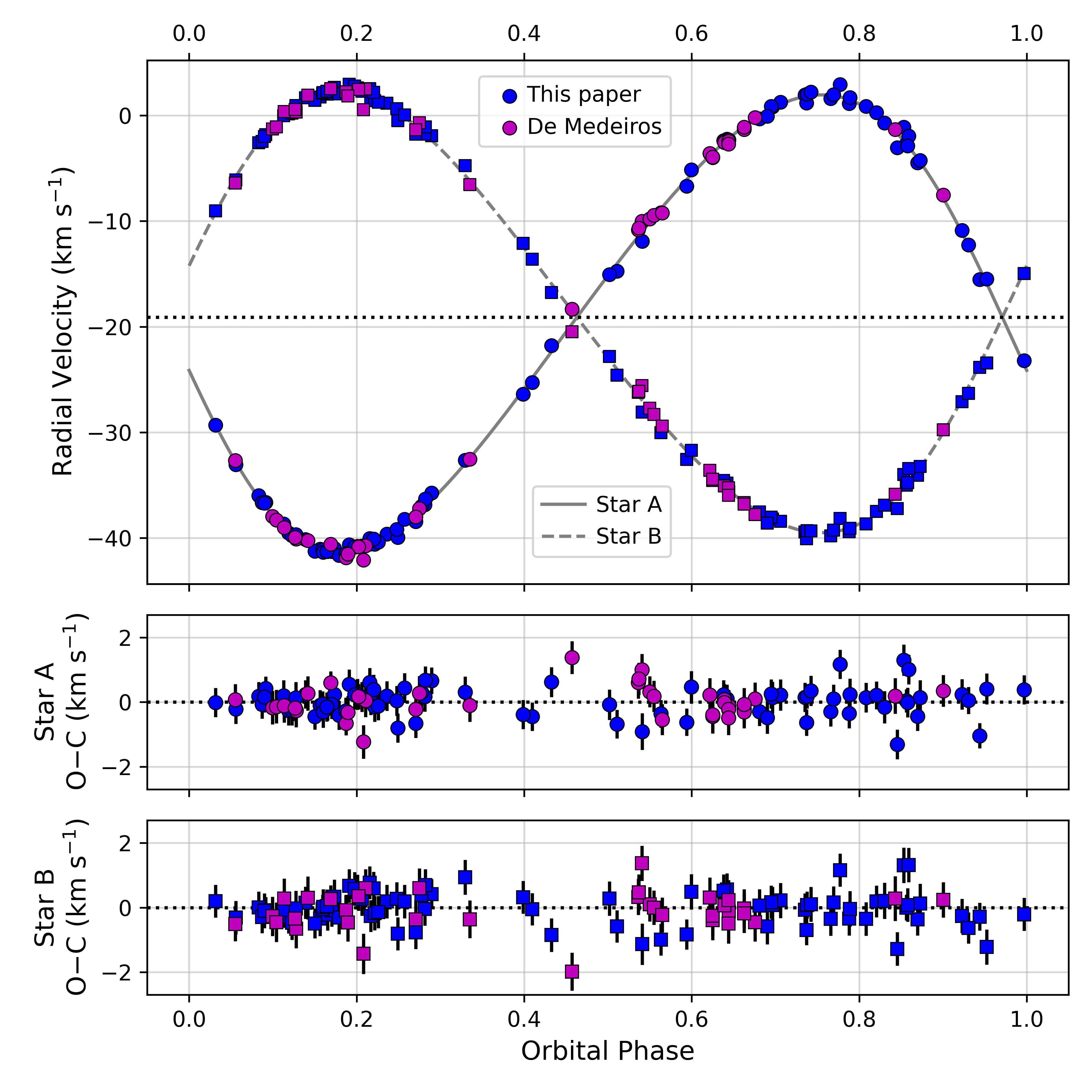
In addition to our own velocities of HD 174881, a data set of similar quality was reported by De Medeiros & Udry (1999), obtained with the CORAVEL spectrometer on the 1m Swiss telescope at the Haute-Provence Observatory (France). Separate spectroscopic orbital solutions with our data and those of De Medeiros give consistent velocity semiamplitudes. We have therefore incorporated the CORAVEL data into our analysis below.
3. Interferometric Observations
3.1. PTI
Near-infrared, long-baseline interferometric measurements of HD 174881 (catalog HD 174881) and calibration sources were conducted with the Palomar Testbed Interferometer (PTI; (Colavita et al., 1999)) in the and bands (m and 2.2 m, respectively) between 2000 and 2006. The maximum PTI baseline (110 m) provided a minimum -band fringe spacing of approximately 4 mas, making the HD 174881 system readily resolvable.
The PTI interferometric observable used for these measurements is the fringe contrast or “visibility” (specifically, the power-normalized visibility modulus squared, or ) of the observed brightness distribution on the sky. HD 174881 was typically observed in conjunction with calibration objects, and each observation (or scan) was approximately 130 seconds long. As in previous publications, PTI data reduction and calibration follow standard procedures described by Colavita et al. (2003) and Boden et al. (1998), respectively. Observations of HD 174881 and associated calibration sources (HD 173667 (catalog HD 173667) and HD 182488 (catalog HD 182488)) resulted in 466 calibrated -band visibility scans on a total of 76 nights spanning a period of nearly 6 years, or about 10 orbital periods.
| JD2,400,000 | Year | Phase | ||||
|---|---|---|---|---|---|---|
| (m) | (m) | (m) | ||||
| 51667.9231 | 2000.3365 | 0.7637 | 2.2225 | |||
| 51667.9254 | 2000.3365 | 0.7641 | 2.2215 | |||
| 51667.9466 | 2000.3366 | 0.7680 | 2.2170 | |||
| 51667.9666 | 2000.3367 | 0.7617 | 2.2246 | |||
| 51677.9241 | 2000.3639 | 0.5891 | 2.2342 |
Note. — Orbital phases were calculated using the ephemeris in Table 6. The values correspond to the effective (flux-weighted) center-band wavelengths of the PTI passband. (This table is available in its entirety in machine-readable form).
3.2. CHARA
The CHARA Array is the world’s longest baseline optical/infrared interferometer, with six 1m telescopes spread across Mt. Wilson, California (ten Brummelaar et al., 2005). The maximum baseline of 330m affords an angular resolution of mas, when observing in the near-infrared band (1.65 m).
HD 174881 was observed in the band on the nights of UT 2007 Jul 04 and UT 2007 Jul 07, with the (then) recently-commissioned Michigan InfraRed Combiner (MIRC; Monnier et al., 2004). At that time, MIRC could combine light from any four CHARA telescopes, measuring six baselines and four closure phases simultaneously. These archival data were processed with an IDL pipeline that used conventional Fourier Transform techniques to extract the visibility and phases from the fringes created in the image plane. The calibrated data were saved in the OI-FITS format (Pauls et al., 2005), and will be deposited with the OI Database hosted at the Jean-Marie Mariotti Center (https://jmmc.fr).
The first night of data (UT 2007 Jul 04) was rather limited, including only three CHARA telescopes (S1-W1-W2) and using the calibrator Lyr (uniform-disk angular diameter mas). The second night (UT 2007 Jul 07) had more and better quality data using four telescopes (S1-E1-W1-W2), with Cyg as the primary calibrator ( mas). Calibrator diameter estimates were based on a combination of an internal MIRC calibrator study (unpublished) and visible-light measurements by the PAVO instrument (Maestro et al., 2013).
Fitting simultaneously for binary separation, flux ratio, and component diameters allowed us to measure the sizes of the individual components of HD 174881. Using only the data from the higher-quality UT 2007 Jul 07 dataset, we measured uniform-disk diameters of mas for star A, mas for star B, and a flux ratio (B/A) of in the band. Table 3 contains the measured separations and position angles between the components from both dates. Note that the component sizes from UT 2007 Jul 07 were used as fixed values for fitting the binary model for UT 2007 Jul 04, as the earlier and smaller dataset could not constrain the sizes on its own.
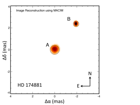
While model fitting is the most reliable and precise way to characterize the MIRC data, we also produced an image reconstruction of HD 174881 using the MACIM algorithm (Ireland et al., 2006). Because of the highly sparse coverage, we used an image prior of two Gaussians (with full width at half maximum of 0.5 mas) centered on the expected locations of the stars based on modeling. We further employed a “uniform disk” regularizer, which is the -norm of the spatial gradient of the image, first described by Baron et al. (2014). Figure 1 shows the MACIM image along with diameter circles from model fitting. The agreement between model and image is excellent. A more detailed comparison between the observations and the model is provided in the Appendix.
| MJD | UT Date | |||||
|---|---|---|---|---|---|---|
| (deg) | (mas) | (mas) | (mas) | (deg) | ||
| 54285.326 | 2007 Jul 04 | 315.1 | 3.09 | 0.216 | 0.04 | 45.1 |
| 54288.250 | 2007 Jul 07 | 320.64 | 3.051 | 0.015 | 0.0149 | 50.64 |
Note. — Columns and represent the major and minor axes of the 1- error ellipse for each measurement, and gives the orientation of the major axis relative to the direction to the north. Position angles are referred to the International Celestial Reference Frame (effectively J2000).
4. Spectral Energy Distribution
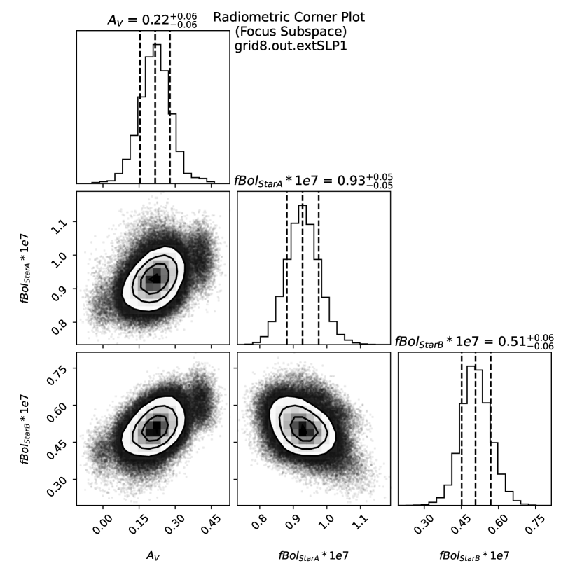
A spectral energy distribution (SED) analysis of the HD 174881 system was used to infer the radiometric parameters (e.g., effective temperature, bolometric flux , and eventually luminosity, when combined with system distance) for each of the components. Flux inputs to the SED modeling presented here are the large collection of archival combined-light photometry and flux measurements available from the literature, in the following photometric systems: Johnson (Mermilliod, 1987), DDO (McClure & Forrester, 1981), Straizys (Straizys et al., 1989), 2MASS (Cutri et al., 2003)111An additional -band measurement was obtained for this work, and is described below in Section 6., AKARI (Murakami et al., 2007), WISE (Cutri et al., 2012), and IRAS (Beichman et al., 1988). Additionally, we used the Gaia BP/RP low-dispersion spectra (Gaia Collaboration et al., 2023), with corrections as recommended by Huang et al. (2024), and importantly also, the in-band component flux ratios. The latter were derived from the system optical spectra at 5187 Å, and the interferometric observables in the and bands from CHARA and PTI, respectively, as described in the preceding sections. These flux and flux ratio data were jointly analyzed with a custom two-component SED modeling code introduced in the work of Boden et al. (2005), using solar metallicity PHOENIX model spectra from Husser et al. (2013). The model atmospheres underlying these spectra adopt spherical geometry for the stellar structure.
Numerical quadratures of the resulting component SED models directly yield estimates for the bolometric fluxes of the individual components. Our modeling suggested that modest extinction along the line of sight is necessary to reproduce the flux set, and this in turn couples into the estimates for component temperatures (through reddening) and bolometric fluxes (which must account for estimated extinction). To robustly estimate component radiometric parameters and uncertainties, we directly evaluated a large grid (roughly cases) spanning the range of viable component temperatures, surface gravities, and system extinction. Those ensemble results were then used to seed Monte Carlo simulations of radiometric parameter a posteriori distributions, and corresponding angular diameter estimates for the stars via , where is the Stefan-Boltzmann constant. Figure 2 illustrates the posterior distributions for the visual extinction and individual component bolometric fluxes, which are the properties showing the strongest correlations.
We note here that our radiometric diameter is not necessarily the same as the wavelength-dependent angular diameters derived interferometrically (even after accounting for limb darkening), such as from MIRC or PTI, although both tell us something about the size of the star. It has been pointed out previously (see, e.g., Mihalas, 1990; Baschek et al., 1991; Scholz, 1997) that the “radius” of a star is not a well defined quantity, as it depends on how it is measured, particularly for giants. In this paper, we follow the practice of other authors (e.g., Hofmann & Scholz, 1998a; Hofmann et al., 1998b; Wittkowski et al., 2004, 2006a, 2006b) and interpret our radiometric angular diameter to be a measure of the size of a star at a Rosseland optical depth of unity. This definition of the radius is commonly used in atmospheric modeling, and in formulating the boundary conditions for interior models.
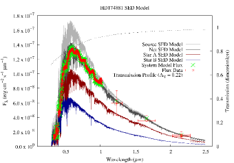
Independent SED-estimated component parameter values for HD 174881 were found to be in good agreement with the spectroscopic analysis from Section 2. Therefore, our preferred a posteriori distributions incorporated Gaussian priors for the component temperatures ( K and K for stars A and B, respectively), as derived in that section. Table 4 summarizes the results, in support of subsequent steps in the analysis of the system. The flux measurements along with our model are presented graphically in Figure 3.
| Parameter | Spectroscopy | SED, no priors | SED, with priors |
|---|---|---|---|
| Star A | |||
| (K) | |||
| (mas) | |||
| ( erg s-1 cm-2) | |||
| (mag) | |||
| Star B | |||
| (K) | |||
| (mas) | |||
| ( erg s-1 cm-2) | |||
| (mag) | |||
Note. — Our adopted SED solution is the one that includes the temperature priors.
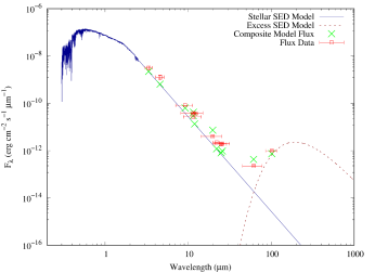
During our SED analysis, it became apparent that archival flux measurements for HD 174881 beyond around 5 m exhibited excess flux relative to photospheric expectations. The situation is depicted in Figure 4, which shows long-wavelength flux measurements plotted against the (sum of Rayleigh-Jeans extensions for) stellar component SEDs. Modest IR excess flux is apparent over most of the range from 5–50 m. Apparent excesses in the IRAS bands at 60 and 100 m are much more dramatic. A simplistic blackbody model fit against these apparent excesses would suggest significant amounts of cool (15–20 K) dust in the HD 174881 system, and this would also seem consistent with the levels of apparent extinction in the radiometric modeling (Table 4). Further investigation of this IR excess will be the topic of ongoing study.
5. Orbital Solution
The PTI observations and radial-velocity measurements from our own observations, as well as those of De Medeiros & Udry (1999), were analyzed together to derive the astrometric and spectroscopic orbital parameters of HD 174881 simultaneously. The usual elements are the orbital period (), a reference time of periastron passage (), the eccentricity () and argument of periastron for star A (), the velocity semiamplitudes (, ), the center-of-mass velocity (), the angular semimajor axis (), the inclination angle (), and the position angle of the ascending node (). The -band flux ratio , which is constrained by the PTI observations, is an additional parameter in this case. The angular diameters of the components also need to be specified (see below). For convenience, the eccentricity and were recast for our analysis as and (see, e.g., Anderson et al., 2011; Eastman et al., 2013), and the inclination angle as . We also allowed for a possible systematic shift () between the De Medeiros & Udry (1999) velocities and our own.
The analysis was carried out in a Markov Chain Monte Carlo framework using the emcee222https://emcee.readthedocs.io/en/stable/index.html package of Foreman-Mackey et al. (2013). We applied uniform priors over suitable ranges for all of the above adjustable parameters. We verified convergence by visual inspection of the chains, and also required a Gelman-Rubin statistic of 1.05 or smaller (Gelman & Rubin, 1992).
To guard against internal observational errors that may be either too small or too large, we included additional free parameters representing multiplicative scaling factors for all uncertainties, separately for the radial velocities of star A and star B from the CfA and from De Medeiros & Udry (1999), as well as for the squared visibilities from the PTI. These scale factors were solved for simultaneously and self-consistently with the other free parameters (see Gregory, 2005), using log-uniform priors.
Estimates of the angular size of star A, from MIRC and Section 4, indicated it may be resolved by the PTI. We therefore added its (uniform disk) angular diameter as a freely adjustable parameter. The other component, on the other hand, is too small to be resolved. Nevertheless, rather than holding the value of fixed, we allowed it to vary within wide ranges, subject to priors based on the results from MIRC and Section 4. The motivation for this is to allow any uncertainty in to propagate through the analysis to all other parameters. The MIRC diameter was measured in the band, rather than , and estimating what it would translate to in would require detailed modeling for HD 174881 to account for differences in opacities and other atmospheric properties at both wavelengths. As we expect the difference to be smaller than the formal uncertainty, here we have simply chosen to use the -band value to establish a Gaussian -band prior from MIRC. And as our wavelength-independent value from Section 4 is not directly related to what is measured by the PTI, in this case we chose to define a loose uniform prior with a conservative 3 half width. Both of these priors were applied simultaneously to determine .
An initial solution for the uniform-disk diameter of star A produced the value mas. This of the same order as our earlier estimates from MIRC ( mas) and from the independent radiometric analysis of Section 4 ( mas). Having verified that there are no serious disagreements, for our final MCMC solution we incorporated the information from latter two measurements by applying priors on in the same way as done above for star B. As the main goal of this analysis was to derive accurate orbital parameters for HD 174881, and are regarded here merely as nuisance parameters. The different estimates of the angular diameters for stars A and B are summarized in Table 5.
| Source | ||
|---|---|---|
| (mas) | (mas) | |
| MIRC ( | ||
| SED Analysis ( | ||
| Initial PTI AnalysisaaThis MCMC analysis imposed simultaneous priors on based on results from MIRC and the SED (see the text), but left completely free. It was meant to verify that the constraint on the diameter of star A from the PTI alone is consistent with the estimates from the two methods above. The exercise proved that to be the case. () | ||
| Final PTI AnalysisbbThese estimates used the same priors on as above, and incorporated the information from MIRC and the SED fit in the form of additional priors on . () |
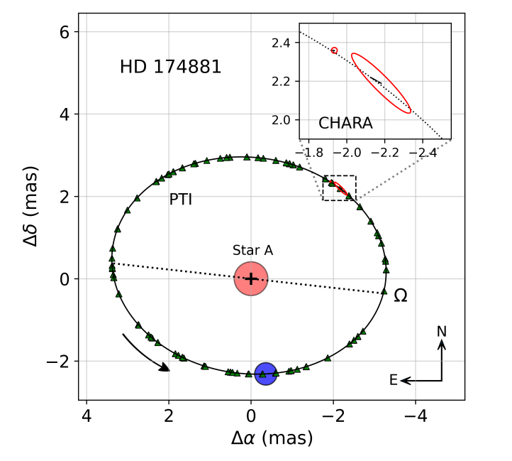
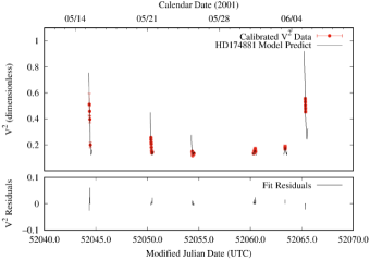
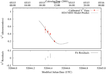
The complete results of our orbital analysis are presented in Table 6. Our astrometric orbit model is shown in Figure 5, in which the PTI measurements, which cannot be represented in this plot, are shown as triangles at their predicted locations. The inset displays the two archival CHARA observations, which were not included in the fit but match the predicted relative positions well within their uncertainties. The radial velocities are shown with the spectroscopic orbit in Figure 6. An illustration of the fit to the PTI visibilities is shown in Figure 7.
| Parameter | Value | Prior |
|---|---|---|
| (day) | [100, 300] | |
| (HJD2,400,000) | [51800, 51900] | |
| [, 1] | ||
| [, 1] | ||
| (mas) | [1, 10] | |
| [, 1] | ||
| (deg) | [0, 360] | |
| (km s-1) | [, 0] | |
| (km s-1) | [10, 50] | |
| (km s-1) | [10, 50] | |
| (km s-1) | [, 5] | |
| [0.1, 3.0] | ||
| (mas) | ||
| (mas) | ||
| , (km s-1) | , 0.50 | [, 5] |
| , (km s-1) | , 0.45 | [, 5] |
| , (km s-1) | , 0.56 | [, 5] |
| , (km s-1) | , 0.47 | [, 5] |
| , | , 0.016 | [, 5] |
| Derived quantities | ||
| (deg) | ||
| (deg) | ||
| Total mass () | ||
| () | ||
| () | ||
| (au) | ||
| (mas) | ||
| Distance (pc) | ||
| () | ||
| () | ||
| (cgs) | ||
| (cgs) | ||
Note. — The values listed correspond to the mode of the posterior distributions, and the uncertainties are the 68.3% credible intervals. and are the scale factors for the internal errors of the CfA RV velocities of the two components. A similar notation is used for the RVs of De Medeiros & Udry (1999), and the PTI. Values following these scale factors on the same line are the weighted rms residuals, after application of the scale factors. Priors in square brackets are uniform over the ranges specified, except for those of the error scaling factors , which are log-uniform. For and , the notation indicates the product of Gaussian and Uniform priors as described in the text. All derived quantities in the bottom section of the table were computed directly from the Markov chains of the fitted parameters involved. The absolute radii depend on the radiometric angular diameters from Section 4, and our distance. With the masses, we then computed .
We note that the position angle of the ascending node (), as determined from the combination of PTI measurements and radial velocities, still suffers from a 180° ambiguity due to the fact that the interferometric squared visibilities are invariant under a point-symmetric inversion around the binary origin. The MIRC observations of HD 174881 break that degeneracy.
The Gaia mission has reported a spectroscopic orbit for HD 174881 (source ID 2040514502502017536) in its most recent data release (DR3; Gaia Collaboration et al., 2023), in which the velocities of both components were measured. The elements are reproduced in Table 7, for easier comparison with the results of this paper. While the Gaia orbit is largely correct, several of the elements show significant deviations from our more precise values.
Our inferred distance for HD 174881, pc, is in excellent agreement with the value derived from the Gaia DR3 parallax, after adjusting it for the zeropoint offset reported by Lindegren et al. (2021). The Gaia value is pc.
| Parameter | Value |
|---|---|
| (days) | |
| (HJD2,400,000)aaThis time of periastron passage is shifted forward by 26 orbital cycles from our value in Table 6. Adjusting it backwards using our more precise period gives 51828.76. | |
| (deg) | |
| (km s-1) | |
| (km s-1) | |
| (km s-1) |
6. Discussion
The main properties of the HD 174881 stars are collected in Table 8. The fainter component (star B) is the more massive one, and is therefore more evolved. It would typically be referred to as the “primary” in the system. It is smaller and hotter than its companion.
| Parameter | Star A | Star B |
|---|---|---|
| () | ||
| () | ||
| (cgs) | ||
| (K) | ||
| Distance (pc) | ||
| (mag) | ||
| (mag) | ||
| (mag) | ||
| (mag) | ||
Note. — The sources of the above properties are as follows: , , , and the distance are taken from Table 6. The temperatures are spectroscopic (Section 2). The luminosities rely on the bolometric fluxes from the radiometric analysis, and the distance. Extinction also comes from the radiometric analysis. The absolute magnitudes depend on the system magnitudes in each bandpass, extinction, the measured flux ratios, and the distance (see the text).
Here we compare these properties against two sets of recent stellar evolution models, under the assumption that the components are coeval. To further constrain the models, we have added to the wavelength-independent dynamical properties and the bolometric luminosities the (extinction-corrected) absolute magnitudes of the components in the , , and bandpasses. They depend on the combined-light brightness, the in-band flux ratios, and our distance estimate. The flux ratio in the band was obtained by applying a small correction to our spectroscopic value reported in Section 2, with the aid of PHOENIX model spectra from Husser et al. (2013) appropriate for the two stars. We obtained (. The values in the near infrared have been reported earlier, and are ( and (, with slightly more conservative uncertainties adopted here than the nominal ones. The apparent magnitude of the system in the visual band was taken to be (Mermilliod, 1987). Due to its near-infrared brightness, HD 174881 is saturated in the 2MASS and bands. For , we had little choice but to adopt the 2MASS value as published (), with its correspondingly large uncertainty. For the band, we were able to gather new measurements with the generous help of our colleague Cullen Blake, on the nights of 2006 November 2 and November 8. These observations were made on the 1.3m PAIRITEL telescope (Blake et al., 2008), located at the Fred L. Whipple Observatory, which was equipped with the same near-infrared camera that was originally used for the southern portion of the 2MASS Survey. The average for the two nights is , which is consistent with, but more precise than, the original 2MASS value of .
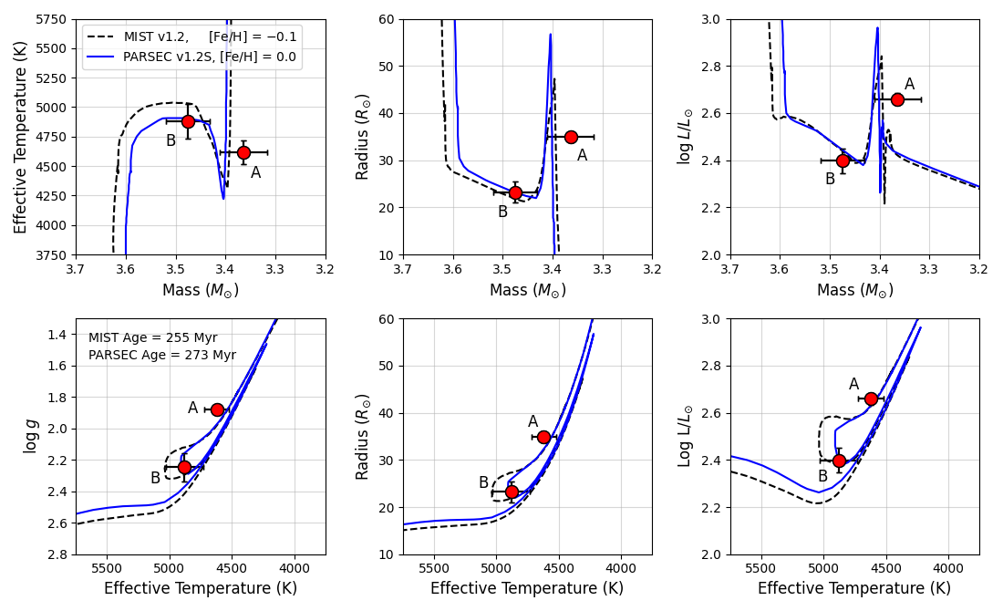
Figure 8 presents the comparison of the HD 174881 properties with isochrones from the MIST v1.2 models of Choi et al. (2016), as well as the PARSEC v1.2S models of Chen et al. (2014). Both sets of models use plane-parallel geometry for the atmospheres at the values of the A and B components, although differences compared to spherical geometry should not be important at these surface gravities. The six panels illustrate the match to the masses, temperatures, radii, surface gravities, and bolometric luminosities. The wavelength-dependent absolute magnitudes (, , ) are shown in Figure 9, as a function of mass and effective temperature. For the MIST models, the best compromise overall was found for a model having a slightly subsolar composition of . The corresponding age of the best fit model is 255 Myr. For PARSEC, a solar composition isochrone produces a better fit than subsolar, although it is somewhat worse than the best MIST match. The age in this case is 273 Myr.
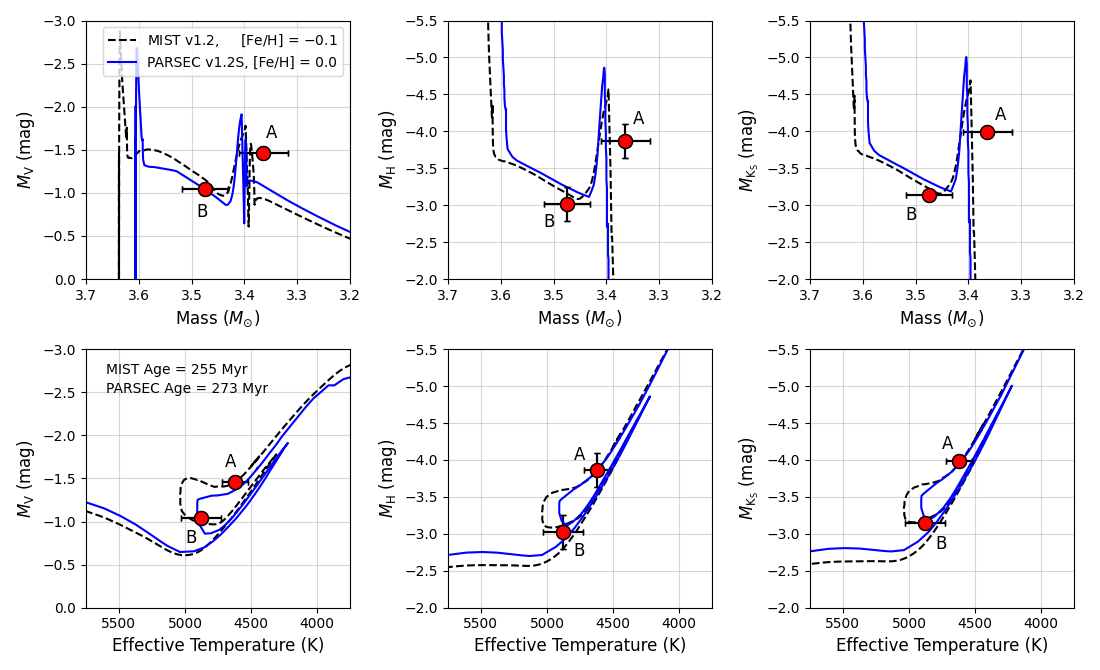
Neither model is able to reproduce all eight measured quantities simultaneously for both stars, within their respective uncertainties. In particular, both isochrones predict that star A (the less massive and therefore less evolved one) should be somewhat cooler and/or less luminous than we observe, if its location is to be consistent with its less evolved state. Indeed, despite these discrepancies, the precision of the observables is such that they easily show the two stars to be in different evolutionary stages. While the more massive component (star B) is clearly located in the helium-burning clump, the location of the other star is either on the first ascent of the giant branch, or on its way down to the clump. The former position appears more likely, based on the sum total of the observations (e.g., top panels of Figures 8 and 9).
The progenitors of both components were late B-type stars. Such objects typically have relatively high initial rotation rates on the zero-age main sequence, which theory shows can affect their observable properties at later stages of evolution (see, e.g., Meynet & Maeder, 1997). An additional comparison (not shown) was made against a version of the MIST isochrones that includes the effects of rotation (, where here is the angular rotation rate, and is the value at breakup). The results are rather similar to the non-rotating case, with the best match to the observations being achieved at a marginally older age of 259 Myr.
7. Conclusions
Precise, model-independent mass determinations for giant stars are still relatively uncommon, compared to similar studies for main-sequence stars. In this paper, we have combined long-baseline interferometry and high-resolution spectroscopy for the giant system HD 174881, to derive absolute masses with precisions of 1.3% for both components, along with a distance (orbital parallax) good to 0.6%. We have also determined the absolute radius of the less massive, larger, and cooler star with an error of just 3.8%, while the size of the other star is less well determined (7.9%). The effective temperatures of both components have been inferred from spectroscopy. Additionally, by incorporating flux measurements in a number of bandpasses, we have derived estimates of the bolometric luminosities as well as the absolute magnitudes in three different bandpasses (, , ), in ways that are not completely dependent on the previously determined properties, thereby adding new information.
In aggregate, these properties provide stringent constraints on models of stellar evolution for evolved stars. Comparisons against two sets of current models (MIST v1.2, PARSEC v1.2S) indicate fair agreement for compositions near solar and ages in the range 255–273 Myr, although discrepancies remain for some of the measured properties. The more massive star resides in the helium-burning clump, while the location in the H–R diagram of the other, less evolved component is still somewhat ambiguous. It is either on the first ascent of the giant branch, or on the subsequent descent toward the clump, the former being favored by the observations.
References
- Andersen (1991a) Andersen, J. 1991a, A&A Rev., 3, 91
- Andersen et al. (1991b) Andersen, J., Clausen, J. V., Nordström, B., Tomkin, J., & Mayor, M. 1991b, A&A, 246, 99
- Andersen (1997) Andersen, J. 1997, in Fundamental Stellar Properties: The Interaction between Observation and Theory, IAU Symp. 189, eds. T. R. Bedding, A. J. Booth & J. Davis (Dordrecht: Reidel), 99
- Andersen (2003) Andersen, J. 2003, in Interferometry for Optical Astronomy II, Proc. SPIE 4838, ed. W. A. Traub, p. 466
- Anderson et al. (2011) Anderson, D. R., Collier Cameron, A., Hellier, C., et al. 2011, ApJ, 726, L19
- Appleton, Eitter & Uecker (1995) Appleton, P. N., Eitter, J. J., & Uecker, C. 1995, J. Astrophys. Astr., 16, 37
- Baron et al. (2014) Baron, F., Monnier, J. D., Kiss, L. L., et al. 2014, ApJ, 785, 46
- Baschek et al. (1991) Baschek, B., Scholz, M., & Wehrse, R. 1991, A&A, 246, 374
- Beichman et al. (1988) Beichman, C. A., Neugebauer, G., Habing, H. J., et al. 1988, Infrared astronomical satellite (IRAS) catalogs and atlases. Volume 1: Explanatory supplement, 1
- Blake et al. (2008) Blake, C. H., Bloom, J. S., Latham, D. W., et al. 2008, PASP, 120, 860
- Boden et al. (2005) Boden, A. F., Torres, G., & Hummel, C. A. 2005, ApJ, 627, 464
- Boden et al. (1998) Boden, A. F., van Belle, G. T., Colavita, M. M., et al. 1998, ApJ, 504, L39
- Chen et al. (2014) Chen, Y., Girardi, L., Bressan, A., et al. 2014, MNRAS, 444, 2525
- Choi et al. (2016) Choi, J., Dotter, A., Conroy, C., et al. 2016, ApJ, 823, 102
- Colavita et al. (1999) Colavita, M. M., Wallace, J. K., Hines, B. E., et al. 1999, ApJ, 510, 505
- Colavita et al. (2003) Colavita, M., Akeson, R., Wizinowich, P., et al. 2003, ApJ, 592, L83
- Cutri et al. (2003) Cutri, R. M., Skrutskie, M. F., van Dyk, S., et al. 2003, The IRSA 2MASS All-Sky Point Source Catalog, NASA/IPAC Infrared Science Archive http://irsa.ipac.caltech.edu/applications/Gator/
- Cutri et al. (2012) Cutri, R. M., Wright, E. L., Conrow, T., et al. 2012, Explanatory Supplement to the WISE All-Sky Data Release Products
- De Medeiros & Udry (1999) De Medeiros, J. R., & Udry, S. 1999, A&A, 346, 532
- Eastman et al. (2013) Eastman, J., Gaudi, B. S., & Agol, E. 2013, PASP, 125, 83
- ESA (1997) ESA 1997, The Hipparcos and Tycho Catalogues, ESA SP-1200
- Foreman-Mackey et al. (2013) Foreman-Mackey, D., Hogg, D. W., Lang, D., & Goodman, J. 2013, PASP, 125, 306
- Gaia Collaboration et al. (2023) Gaia Collaboration, Vallenari, A., Brown, A. G. A., Prusti, T., et al. 2023, A&A, 674, A1
- Gallenne et al. (2016) Gallenne, A., Pietrzyński, G., Graczyk, D., et al. 2016, A&A, 586, A35
- Gelman & Rubin (1992) Gelman, A. & Rubin, D. B. 1992, Statistical Science, 7, 457
- Graczyk et al. (2014) Graczyk, D., Pietrzyński, G., Thompson, I. B., et al. 2014, ApJ, 780, 59
- Graczyk et al. (2018) Graczyk, D., Pietrzyński, G., Thompson, I. B., et al. 2018, ApJ, 860, 1
- Graczyk et al. (2020) Graczyk, D., Pietrzyński, G., Thompson, I. B., et al. 2020, ApJ, 904, 13
- Gregory (2005) Gregory, P. C. 2005, ApJ, 631, 1198
- Hełminiak et al. (2015) Hełminiak, K. G., Graczyk, D., Konacki, M., et al. 2015, MNRAS, 448, 1945
- Hofmann & Scholz (1998a) Hofmann, K.-H. & Scholz, M. 1998a, A&A, 335, 637
- Hofmann et al. (1998b) Hofmann, K.-H., Scholz, M., & Wood, P. R. 1998b, A&A, 339, 846
- Huang et al. (2024) Huang, B., Yuan, H., Xiang, M., et al. 2024, ApJS, 271, 13
- Husser et al. (2013) Husser, T.-O., Wende-von Berg, S., Dreizler, S., et al. 2013, A&A, 553, A6
- Ireland et al. (2006) Ireland, M. J., Monnier, J. D., & Thureau, N. 2006, Proc. SPIE, 6268, 62681T
- Latham (1992) Latham, D. W. 1992, in IAU Coll. 135, Complementary Approaches to Double and Multiple Star Research, ASP Conf. Ser. 32, eds. H. A. McAlister & W. I. Hartkopf (San Francisco: ASP), 110
- Latham et al. (1996) Latham, D. W., Nordström, B., Andersen, J., Torres, G., Stefanik, R. P., Thaller, M., & Bester, M. 1996, A&A, 314, 864
- Latham et al. (2002) Latham, D. W., Stefanik, R. P., Torres, G., Davis, R. J., Mazeh, T., Carney, B. W., Laird, J. B., & Morse, J. A. 2002, AJ, 124, 1144
- Lindegren et al. (2021) Lindegren, L., Bastian, U., Biermann, M., et al. 2021, A&A, 649, A4
- Maestro et al. (2013) Maestro, V., Che, X., Huber, D., et al. 2013, MNRAS, 434, 1321
- McClure & Forrester (1981) McClure, R. D. & Forrester, W. T. 1981, Publications of the Dominion Astrophysical Observatory Victoria, 15, 14
- Mermilliod (1987) Mermilliod, J.-C. 1987, A&AS, 71, 413
- Meynet & Maeder (1997) Meynet, G. & Maeder, A. 1997, A&A, 321, 465
- Mihalas (1990) Mihalas, D. 1990, Astrophysics: Recent Progress and Future Possibilities, eds. B. Gustafsson, & P. E. Nissen (Det Kongelige Danske: Copenhagen), p. 51
- Monnier et al. (2004) Monnier, J. D., Berger, J.-P., Millan-Gabet, R., et al. 2004, Proc. SPIE, 5491, 1370
- Murakami et al. (2007) Murakami, H., Baba, H., Barthel, P., et al. 2007, PASJ, 59, S369
- Nordström et al. (1994) Nordström, B., Latham, D. W., Morse, J. A., Milone, A. A. E., Kurucz, R. L., Andersen, J., & Stefanik, R. P. 1994, A&A, 287, 338
- Pauls et al. (2005) Pauls, T. A., Young, J. S., Cotton, W. D., et al. 2005, PASP, 117, 1255
- Rowan et al. (2024) Rowan, D. M., Stanek, K. Z., Kochanek, C. S., et al. 2024, arXiv:2409.02983
- Scholz (1997) Scholz, M. 1997, IAU Symposium, 189, 51
- Straizys et al. (1989) Straizys, V., Meistas, E., Vansevicius, V., et al. 1989, Vilnius Astronomijos Observatorijos Biuletenis, 83, 3
- ten Brummelaar et al. (2005) ten Brummelaar, T. A., McAlister, H. A., Ridgway, S. T., et al. 2005, ApJ, 628, 453
- Torres et al. (2010) Torres, G., Andersen, J., & Giménez, A. 2010, A&A Rev., 18, 67
- Torres et al. (2000) Torres, G., Andersen, J., Nördstrom, B., & Latham, D. W. 2000, AJ, 119, 1942
- Torres et al. (2009) Torres, G., Claret, A., & Young, P. A. 2009, ApJ, 700, 1349
- Torres et al. (2015) Torres, G., Claret, A., Pavlovski, K., et al. 2015, ApJ, 807, 26
- Torres et al. (1997) Torres, G., Stefanik, R. P., Andersen, J., Nördstrom, B., Latham, D. W., & Clausen, J. V. 1997, AJ, 114, 2764
- Weber & Strassmeier (2011) Weber, M. & Strassmeier, K. G. 2011, A&A, 531, A89
- Wittkowski et al. (2004) Wittkowski, M., Aufdenberg, J. P., & Kervella, P. 2004, A&A, 413, 711
- Wittkowski et al. (2006b) Wittkowski, M., Aufdenberg, J. P., Driebe, T., et al. 2006b, A&A, 460, 855
- Wittkowski et al. (2006a) Wittkowski, M., Hummel, C. A., Aufdenberg, J. P., et al. 2006a, A&A, 460, 843
- Zucker & Mazeh (1994) Zucker, S., & Mazeh, T. 1994, ApJ, 420, 806
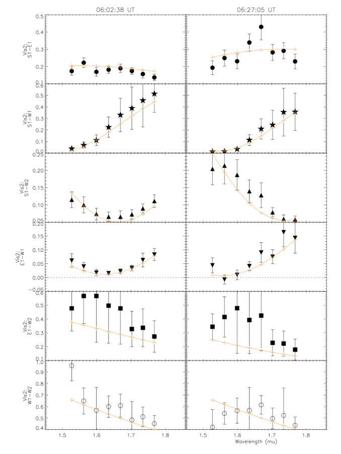
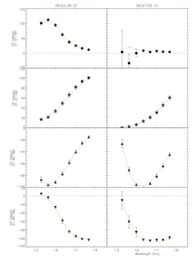
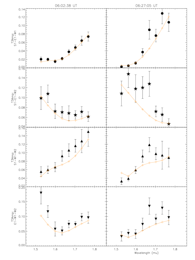
8. Appendix: Comparison of our 2007 July 7 MIRC data and the MACIM image model
The figures in this Appendix compare our MIRC squared visibilities, closure phases, and triple amplitude measurements from the 2007 July 7 observation with the model for the image of HD 174881 displayed in Figure 1. The reduced values we obtained from the fit are 0.753 for the visibilities, 0.406 for the closure phases, and 1.571 for the triple amplitudes.