Wavelength modulation laser spectroscopy of N₂O at 17 µm

Abstract

Using a mid-infrared quantum cascade laser and wavelength modulation absorption spectroscopy, we measure the frequencies of ro-vibrational transitions of N₂O in the 17 $\mu$m region with uncertainties below 5 MHz. These lines, corresponding to the bending mode of the molecule, can be used for calibration of spectrometers in this spectral region. We present a model for the lineshapes of absorption features in wavelength modulation spectroscopy that takes into account Doppler broadening, collisional broadening, saturation of the absorption, and lineshape distortion due to frequency and intensity modulation. Combining our data with previous measurements, we provide a set of spectroscopic parameters for several vibrational states of N₂O. The lines measured here fall in the same spectral region as a mid-infrared frequency reference that we are currently developing using trapped, ultracold molecules. With such a frequency reference, the spectroscopic methods demonstrated here have the potential to improve frequency calibration in this part of the spectrum.

1 Introduction

The mid-infrared is an important spectral region with applications in trace gas detection [1, 2, 3], atmospheric monitoring [4, 5], high resolution spectroscopy [6, 7, 8, 9], frequency metrology [10, 11, 12, 13, 14], measurements of fundamental constants [15] and tests of fundamental physics [16, 17, 18]. The wavelength region between 7 and 20 $\mu$m is known as the molecular fingerprint region, because every molecule has a unique spectrum in this region. However, the spectroscopic potential of this region has been difficult to exploit because (i) spectra are often crowded, requiring high resolution, (ii) laser technology in many parts of this region is often poorly developed or non-existent, (iii) optical elements often absorb strongly, especially beyond 15 $\mu$m, (iv) there are not many absolute frequency standards in this spectral region, and (v) calibration of the frequency axis is difficult. A new generation of quantum cascade lasers at wavelengths beyond 10 $\mu$m is helping to solve some of these problems, see e.g. [19]. Here, we use a quantum cascade laser to demonstrate laser spectroscopy at 17 $\mu$m with an accuracy of a few MHz.

Nitrous oxide, N₂O, is a common gas that is often used for frequency calibration in the mid-infrared [20]. Environmental monitoring of this gas is important since it is the dominant anthropogenic cause of ozone depletion and is a potent greenhouse gas whose atmospheric concentration has been rising for decades [21]. The fundamental vibrational frequency of the bending ($\nu_{2}$) mode of N₂O lies near 17 $\mu$m, and the gas has a forest of strong absorption lines in this spectral region.

There exist two large spectroscopic databases providing comprehensive line lists for N₂O throughout the mid-infrared. The first is the HITRAN database [22] which gives a line list for N₂O based in part on the data provided by Toth [23], which is calculated from spectroscopic constants derived from measurements by the same author. The second, which we call the NIST database, is described in Ref. [20] and supported by line lists provided in tabular form and online [24]. The line list is built from spectroscopic constants derived from a wide range of data sources including microwave spectroscopy, Fourier transform spectroscopy and heterodyne frequency measurements. The heterodyne measurements are described in [25] and a series of papers from NIST that include Refs. [26, 27, 28, 29, 30]. They provide absolute frequencies for a selection of lines which are denoted as recommended calibration lines in the NIST database. In the region around 17 $\mu$m, the accuracy of these calibration lines reaches 3 MHz. We note that the frequencies of lines in the $\nu_{2}$ bands were not measured directly, but instead derived through a combination of frequency measurements of other bands at shorter wavelengths, e.g. [30].

There has been very little prior laser spectroscopy of the $\nu_{2}$ band of N₂O. In earlier work [31, 32, 33] using a lead salt laser, a set of lines were measured with a relative precision of 30 MHz. Recently, a quantum cascade laser (QCL) operating at 17.2 $\mu$m was developed and its spectral properties were measured using absorption lines of N₂O [34]. In this paper, we demonstrate wavelength modulation spectroscopy of N₂O using this QCL. We measure 165 lines in the small region between 580.3 and 582.5 cm^-1 and determine their frequencies. Because the method has high sensitivity and high dynamic range, we are able to observe lines from five different isotopologues and 12 different vibrational bands.

At present, the Bureau International des Poids et Mesures recommends only two frequency standards in the mid-infrared, one at 3.39 $\mu$m based on CH₄ with a relative uncertainty of $3\times 10^{-12}$, and the other at 10.3 $\mu$m based on OsO₄ with an uncertainty of $1.4\times 10^{-13}$ [35]. Recent advances in cooling and controlling neutral molecules [36, 37] and molecular ions [38] raise the prospect of a set of new frequency standards in the mid-infrared, based on the vibrational frequencies of trapped molecules, whose precision could match that available in the microwave and optical domains ($10^{-16}$ or better). These frequency standards could then be used to calibrate large sets of spectral lines in common gases such as N₂O. Suitable molecular clocks are currently being developed, motivated in part by their potential to search for varying fundamental constants [39, 18, 40, 41, 42]. The QCL used in the present work has been designed so that its frequency coincides with the fundamental vibrational frequency of CaF molecules, which can be cooled to microkelvin temperature [43] and can make an outstanding frequency standard [18]. We consider the prospects of improving frequency calibration in this spectral region through the combination of an absolute frequency reference provided by CaF molecules, the set of strong and narrow absorption lines provided by N₂O and other gases, and the reliable source of laser light provided by QCL technology.

2 Methods

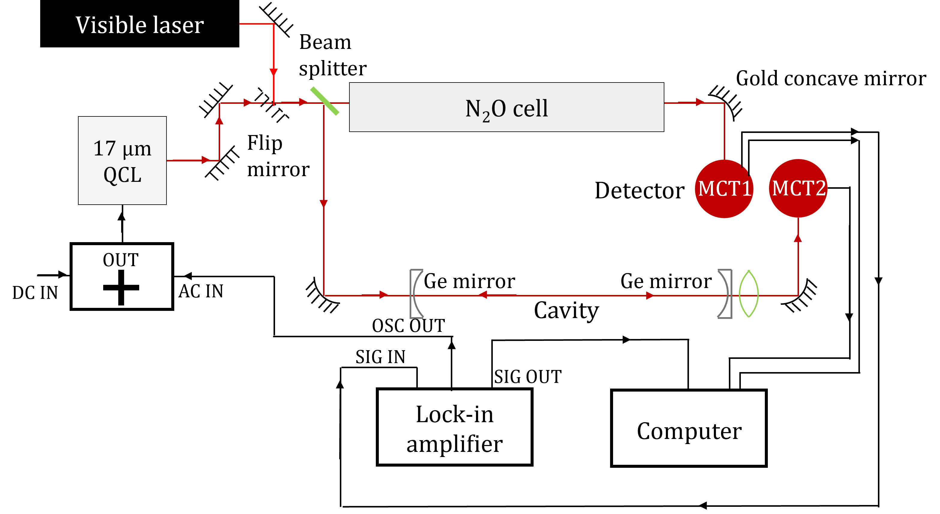
Figure 1: Schematic of the experimental setup. The 17 $\mu$m laser beam is divided into two parts, one passing through the N₂O cell for absorption spectroscopy, and the other through a cavity for frequency calibration. A visible laser is used as an alignment aid. The laser frequency is modulated and the absorption signal at a harmonic of the modulation frequency is detected using a lock-in amplifier. OSC OUT is the modulation fed to the laser; SIG IN is the direct absortion signal; SIG OUT is the output of the lock-in amplifier.

Figure 1 illustrates the experimental setup we use for wavelength modulation spectroscopy. The light from the QCL is separated into two beams, each with a power of approximately 0.5 mW. The first beam, used for absorption spectroscopy, passes through a gas cell of length 20 cm containing about 350 Pa of N₂O, and then onto a liquid nitrogen cooled mercury cadmium telluride detector, MCT1, that measures its power. By applying an oscillating component to the current of the QCL, its frequency is modulated with $f_{\rm mod}=2.22$ kHz and a modulation amplitude of roughly 20 MHz. This modulation amplitude is not small compared to the typical N₂O linewidths (FWHM) of about 36 MHz, so we include the effects of the modulation in the lineshape model discussed later and in A. A lock-in amplifier detects the amplitude of the oscillating signal at MCT1 at either $f_{\rm mod}$ or $2f_{\rm mod}$. The second beam, used to calibrate the frequency scale, passes through a confocal cavity and then onto a separate detector, MCT2. The cavity is formed from a pair of plano-concave lenses separated by 30 cm and made from germanium whose refractive index at 17.2 $\mu$m is $n=3.9997$, giving a reflectivity of 35.9%. The cavity provides a set of frequency markers with a spacing of $\delta f=c/(4L)\approx 250$ MHz. The signals from MCT1, MCT2 and the lock-in amplifier are recorded simultaneously. The placements of all optical components are carefully adjusted to minimize etaloning effects from back reflections.

3 Results and analysis

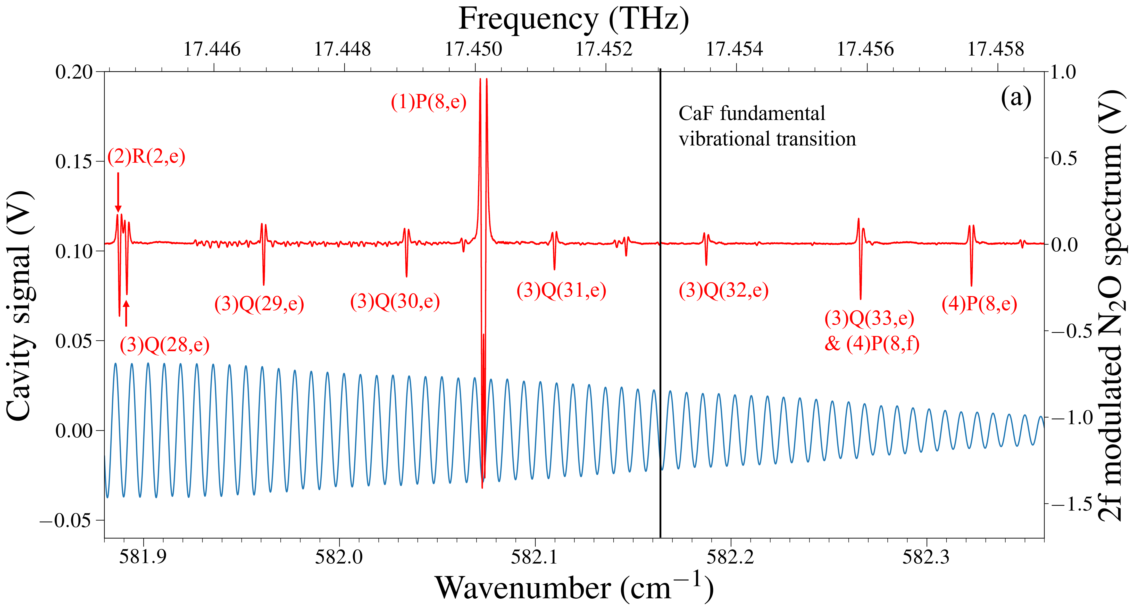
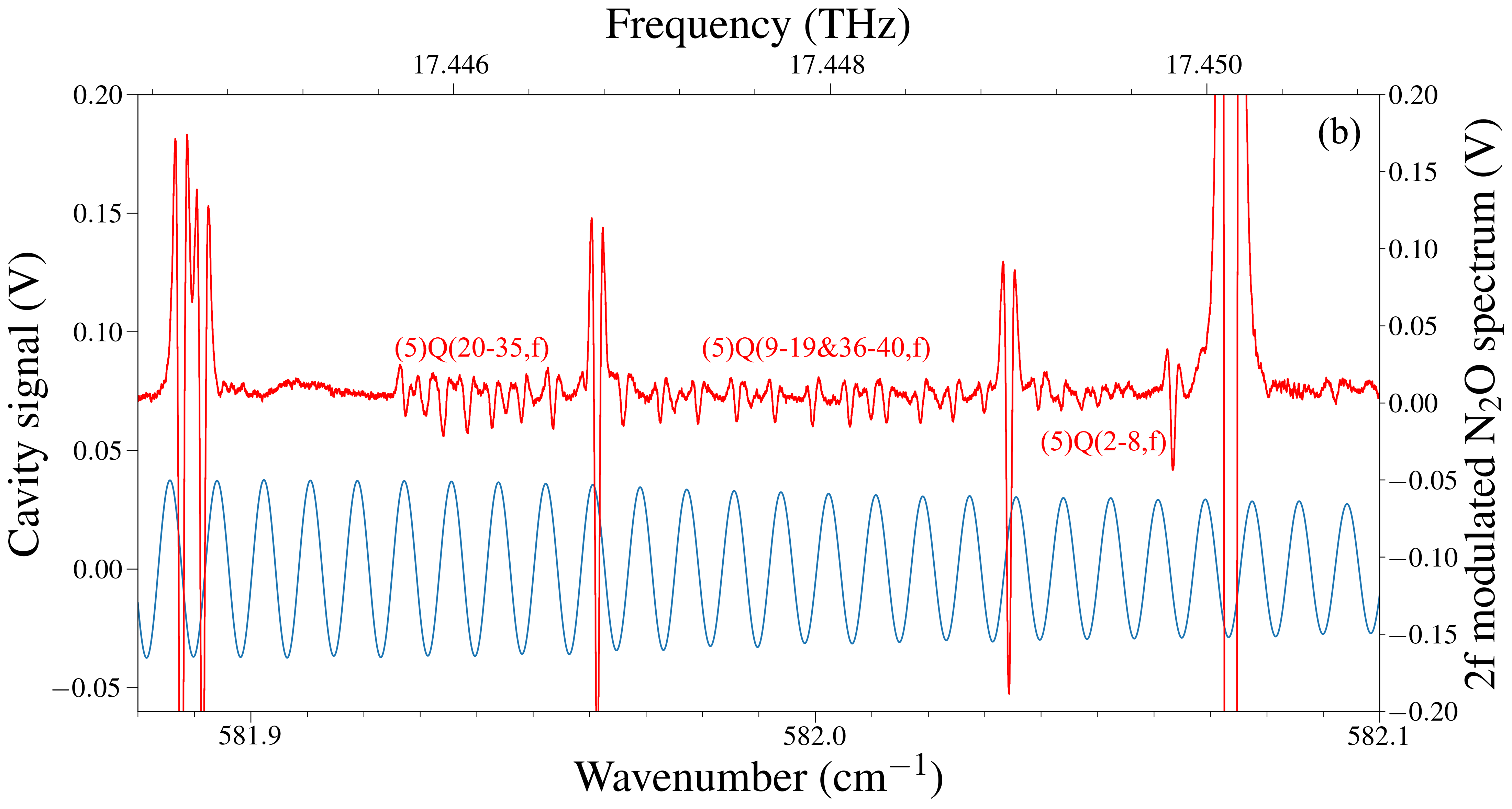
Figure 2: Examples of measured ¹⁴N${}_{2}^{16}$O rovibrational transitions detected at $2f_{\rm mod}$ (red), together with cavity fringes (blue). (a) Part of spectrum spanning 0.48 cm^-1. Vertical black line indicates the frequency of the CaF $v^{\prime}=1\leftarrow v=0$ P(1) transition [44, 45] (b) Expanded region spanning 0.22 cm^-1, showing many smaller lines. Transitions are labelled in the format ‘(band)P/Q/R(J,e/f)’ with vibrational bands denoted: (1): $(01^{1}0)-(000)$; (2): $(02^{0}0)-(01^{1}0)$; (3): $(03^{1}0)-(02^{0}0)$; (4): $(02^{2}0)-(01^{1}0)$ (5): $(04^{2}0)-(03^{1}0)$.

N₂O is a linear triatomic molecule with a ${}^{1}\Sigma$ ground state. Vibrational states are labelled as $(\nu_{1}\,\nu_{2}^{l}\,\nu_{3})$ where $\nu_{1,2,3}$ are the quantum numbers of the symmetric stretch mode, the bending mode and the antisymmetric stretch mode respectively, and $l$ is the angular momentum associated with the bending mode. The labels $e$ and $f$ are used to denote the symmetry of the $l$-type doubling components following the standard convention [46]. Rotational transitions that have $J^{\prime}=J-1$, $J^{\prime}=J$ and $J^{\prime}=J+1$ are denoted as $P(J)$, $Q(J)$ and $R(J)$ respectively, where $J$ and $J^{\prime}$ are the rotational angular momentum quantum numbers of the lower and upper levels. We focus on a region of the spectrum centred at 581.5 cm^-1 containing strong P lines of the $(01^{1}0)-(00^{0}0)$ band, weaker P lines of the $(02^{2}0)-(01^{1}0)$ band and Q lines of the $(03^{1}0)-(02^{0}0)$ band, and even weaker lines from several other bands. In total, we measure lines in the following 12 bands: $(01^{1}0)-(00^{0}0)$, $(02^{0}0)-(01^{1}0)$, $(02^{2}0)-(01^{1}0)$, $(03^{1}0)-(02^{0}0)$, $(03^{1}0)-(02^{2}0)$, $(03^{3}0)-(02^{2}0)$, $(04^{0}0)-(03^{1}0)$, $(04^{2}0)-(03^{1}0)$, $(04^{2}0)-(03^{3}0)$, $(11^{1}0)-(10^{0}0)$, $(12^{0}0)-(11^{1}0)$, $(12^{2}0)-(11^{1}0)$.

3.1 Example data

Figure 2 shows examples of the data obtained. The red line is the N₂O absorption signal at $2f_{\rm mod}$ and the blue line is the cavity transmission. The laser frequency is scanned at a rate of approximately 180 MHz s^-1 and the data presented are single scans. The frequency is controlled via the QCL current which also changes the power of the laser. That change is reflected in the amplitude of the cavity fringes as the laser is scanned, and its effect is included in our lineshape model (see A). The frequency-dependence of the power is very close to linear so has little effect on the signal at $2f_{\rm mod}$.

Figure 2(a) shows a region of the spectrum spanning 0.48 cm^-1. The strongest line is the P(8) line of the $(01^{1}0)-(00^{0}0)$ band of ¹⁴N${}_{2}^{16}$O. This is listed in the NIST database of recommended calibration lines and is one of the calibration lines used in this work. The other strong lines observed are mainly Q lines of the $(03^{1}0)-(02^{0}0)$ band in this isotopologue. Figure 2(b) is an expanded view of the small region between 581.88 cm^-1 and 582.09 cm^-1 where we see a dense spectrum of much weaker features which are Q lines in the $(04^{2}0)-(03^{1}0)$ band of ¹⁴N${}_{2}^{16}$O. The signal-to-noise ratio for these weak features remains high. Indeed, we observe lines with strengths spanning 4 orders of magnitude (see below).

3.2 Fitting to a model

To fit to these data, we develop a model to describe the lineshapes. This model extends previous work [47, 48] and accounts for Doppler broadening, collisional broadening, the effect of the modulation, saturation of the absorption at large optical depths, and effects due to the frequency dependence of the laser intensity. The model is important for determining accurate frequencies so we describe it in detail in the appendix and more briefly here.

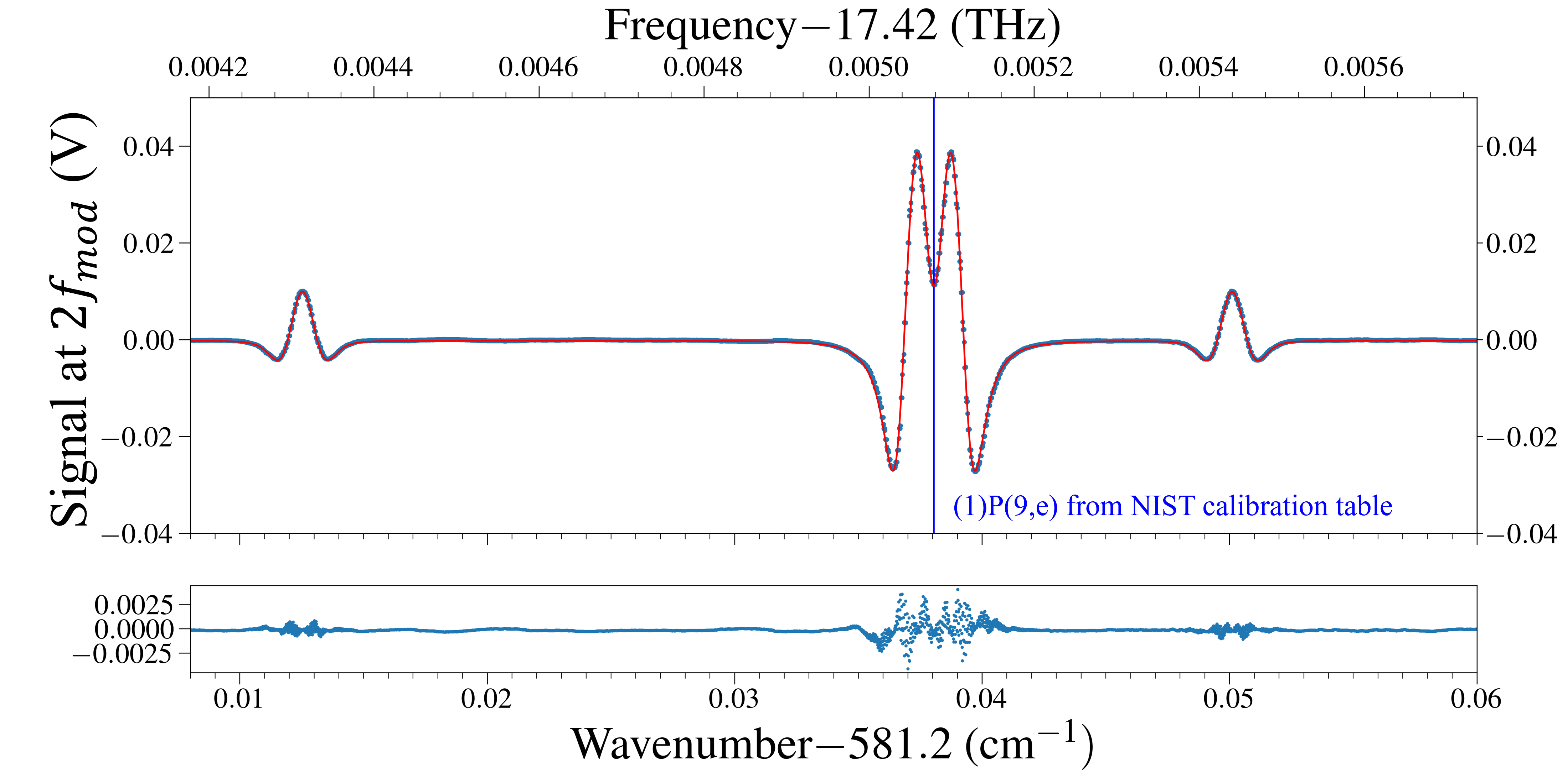
Figure 3: An example fit. Blue dots: absorption signal detected at $2f_{\rm mod}$; Red line: fit to model described by Eqs. (1) and (2). Blue vertical line: (1)P(9,e) transition of ¹⁴N${}_{2}^{16}$O used as a calibration line in this work. The bottom panel shows the fit residuals. Band labelling is the same as in figure 2.

The current of the QCL is modulated with angular frequency $\Omega$, and this modulates both the frequency and intensity of the light. The detuning of the light from the centre of an absorption feature, normalized to the linewidth of the absorption feature, is denoted by $\Delta$. It has two parts, $\Delta=\delta-\delta_{\rm m}\cos(\Omega t)$, where $\delta$ is the detuning averaged over a modulation cycle and $\delta_{\rm m}$ is the modulation amplitude, both normalized to the linewidth. The laser intensity incident on the absorbing sample is $I_{\rm in}=I_{0}(1+p\Delta)$ where $I_{0}$ is the intensity at the centre of the absorption feature and we are assuming a linear dependence on $\Delta$ with proportionality constant $p$. We measure the intensity transmitted through the absorbing sample $I_{\rm out}$ and pick out the component of this signal oscillating at frequency $n\Omega$. As shown in the appendix, this component is

$$\frac{I_{{\rm out},n}}{I_{0}}=2\epsilon_{n}(-1)^{n}\int_{-\delta_{\rm m}}^{\delta_{\rm m}}\frac{\cos\left(n\cos^{-1}\left(\frac{\delta^{\prime}}{\delta_{\rm m}}\right)\right)}{\sqrt{\delta_{\rm m}^{2}-\delta^{\prime 2}}}(1+p\delta-p\delta^{\prime})e^{-\alpha(\delta-\delta^{\prime})}d\delta^{\prime},$$ (1)

where $\epsilon_{0}=1$ and $\epsilon_{n}=2$ for all $n>0$. The function $\alpha(\delta)$ is the optical depth and describes the frequency dependence of the absorption. In the present work, both Doppler broadening and collisional broadening are important, so we choose $\alpha(\delta)$ to be a Voigt profile,

$$\alpha(\delta)=\int_{-\infty}^{\infty}G(\delta^{\prime\prime},\sigma_{1})L(\delta-\delta^{\prime\prime},\sigma_{2})d\delta^{\prime\prime}.$$ (2)

Here $G(\delta,\sigma_{1})$ is a Gaussian function with width parameter $\sigma_{1}$ and $L(\delta,\sigma_{2})$ is a Lorentzian function with width parameter $\sigma_{2}$. In cases where there are several lines close together, we choose $\alpha(\delta)$ to be a sum of Voigt profiles.

Figure 3 shows a small region of the spectrum around 581.2 cm^-1. The points are the data, and the line is a fit to the model described by Eqs. (1) and (2). The free parameters in the fit are the line centre, the peak optical depth and the Gaussian and Lorentzian widths. The value of $p$ is determined independently from the sloping background of the raw absorption data and is fixed in the fit. The parameter $\delta_{\rm m}$ is found for each segment of data from a fit to one of the strong lines, and is then fixed at this value for all the other lines. We also fix $n=2$ since these data are the signals at twice the modulation frequency. We see three lines in Fig. 3. The two smaller ones have low optical depth and their profiles are similar to the second derivative of the Voigt profile. The larger one has high optical depth resulting in saturation of the absorption. This broadens the profile and introduces an extra dip at the centre of the profile which corresponds to the flat top of the saturated absorption line where the second derivative tends towards zero. This central dip becomes deeper and broader as the optical depth increases. Looking at many lines, we find that the fits give large variations for the individual Gaussian and Lorentzian widths, but a consistent value for their quadrature. The mean value is a full width at half maximum (FWHM) of 36 MHz. If we instead fix the FWHM of the Gaussian profile to 31.8 MHz, which is the expected value due to Doppler broadening, the typical Lorentzian width is 12 MHz. This is close to the expected FWHM due to pressure broadening alone, which is 10.5 MHz, where we have used a typical value given by HITRAN [22] for the self-broadening coefficient of these lines, 3 GHz/atm. The high signal-to-noise ratio and the accurate modelling of the line profile allows us to find relative line centres with fitting uncertainties below $10^{-4}$ cm^-1 for almost all lines.

3.3 Data reduction

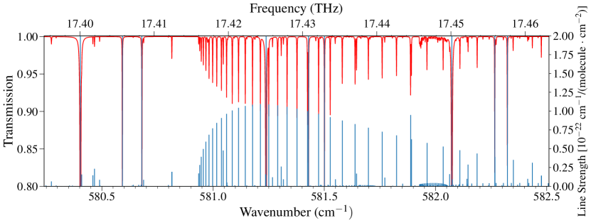
Figure 4: Comparison between our measured N₂O transitions and those in the HITRAN [22] database. The red line is the fitted absorption spectrum converted from the original wavelength modulated spectrum. For this dataset, the left hand axis gives the fraction of incident power transmitted through the cell. The blue sticks are the N₂O transitions from HITRAN [22] and are associated with the line strength given on the right axis. The strongest $\nu_{2}$ lines are much stronger than the other lines, having a height about 35 times the vertical scale of this figure.

We have observed 165 N₂O lines in the frequency range from 580.40 to 582.48 cm^-1. Figure 4 shows the complete spectrum, where we have converted from the 2f modulation data back to the original absorption spectrum using the fitted Voigt parameters. Several strong lines, where the direct absorption is easily measured alongside the 2f data, are used to convert the amplitudes of the lines to the absolute transmission, thereby calibrating the vertical axis. We calibrate the frequency axis using the cavity data and three calibration lines from the NIST database [24], namely the P(8), P(9) and P(10) lines of the $(01^{1}0)-(000)$ band of ¹⁴N${}_{2}^{16}$O. The cavity data determines the frequency scale between each of the calibration lines. To treat the cavity data, we first remove the change in amplitude of the cavity fringes across the scans by normalizing the cavity data to the laser power. The power is determined from the baseline of the raw N₂O absorption spectrum. The resulting cavity fringes are almost sinusoidal because the cavity has such a low finesse. We apply a low-pass filter to the cavity data to remove higher order components, and then fit a sinusoidal model to segments of the data. These segments typically contain 2-7 cavity fringes and are short enough that non-linearity in the conversion from QCL current to frequency is negligible. After piecing the segments together, a cavity phase can be assigned to every point in the scan. The phase difference between two calibration lines, whose frequencies are known, provides the conversion from phase to frequency. In this way, the frequency of every line in the spectrum is determined. The full list of measured frequencies is given in the second column of Tab. LABEL:tab:n2odata.

Next we consider the uncertainties in determining the centre frequencies of all the lines. As detailed in B, there are four main sources of statistical uncertainty. The first comes from the calibration lines which each have a $1\sigma$ uncertainty of 1.5 MHz. The second comes from the fits to the spectral lines. This uncertainty varies enormously between the weak and strong lines. It is about 2 MHz for the weakest lines that we have measured, and about 100 times smaller than this for the strongest lines. The third uncertainty comes from fitting to the cavity data and determining the cavity phase at each of the calibration lines and each of the lines of interest. This varies across the spectrum but is at most 0.4 MHz. The last source of uncertainty is due to the frequency drift of the cavity resulting from drifts of the laboratory temperature and pressure. We monitored these drifts by repeatedly scanning the same frequency region and measuring how the phase of the cavity changes with respect to an N₂O line over time. We also passed a 780 nm laser through the cavity and monitored how the cavity frequency changed relative to an atomic reference (a saturated absorption feature in Rb). The latter is more sensitive because of the shorter wavelength. During an hour-long period of monitoring, we measured a linear cavity drift of 30 kHz/s at 17 $\mu$m. The uncertainty in the spectral line frequencies due to such a linear drift is tiny because the calibration procedure almost perfectly eliminates the effect of the drift when both the drift and the frequency scan are linear in time. To produce a significant effect, the cavity length would need to change suddenly during the scan, or drift in one direction for part of the scan, and then the other direction for the rest. While monitoring the cavity, we did observe occasional sudden (few second) step-like changes in the cavity frequency with amplitudes of about 5 MHz at 17 $\mu$m. We suppose that such changes may have been occurring while acquiring the N₂O data and include the effect as an uncertainty. The uncertainty is largest for spectral lines that are far from a calibration line where they reach about 2.5 MHz. We note that, in most cases, the largest source of uncertainty comes from the calibration lines. This observation suggests that a more accurate absolute reference will be useful in improving the accuracy of all the lines reported here to the sub-MHz level.

Collisions induce both a broadening and a shift of the spectral lines. To estimate this pressure shift, we note that HITRAN gives shift coefficients in air ranging from $-15$ to $+3$ MHz/atm for all lines in this region, while Toth [49] gives an average self-shift coefficient of $-45$ MHz/atm for lines in the region 1800–2630 cm^-1. We did not find a value for the self-shift coefficients for our spectral region, but it should be similar to these values which give a negligible line shift for our operating pressure. We add all uncertainties in quadrature to obtain the total uncertainty on each line. These are given in parentheses in the second column of Tab. LABEL:tab:n2odata, where the number indicates the $2\sigma$ uncertainty in the last digits. For most lines, this is between 3 and 5 MHz. The root mean square (rms) value of the set of uncertainties is 3.6 MHz.

The absolute pressure of N₂O was not calibrated in the present work, so we are not currently able to report spectral line intensities on an absolute scale. Instead, Tab. LABEL:tab:n2odata (last column) gives the relative amplitude of each line in the spectrum which is the fitted value of the amplitude parameter of the Voigt function.

3.4 Comparison with other data

Figure 4, compares our measured spectrum to a model spectrum derived from the HITRAN database [22]. The strengths of these lines span 4 orders of magnitude, and we have chosen a vertical scale where the weakest lines are just visible; the line strengths of the most intense lines are about 35 times larger than the scale of the graph. The measured spectrum is in good agreement with HITRAN for both the frequencies and line strengths. Table LABEL:tab:n2odata lists the frequencies, isotopologues and quantum numbers of all the lines measured in this work and compares our measured frequencies to the ones given in the HITRAN database and the NIST table of calibration lines. Our measurements agree with the values given in HITRAN to better than $6\times 10^{-4}$ cm^-1 (18 MHz) for 148 of the 165 lines, and the rms deviation between HITRAN and our measurements is $4.7\times 10^{-4}$ cm^-1 (14 MHz).

3.5 Molecular parameters

In the literature, three different approaches have been used to model the rotational structure of the vibrational bands of N₂O. They differ in the way they treat the splitting of states with $l\neq 0$ into e and f levels, which we call the $l$-doubling. In the first approach the e and f states are treated as separate vibrational states, each with their own term energy and set of rotational constants. This tends to introduce more parameters than are required. The second method, used for example in [50], describes the energy using the empirical formula

$$E_{v} =G_{v}+B_{v}J(J+1)-D_{v}(J(J+1)-l^{2})^{2}+H_{v}(J(J+1)-l^{2})^{3}$$

$$\pm\frac{1}{2}q_{v}J(J+1)\mp\frac{1}{2}q_{vJ}J^{2}(J+1)^{2}\pm\frac{1}{2}q_{vJJ}J^{3}(J+1)^{3}.$$ (3)

Here, the subscript $v$ stands for the set of quantum numbers $\nu_{1},\nu_{2},l,\nu_{3}$, $G_{v}$ is the term energy, $B_{v}$, $D_{v}$ and $H_{v}$ are rotational constants and $q_{v}$, $q_{vJ}$ and $q_{vJJ}$ are $l$-doubling constants (set to zero when $l=0$). The third approach, used in [20], includes matrix elements of the $l$-doubling Hamiltonian that couples states differing in $l$ by 2 units. This is more consistent, but has the disadvantage that the energies of levels in one vibrational state depend on the parameters of a different vibratonal state. We choose to use the second method and fit to our data using Eq. (3).

We analyze those lines arising from the main isotopologue, ¹⁴N${}_{2}^{16}$O. There is insufficient data for the other isotopologues. For most of the vibrational states in our analysis, the rotational and $l$-doubling parameters have been established to high precision through microwave spectroscopy. The parameters are summarized in Table 1 of [50]. For the states $(00^{0}0)$, $(01^{1}0)$, $(02^{0}0)$, $(02^{2}0)$, $(03^{1}0)$, $(03^{3}0)$, $(11^{1}0)$ and $(10^{0}0)$, we fix $B_{v}$, $D_{v}$, $H_{v}$, $q_{v}$, $q_{vJ}$ and $q_{vJJ}$ to the values given in [50], leaving only the $G_{v}$ as free parameters. The rotational and $l$-doubling parameters for $(04^{2}0)$ and $(12^{0}0)$ are not provided in [50] so we leave them all as free parameters in our fits and determine them from our own data. We fit each band separately to Eq. (3). The output from these fits are the values of the band centre frequencies $\nu_{0}=G_{v^{\prime}}-G_{v}$, together with the rotational and $l$-doubling parameters for $(04^{2}0)$ and $(12^{0}0)$.

Band	$v_{0}$ (cm-1)	Lines	$\chi_{\rm r}^{2}$
$(01^{1}0)-(00^{0}0)$	588.76773(6)	3	$1.5\times 10^{-4}$
$(02^{0}0)-(01^{1}0)$	579.36440(6)	2	20
$(02^{2}0)-(01^{1}0)$	588.97656(6)	6	5.4
$(03^{1}0)-(02^{0}0)$	580.93263(5)	35	3.2
$(03^{3}0)-(02^{2}0)$	589.16739(6)	6	11.9
$(03^{1}0)-(02^{2}0)$	571.32052(5)	6	5.9
$(04^{2}0)-(03^{1}0)$	582.05610(5)	51	2.9
$(11^{1}0)-(10^{0}0)$	595.36234(6)	3	1.5
$(12^{0}0)-(11^{1}0)$	581.73044(7)	21	0.72

Table 1: Band centre frequencies, in cm^-1, for nine vibrational bands of ¹⁴N${}_{2}^{16}$O. The number in the parenthesis is the 1$\sigma$ uncertainty in the last digits. The table also gives the number of lines used in the fit, and the reduced chi-squared.

Table 1 lists the values of $\nu_{0}$ determined from the fits for nine vibrational bands of ¹⁴N${}_{2}^{16}$O, along with their uncertainties. The table also gives the values of the reduced chi-squared, $\chi_{\rm r}^{2}$, which is the sum of the squared standardized residuals divided by the number of degrees of freedom in the fit. The values of $\chi_{\rm r}^{2}$ indicate reasonable fits, with the possible exception of the first two bands where the datasets are too small to tell. The uncertainties in the values of $\nu_{0}$ are the quadrature sums of the uncertainties in the calibration lines and the errors returned by the fitting routine. Values of $\nu_{0}$ for the first five bands in Tab. 1 are also given in [50]. Our values are consistent with [50] and are up to 20 times more precise.

From the $\nu_{0}$, we obtain the values of $G_{v}$ for each of the vibrational states. The only information needed beyond Tab. 1 is the frequency of the $v_{1}$ mode, i.e. the value of $G_{v}$ for $(10^{0}0)$. For this, we use the value given in Table 7 of [20]. Table 2 summarizes the parameters of nine vibrational states of ¹⁴N${}_{2}^{16}$O. Here, we present the values derived in the present work together with values given in Ref. [50]. In determining the uncertainties on the values of $G_{v}$ we have added together the uncertainties on the contributing $\nu_{0}$ in quadrature, assuming they are uncorrelated. The uncertainties on the parameters of $(04^{2}0)$ and $(12^{0}0)$ are those returned by the fitting routine. For $(03^{1}0)$ we could determine two separate values of $G_{v}$, one from the analysis of the $(03^{1}0)-(02^{0}0)$ band and the other from the $(03^{1}0)-(02^{2}0)$ band. These two values were consistent within their errors, and we have taken their weighted mean.

Figure 5 shows the result of fitting Eq. (3) to the Q branches of the $(04^{2}0)-(03^{1}0)$ and $(12^{0}0)-(11^{1}0)$ bands. These are the fits used to determine the parameters of $(04^{2}0)$ and $(12^{0}0)$ in Tab. 2. The reduced chi-squared values for these fits are given in Tab. 1. The $(12^{0}0)-(11^{1}0)$ data fit very well, with residuals all consistent with zero and no structure evident in the residuals. For the $(04^{2}0)-(03^{1}0)$ band, the points with e symmetry in the lower level are in blue and fit very well, while the points with f symmetry in the lower level are in red and show a slight deviation from the model around the turning point of the parabola indicating a minor failure of the model in this region.

State	$G_{v}$	$B_{v}$	$10^{7}D_{v}$	$10^{14}H_{v}$	$10^{4}q_{v}$	$10^{9}q_{vJ}$
$(00^{0}0)$	0	0.4190109955(58)	1.76067(11)	-2.68(34)	–	–
$(01^{1}0)$	588.76773(6)	0.419573601(11)	1. 78884(l8)	-0.78(48)	7.9200575(38)	1 .0205(60)
$(02^{0}0)$	1168.13213(8)	0.419920179(20)	2.48083(41)	266.1(27)	–	–
$(02^{2}0)$	1177.74428(8)	0.420124871(l5)	1.51161(37)	-134.1(31)	0.00374(31)	61.047(73)
$(03^{1}0)$	1749.06478(7)	0.420331000(30)	2.13767(81)	-19.0(73)	14.95159(21)	7.813(28)
$(03^{3}0)$	1766.91168(10)	0.420663959(82)	1.5986(22)	-189(20)	–	–
$(04^{2}0)$	2331.12086(11)	0.42076842(24)	1.126(8)	-1380(9)	0.0109(37)	187(2)
$(11^{1}0)$	1880.26563(13)	0.417918418(16)	1.73355(24)	17.3(11)	9.08316(19)	-3.005(23)
$(12^{0}0)$	2461.99606(15)	0.41814597(44)	2.394(11)	118(76)	–	–

Table 2: Molecular parameters of nine vibrational states of ¹⁴N${}_{2}^{16}$O. The numbers in the parentheses are the 1$\sigma$ uncertainties in the last digits. All values are in cm^-1. The parameter $q_{vJJ}$ is negligible for all states except for $(02^{2}0)$ where $q_{vJJ}=2.755(60)\times 10^{-12}$ cm^-1. All values of $G_{v}$, and all parameters for $(04^{2}0)$ and $(12^{0}0)$ are from the present work. All other values are from [50].

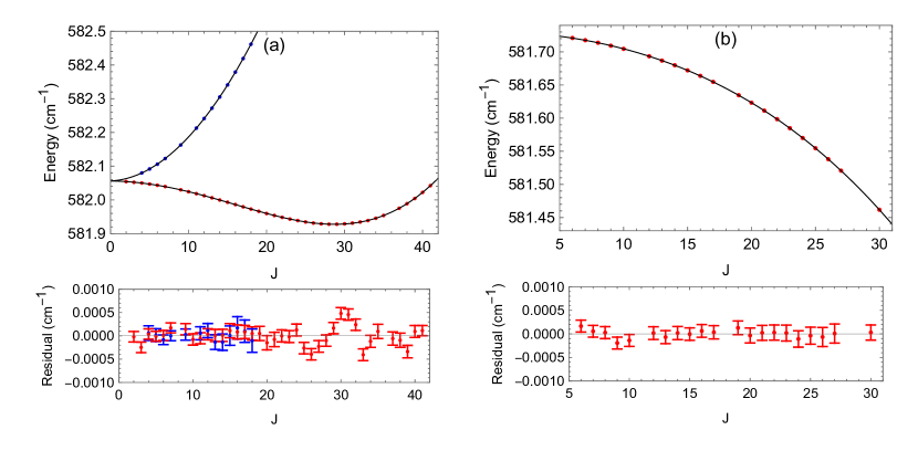
Figure 5: (a) Points: energies of lines in the Q-branch of the $(04^{2}0)-(03^{1}0)$ band; blue/red points have e/f symmetry in the lower level. Lines: fit to Eq. (3). (b) Points: energies of lines in the Q-branch of $(12^{0}0)-(11^{1}0)$; all points have f symmetry in the lower level. Line: fit to Eq. (3). Residuals are shown beneath each plot.

4 Conclusions

Using a quantum cascade laser near 17 $\mu$m and wavelength modulation spectroscopy, we have determined the frequencies of 165 vibrational transitions of N₂O. We have presented a model for the lineshape of absorption features in wavelength modulation spectroscopy, and used this model to fit our spectral data. An optical cavity is used to calibrate the relative frequency scale, and a few calibration lines determined previously are used to fix the absolute frequency. This method transfers the precision of the calibration lines onto all other lines. Using our data alongside previous microwave measurements, we determine the band energies of eight vibrational states of N₂O and the rotational parameters of two states where this information was previously absent. These new spectroscopic data can be used to build more accurate line lists of N₂O in this spectral region, refining and extending existing databases.

In the present work, we only measured the relative amplitudes of lines in the spectrum. The absolute spectral line intensities are important for simulating the transmission of light through atmospheres and could be measured in future work by calibrating the pressure of N₂O in the cell.

The frequency uncertainty of the present measurements are dominated by the uncertainties of the calibration lines and drift in the optical cavity used to establish the frequency scale. In most cases, the determination of the line centre makes a negligible contribution to the overall uncertainty at the present level. In future work, this uncertainty could be reduced further by using sub-Doppler spectroscopy techniques. The cavity drift can be eliminated by stabilizing its temperature and pressure, and/or by using a frequency-stabilized laser in the visible to stabilise the cavity length. Ongoing work aims to improve calibration in this spectral region by building a frequency standard based on the fundamental vibrational transition in trapped, ultracold CaF molecules [18]. Standards of this kind could be developed throughout the mid-infrared using the vibrational transitions of a wide range of ultracold molecules [36, 39]. These standards can then be used to improve the precision of sets of spectral lines in common gases such as N₂O, using the methods described in the present work. For example, one QCL could be locked to a vibrational transition in the ultracold molecule, while a second QCL is used for spectroscopy of the type presented here, and their difference frequency measured using heterodyne techniques.

Appendix A Shape of wavelength modulated spectral lines

In this appendix, we derive an expression for the lineshape of an absorption feature obtained from wavelength modulation spectroscopy. Our analysis extends that found in Refs. [47, 48]. It captures the effects of Doppler broadening and pressure broadening, lineshape changes due to the modulation of the frequency, the effect of large optical depth, and the effect of simultaneous intensity and frequency modulation.

Let $\omega$ be the angular frequency of the laser, $\omega_{\rm c}$ the centre frequency of the absorption feature, and $\gamma$ a quantity representing the linewidth of the absorption feature. The laser current is modulated at frequency $\Omega$ and this modulates both the laser intensity and the laser frequency. We introduce a normalized detuning

$$\Delta=(\omega-\omega_{\rm c})/\gamma=\delta-\delta_{\rm m}\cos(\Omega t+\Phi).$$ (4)

Here, $\delta$ is the detuning of the laser averaged over a modulation cycle and $\delta_{\rm m}$ is the modulation amplitude, both normalized to $\gamma$. The intensity of the light transmitted through the absorbing sample is $I_{\rm out}=I_{\rm in}\exp(-\alpha(\Delta))$ where $I_{\rm in}$ is the input intensity and $\alpha$ is the frequency-dependent optical depth of the sample. We assume that the input intensity varies linearly with the frequency, $I_{\rm in}=I_{0}(1+p\delta-q\delta_{\rm m}\cos(\Omega t))$, where $I_{0}$ is the intensity on resonance, $p$ characterizes the intensity change due to a dc (or slowly-varying) offset, and $q$ characterizes the intensity change due to the modulation. $\Phi$ is a phase shift between the modulation of the frequency and the intensity. With these definitions, the transmitted intensity is

$$I_{\rm out}(\delta,t)=I_{0}\left(1+p\delta-q\delta_{\rm m}\cos(\Omega t)\right)\exp(-\alpha(\delta-\delta_{\rm m}\cos(\Omega t+\Phi))).$$ (5)

We choose to re-write this in the form

$$I_{\rm out}(\delta,t)=g_{1}(\delta-\delta_{\rm m}\cos(\Omega t+\Phi))+g_{2}(\delta-\delta_{\rm m}\cos(\Omega t+\Phi)),$$ (6)

where

$$g_{1}(x) =I_{0}px\exp(-\alpha(x))$$ (7)

$$g_{2}(x) =I_{0}c_{2}\exp(-\alpha(x))$$ (8)

and

$$c_{2}=1-2p\delta_{\rm m}\sin(\Phi/2)\sin(\Omega t+\Phi/2)+(p-q)\delta_{\rm m}\cos(\Omega t).$$ (9)

Our aim is to find the component of $I_{\rm out}$ oscillating at frequency $n\Omega$, where $n$ is an integer, since this is the output of the lock-in amplifier. To do this, we first take the Fourier transform of $I_{\rm out}(\delta)$, which we denote $S(\tau)$:

$$S(\tau,t)=[G_{1}(\tau)+G_{2}(\tau)]\exp(-i\delta_{\rm m}\tau\cos(\Omega t+\Phi)).$$ (10)

Here, $G_{1}(\tau)$ and $G_{2}(\tau)$ are the Fourier transforms of $g_{1}(\delta)$ and $g_{2}(\delta)$ and we have used the shift theorem of Fourier transforms. Next, we use the Jacobi-Anger expansion which has the general form $e^{iz\cos\theta}=J_{0}(z)+2\sum_{n=1}^{\infty}i^{n}J_{n}(z)\cos(n\theta)$, where $J_{n}$ is the Bessel function of the first kind. Applying this to Eq.(10) and using $J_{n}(-z)=(-1)^{n}J_{n}(z)$ we get

$$S(\tau,t)=[G_{1}(\tau)+G_{2}(\tau)]\sum_{n=0}^{\infty}\epsilon_{n}(-i)^{n}J_{n}(\delta_{\rm m}\tau)\cos[n(\Omega t+\Phi)],$$ (11)

where $\epsilon_{0}=1$ and $\epsilon_{n}=2$ for all $n>0$. We now take the inverse Fourier transform, noting that the cosine factor does not depend on $\tau$, to obtain

$$I_{\rm out}(\delta,t)=s_{1}(\delta,t)+s_{2}(\delta,t)$$ (12)

where

$$s_{k}(\delta,t)=\sum_{n=0}^{\infty}s_{k,n}(\delta)\cos[n(\Omega t+\Phi)],$$ (13)

and

$$s_{k,n}(\delta)=\epsilon_{n}(-i)^{n}\frac{1}{2\pi}\int_{-\infty}^{\infty}e^{i\delta\tau}J_{n}(\delta_{\rm m}\tau)G_{k}(\tau)d\tau.$$ (14)

The integral in Eq. (14) is the inverse Fourier transform of the product of $J_{n}$ and $G_{k}$. Applying the convolution theorem, this can be written as

$$s_{k,n}(\delta)=\epsilon_{n}(-i)^{n}\frac{1}{\delta_{\rm m}}\int_{-\infty}^{\infty}j_{n}\left(\frac{\delta^{\prime}}{\delta_{\rm m}}\right)g_{k}(\delta-\delta^{\prime})d\delta^{\prime},$$ (15)

where $j_{n}$ is the Fourier transform of the Bessel function, $j_{n}(x)=2(-i)^{n}\cos(n\cos^{-1}(x))/\sqrt{1-x^{2}}$ for $|x|<1$ and zero otherwise. So we have

$$s_{k,n}(\delta)=2\epsilon_{n}(-1)^{n}\int_{-\delta_{\rm m}}^{\delta_{\rm m}}\frac{\cos(n\cos^{-1}(\delta^{\prime}/\delta_{\rm m}))}{\sqrt{\delta_{\rm m}^{2}-\delta^{\prime 2}}}g_{k}(\delta-\delta^{\prime})d\delta^{\prime}.$$ (16)

The decomposition into a sum of harmonics of $\Omega$ is complicated by the presence of trigonometric functions of $\Omega t$ in the expression for $c_{2}$, Eq. (9). This can be sorted out using

$$c_{2}\cos[n(\Omega T+\Phi)]=\cos[n(\Omega T+\Phi)]$$

$$+\frac{1}{2}\delta_{m}p\left(\cos[(n-1)(\Omega T+\Phi)]+\cos[(n+1)(\Omega T+\Phi)]\right)$$

$$-\frac{1}{2}\delta_{m}q\left(\cos[(n-1)\Omega T+n\Phi]+\cos[(n+1)\Omega T+n\Phi]\right).$$ (17)

This shows that the term oscillating at $n\Omega$ will have contributions from $s_{2,n\pm 1}$ as well as from $s_{2,n}$.

These equations can be used to determine the lineshape in the most general cases. In the case where the intensity and frequency oscillate in phase ($\Phi=0$) and the intensity changes in the same way for slow and fast changes ($p=q$), the result simplifies because $c_{2}=1$. In this case, the component of the output signal oscillating at frequency $n\Omega$ is

$$\frac{I_{{\rm out},n}}{I_{0}}=2\epsilon_{n}(-1)^{n}\int_{-\delta_{\rm m}}^{\delta_{\rm m}}\frac{\cos\left(n\cos^{-1}\left(\frac{\delta^{\prime}}{\delta_{\rm m}}\right)\right)}{\sqrt{\delta_{\rm m}^{2}-\delta^{\prime 2}}}(1+p\delta-p\delta^{\prime})e^{-\alpha(\delta-\delta^{\prime})}d\delta^{\prime}.$$ (18)

The function $\alpha(\delta)$ should be chosen according to the dominant broadening mechanisms. In this paper, we have used the Voigt function. We found Eq. (18) to be an adequate representation of the lineshapes we measure across the full range of optical depths. We note that others have used expressions that avoid the two assumptions ($\Phi=0$, $p=q$) used above [48, 14].

Appendix B Frequency uncertainties

We record the N₂O spectrum and the cavity transmission simultaneously, giving two sets of data with a common abscissa. The abscissa may be the QCL current, or it may be time since the current is scanned linearly - we will call it $t$. The laser frequency is a function of $t$ but may not be a perfectly linear function. We fit to the cavity transmission data to get the cavity phase as a function of $t$, which is proportional to the laser frequency, $\phi(t)=\alpha f(t)+\theta$. We use three calibration lines, but for any line in the spectrum we only use the two closest calibration lines. They have frequencies $f_{i}$ and corresponding cavity phases $\phi_{i}$, with $\phi_{i}=\alpha f_{i}+\theta$. With these definitions, the frequency can be expressed as

$$f(t)=\frac{f_{1}(\phi_{2}-\phi(t))-f_{2}(\phi_{1}-\phi(t))}{\phi_{2}-\phi_{1}}.$$ (19)

From Eq. (19) we find the frequency uncertainty to be

$$\sigma_{f}=\sqrt{\sum_{i=1}^{2}\left(\frac{\phi-\phi_{i}}{\phi_{2}-\phi_{1}}\right)^{2}(\sigma_{f_{i}}^{2}+\beta^{2}\sigma_{\phi_{i}}^{2})+\beta^{2}\sigma_{\phi}^{2}+\beta^{2}\left(\frac{d\phi}{dt}\right)^{2}\sigma_{t}^{2}},$$ (20)

where $\beta=\frac{f_{2}-f_{1}}{\phi_{2}-\phi_{1}}$. Here, $\sigma_{f_{1}}$ and $\sigma_{f_{2}}$ are the frequency uncertainties in the two calibration lines, $\sigma_{\phi_{1}}$ and $\sigma_{\phi_{2}}$ are the uncertainties in the cavity phases at the two calibration lines, $\sigma_{\phi}$ is the uncertainty in the cavity phase at the spectral line being measured, and $\sigma_{t}$ is the uncertainty in determining the line centre of the spectral line on the $t$-axis.

In addition, we need to account for the uncertainty from the drift of the cavity’s optical path length, which arises due to changes in temperature and pressure. Let us first suppose that the cavity length drifts linearly in time at a rate $\gamma$, and the frequency is scanned linearly in time. Recognizing that the cavity phase is proportional to the frequency of the light multiplied by the length of the cavity, we find that Eq. (19) is modified to

$$f(t)=\frac{f_{1}(t_{2}-t)(L+\gamma t_{1})-f_{2}(t_{1}-t)(L+\gamma t_{2})}{(t_{2}-t_{1})(L+\gamma t)},$$ (21)

where $L$ is the nominal length of the cavity and $t_{1,2}$ are the times in the scan where the calibration lines appear. We treat the cavity drift as an uncertainty by assuming that its mean value is zero but its variance is not. This leads to a frequency uncertainty due to cavity drift of

$$\sigma_{f}=\frac{(f_{2}-f_{1})}{(t_{2}-t_{1})}(t-t_{1})(t_{2}-t)\frac{1}{L}\sigma_{\gamma}.$$ (22)

We monitored the frequency drift of the cavity and observed a drift of 30 kHz/s. This translates to $\sigma_{f}<2$ kHz, which is negligible. The uncertainty is tiny because the calibration procedure almost eliminates the effect of the drift when both the drift and the frequency scan are linear in time. The scan is not quite linear, but the non-linearity is small enough that the uncertainty remains negligible.

To produce a significant effect, the cavity has to drift in a different way. For example, suppose that in scanning from $f_{1}$ to $f_{2}$, the cavity length expands linearly during the first half of the scan and then contracts linearly during the second half so as to return to its original length by the end of the scan. This conspiratorial behaviour produces a much larger effect. The uncertainty is

$$\sigma_{f}=\tau|\sigma_{\frac{df}{dt}}|$$ (23)

where $\frac{df}{dt}$ is the drift of the cavity resonance frequency and $\tau$ is the time to/from the nearest calibration line, i.e. $(t-t_{1})$ or $(t_{2}-t)$, whichever is smaller. A sudden step change in the length of the cavity part way through a scan has a similar effect.

Appendix C Table of frequencies

Table 3: A complete table of measured N₂O transitions. The columns are as follows. iso: a code used in HITRAN [22] to identify the isotope of N₂O; 41 means ¹⁴N${}_{2}^{16}$O, 42 means ¹⁴N¹⁵N¹⁶O, 43 means ¹⁵N¹⁴N¹⁶O, 44 means ¹⁴N${}_{2}^{18}$O and 45 means ¹⁴N${}_{2}^{17}$O. wn (observed): our measured wavenumbers (in cm^-1) with 2$\sigma$ uncertainties given in parentheses. wn (hi): transition wavenumbers listed in HITRAN (in cm^-1). wn (nist): transition wavenumbers listed as calibration lines by NIST (in cm^-1). ‘o-ht’: difference between our measured wavenumbers and those in HITRAN (in cm^-1). o-nist: difference between our measured wavenumbers and those in NIST database (in cm^-1). $f$ (observed): our measured frequency (in THz). $v_{1}^{\prime},v_{2}^{\prime},l^{\prime},v_{3}^{\prime}$: vibrational quantum numbers of upper state. $v_{1},v_{2},l,v_{3}$: vibrational quantum numbers of lower state. PQR: type of rotational transition. $J^{\prime}$: rotational quantum number of upper state. $J$: rotational quantum number of lower state. p: e/f symmetry of the lower level. ov: whether the line is overlapped with other lines; s means no overlap and o means overlap. amp: fitted amplitude value using Voigt line profile.

iso	wn (observed)	wn (ht)	wn (nist)	o-ht	o-nist	f(observed)	v1’	v2’	l’	v3’	v1	v2	l	v3	PQR	J’	J	p	ov	amp
44	580.272780(098)	580.27260		0.000180		17.3961403	0	1	1	0	0	0	0	0	P	4	5	e	s	0.0039
41	580.294380(101)	580.29432		0.000060		17.3967879	0	4	0	0	0	3	1	0	R	8	7	e	s	0.0004
41	580.403216(098)	580.40323	580.403216	-0.000015	0.000000	17.4000507	0	1	1	0	0	0	0	0	P	9	10	e	s	1.6335
41	580.409019(099)	580.40913	580.409125	-0.000111	-0.000106	17.4002246	1	1	1	0	1	0	0	0	P	17	18	e	s	0.0051
43	580.459383(102)	580.45934		0.000043		17.4017345	0	1	1	0	0	0	0	0	P	5	6	e	s	0.0019
42	580.466629(102)	580.46661		0.000019		17.4019518	0	1	1	0	0	0	0	0	R	6	5	e	s	0.0024
41	580.489628(116)	580.48964		-0.000012		17.4026412	0	3	1	0	0	2	2	0	R	11	10	e	s	0.0012
41	580.591669(134)	580.59218		-0.000511		17.4057004	0	2	2	0	0	1	1	0	P	9	10	f	s	0.0824
42	580.640513(130)	580.64099		-0.000477		17.4071647	0	2	2	0	0	1	1	0	R	6	5	f	s	0.0003
42	580.665053(129)	580.66533		-0.000277		17.4079003	0	2	2	0	0	1	1	0	R	6	5	e	s	0.0001
45	580.676511(137)	580.67613		0.000381		17.4082439	0	1	1	0	0	0	0	0	P	6	7	e	s	0.0006
41	580.679905(120)	580.67969		0.000215		17.4083456	0	2	2	0	0	1	1	0	P	9	10	e	s	0.0820
41	580.687841(120)	580.68743		0.000411		17.4085835	0	3	1	0	0	2	2	0	R	11	10	f	s	0.0015
42	580.798609(122)	580.79890		-0.000291		17.4119043	0	2	0	0	0	1	1	0	R	14	13	e	s	0.0001
41	580.814320(111)	580.81411		0.000210		17.4123753	0	3	3	0	0	2	2	0	P	9	10	e	o	0.0045
41	580.814320(111)	580.81494		-0.000620		17.4123753	0	3	3	0	0	2	2	0	P	9	10	f	o	0.0045
41	580.935105(106)	580.93517		-0.000065		17.4159963	0	3	1	0	0	2	0	0	Q	1	1	e	s	0.0018
41	580.939720(105)	580.93980		-0.000080		17.4161347	0	3	1	0	0	2	0	0	Q	2	2	e	s	0.0046
41	580.946644(105)	580.94675		-0.000106		17.4163422	0	3	1	0	0	2	0	0	Q	3	3	e	s	0.0103
41	580.955991(105)	580.95602		-0.000029		17.4166225	0	3	1	0	0	2	0	0	Q	4	4	e	s	0.0103
41	580.967635(103)	580.96762		0.000015		17.4169715	0	3	1	0	0	2	0	0	Q	5	5	e	s	0.0119
41	580.975060(110)	580.97595		-0.000890		17.4171941	0	4	4	0	0	3	3	0	P	9	10	f	s	0.0030
41	580.977014(119)	580.97621		0.000804		17.4172527	0	4	4	0	0	3	3	0	P	9	10	e	s	0.0019
41	580.981594(102)	580.98155		0.000044		17.4173900	0	3	1	0	0	2	0	0	Q	6	6	e	s	0.0170
41	580.997890(103)	580.99780		0.000090		17.4178786	0	3	1	0	0	2	0	0	Q	7	7	e	s	0.0180
41	581.016500(102)	581.01640		0.000100		17.4184365	0	3	1	0	0	2	0	0	Q	8	8	e	s	0.0187
41	581.037390(101)	581.03733		0.000060		17.4190627	0	3	1	0	0	2	0	0	Q	9	9	e	s	0.0202
41	581.045788(101)	581.04559	581.045815	0.000198	-0.000027	17.4193145	0	2	0	0	0	1	1	0	R	2	1	e	s	0.0103
41	581.060616(115)	581.06062		-0.000004		17.4197590	0	3	1	0	0	2	0	0	Q	10	10	e	s	0.0240
44	581.062542(117)	581.06226		0.000282		17.4198168	0	1	1	0	0	0	0	0	P	3	4	e	s	0.0006
41	581.065240(131)	581.06450		0.000740		17.4198977	0	4	2	0	0	3	3	0	R	20	19	f	s	0.0016
41	581.086009(105)	581.08626		-0.000251		17.4205203	0	3	1	0	0	2	0	0	Q	11	11	e	s	0.0276
41	581.094567(114)	581.09753		-0.002963		17.4207769	0	4	2	0	0	3	3	0	R	20	19	e	s	0.0005
41	581.114122(102)	581.11427		-0.000148		17.4213631	0	3	1	0	0	2	0	0	Q	12	12	e	s	0.0257
41	581.144577(101)	581.14465		-0.000073		17.4222761	0	3	1	0	0	2	0	0	Q	13	13	e	s	0.0254
41	581.151653(105)	581.15140		0.000253		17.4224883	0	4	0	0	0	3	1	0	R	9	8	e	s	0.0011
41	581.177273(103)	581.17741		-0.000137		17.4232563	0	3	1	0	0	2	0	0	Q	14	14	e	s	0.0270
41	581.185699(117)	581.18565		0.000049		17.4235089	1	2	2	0	1	1	1	0	P	15	16	f	s	0.0007
43	581.187960(119)	581.18819		-0.000230		17.4235767	0	2	0	0	0	1	1	0	R	8	7	e	s	0.0020
41	581.212526(099)	581.21257		-0.000044		17.4243132	0	3	1	0	0	2	0	0	Q	15	15	e	s	0.0278
41	581.236040(128)	581.23593	581.235921	0.000110	0.000119	17.4250183	1	1	1	0	1	0	0	0	P	16	17	e	s	0.0094
41	581.238050(109)	581.23806	581.238050	-0.000014	0.000000	17.4250784	0	1	1	0	0	0	0	0	P	8	9	e	s	1.4866
41	581.250108(110)	581.25012		-0.000012		17.4254399	0	3	1	0	0	2	0	0	Q	16	16	e	s	0.0274
43	581.267218(096)	581.26721		0.000008		17.4259528	0	1	1	0	0	0	0	0	P	4	5	e	s	0.0031
41	581.290115(096)	581.29009		0.000025		17.4266392	0	3	1	0	0	2	0	0	Q	17	17	e	s	0.0300
42	581.306275(097)	581.30626		0.000015		17.4271237	0	1	1	0	0	0	0	0	R	7	6	e	s	0.0071
41	581.316089(097)	581.31608		0.000009		17.4274179	0	3	1	0	0	2	2	0	R	12	11	e	s	0.0030
41	581.332543(097)	581.33247		0.000073		17.4279112	0	3	1	0	0	2	0	0	Q	18	18	e	s	0.0282
41	581.377275(099)	581.37730		-0.000025		17.4292522	0	3	1	0	0	2	0	0	Q	19	19	e	s	0.0311
41	581.424507(100)	581.42457		-0.000063		17.4306682	0	3	1	0	0	2	0	0	Q	20	20	e	s	0.0360
41	581.428922(100)	581.42911		-0.000188		17.4308006	0	2	2	0	0	1	1	0	P	8	9	f	s	0.0855
41	581.461740(107)	581.46176		-0.000020		17.4317844	1	2	0	0	1	1	1	0	Q	30	30	f	s	0.0026
41	581.474371(103)	581.47429		0.000081		17.4321631	0	3	1	0	0	2	0	0	Q	21	21	e	s	0.0285
42	581.482067(110)	581.48236		-0.000293		17.4323938	0	2	2	0	0	1	1	0	R	7	6	f	s	0.0006
45	581.487453(118)	581.48729		0.000163		17.4325553	0	1	1	0	0	0	0	0	P	5	6	e	s	0.0001
41	581.500515(106)	581.50063		-0.000115		17.4329469	0	2	2	0	0	1	1	0	P	8	9	e	s	0.0895
42	581.515805(120)	581.51650	581.515805	-0.000695		17.4334053	0	2	2	0	0	1	1	0	R	7	6	e	s	0.0001
41	581.520688(122)	581.52091		-0.000222		17.4335516	1	2	0	0	1	1	1	0	Q	27	27	f	s	0.0001
41	581.526320(106)	581.52649		-0.000170		17.4337205	0	3	1	0	0	2	0	0	Q	22	22	e	s	0.0248
41	581.538106(126)	581.53846		-0.000354		17.4340738	1	2	0	0	1	1	1	0	Q	26	26	f	s	0.0002
41	581.549688(103)	581.55002		-0.000332		17.4344210	0	3	1	0	0	2	2	0	R	12	11	f	s	0.0030
41	581.554614(104)	581.55499		-0.000376		17.4345687	1	2	0	0	1	1	1	0	Q	25	25	f	s	0.0003
41	581.570054(104)	581.57055		-0.000496		17.4350316	1	2	0	0	1	1	1	0	Q	24	24	f	s	0.0001
41	581.580833(102)	581.58116		-0.000327		17.4353547	0	3	1	0	0	2	0	0	Q	23	23	e	s	0.0173
41	581.584758(104)	581.58517		-0.000412		17.4354724	1	2	0	0	1	1	1	0	Q	23	23	f	s	0.0005
41	581.598454(104)	581.59890		-0.000446		17.4358830	1	2	0	0	1	1	1	0	Q	22	22	f	s	0.0001
41	581.611277(105)	581.61176		-0.000483		17.4362674	1	2	0	0	1	1	1	0	Q	21	21	f	s	0.0002
41	581.623229(114)	581.62379		-0.000561		17.4366258	1	2	0	0	1	1	1	0	Q	20	20	f	s	0.0001
41	581.634609(101)	581.63502		-0.000411		17.4369669	1	2	0	0	1	1	1	0	Q	19	19	f	s	0.0004
41	581.638073(101)	581.63833		-0.000257		17.4370707	0	3	1	0	0	2	0	0	Q	24	24	e	s	0.0187
41	581.644333(101)	581.64460		-0.000267		17.4372584	0	3	3	0	0	2	2	0	P	8	9	e	o	0.0071
41	581.644333(101)	581.64520		-0.000867		17.4372584	0	3	3	0	0	2	2	0	P	8	9	f	o	0.0071
41	581.654709(104)	581.65522		-0.000511		17.4375695	1	2	0	0	1	1	1	0	Q	17	17	f	s	0.0001
42	581.659056(103)	581.65965		-0.000594		17.4376998	0	2	0	0	0	1	1	0	R	15	14	e	s	0.0001
41	581.663774(102)	581.66426		-0.000486		17.4378413	1	2	0	0	1	1	1	0	Q	16	16	f	s	0.0010
41	581.672070(104)	581.67261		-0.000540		17.4380899	1	2	0	0	1	1	1	0	Q	15	15	f	s	0.0001
41	581.679809(115)	581.68031		-0.000501		17.4383220	1	2	0	0	1	1	1	0	Q	14	14	f	s	0.0002
41	581.686818(115)	581.68739		-0.000572		17.4385321	1	2	0	0	1	1	1	0	Q	13	13	f	s	0.0002
41	581.693398(115)	581.69386		-0.000462		17.4387294	1	2	0	0	1	1	1	0	Q	12	12	f	s	0.0005
41	581.697576(115)	581.69801		-0.000434		17.4388546	0	3	1	0	0	2	0	0	Q	25	25	e	s	0.0158
41	581.704514(107)	581.70508		-0.000566		17.4390626	1	2	0	0	1	1	1	0	Q	10	10	f	s	0.0015
41	581.709271(108)	581.70986		-0.000589		17.4392052	1	2	0	0	1	1	1	0	Q	9	9	f	s	0.0002
41	581.713778(111)	581.71412		-0.000342		17.4393403	1	2	0	0	1	1	1	0	Q	8	8	f	s	0.0001
41	581.717580(110)	581.71787		-0.000290		17.4394543	1	2	0	0	1	1	1	0	Q	7	7	f	s	0.0001
41	581.720964(113)	581.72112		-0.000156		17.4395558	1	2	0	0	1	1	1	0	Q	6	6	f	s	0.0001
41	581.759976(097)	581.76021		-0.000234		17.4407253	0	3	1	0	0	2	0	0	Q	26	26	e	s	0.0157
41	581.771556(097)	581.77210		-0.000544		17.4410725	0	3	1	0	0	2	0	0	R	1	0	e	s	0.0021
41	581.806173(105)	581.80751		-0.001337		17.4421103	0	4	4	0	0	3	3	0	P	8	9	f	o	0.0002
41	581.806173(105)	581.80771		-0.001537		17.4421103	0	4	4	0	0	3	3	0	P	8	9	e	o	0.0002
41	581.824473(096)	581.82494		-0.000467		17.4426589	0	3	1	0	0	2	0	0	Q	27	27	e	s	0.0149
44	581.852146(098)	581.85230		-0.000154		17.4434885	0	1	1	0	0	0	0	0	P	2	3	e	s	0.0003
41	581.888125(099)	581.88838	581.888602	-0.000255	-0.000477	17.4445671	0	2	0	0	0	1	1	0	R	3	2	e	s	0.0256
41	581.891909(099)	581.89222		-0.000311		17.4446806	0	3	1	0	0	2	0	0	Q	28	28	e	s	0.0146
41	581.927927(106)	581.92818		-0.000253		17.4457604	0	4	2	0	0	3	1	0	Q	29	29	f	o	0.0007
41	581.927927(106)	581.92841		-0.000483		17.4457604	0	4	2	0	0	3	1	0	Q	28	28	f	o	0.0007
41	581.929121(111)	581.92910		0.000021		17.4457962	0	4	2	0	0	3	1	0	Q	30	30	f	o	0.0010
41	581.929121(111)	581.92969		-0.000569		17.4457962	0	4	2	0	0	3	1	0	Q	27	27	f	o	0.0010
41	581.931220(107)	581.93126		-0.000040		17.4458591	0	4	2	0	0	3	1	0	Q	31	31	f	o	0.0027
41	581.931220(107)	581.93192		-0.000700		17.4458591	0	4	2	0	0	3	1	0	Q	26	26	f	o	0.0027
41	581.934474(106)	581.93477		-0.000296		17.4459566	0	4	2	0	0	3	1	0	Q	32	32	f	o	0.0031
41	581.934474(106)	581.93501		-0.000536		17.4459566	0	4	2	0	0	3	1	0	Q	25	25	f	o	0.0031
41	581.938744(109)	581.93886		-0.000116		17.4460847	0	4	2	0	0	3	1	0	Q	24	24	f	o	0.0013
41	581.938744(109)	581.93972		-0.000976		17.4460847	0	4	2	0	0	3	1	0	Q	33	33	f	o	0.0013
41	581.943147(109)	581.94338		-0.000233		17.4462167	0	4	2	0	0	3	1	0	Q	23	23	f	s	0.0015
41	581.945491(109)	581.94620		-0.000709		17.4462869	0	4	2	0	0	3	1	0	Q	34	34	f	o	0.0009
41	581.945491(109)	581.94731		-0.001819		17.4462869	0	4	2	0	0	3	3	0	R	21	20	e	o	0.0009
41	581.948281(109)	581.94848		-0.000199		17.4463705	0	4	2	0	0	3	1	0	Q	22	22	f	s	0.0005
41	581.953805(138)	581.95406		-0.000255		17.4465362	0	4	2	0	0	3	1	0	Q	21	21	f	o	0.0007
41	581.953805(138)	581.95432		-0.000515		17.4465362	0	4	2	0	0	3	1	0	Q	35	35	f	o	0.0007
41	581.959731(139)	581.96005		-0.000319		17.4467138	0	4	2	0	0	3	1	0	Q	20	20	f	s	0.0002
41	581.961634(139)	581.96205		-0.000416		17.4467709	0	3	1	0	0	2	0	0	Q	29	29	e	s	0.0117
41	581.966237(140)	581.96634		-0.000103		17.4469089	0	4	2	0	0	3	1	0	Q	19	19	f	s	0.0023
41	581.972770(130)	581.97287		-0.000100		17.4471047	0	4	2	0	0	3	1	0	Q	18	18	f	s	0.0004
41	581.975167(131)	581.97582		-0.000653		17.4471766	0	4	2	0	0	3	1	0	Q	37	37	f	s	0.0005
41	581.979488(131)	581.97955		-0.000062		17.4473061	0	4	2	0	0	3	1	0	Q	17	17	f	s	0.0005
41	581.986243(144)	581.98631		-0.000067		17.4475086	0	4	2	0	0	3	1	0	Q	16	16	f	s	0.0005
41	581.988735(144)	581.98938		-0.000645		17.4475833	0	4	2	0	0	3	1	0	Q	38	38	f	s	0.0005
41	581.993025(144)	581.99307		-0.000045		17.4477120	0	4	2	0	0	3	1	0	Q	15	15	f	s	0.0005
41	581.999609(123)	581.99976		-0.000151		17.4479093	0	4	2	0	0	3	1	0	Q	14	14	f	s	0.0006
41	582.004116(128)	582.00494		-0.000824		17.4480444	0	4	2	0	0	3	1	0	Q	39	39	f	s	0.0002
41	582.006152(124)	582.00631		-0.000158		17.4481055	0	4	2	0	0	3	1	0	Q	13	13	f	s	0.0006
43	582.009828(114)	582.01011		-0.000282		17.4482157	0	2	0	0	0	1	1	0	R	9	8	e	o	0.0012
41	582.009828(114)	582.01031		-0.000482		17.4482157	0	4	0	0	0	3	1	0	R	10	9	e	o	0.0012
41	582.012527(114)	582.01267		-0.000143		17.4482966	0	4	2	0	0	3	1	0	Q	12	12	f	s	0.0011
41	582.017092(115)	582.01719		-0.000098		17.4484335	1	2	2	0	1	1	1	0	P	14	15	f	s	0.0015
41	582.018532(114)	582.01877		-0.000238		17.4484766	0	4	2	0	0	3	1	0	Q	11	11	f	s	0.0008
41	582.022284(123)	582.02257		-0.000286		17.4485891	0	4	2	0	0	3	1	0	Q	40	40	f	s	0.0017
41	582.024284(118)	582.02456		-0.000276		17.4486491	0	4	2	0	0	3	1	0	Q	10	10	f	s	0.0008
41	582.029921(118)	582.02998		-0.000059		17.4488181	0	4	2	0	0	3	1	0	Q	9	9	f	s	0.0005
41	582.034291(117)	582.03446		-0.000169		17.4489491	0	3	1	0	0	2	0	0	Q	30	30	e	s	0.0122
41	582.039516(105)	582.03957		-0.000054		17.4491057	0	4	2	0	0	3	1	0	Q	7	7	f	s	0.0004
41	582.042234(107)	582.04236		-0.000126		17.4491872	0	4	2	0	0	3	1	0	Q	41	41	f	s	0.0008
41	582.043426(107)	582.04365		-0.000224		17.4492229	0	4	2	0	0	3	1	0	Q	6	6	f	s	0.0014
41	582.046956(107)	582.04721		-0.000254		17.4493287	0	4	2	0	0	3	1	0	Q	5	5	f	s	0.0018
41	582.050008(111)	582.05022		-0.000212		17.4494203	0	4	2	0	0	3	1	0	Q	4	4	f	s	0.0022
41	582.052152(113)	582.05266		-0.000508		17.4494845	0	4	2	0	0	3	1	0	Q	3	3	f	s	0.0014
41	582.054220(113)	582.05450		-0.000280		17.4495465	0	4	2	0	0	3	1	0	Q	2	2	f	s	0.0002
41	582.063118(105)	582.06321	582.063199	-0.000092	-0.000081	17.4498133	1	1	1	0	1	0	0	0	P	15	16	e	s	0.0025
41	582.073253(104)	582.07327	582.073253	-0.000014	0.000000	17.4501171	0	1	1	0	0	0	0	0	P	7	8	e	s	1.3931
41	582.079876(155)	582.07998		-0.000104		17.4503157	0	4	2	0	0	3	1	0	Q	4	4	e	s	0.0011
41	582.091695(137)	582.09186		-0.000165		17.4506700	0	4	2	0	0	3	1	0	Q	5	5	e	s	0.0006
41	582.105832(102)	582.10612		-0.000288		17.4510938	0	4	2	0	0	3	1	0	Q	6	6	e	s	0.0014
41	582.109215(101)	582.10945		-0.000235		17.4511952	0	3	1	0	0	2	0	0	Q	31	31	e	s	0.0128
41	582.122526(103)	582.12275		-0.000224		17.4515943	0	4	2	0	0	3	1	0	Q	7	7	e	s	0.0003
41	582.141047(105)	582.14124		-0.000193		17.4521495	0	3	1	0	0	2	2	0	R	13	12	e	s	0.0016
42	582.145835(105)	582.14614		-0.000305		17.4522931	0	1	1	0	0	0	0	0	R	8	7	e	s	0.0052
41	582.162889(108)	582.16313		-0.000241		17.4528043	0	4	2	0	0	3	1	0	Q	9	9	e	s	0.0004
41	582.186785(112)	582.18703		-0.000245		17.4535207	0	3	1	0	0	2	0	0	Q	32	32	e	s	0.0123
41	582.212747(114)	582.21299		-0.000243		17.4542990	0	4	2	0	0	3	1	0	Q	11	11	e	s	0.0007
41	582.241277(116)	582.24147		-0.000193		17.4551544	0	4	2	0	0	3	1	0	Q	12	12	e	s	0.0011
41	582.265908(108)	582.26640		-0.000492		17.4558928	0	2	2	0	0	1	1	0	P	7	8	f	s	0.0603
41	582.266871(109)	582.26721		-0.000339		17.4559216	0	3	1	0	0	2	0	0	Q	33	33	e	s	0.0066
41	582.271872(110)	582.27232		-0.000448		17.4560716	0	4	2	0	0	3	1	0	Q	13	13	e	s	0.0040
41	582.305078(114)	582.30553		-0.000452		17.4570671	0	4	2	0	0	3	1	0	Q	14	14	e	s	0.0015
41	582.323201(132)	582.32355		-0.000349		17.4576104	0	2	2	0	0	1	1	0	P	7	8	e	s	0.0553
41	582.340790(138)	582.34111		-0.000320		17.4581377	0	4	2	0	0	3	1	0	Q	15	15	e	s	0.0004
41	582.349705(134)	582.35002		-0.000315		17.4584049	0	3	1	0	0	2	0	0	Q	34	34	e	s	0.0037
42	582.369249(180)	582.36954		-0.000291		17.4589909	0	2	2	0	0	1	1	0	R	8	7	e	s	0.0002
41	582.378885(177)	582.37905		-0.000165		17.4592797	0	4	2	0	0	3	1	0	Q	16	16	e	s	0.0004
41	582.414368(150)	582.41438		-0.000012		17.4603435	0	3	1	0	0	2	2	0	R	13	12	f	s	0.0011
41	582.419100(152)	582.41935		-0.000250		17.4604854	0	4	2	0	0	3	1	0	Q	17	17	e	s	0.0011
41	582.435321(153)	582.43544		-0.000119		17.4609716	0	3	1	0	0	2	0	0	Q	35	35	e	s	0.0025
41	582.461529(138)	582.46200		-0.000471		17.4617573	0	4	2	0	0	3	1	0	Q	18	18	e	s	0.0002
41	582.475740(134)	582.47616		-0.000420		17.4621834	0	3	3	0	0	2	2	0	P	7	8	e	o	0.0027
41	582.475740(134)	582.47649		-0.000750		17.4621834	0	3	3	0	0	2	2	0	P	7	8	f	o	0.0027

References

- [1] A. Kosterev, G. Wysocki, Y. Bakhirkin, S. So, R. Lewicki, M. Fraser, F. Tittel, and R.F. Curl. Application of quantum cascade lasers to trace gas analysis. Appl. Phys. B, 90:165–176, 2008.
- [2] Iacopo Galli, Saverio Bartalini, Riccardo Ballerini, Marco Barucci, Pablo Cancio, Marco De Pas, Giovanni Giusfredi, Davide Mazzotti, Naota Akikusa, and Paolo De Natale. Spectroscopic detection of radiocarbon dioxide at parts-per-quadrillion sensitivity. Optica, 3:385–388, 2016.
- [3] Pedro Martín-Mateos, Jakob Hayden, Pablo Acedo, and Bernhard Lendl. Heterodyne Phase-Sensitive Dispersion Spectroscopy in the Mid-Infrared with a Quantum Cascade Laser. Anal. Chem., 89:5916–5922, 2017.
- [4] Nart S. Daghestani, Richard Brownsword, and Damien Weidmann. Analysis and demonstration of atmospheric methane monitoring by mid-infrared open-path chirped laser dispersion spectroscopy. Opt. Express, 22:A1731–A1743, 2014.
- [5] Iain Robinson, Helen L. Butcher, Neil A. Macleod, and Damien Weidmann. Hollow waveguide-miniaturized quantum cascade laser heterodyne spectro-radiometer. Opt. Express, 29:2299–2308, 2021.
- [6] Franck Bielsa, Khelifa Djerroud, Andrei Goncharov, Albane Douillet, Tristan Valenzuela, Christophe Daussy, Laurent Hilico, and Anne Amy-Klein. HCOOH high-resolution spectroscopy in the 9.18μm region. J. Mol. Spectrosc., 247:41–46, 2008.
- [7] Simone Borri, Giacomo Insero, Gabriele Santambrogio, Davide Mazzotti, Francesco Cappelli, Iacopo Galli, Gianluca Galzerano, Marco Marangoni, Paolo Laporta, Valentina Di Sarno, Luigi Santamaria, Pasquale Maddaloni, and Paolo De Natale. High-precision molecular spectroscopy in the mid-infrared using quantum cascade lasers. Appl. Phys. B, 125:18, 2019.
- [8] D. D’Ambrosio, S. Borri, M. Verde, A. Borgognoni, G. Insero, P. De Natale, and G. Santambrogio. Approaching the transit time limit for high-precision spectroscopy on metastable CO around 6 μm. Phys. Chem. Chem. Phys., 21:24506–24511, 2019.
- [9] Pierre Asselin, Yann Berger, Thérèse R. Huet, Laurent Margulès, Roman Motiyenko, Richard J. Hendricks, Michael R. Tarbutt, Sean K. Tokunaga, and Benoît Darquié. Characterising molecules for fundamental physics: an accurate spectroscopic model of methyltrioxorhenium derived from new infrared and millimetre-wave measurements. Phys. Chem. Chem. Phys., 19:4576–4587, 2017.
- [10] P. L. T. Sow, S. Mejri, S. K. Tokunaga, O. Lopez, A. Goncharov, B. Argence, C. Chardonnet, A. Amy-Klein, C. Daussy, and B. Darquié. A widely tunable 10-μm quantum cascade laser phase-locked to a state-of-the-art mid-infrared reference for precision molecular spectroscopy. Appl. Phys. Lett., 104:264101, 2014.
- [11] Michael G. Hansen, Evangelos Magoulakis, Qun-Feng Chen, Ingo Ernsting, and Stephan Schiller. Quantum cascade laser-based mid-ir frequency metrology system with ultra-narrow linewidth and level frequency instability. Opt. Lett., 40:2289–2292, 2015.
- [12] Bérengère Argence, Bruno Chanteau, Olivier Lopez, Daniele Nicolodi, Michel Abgrall, Christian Chardonnet, Christophe Daussy, Benoît Darquié, Yann Le Coq, and Anne Amy-Klein. Quantum cascade laser frequency stabilization at the sub-Hz level. Nat. Phot., 9:456–460, 2015.
- [13] R. Santagata, D. B. A. Tran, B. Argence, O. Lopez, S. K. Tokunaga, F. Wiotte, H. Mouhamad, A. Goncharov, M. Abgrall, Y. Le Coq, H. Alvarez-Martinez, R. Le Targat, W. K. Lee, D. Xu, P.-E. Pottie, B. Darquié, and A. Amy-Klein. High-precision methanol spectroscopy with a widely tunable si-traceable frequency-comb-based mid-infrared qcl. Optica, 6:411–423, 2019.
- [14] D. B. A. Tran, O. Lopez, M. Manceau, A. Goncharov, M. Abgrall, H. Alvarez-Martinez, R. Le Targat, E. Cantin, P.-E. Pottie, A. Amy-Klein, and B. Darquié. Near- to mid-IR spectral purity transfer with a tunable frequency comb: Methanol frequency metrology over a 1.4 GHz span. APL Photonics, 9:030801, 2024.
- [15] S Mejri, P L T Sow, O Kozlova, C Ayari, S K Tokunaga, C Chardonnet, S Briaudeau, B Darquié, F Rohart, and C Daussy. Measuring the Boltzmann constant by mid-infrared laser spectroscopy of ammonia. Metrologia, 52:S314, 2015.
- [16] A. Cournol, M. Manceau, M. Pierens, L. Lecordier, D.B.A. Tran, R. Santagata, B. Argence, A. Goncharov, O. Lopez, M. Abgrall, Y. Le Coq, R. Le Targat, H. Álvarez Martinez, W.K. Lee, D. Xu, P.-E. Pottie, R.J. Hendricks, T.E. Wall, J.M. Bieniewska, B.E. Sauer, M.R. Tarbutt, A. Amy-Klein, S.K. Tokunaga, and B. Darquié. A new experiment to test parity symmetry in cold chiral molecules using vibrational spectroscopy. Quantum Electronics, 49:288, 2019.
- [17] J. Lukusa Mudiayi, I. Maurin, T. Mashimo, J. C. de Aquino Carvalho, D. Bloch, S. K. Tokunaga, B. Darquié, and A. Laliotis. Linear probing of molecules at micrometric distances from a surface with sub-doppler frequency resolution. Phys. Rev. Lett., 127:043201, 2021.
- [18] G. Barontini, L. Blackburn, V. Boyer, F. Butuc-Mayer, X. Calmet, Crespo López-Urrutia J. R., E. A. Curtis, B. Darquié, J. Dunningham, N. J. Fitch, E. M. Forgan, K. Georgiou, P. Gill, R. M. Godun, J. Goldwin, V. Guarrera, A. C. Harwood, I. R. Hill, R. J. Hendricks, M. Jeong, M. Y. H. Johnson, M. Keller, L. P. Kozhiparambil Sajith, F. Kuipers, H. S. Margolis, C. Mayo, P. Newman, A. O. Parsons, L. Prokhorov, B. I. Robertson, J. Rodewald, M. S. Safronova, B. E. Sauer, M. Schioppo, N. Sherrill, Y. V. Stadnik, K. Szymaniec, M. R. Tarbutt, R. C. Thompson, A. Tofful, J. Tunesi, A. Vecchio, Y. Wang, and S. Worm. Measuring the stability of fundamental constants with a network of clocks. EPJ Quantum Technol., 9:12, 2022.
- [19] Hoang Nguyen Van, Zeineb Loghmari, Hadrien Philip, Michael Bahriz, Alexei N. Baranov, and Roland Teissier. Long wavelength ( m) distributed feedback quantum cascade lasers operating in a continuous wave at room temperature. Photonics, 6:31, 2019.
- [20] A. G. Maki and J. S. Wells. New wavenumber calibration tables from heterodyne frequency measurements. J. Res. Natl. Inst. Stand. Technol., 97:409, 1992.
- [21] A. R. Ravishankara, John S. Daniel, and Robert W. Portmann. Nitrous Oxide (N2O): The Dominant Ozone-Depleting Substance Emitted in the 21st Century. Science, 326:123–125, 2009.
- [22] IE Gordon, LS Rothman, RJ Hargreaves, R Hashemi, EV Karlovets, FM Skinner, EK Conway, C Hill, RV Kochanov, Y Tan, et al. The HITRAN2020 molecular spectroscopic database. J. Quant. Spectrosc. Rad. Trans., 277:107949, 2022.
- [23] RA Toth. Linelist of N2O parameters from 500 to 7500 cm-1. JPL online, 2004.
- [24] Arthur G. Maki and Joseph S. Wells. NIST Standard Reference Database 118, 1998.
- [25] B.G. Whitford, K.J. Siemsen, H.D. Riccius, and G.R. Hanes. Absolute frequency measurements of N2O laser transitions. Optics Communications, 14(1):70–74, 1975.
- [26] C.R. Pollock, F.R. Petersen, D.A. Jennings, J.S. Wells, and A.G. Maki. Absolute frequency measurements of the 0002-0000, 2001-0000, and 1201-0000 bands of N2O by heterodyne spectroscopy. Journal of Molecular Spectroscopy, 107:62–71, 1984.
- [27] J. S. Wells, D. A. Jennings, A. Hinz, J. S. Murray, and A. G. Maki. Heterodyne frequency measurements on N2O at 5.3 and 9.0 m. J. Opt. Soc. Am. B, 2:857–861, 1985.
- [28] J. S. Wells, A. Hinz, and A. G. Maki. Heterodyne frequency measurements on n2o between 1257 and 1340 cm-1. J. Mol. Spectrosc, 114:84–96, 1985.
- [29] L.R. Zink, J.S. Wells, and A.G. Maki. Heterodyne frequency measurements on N2O near 1060 cm-1. J. Mol. Spectrosc., 123:426–433, 1987.
- [30] M.D. Vanek, M. Schneider, J.S. Wells, and A.G. Maki. Heterodyne measurements of N2O near 1635 cm-1. J. Mol. Spectrosc., 134:154–158, 1989.
- [31] Martin J Reisfeld and Herbert Flicker. The band of N2O as a frequency standard in the 17 m region of the infrared. Applied Optics, 18:1136–1138, 1979.
- [32] G Baldacchini, PK Chakraborti, and F D’Amato. Infrared diode laser absorption features of N2O and CO2 in a laval nozzle. Appl. Phys. B, 55:92–101, 1992.
- [33] G. Baldacchini, P.K. Chakraborti, and F. D’Amato. Lineshape in a laval molecular beam and pressure broadening of N2O Transition lines. J. Quant. Spectrosc. Rad. Trans., 49:439–447, 1993.
- [34] M Manceau, T E Wall, H Philip, A N Baranov, M R Tarbutt, R Teissier, and B Darquié. Demonstration and frequency noise characterization of a 17 m quantum cascade laser, 2023.
- [35] T J Quinn. Practical realization of the definition of the metre, including recommended radiations of other optical frequency standards (2001). Metrologia, 40:103, 2003.
- [36] N. J. Fitch and M. R. Tarbutt. Laser-cooled molecules. In Adv. At. Mol. Opt. Phys., volume 70, pages 157–262. Elsevier, 2021.
- [37] B. L. Augenbraun, L. Anderegg, C. Hallas, Z. D. Lasner, N. B. Vilas, and J. M. Doyle. Direct laser cooling of polyatomic molecules. In Adv. At. Mol. Opt. Phys., volume 72, pages 89–182. Elsevier, 2023.
- [38] Markus Deiß, Stefan Willitsch, and Johannes Hecker Denschlag. Cold trapped molecular ions and hybrid platforms for ions and neutral particles, 2023.
- [39] K. H. Leung, B. Iritani, E. Tiberi, I. Majewska, M. Borkowski, R. Moszynski, and T. Zelevinsky. Terahertz vibrational molecular clock with systematic uncertainty at the level. Phys. Rev. X, 13:011047, 2023.
- [40] S. Schiller, D. Bakalov, and V. I. Korobov. Simplest molecules as candidates for precise optical clocks. Phys. Rev. Lett., 113:023004, 2014.
- [41] Chin wen Chou, Christoph Kurz, David B. Hume, Philipp N. Plessow, David R. Leibrandt, and Dietrich Leibfried. Preparation and coherent manipulation of pure quantum states of a single molecular ion. Nature, 545:203–207, 2017.
- [42] M. Sinhal, Z. Meir, K. Najafian, G. Hegi, and S. Willitsch. Quantum-nondemolition state detection and spectroscopy of single trapped molecules. Science, 367:1213–1218, 2020.
- [43] L. Caldwell, J. A. Devlin, H. J. Williams, N. J. Fitch, E. A. Hinds, B. E. Sauer, and M. R. Tarbutt. Deep laser cooling and efficient magnetic compression of molecules. Phys. Rev. Lett., 123:033202, 2019.
- [44] F Charron, B Guo, KQ Zhang, Z Morbi, and PF Bernath. High-resolution infrared emission spectrum of CaF. J. Mol. Spectrosc., 171(1):160–168, 1995.
- [45] L. A. Kaledin, J. C. Bloch, M. C. McCarthy, and R. W. Field. Analysis and deperturbation of the A and B states of CaF. J. Mol. Spectrosc., 197:289–296, 1999.
- [46] J.M. Brown, J.T. Hougen, K.-P. Huber, J.W.C. Johns, I. Kopp, H. Lefebvre-Brion, A.J. Merer, D.A. Ramsay, J. Rostas, and R.N. Zare. The labeling of parity doublet levels in linear molecules. Journal of Molecular Spectroscopy, 55:500–503, 1975.
- [47] Rolf Arndt. Analytical line shapes for lorentzian signals broadened by modulation. J. Appl. Phys., 36(8):2522–2524, 1965.
- [48] Stephane Schilt, Luc Thevenaz, and Philippe Robert. Wavelength modulation spectroscopy: combined frequency and intensity laser modulation. Appl. Opt., 42:6728–6738, 2003.
- [49] Robert A. Toth. Line strengths (900–3600 cm-1, self-broadened linewidths, and frequency shifts (1800–2360 cm-1) of n2o. Appl. Opt., 32:7326–7365, 1993.
- [50] WB Olson, Arthur G Maki, and WJ Lafferty. Tables of N2O Absorption Lines for the Calibration of Tunable Infrared Lasers from 522 cm-1 to 657 cm-1 and from 1115 cm-1 to 1340 cm-1. J. Phys. Chem. Ref. Dat., 10(4):1065–1084, 1981.