Optimizing Posterior Samples for Bayesian Optimization via Rootfinding
Abstract
Bayesian optimization devolves the global optimization of a costly objective function to the global optimization of a sequence of acquisition functions. This inner-loop optimization can be catastrophically difficult if it involves posterior samples, especially in higher dimensions. We introduce an efficient global optimization strategy for posterior samples based on global rootfinding. It provides gradient-based optimizers with judiciously selected starting points, designed to combine exploitation and exploration. The algorithm scales practically linearly to high dimensions. For posterior sample-based acquisition functions such as Gaussian process Thompson sampling (GP-TS) and variants of entropy search, we demonstrate remarkable improvement in both inner- and outer-loop optimization, surprisingly outperforming alternatives like EI and GP-UCB in most cases. We also propose a sample-average formulation of GP-TS, which has a parameter to explicitly control exploitation and can be computed at the cost of one posterior sample. Our implementation is available at https://github.com/UQUH/TSRoots.
1 Introduction
Bayesian optimization (BO) is a highly successful approach to the global optimization of expensive-to-evaluate black-box functions, with applications ranging from hyper-parameter training of machine learning models to scientific discovery and engineering design [1, 2, 3, 4]. Many BO strategies are also backed by strong theoretical guarantees on their convergence to the global optimum [5, 6, 7, 8].
Consider the global optimization problem where represents the vector of input variables and the objective function which can be evaluated at a significant cost, subject to observation noise. At its core, BO is a sequential optimization algorithm that uses a probabilistic model of the objective function to guide its evaluation decisions. Starting with a prior probabilistic model and some initial data, BO derives an acquisition function from the posterior model, which is much easier to evaluate than the objective function and often has easy-to-evaluate derivatives. The acquisition function is then optimized globally, using off-the-shelf optimizers, to provide a location to evaluate the objective function. This process is iterated until some predefined stopping criteria are met.
Effectively there are two nested iterations in BO: the outer-loop seeks to optimize the objective function , and the inner-loop seeks to optimize the acquisition function at each BO iteration. The premise of BO is that the inner-loop optimization can be solved accurately and efficiently, so that the outer-loop optimization proceeds informatively with a negligible added cost. In fact, the convergence guarantees of many BO strategies assume exact global optimization of the acquisition function. However, the efficient and accurate global optimization of acquisition functions is less trivial than it is often assumed to be [9].
Acquisition functions are, in general, highly non-convex and have many local optima. In addition, many common acquisition functions are mostly flat surfaces with a few peaks [10], which take up an overwhelmingly large portion of the domain as the input dimension grows. This creates a significant challenge for generic global optimization methods.
Some acquisition functions involve sample functions from the posterior model, which need to be optimized globally. Gaussian process Thompson sampling (GP-TS) [8] uses posterior samples directly as random acquisition functions. In many information-theoretic acquisition functions such as predictive entropy search (PES) [11], max-value entropy search (MES) [12], and joint entropy search (JES) [13, 14], multiple posterior samples are drawn and optimized to find their global optimum location and/or value. Such acquisition functions are celebrated for their nice properties in BO: TS has strong theoretical guarantees [7, 15] and can be scaled to high dimensions [16]; information-theoretic acquisition functions are grounded in principles for optimal experimental design [17]; and both types can be easily parallelized in synchronous batches [18, 19, 20]. However, posterior samples are much more complex than other acquisition functions as they fluctuate throughout the design space, and are less smooth than the posterior mean and marginal variance. The latter are the basis of many acquisition functions, such as expected improvement (EI) [1], probability of improvement (PI) [21], and upper confidence bound (GP-UCB) [5]. As a consequence, posterior samples have many more local optima, and the number scales exponentially with the input dimension.
While there is a rich literature on prior probabilistic models and acquisition functions for BO, global optimization algorithms for acquisition functions have received little attention. One class of global optimization methods is derivative-free, such as the dividing rectangles (DIRECT) algorithm [22], covariance matrix adaptation evolution strategy (CMA-ES) algorithms [23], and genetic algorithms [24]. Gradient-based multistart optimization, on the other hand, is often seen as the best practice to reduce the risk of getting trapped in local minima [25], and enjoys the efficiency of being embarrassingly parallelizable. For posterior samples, their global optimization may use joint sampling on a finite set of points [20], or approximate sampling of function realizations followed by gradient-based optimization [11, 16]. The selection of starting points is crucial for the success of gradient-based multistart optimization. This selection can be deterministic (e.g., grid search), random [26, 27], or adaptive [28].
In this paper, we propose an adaptive strategy for selecting starting points for gradient-based multistart optimization of posterior samples. This algorithm builds on the decomposition of posterior samples by pathwise conditioning, taps into robust software in univariate function computation based on univariate global rootfinding, and exploits the separability of multivariate GP priors. Our key contributions include:
-
•
A novel strategy for the global optimization of posterior sample-based acquisition functions. The starting points are dependent on the posterior sample, so that each is close to a local optimum that is a candidate for the global optimum. The selection algorithm scales linearly to high dimensions.
-
•
We give empirical results across a diverse set of problems with input dimensions ranging from 2 to 16, establishing the effectiveness of our optimization strategy. Although our algorithm is proposed for the inner-loop optimization of posterior samples, perhaps surprisingly, we see significant improvement in outer-loop optimization performance, which often allows acquisition functions based on posterior samples to converge faster than other common acquisition functions.
-
•
A new acquisition function via the posterior sample average that explicitly controls the exploration–exploitation balance [29], and can be generated at the same cost as one posterior sample.
2 General Background
Gaussian Processes.
Consider an unknown function , where domain . We can collect noisy observations of the function through the model , , with . To model the function , we use a Gaussian process (GP) as the prior probabilistic model: . A GP is a random function such that for any finite set of points , , the values have a multivariate Gaussian distribution , with mean and covariance . Here, is the mean function and is the covariance function.
Decoupled Representation of GP Posteriors.
Given a data set , the posterior model is also a GP. Samples from the posterior have a decoupled representation called pathwise conditioning, originally proposed in [30]:
| (1) |
where denotes an equality in distribution, and is the canonical basis.
3 Global Optimization of Posterior Samples
In this section, we introduce an efficient algorithm for the global optimization of posterior sample-based acquisition functions. For this, we exploit the separability of prior samples and useful properties of posterior samples to judiciously select a set of starting points for gradient-based multistart optimizers.
Assumptions.
Following Section 2, we impose a few common assumptions throughout this paper: (1) the domain is a hypercube: ; (2) prior covariance is separable: ; (3) prior samples are continuously differentiable: . Without loss of generality, we also assume that the prior mean : any non-zero mean function can be subtracted from the data by replacing with . While additive and multiplicative compositions of univariate kernels can be used in the prior [31], assumption (2) is the most popular choice in BO. It is possible to extend our method to generalized additive models.
3.1 TS-roots Algorithm
To find the global minimum of a posterior sample , we observe that given the assumptions, Eq. 1 can be rewritten as:
| (2) |
Here, the prior sample is a separable function determined by the random bits . Data adjustment is a sum of the canonical basis with coefficients . Both the data adjustment and the posterior sample are determined by the random bits . In the following, we denote the prior and the posterior samples as and , respectively.
The global minimization of a generic function, in principle, requires finding all its local minima and then selecting the best among them. However, computationally efficient approaches to this problem are lacking even in low dimensions and, more pessimistically, the number of local minima grows exponentially as the domain dimension increases. The core idea of this work is to use the prior sample as a surrogate of the posterior sample for global optimization. Another key is to exploit the separability of the prior sample for efficient representation and ordering of its local extrema.
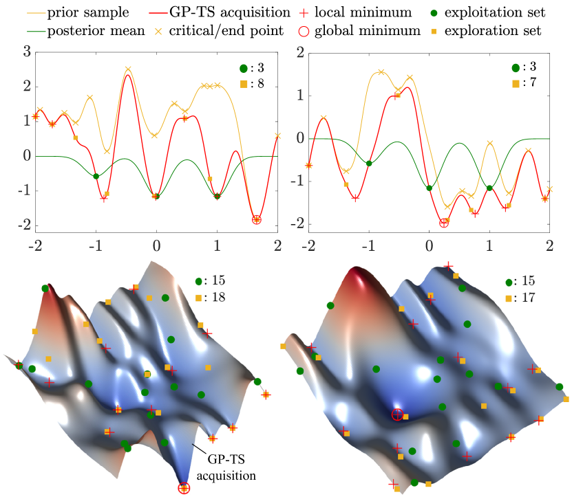
We define TS-roots as a global optimization algorithm for GP posterior samples (given the assumptions) via gradient-based multistart optimization, where the starting points include a subset of the local minima of a corresponding prior sample, , and a subset of the observed locations, . We call the exploration set and the exploitation set. Let
| (3) |
be the smallest local minima of the prior sample and be the posterior mean function. The starting points are defined as:
| (4) |
Here, and are imposed to control the cost of gradient-based multistart optimization, and is set to limit the number of evaluations of in the determination of . Considering the cost difference, in general we can have .
3.2 Relations between the Local Minima of Prior and Posterior Samples
Figure 1 shows several posterior samples in one and two dimensions, each marked with its local minima and global minimum . Here the exploration set is the local minima of , and the exploitation set is the observed locations . We make the following observations:
-
(1)
The prior sample is more complex than the data adjustment in the sense that it is less smooth and has more critical points. The comparison of smoothness can be made rigorous in various ways: for example, for GPs with a Matérn covariance function where the smoothness parameter is finite, is almost everywhere one time less differentiable than (see e.g., Garnett [4] Sec. 10.2, Kanagawa et al. [32]).
-
(2)
Item (1) implies that when the prior sample is added to the smoother landscape of , each local minimum of will be located near a local minimum of the posterior sample . Away from the observed locations , each is closely associated with an , with minimal change in location. In the vicinity of , an may have both a data point and an nearby, but because of the smoothness difference of and , in most cases the one closest to is an .
-
(3)
It is possible that near , sharp changes in may require sharp adjustments to the data, which may move some by a significant distance, or create new that are not near any or any .
-
(4)
Searching from with good observed values can discover good in the vicinity of , which can pick up some local minima not readily discovered by . This is especially true if is relatively flat near .
-
(5)
Since the posterior sample adapts to the data set, searches from will tend to converge to a good among all the local optima near . Even if the searches from cannot discover all the local minima in its vicinity, they tend to discover a good subset of them. Therefore, (4) can help address the issue in (3), if not fully eliminating it. By combining subsets of and , we can expect that the set of local minima of discovered with these starting points includes the global minimum with a high probability with respect to .
3.3 Representation of Prior Sample Local Minima
For each component function of the prior sample , define , , and for . We call a coordinate of mono type if and call it of mixed type if . Let be the set of interior critical points of such that and , . Denote and . Partition the set of candidate coordinates into mono type and mixed type . Proposition 1 gives a representation of the sets of strong local extrema of the prior sample. Its proof and the set sizes therein are given in Appendix A.
Proposition 1.
The set of strong local minima of the prior sample can be written as:
| (5) |
where tensor grids , . The set of strong local maxima of has an analogous representation, and satisfies , where is the disjoint union.
Critical Points of Univariate Functions via Global Rootfinding.
To compute the set of all critical points of is to compute all the roots of the derivative on the interval . Since is continuous, this can be solved robustly and efficiently by approximating the function with a Chebyshev or Legendre polynomial and solving a structured eigenvalue problem (see e.g., Trefethen [33]). The roots algorithm for global rootfinding based on polynomial approximation is given as Algorithm 2 in Appendix C.
3.4 Ordering of Prior Sample Local Minima
While the size of grows exponentially in domain dimension , its representation in Eq. 5 enables an efficient algorithm to compute the best subset (eq. 3) without enumerating its elements. With Eq. 5, we see that consists of all the local minima of with negative function values. Consider the case where has at least elements so that in the definition of we can replace with , which in turn can be replaced with . As we will show later, the problem of finding the largest elements of within is easier than finding the smallest negative elements of . Once the former is solved, we can solve the latter simply by removing the positive elements. Therefore, we convert the problem of Eq. 3 into three steps:
-
1.
, with buffer coefficient ;
-
2.
, so that ;
-
3.
, assuming that .
The last two steps are by enumeration and straightforward. The first step can be solved efficiently using min-heaps, with a time complexity that scales linearly in rather than , see Appendix B. The coefficient is chosen so that . The case when can be handled similarly. If , no subsetting is needed. The overall procedure to compute is given in Algorithm 3 in Appendix C.
4 Related Works
Sampling from Gaussian Process Posteriors.
A prevalent method to sample GP posteriors with stationary covariance functions is via weight-space approximations based on Bayesian linear models of random Fourier features [34]. This method, unfortunately, is subject to the variance starvation problem [16, 30] which can be mitigated using more accurate feature representations (see e.g., [35, 36]). An alternative is pathwise conditioning [30] that draws GP posterior samples by updating the corresponding prior samples. The decoupled representation of the pathwise conditioning can be further reformulated as two stochastic optimization problems for the posterior mean and an uncertainty reduction term, which are then efficiently solved using stochastic gradient descent [37].
Optimization of Acquisition Functions.
While their global optima guarantee the Bayes’ decision rule, BO acquisition functions are highly non-convex and difficult to optimize [9]. Nevertheless, less attention has been given to the development of robust algorithms for optimizing these acquisition functions. For this inner-loop optimization, gradient-based optimizers are often selected because of their fast convergence and robust performance [38]. The implementation of such optimizers is facilitated by Monte Carlo (MC) acquisition functions whose derivatives are easy to evaluate [9]. Gradient-based optimizers also allow multistart settings that use a set of starting points which can be, for example, midpoints of data points [39], uniformly distributed samples over the input variable space [3, 40], or random points from a Latin hypercube design [41]. However, multistart-based methods with random search may have difficulty determining the non-flat regions of acquisition functions, especially in high dimensions [10].
Posterior Sample-Based Acquisition Functions.
As discussed in Section 1, the family of posterior sample-based acquisition functions is determined from samples of the posterior. GP-TS [8] is a notable member that extends the classical TS for finite-armed bandits to continuous settings of BO (see algorithms in Appendix D). GP-TS prefers exploration by the mechanism that iteratively samples a function from the GP posterior of the objective function, optimizes this function, and selects the resulting solution as the next candidate for objective evaluation. To further improve the exploitation of GP-TS, the sample mean of MC acquisition functions can be defined from multiple samples of the posterior [9, 27]. Different types of MC acquisition functions can also be used to inject beliefs about functions into the prior [42].
5 Results
We assess the performance of TS-roots in optimizing benchmark functions. We then compare the quality of solutions to the inner-loop optimization of GP-TS acquisition functions obtained from our proposed method, a gradient-based multistart optimizer with uniformly random starting points, and a genetic algorithm. We also show how TS-roots can improve the performance of MES. Finally, we propose a new sample-average posterior function and show how it affects the performance of GP-TS. The experimental details for the presented results are in Appendix F.
Optimizing Benchmark Functions.
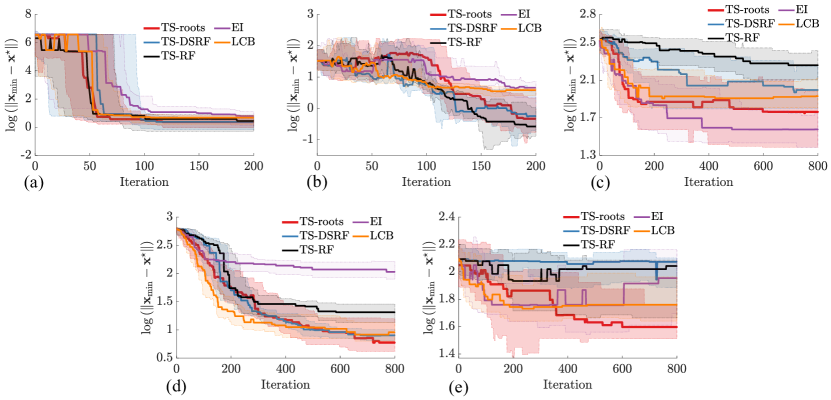
We test the empirical performance of TS-roots on challenging minimization problems of five benchmark functions: the 2D Schwefel, 4D Rosenbrock, 10D Levy, 16D Ackley, and 16D Powell functions [43]. The analytical expressions for these functions and their global minimum are given in Appendix E.
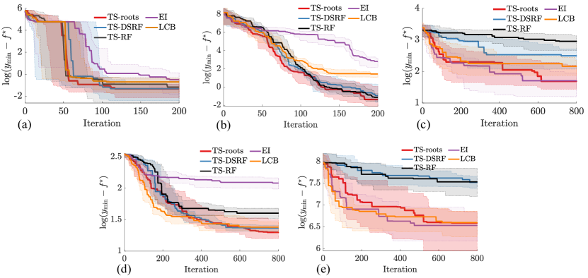
In each optimization iteration, we record the best observed value of the error and the distance , where , , , and are the best observation of the objective function in each iteration, the corresponding location of the observation, the true minimum value of the objective function, and the true minimum location, respectively. We compare the optimization results obtained from TS-roots and other BO methods, including GP-TS using decoupling sampling with random Fourier features (TS-DSRF), GP-TS with random Fourier features (TS-RF), expected improvement (EI) [1], and lower confidence bound (LCB)—the version of GP-UCB [5] for minimization problems.
Figure 2 shows the medians and interquartile ranges of solution values obtained from 20 runs of each of the considered BO methods. The corresponding histories of solution locations are in Figure 7 of Appendix G. With a fair comparison of outer-loop results (detailed in Appendix F), TS-roots surprisingly shows the best performance on the 2D Schwefel, 16D Ackley, and 16D Powell functions, and gives competitive results in the 4D Rosenbrock and 10D Levy problems. Notably, TS-roots recommends better solutions than its counterparts, TS-DSRF and TS-RF, in high-dimensional problems and offers competitive performance in low-dimensional problems. Across all the examples, EI and LCB tend to perform better in the initial stages, while TS-roots shows fast improvement in later stages. This is because GP-TS favors exploration, which delays rewards. The exploration phase, in general, takes longer for higher-dimensional problems.
Optimizing GP-TS Acquisition Functions via Rootfinding.
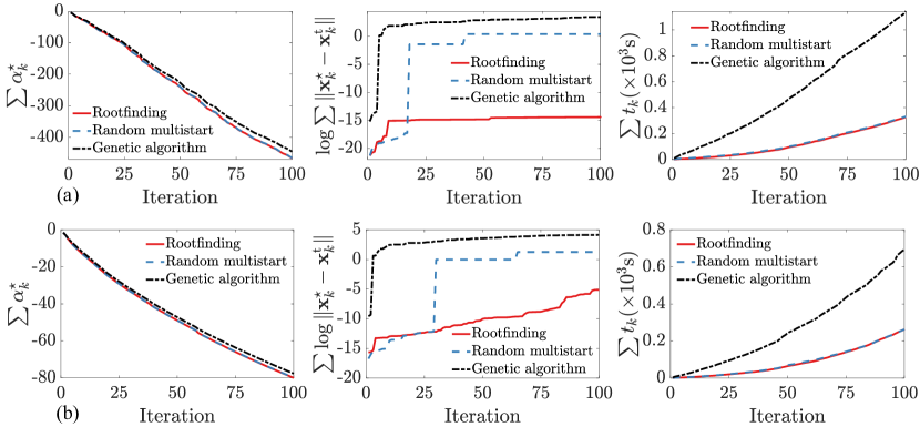
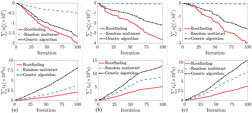
We assess the quality of solutions and computational cost for the inner-loop optimization of GP-TS acquisition functions by the proposed global optimization algorithm, termed rootfinding hereafter. We do so by computing the optimized values of the GP-TS acquisition functions, the corresponding solution points , and the CPU times required for optimizing the acquisition functions during the optimization process. For low-dimensional problems of the 2D Schwefel and 4D Rosenbrock functions, we also compute the exact global solution points of the GP-TS acquisition functions by starting the gradient-based optimizer at a large number of initial points (set as ), which is much greater than the maximum possible number of starting points set for TS-roots. For comparison, we extend the same GP-TS acquisition functions to inner-loop optimization using a gradient-based multistart optimizer with random starting points (i.e., random multistart) and a genetic algorithm. In each outer-loop optimization iteration, the number of starting points for the random multistart and the population size of the genetic algorithm are equal to the number of starting points recommended for rootfinding. The same termination conditions are used for the three algorithms.
Figure 3 shows the comparative performance of the inner-loop optimization for low-dimensional cases: the 2D Schwefel and 4D Rosenbrock functions. We see that the optimized acquisition function values and the optimization runtimes by rootfinding and the random multistart algorithm are almost identical, both of which are much better than those by the genetic algorithm. Rootfinding gives the best quality of the new solution points in both cases, while the genetic algorithm gives the worst. Notably in higher-dimensional settings of the 10D Levy, 16D Ackley, and 16D Powell functions shown in Figure 4, rootfinding performs much better than the random multistart and genetic algorithm in terms of optimized acquisition values and optimization runtimes, which verifies the importance of the judicious selection of starting points for global optimization of the GP-TS acquisition functions and the efficiency of rootfinding in high dimensions. The random multistart becomes worse in high dimensions.
TS-roots to Information-Theoretic Acquisition Functions.
We show how TS-roots can enhance the performance of MES [12], which uses information about the maximum function value for processing BO. One approach to computing MES generates a set of GP posterior samples using TS-RF and subsequently optimizes the generated functions for samples of using a gradient-based multistart optimizer with a large number of random starting points [12]. We hypothesize that high-quality samples can improve the performance of MES. Thus, we assign both TS-roots and TS-RF as the inner workings of MES and then compare the resulting optimal solutions.
Specifically, we minimize the 4D Rosenbrock, 6d Hartmann, and 10D Levy functions using four versions of MES, namely MES-R 10, MES-R 50, MES-TS-roots 10, and MES-TS-roots 50. Here, MES-R [12] and MES-TS-roots correspond to TS-RF and TS-roots, respectively, while 10 and 50 represent the number of random samples generated for computing the MES acquisition function in each iteration.
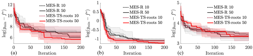
Figure 5 shows the optimization histories for ten independent runs of each MES method. On the 4D Rosenbrock and 6d Hartmann functions, MES with TS-roots demonstrates superior optimization performance and faster convergence compared to MES with TS-RF, especially when 50 samples of are generated. For the 10D Levy function, TS-roots outperforms TS-RF when using 10 samples of , while their performances are comparable when 50 samples are used.
Sample-Average Posterior Function.
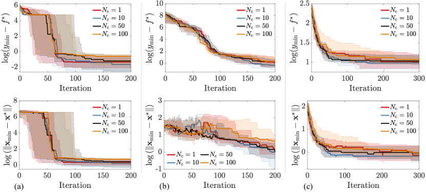
We finally propose a sample-average posterior function that explicitly controls exploration-exploitation balance and, notably, can be generated at the cost of generating one posterior sample. For noiseless observations with , we can rewrite the GP posterior function in Eq. 2 as , where . Define as the sample-average posterior function, where are samples generated from the GP posterior and . Since is deterministic, and the scaled prior sample can be written as , we have , where the first and second terms favor exploitation and exploration, respectively. Thus, we can consider an exploration-exploitation control parameter that, at large values, prioritizes exploitation by concentrating the conditional distribution of the global minimum location, i.e., , at the minimum location of , see Figure 8 in LABEL:{apd:AdditionalResults}. With , we can reproduce and the GP mean function by setting and , respectively.
We investigate how influences the outer-loop optimization results. For this, we set for TS-roots to optimize the 2D Schwefel, 4D Rosenbrock, and 6d Ackley functions. We observe that increasing from to improves TS-roots performance on the 2D Schwefel, 4D Rosenbrock, and 6d Ackley functions (see Figure 9 in Appendix G). However, further increases in from 10 to 50 and 100 result in slight declines in solution quality as TS-roots transitions to exploitation. These observations indicate that there is an optimal value of for each problem at which TS-roots achieves its best performance by balancing exploitation and exploration. However, identifying such an optimal value to maximize the performance of for a particular optimization problem is an open issue.
6 Conclusion and Future Work
We presented TS-roots, a global optimization strategy for posterior sample paths. It comprises an adaptive selection of starting points for gradient-based multistart optimizers, combining exploration with exploitation. This strategy breaks the curse of dimensionality by exploiting the separability of Gaussian process priors. Compared to random multistart and a genetic algorithm, TS-roots consistently yields higher-quality solutions in optimizing posterior sample-based acquisition functions for Bayesian optimization, both in low- and high-dimensional settings. It also improves the outer-loop optimization performance of GP-TS and information-theoretic acquisition functions such as MES. For future work, we extend TS-roots to other spectral representations per Bochner’s theorem [16, 35, 36]. We also plan to study the modes and the probability when TS-roots fails to find the global optimum, and the impact of subset sizes.
References
- Jones et al. [1998] Donald R. Jones, Matthias Schonlau, and William J. Welch. Efficient global optimization of expensive black-box functions. Journal of Global Optimization, 13(4):455–492, 1998. ISSN 1573-2916. doi:10.1023/A:1008306431147. URL https://doi.org/10.1023/A:1008306431147.
- Snoek et al. [2012] Jasper Snoek, Hugo Larochelle, and Ryan P Adams. Practical Bayesian optimization of machine learning algorithms. In F. Pereira, C.J. Burges, L. Bottou, and K.Q. Weinberger, editors, Advances in Neural Information Processing Systems, volume 25, pages 2951–2959. Curran Associates, Inc., 2012. URL https://proceedings.neurips.cc/paper_files/paper/2012/file/05311655a15b75fab86956663e1819cd-Paper.pdf.
- Frazier [2018] Peter I. Frazier. Bayesian optimization. In Esma Gel and Lewis Ntaimo, editors, Recent Advances in Optimization and Modeling of Contemporary Problems, INFORMS TutORials in Operations Research, chapter 11, pages 255–278. INFORMS, October 2018. ISBN 978-0-9906153-2-3. doi:10.1287/educ.2018.0188.
- Garnett [2023] Roman Garnett. Bayesian Optimization. Cambridge University Press, Cambridge, UK, 2023. doi:10.1017/9781108348973.
- Srinivas et al. [2010] Niranjan Srinivas, Andreas Krause, Sham M. Kakade, and Matthias Seeger. Gaussian process optimization in the bandit setting: No regret and experimental design. In Johannes Fürnkranz and Thorsten Joachims, editors, Proceedings of the 27th International Conference on Machine Learning, volume 13, pages 1015–1022. Omnipress, 2010. URL https://icml.cc/Conferences/2010/papers/422.pdf.
- Bull [2011] Adam D. Bull. Convergence rates of efficient global optimization algorithms. Journal of Machine Learning Research, 12(88):2879–2904, 2011. URL http://jmlr.org/papers/v12/bull11a.html.
- Russo and Van Roy [2014] Daniel Russo and Benjamin Van Roy. Learning to optimize via posterior sampling. Mathematics of Operations Research, 39(4):1221–1243, April 2014. ISSN 0364-765X. doi:10.1287/moor.2014.0650.
- Chowdhury and Gopalan [2017] Sayak Ray Chowdhury and Aditya Gopalan. On kernelized multi-armed bandits. In Doina Precup and Yee Whye Teh, editors, Proceedings of the 34th International Conference on Machine Learning, volume 70 of Proceedings of Machine Learning Research, pages 844–853. PMLR, 06–11 Aug 2017. URL https://proceedings.mlr.press/v70/chowdhury17a.html.
- Wilson et al. [2018] James Wilson, Frank Hutter, and Marc Deisenroth. Maximizing acquisition functions for Bayesian optimization. In S. Bengio, H. Wallach, H. Larochelle, K. Grauman, N. Cesa-Bianchi, and R. Garnett, editors, Advances in Neural Information Processing Systems, volume 31, pages 9884–9895. Curran Associates, Inc., 2018. URL https://proceedings.neurips.cc/paper/2018/hash/498f2c21688f6451d9f5fd09d53edda7-Abstract.html.
- Rana et al. [2017] Santu Rana, Cheng Li, Sunil Gupta, Vu Nguyen, and Svetha Venkatesh. High dimensional Bayesian optimization with elastic Gaussian process. In Doina Precup and Yee Whye Teh, editors, Proceedings of the 34th International Conference on Machine Learning, volume 70, pages 2883–2891. PMLR, 06–11 Aug 2017. URL https://proceedings.mlr.press/v70/rana17a.html.
- Hernández-Lobato et al. [2014] José Miguel Hernández-Lobato, Matthew W. Hoffman, and Zoubin Ghahramani. Predictive entropy search for efficient global optimization of black-box functions. In Z. Ghahramani, M. Welling, C. Cortes, N. Lawrence, and K.Q. Weinberger, editors, Advances in Neural Information Processing Systems, volume 27, pages 918–926. Curran Associates, Inc., 2014. URL https://proceedings.neurips.cc/paper_files/paper/2014/hash/069d3bb002acd8d7dd095917f9efe4cb-Abstract.html.
- Wang and Jegelka [2017] Zi Wang and Stefanie Jegelka. Max-value entropy search for efficient Bayesian optimization. In Doina Precup and Yee Whye Teh, editors, Proceedings of the 34th International Conference on Machine Learning, volume 70, pages 3627–3635. PMLR, 2017. URL https://proceedings.mlr.press/v70/wang17e.html.
- Hvarfner et al. [2022] Carl Hvarfner, Frank Hutter, and Luigi Nardi. Joint entropy search for maximally-informed Bayesian optimization. In S. Koyejo, S. Mohamed, A. Agarwal, D. Belgrave, K. Cho, and A. Oh, editors, Advances in Neural Information Processing Systems, volume 35, pages 11494–11506. Curran Associates, Inc., 2022. URL https://proceedings.neurips.cc/paper_files/paper/2022/file/4b03821747e89ce803b2dac590f6a39b-Paper-Conference.pdf.
- Tu et al. [2022] Ben Tu, Axel Gandy, Nikolas Kantas, and Behrang Shafei. Joint entropy search for multi-objective bayesian optimization. In S. Koyejo, S. Mohamed, A. Agarwal, D. Belgrave, K. Cho, and A. Oh, editors, Advances in Neural Information Processing Systems, volume 35, pages 9922–9938. Curran Associates, Inc., 2022. URL https://proceedings.neurips.cc/paper_files/paper/2022/file/4086fe59dc3584708468fba0e459f6a7-Paper-Conference.pdf.
- Russo and Van Roy [2016] Daniel J. Russo and Benjamin Van Roy. An information-theoretic analysis of Thompson sampling. The Journal of Machine Learning Research, 17(1):2442–2471, 2016. ISSN 1532-4435. URL https://www.jmlr.org/papers/v17/14-087.html.
- Mutny and Krause [2018] Mojmir Mutny and Andreas Krause. Efficient high dimensional Bayesian optimization with additivity and quadrature Fourier features. In S. Bengio, H. Wallach, H. Larochelle, K. Grauman, N. Cesa-Bianchi, and R. Garnett, editors, Advances in Neural Information Processing Systems, volume 31, pages 9005–9016. Curran Associates, Inc., 2018. URL https://proceedings.neurips.cc/paper/2018/hash/4e5046fc8d6a97d18a5f54beaed54dea-Abstract.html.
- MacKay [2003] David J. C. MacKay. Information theory, inference, and learning algorithms. Cambridge University Press, Cambridge, UK, 2003. URL https://www.cambridge.org/9780521642989.
- Shah and Ghahramani [2015] Amar Shah and Zoubin Ghahramani. Parallel predictive entropy search for batch global optimization of expensive objective functions. In C. Cortes, N. Lawrence, D. Lee, M. Sugiyama, and R. Garnett, editors, Advances in Neural Information Processing Systems, volume 28. Curran Associates, Inc., 2015. URL https://proceedings.neurips.cc/paper_files/paper/2015/file/57c0531e13f40b91b3b0f1a30b529a1d-Paper.pdf.
- Hernández-Lobato et al. [2017] José Miguel Hernández-Lobato, James Requeima, Edward O. Pyzer-Knapp, and Alán Aspuru-Guzik. Parallel and distributed Thompson sampling for large-scale accelerated exploration of chemical space. In Doina Precup and Yee Whye Teh, editors, Proceedings of the 34th International Conference on Machine Learning, volume 70 of Proceedings of Machine Learning Research, pages 1470–1479. PMLR, 06–11 Aug 2017. URL https://proceedings.mlr.press/v70/hernandez-lobato17a.html.
- Kandasamy et al. [2018] Kirthevasan Kandasamy, Akshay Krishnamurthy, Jeff Schneider, and Barnabas Poczos. Parallelised Bayesian optimisation via Thompson sampling. In Amos Storkey and Fernando Perez-Cruz, editors, Proceedings of the Twenty-First International Conference on Artificial Intelligence and Statistics, volume 84 of Proceedings of Machine Learning Research, pages 133–142. PMLR, 09–11 Apr 2018. URL https://proceedings.mlr.press/v84/kandasamy18a.html.
- Kushner [1964] Harold J. Kushner. A new method of locating the maximum point of an arbitrary multipeak curve in the presence of noise. Journal Basic Engineering, 86(1):97–106, 1964. doi:10.1115/1.3653121.
- Jones et al. [1993] D. R. Jones, C. D. Perttunen, and B. E. Stuckman. Lipschitzian optimization without the Lipschitz constant. Journal of Optimization Theory and Applications, 79(1):157–181, 1993. ISSN 1573-2878. doi:10.1007/BF00941892. URL https://doi.org/10.1007/BF00941892.
- Hansen et al. [2003] Nikolaus Hansen, Sibylle D. Müller, and Petros Koumoutsakos. Reducing the time complexity of the derandomized evolution strategy with covariance matrix adaptation (CMA-ES). Evolutionary Computation, 11(1):1–18, 2003. doi:10.1162/106365603321828970.
- Mitchell [1998] Melanie Mitchell. An introduction to genetic algorithms. The MIT Press, Massachusetts, USA, 1998.
- Kim and Choi [2021] Jungtaek Kim and Seungjin Choi. On local optimizers of acquisition functions in Bayesian optimization. In Frank Hutter, Kristian Kersting, Jefrey Lijffijt, and Isabel Valera, editors, Machine Learning and Knowledge Discovery in Databases, pages 675–690, Cham, 2021. Springer International Publishing. doi:10.1007/978-3-030-67661-2_40.
- Bergstra and Bengio [2012] James Bergstra and Yoshua Bengio. Random search for hyper-parameter optimization. Journal of Machine Learning Research, 13(10):281–305, 2012. URL http://jmlr.org/papers/v13/bergstra12a.html.
- Balandat et al. [2020] Maximilian Balandat, Brian Karrer, Daniel Jiang, Samuel Daulton, Ben Letham, Andrew G Wilson, and Eytan Bakshy. BoTorch: A framework for efficient Monte-Carlo Bayesian optimization. In Advances in Neural Information Processing Systems, volume 33, pages 21524–21538. Curran Associates, Inc., 2020. URL https://proceedings.neurips.cc/paper_files/paper/2020/file/f5b1b89d98b7286673128a5fb112cb9a-Paper.pdf.
- Feo and Resende [1995] Thomas A. Feo and Mauricio G. C. Resende. Greedy randomized adaptive search procedures. Journal of Global Optimization, 6(2):109–133, 1995. ISSN 1573-2916. doi:10.1007/BF01096763. URL https://doi.org/10.1007/BF01096763.
- Chapelle and Li [2011] Olivier Chapelle and Lihong Li. An empirical evaluation of Thompson sampling. In J. Shawe-Taylor, R. Zemel, P. Bartlett, F. Pereira, and K.Q. Weinberger, editors, Advances in Neural Information Processing Systems, volume 24, pages 2249–2257. Curran Associates, Inc., 2011. URL https://papers.nips.cc/paper_files/paper/2011/hash/e53a0a2978c28872a4505bdb51db06dc-Abstract.html.
- Wilson et al. [2020] James Wilson, Viacheslav Borovitskiy, Alexander Terenin, Peter Mostowsky, and Marc Deisenroth. Efficiently sampling functions from Gaussian process posteriors. In Hal Daumé III and Aarti Singh, editors, Proceedings of the 37th International Conference on Machine Learning, volume 119 of Proceedings of Machine Learning Research, pages 10292–10302. PMLR, 13–18 Jul 2020. URL https://proceedings.mlr.press/v119/wilson20a.html. GitHub repo: https://github.com/j-wilson/GPflowSampling.
- Duvenaud et al. [2013] David Duvenaud, James Lloyd, Roger Grosse, Joshua Tenenbaum, and Ghahramani Zoubin. Structure discovery in nonparametric regression through compositional kernel search. In Proceedings of the 30th International Conference on Machine Learning, volume 28, pages 1166–1174, Atlanta, Georgia, USA, 2013. URL http://proceedings.mlr.press/v28/duvenaud13.html.
- Kanagawa et al. [2018] Motonobu Kanagawa, Philipp Hennig, Dino Sejdinovic, and Bharath K Sriperumbudur. Gaussian processes and kernel methods: A review on connections and equivalences, 2018. URL https://arxiv.org/abs/1807.02582.
- Trefethen [2019] Lloyd N. Trefethen. Approximation Theory and Approximation Practice, Extended Edition, volume 164 of Other Titles in Applied Mathematics. Society for Industrial and Applied Mathematics, Philadelphia, PA, 2019. ISBN 978-1-61197-593-2. doi:10.1137/1.9781611975949. URL https://people.maths.ox.ac.uk/trefethen/ATAP/. First edition, 2013; Extended edition, 2019.
- Rahimi and Recht [2007] Ali Rahimi and Benjamin Recht. Random features for large-scale kernel machines. In J. Platt, D. Koller, Y. Singer, and S. Roweis, editors, Advances in Neural Information Processing Systems, volume 20, pages 1177–1184. Curran Associates, Inc., 2007. URL https://proceedings.neurips.cc/paper_files/paper/2007/file/013a006f03dbc5392effeb8f18fda755-Paper.pdf.
- Hensman et al. [2018] James Hensman, Nicolas Durrande, and Arno Solin. Variational Fourier features for Gaussian processes. Journal of Machine Learning Research, 18(151):1–52, 2018. URL http://jmlr.org/papers/v18/16-579.html.
- Solin and Särkkä [2020] Arno Solin and Simo Särkkä. Hilbert space methods for reduced-rank Gaussian process regression. Statistics and Computing, 30(2):419–446, 2020. ISSN 1573-1375. doi:10.1007/s11222-019-09886-w.
- Lin et al. [2023] Jihao Andreas Lin, Javier Antorán, Shreyas Padhy, David Janz, José Miguel Hernández-Lobato, and Alexander Terenin. Sampling from Gaussian process posteriors using stochastic gradient descent. In A. Oh, T. Naumann, A. Globerson, K. Saenko, M. Hardt, and S. Levine, editors, Advances in Neural Information Processing Systems, volume 36, pages 36886–36912. Curran Associates, Inc., 2023. URL https://proceedings.neurips.cc/paper_files/paper/2023/file/7482e8ce4139df1a2d8195a0746fa713-Paper-Conference.pdf.
- Daulton et al. [2020] Samuel Daulton, Maximilian Balandat, and Eytan Bakshy. Differentiable expected hypervolume improvement for parallel multi-objective bayesian optimization. In H. Larochelle, M. Ranzato, R. Hadsell, M.F. Balcan, and H. Lin, editors, Advances in Neural Information Processing Systems, volume 33, pages 9851–9864. Curran Associates, Inc., 2020. URL https://proceedings.neurips.cc/paper_files/paper/2020/file/6fec24eac8f18ed793f5eaad3dd7977c-Paper.pdf.
- Jones [2001] Donald R. Jones. A taxonomy of global optimization methods based on response surfaces. Journal of Global Optimization, 21(4):345–383, 2001. ISSN 1573-2916. doi:10.1023/A:1012771025575.
- Ament et al. [2023] Sebastian Ament, Samuel Daulton, David Eriksson, Maximilian Balandat, and Eytan Bakshy. Unexpected improvements to expected improvement for Bayesian optimization. In A. Oh, T. Naumann, A. Globerson, K. Saenko, M. Hardt, and S. Levine, editors, Advances in Neural Information Processing Systems, volume 36, pages 20577–20612. Curran Associates, Inc., 2023. URL https://proceedings.neurips.cc/paper_files/paper/2023/file/419f72cbd568ad62183f8132a3605a2a-Paper-Conference.pdf.
- Wang et al. [2020] Jialei Wang, Scott C. Clark, Eric Liu, and Peter I. Frazier. Parallel Bayesian global optimization of expensive functions. Operations Research, 68(6):1850–1865, 2020. doi:10.1287/opre.2019.1966. URL https://doi.org/10.1287/opre.2019.1966.
- Hvarfner et al. [2024] Carl Hvarfner, Frank Hutter, and Luigi Nardi. A general framework for user-guided bayesian optimization. In The Twelfth International Conference on Learning Representations, pages 9851–9864. ICLR 2024, 2024. URL https://iclr.cc/virtual/2024/poster/18774.
- Surjanovic and Bingham [2013] S Surjanovic and D Bingham. Virtual library of simulation experiments: Test functions and datasets, 2013. URL http://www.sfu.ca/~ssurjano/optimization.html.
- Rasmussen and Williams [2006] Carl Edward Rasmussen and Christopher K I Williams. Gaussian processes for machine learning. The MIT Press, Massachusetts, USA, 2006. ISBN 9780521872508. doi:10.7551/mitpress/3206.001.0001. URL https://doi.org/10.7551/mitpress/3206.001.0001.
- Zhu et al. [1998] Huaiyu Zhu, C. K. I Williams, R Rohwer, and M Morciniec. Gaussian regression and optimal finite dimensional linear models. In Christopher M Bishop, editor, Neural Networks and Machine Learning, 1998. URL https://publications.aston.ac.uk/id/eprint/38366/.
- Gradshteyn and Ryzhik [2014] I.S. Gradshteyn and I.M. Ryzhik. Table of Integrals, Series, and Products. Academic Press, Boston, 8th edition, 2014. ISBN 978-0-12-384933-5. doi:10.1016/C2010-0-64839-5.
- Battles and Trefethen [2004] Zachary Battles and Lloyd N. Trefethen. An extension of MATLAB to continuous functions and operators. SIAM Journal on Scientific Computing, 25(5):1743–1770, 2004. doi:10.1137/S1064827503430126. URL https://doi.org/10.1137/S1064827503430126.
- Richardson [2016] Mark Richardson. chebpy, a Python implementation of chebfun, 2016. URL https://github.com/chebpy/chebpy.
- Picheny et al. [2013] Victor Picheny, Tobias Wagner, and David Ginsbourger. A benchmark of kriging-based infill criteria for noisy optimization. Structural and multidisciplinary optimization, 48:607–626, 2013. doi:10.1007/s00158-013-0919-4. URL https://doi.org/10.1007/s00158-013-0919-4.
- Owen [1992] Art B. Owen. A Central Limit Theorem for Latin Hypercube Sampling. Journal of the Royal Statistical Society: Series B (Methodological), 54(2):541–551, 12 1992. ISSN 0035-9246. doi:10.1111/j.2517-6161.1992.tb01895.x. URL https://doi.org/10.1111/j.2517-6161.1992.tb01895.x.
Appendix A Characterizing the Local Minima of a Separable Function
A.1 Proof of Proposition 1: A Representation of the Set of Local Minima
Proposition 1 broadly applies to separable functions on a hypercube. Consider a separable function with domain , where . To simplify the discussion, we further assume that is twice differentiable at its interior critical points . The gradient of can be written as:
| (6) |
where . The Hessian of can be written as:
| (7) |
where .
An interior point is a strong local minimum of if and only if and . From Eq. 6, the first condition is satisfied in any of the following three cases: (1) and for all ; (2) for exactly one and ; or (3) for all where .
In case (1), the Hessian Eq. 7 reduces to , which is positive definite if and only if one of the following holds: (i) and , for all ; or (ii) and , for all .
In case (2), the Hessian reduces to an all-zero matrix except for the th diagonal entry: . Even if this entry is positive, the Hessian is still positive semi-definite, which means that there is a continuum of weak local minima: . Besides, this case requires and to have an identical root, which an event with probability zero.
In case (3), let be a shifted version of , . Taylor expansion at gives for all and for all . We have , where . This means that there is a continuum of saddle points: .
For a boundary point , we partition the index set into , and such that for all , for all , and for all . Define for any subset of the indices. Then is a strong local minimum of if and only if the following conditions hold: (a) is a strong local minimum in ; (b) ; and (c) .
Condition (a) holds if any only if and . Based on the previous discussion on interior local minima, it is equivalent to: (i) and , for all ; or (ii) and , for all .
Similarly, condition (c) is equivalent to: (i) and , for all ; or (ii) and , for all .
Summarizing the above discussions, we see that there is a unified way to identify the set of all strong local minima of , which is stated in Proposition 1. The discussion for the set of local maxima is the exactly the same, except that the signs are flipped. This also means that and form a partition of the union of the two tensor grids.
If is not twice differentiable at some interior critical point , we may replace with the statement that is a strong local minimum of , and replace with the statement that is a strong local maximum of . The rest of the discussion still follows. In practice, the differentiability of the prior sample is not an issue, because it is almost always approximated by a finite sum of analytic functions, which is again analytic.
A.2 Number of Local Minima of a Separable Function
In Proposition 1, each set of candidate coordinates is partitioned into mono type and mixed type:
Another partition of is by the sign of the corresponding component function value:
These two partitions create a finer partition of into four subsets:
Denote the sizes of mixed and mono type candidate coordinates as and , then the sizes of the two tensor grids and can be written as:
Define signed sums as the sums of signs of function values on the two tensor grids:
We now derive efficient formulas to calculate these signed sums, using as an example. Denote each coordinate in as . Denote each point in as , where multi-index . The signed sum can be written as:
A formula for can be derived analogously. Denote set sizes:
then the signed sums can be calculated as:
The sizes of negative and positive strong local minima of a separable function can be written as:
| (8) | |||
Therefore, the size of the strong local minima of a separable function can be written as:
| (9) |
Appendix B Ordering the Local Minima of a Separable Function
B.1 Filtering a Tensor Grid for High Absolute Values of a Separable Function
The step one in Section 3.4 is equivalent to the following problem: given coordinates and components values , , of a separable function , find points such that are the largest in the tensor grid .
Because , we can solve this problem as follows: define two-dimensional arrays and , solve , and return . Here the maxk_sum algorithms finds the combinations from that gives the largest sums, which is described next.
B.2 Top Combinations with the Largest Sums
Consider this problem: given a two-dimensional array , , with , , find multi-indices of the form such that the sums are the largest among all combinations .
An exhaustive search is intractable because the number of all possible combinations grows exponentially as . Instead, we use a min-heap to efficiently keep track of the top combinations. A min-heap is a complete binary tree, where each node is no greater than its children. The operations of inserting an element and removing the smallest element from a min-heap can be done in logarithmic time. Algorithm 1 gives a procedure to solve the above problem using min-heaps.
This algorithm has time complexity , where , and space complexity . In TS-roots, the cost of maxk_sum is small compared with the gradient-based multistart optimization of the posterior sample.
Appendix C Algorithms for TS-roots
C.1 Spectral Sampling of Separable Gaussian Process Priors
Per Mercer’s theorem on probability spaces (see e.g., [44], Sec 4.3), any positive definite covariance function that is essentially bounded with respect to some probability measure on a compact domain has a spectral representation , where is a pair of eigenvalue and eigenfunction of the kernel integral operator. The corresponding GP prior can be written as , where are independent standard Gaussian random variables. Similar spectral representations exist per Bochner’s theorem, which may have efficient discretizations [36, 16].
Given spectral representations of the univariate component functions of a separable Gaussian Process prior, we can accurately approximate the prior sample as
| (10) |
Here is selected for each variate such that , where is sufficiently small (see Appendix F for the value used in this study). Using spectral representations of the univariate components as in Eq. 10 is much more efficient than directly using a spectral representation of the separable GP prior, because the former uses univariate terms to exactly represent multivariate terms in the latter.
Spectrum of the Squared Exponential Covariance Function.
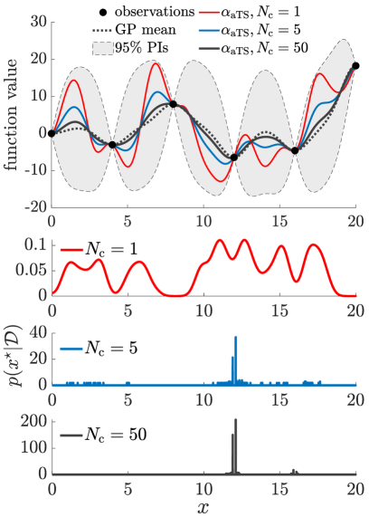
The univariate squared exponential (SE) covariance function can be written as , where the relative distance . The spectral representation of such a covariance function per Mercer’s theorem is . With a Gaussian measure over the domain , we can write the eigenvalues and eigenfunctions of the kernel integral operator as follows. (See e.g., [45] Sec. 4 and [46] 7.374 eq. 8.)
Define constants , , , and . For , the th eigenvalue is and the corresponding eigenfunction is , where and the th-order Hermite polynomial defined by .
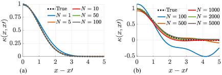
Figure 6 shows approximations to the SE covariance function by truncated spectral representations with the first eigenpairs and by random Fourier features [34] with basis functions. The spectral representation per Mercer’s theorem converges quickly to the true covariance function, while the random Fourier features representation requires a large number of basis functions and is inaccurate for .
C.2 Univariate Global Rootfinding
Algorithm 2 outlines a method for univariate global rootfinding on an interval by solving an eigenvalue problem. When the orthogonal polynomial basis is the Chebyshev polynomials, the corresponding comrade matrix is called a colleague matrix, and we have the following theorem:
(or approximate on the interval using such a basis)
Theorem 1.
Let , , be a polynomial of degree , where is the th Chebyshev polynomial and is the corresponding weight. The roots of are the eigenvalues of the following colleague matrix:
| (11) |
where the elements not displayed are zero.
A proof of Theorem 1 is provided in [33], Chapter 18. A classical formula to compute the weights requires floating point operations, which can be reduced to using a fast Fourier transform. Since the colleague matrix is tridiagonal except in the final row, the complexity of computing its eigenvalues can be improved from to operations, which can be further improved to via recursive subdivision of intervals (see Trefethen [33]). The roots algorithm is implemented in the Chebfun package in MATLAB [47] and the chebpy package in Python [48]; both packages also implement other related programs such as chebfun for Chebyshev polynomial approximation and diff for differentiation.
Compute first and second derivatives
Include interval lower and upper bounds
Candidate coordinate values
, Univariate second derivatives at critical points
; Univariate inward derivatives at interval ends
Values at mono and mixed type candidate coordinates
Sizes of tensor grids
Signed sums
C.3 Best Local Minima of a Separable Function
Given the univariate component functions of a separable function, Algorithm 3 finds the subset of the local minima of the function with the smallest function values. This procedure requires the maxk_sum algorithm in Algorithm 1, the roots algorithm in Algorithm 2 and the related programs chebfun and diff, see also Appendix F.
In Algorithm 3, are two-dimensional arrays, while are matrices. Function evaluations at 10, 11, 15, 20, 21 and 25 are only notational: the sign and value of the function can be computed efficiently by multiplying the signs and values of its components at the selected coordinates. For example, the statement at 10 can be evaluated as , where is a two-dimensional array with , is a matrix with columns, and rowXor is row-wise exclusive or operation. Similarly, the statement at 11 can be evaluated as , where rowProd is row products.
C.4 Decoupled Sampling from Gaussian Process Posteriors
The decoupled sampling method for GP posteriors [30], together with the spectral sampling of separable GP priors, is outlined in Algorithm 4.
Appendix D Bayesian Optimization via Thompson Sampling
A general procedure for sequential optimization is given in Algorithm 5. The initial dataset can either be empty or contain some observations. In the latter case we can write , where . Three components of this algorithm can be customized: the observation model , the optimization policy , and the termination condition.
BO can be seen as an optimization policy for sequential optimization. A formal procedure is given in Algorithm 6. Three components of this algorithm can be customized: the prior probabilistic model , the acquisition function , and the global optimization algorithm. Any probabilistic model of the objective function can be seen as a probability distribution on a function space, and the prior is usually specified as a stochastic process such as a GP. The acquisition function derived from the posterior can be either deterministic—such as EI and LCB—or stochastic, such as GP-TS. To simplify notation, we state the global optimization problem of as minimization rather than maximization. The two problems are the same with a change of sign to the objective.
When applied to BO, GP-TS generates a random acquisition function simply by sampling the posterior model. That is, given the posterior at the th BO iteration, the GP-TS acquisition function is a random function: .
Appendix E Benchmark Functions
The analytical expressions for the benchmark functions used in Section 5 are given below. The global solutions of these functions are detailed in [43].
Schwefel Function:
| (12) |
This function is evaluated on and has a global minimum at . This function is at .
Rosenbrock Function:
| (13) |
This function is evaluated on and has a global minimum at .
Levy Function:
| (14) |
where , . This function is evaluated on and has a global minimum at .
Ackley Function:
| (15) |
where , , and . This function is evaluated on and has a global minimum at . This function not differentiable at .
Powell Function:
| (16) |
This function is evaluated on and has a global minimum at .
6d Hartmann Function:
| (17) |
where
| (18a) | |||
| (18b) | |||
| (18c) |
This function is evaluated on and has a global minimum at . The rescaled version [49] is used in the experiments.
Appendix F Experimental Details
Data Generation.
We generate 20 initial datasets for each problem. The input observations are randomly generated using the Latin hypercube sampling [50] within , where represents the number of input variables. The normalized input observations are transformed into their real spaces to evaluate the corresponding objective function values which are then standardized using the -score for processing optimization. Each BO method in comparison starts from each of the generated datasets.
Key Parameters for TS-roots and other BO Methods.
We use squared exponential (SE) covariance functions for our experiments. The spectra of univariate SE covariance functions for all problems (see Section C.1) are determined using the Gaussian measure . The number of terms , , of each truncated univariate spectrum is determined such that , where . If , we set to trade off between the accuracy of truncated spectra and computational cost. The maximum size of the exploration set is . The maximum size of the exploitation set is .
The number of initial observations is for all problems. The standard deviation of observation noise is applied for standardized output observations. The number of BO iterations for the 2D Schwefel and 4D Rosenbrock functions is 200, while that for the 10D Levy, 16D Ackley, and 16D Powell functions is 800. Other GP-TS methods for optimization of benchmark test functions including TS-DSRF (i.e., TS using decoupled sampling with random Fourier features) and TS-RF (i.e., TS using random Fourier features) are characterized by a total of 2000 random Fourier features.
To ensure a fair comparison of outer-optimization results, we first implement TS-roots and record the number of starting points used in each optimization iteration. We then apply other BO methods, each employing a gradient-based multistart optimizer with the same number of random starting points and identical termination criteria as those used for TS-roots in each iteration.
For the comparative inner-loop optimization performance of the proposed method via rootfinding with the random multistart and genetic algorithm approaches, we set the same termination tolerance on the objective function value as the stopping criterion for the methods. In addition, the number of starting points for the random multistart and the population size of the genetic algorithm are the same as the number of points in both the exploration and exploitation sets of rootfinding in each optimization iteration.
Computational Tools.
We carry out all experiments, except those for inner-loop optimization, using a designated cluster at our host institution. This cluster hosts 9984 Intel CPU cores and 327680 Nvidia GPU cores integrated within 188 compute and 20 GPU nodes. The inner-loop optimization is implemented on a PC with an Intel® CoreTM i7-1165G7 @ 2.80 GHz and 16 GB memory.
Appendix G Additional Results
Distance to Global Minimum.
Figure 7 shows the solution locations from 20 runs of TS-roots, TS-DSRF, TS-RF, EI, and LCB for the 2D Schwefel, 4D Rosenbrock, 10D Levy, 16D Ackley, 16D Powell functions.
Sample-average Posterior Function.
Figure 8 shows how we can improve the exploitation of GP-TS when increasing the exploration-exploitation control parameter .
Performance of Sample-average TS-roots.
Figure 9 shows the performance of sample-average TS-roots with different exploration-exploitation control parameters for the 2D Schwefel, 4D Rosenbrock, and 6d Ackley functions.