Online Detecting LLM-Generated Texts via Sequential Hypothesis Testing by Betting
Abstract
Developing algorithms to differentiate between machine-generated texts and human-written texts has garnered substantial attention in recent years. Existing methods in this direction typically concern an offline setting where a dataset containing a mix of real and machine-generated texts is given upfront, and the task is to determine whether each sample in the dataset is from a large language model (LLM) or a human. However, in many practical scenarios, sources such as news websites, social media accounts, or on other forums publish content in a streaming fashion. Therefore, in this online scenario, how to quickly and accurately determine whether the source is an LLM with strong statistical guarantees is crucial for these media or platforms to function effectively and prevent the spread of misinformation and other potential misuse of LLMs. To tackle the problem of online detection, we develop an algorithm based on the techniques of sequential hypothesis testing by betting that not only builds upon and complements existing offline detection techniques but also enjoys statistical guarantees, which include a controlled false positive rate and the expected time to correctly identify a source as an LLM. Experiments were conducted to demonstrate the effectiveness of our method.
1 Introduction
Over the past few years, there has been growing evidence that LLMs can produce content with qualities on par with human-level writing, including writing stories (Yuan et al., 2022), producing educational content(Kasneci et al., 2023), and summarizing news(Zhang et al., 2024). On the other hand, concerns about potentially harmful misuses have also accumulated in recent years, such as producing fake news(Zellers et al., 2019), misinformation(Lin et al., 2021; Chen and Shu, 2023), plagiarism(Bommasani et al., 2021; Lee et al., 2023), malicious product reviews(Adelani et al., 2020), and cheating(Stokel-Walker, 2022; Susnjak and McIntosh, 2024). To tackle the relevant issues associated with the rise of LLMs, a burgeoning body of research has been dedicated to distinguishing between human-written and machine-generated texts (Jawahar et al., 2020; Lavergne et al., 2008; Hashimoto et al., 2019; Gehrmann et al., 2019; Mitchell et al., 2023; Su et al., 2023; Bao et al., 2023; Solaiman et al., 2019; Bakhtin et al., 2019; Zellers et al., 2019; Ippolito et al., 2019; Tian, 2023; Uchendu et al., 2020; Fagni et al., 2021; Adelani et al., 2020; Abdelnabi and Fritz, 2021; Zhao et al., 2023; Kirchenbauer et al., 2023; Christ et al., 2024).
While these existing methods can efficiently identify a text source in an offline setting where all the texts to be classified are provided in a single shot, they are not specifically designed to handle scenarios where texts arrive sequentially, and therefore, they might not be directly applicable to the online setting, where certain serious challenges have been observed over the past few years. For example, the American Federal Communications Commission in 2017 decided to repeal net neutrality rules according to the public opinions collected through an online platform (Selyukh, 2017; Weiss, 2019). However, it was ultimately discovered that the overwhelming majority of the total million comments that support rescinding the rules were machine-generated(Kao, 2017). In 2019, Weiss (2019) used GPT-2 to overwhelm a website for collecting public comments on a medical reform waiver within only four days, where machine-generated comments eventually made up of all the comments (more precisely, out of comments). As discussed by Fröhling and Zubiaga (2021), a GPT-J model trained on a politics message board was then deployed on the same forum. It generated posts that included objectionable content and accounted for about of all activity during peak times (Kilcher, 2022). Furthermore, other online attacks mentioned by Fröhling and Zubiaga (2021) may even manipulate public discourse (Ferrara et al., 2016), flood news with fake content (Belz, 2019), or fraud by impersonating others on the Internet or via e-mail (Solaiman et al., 2019). These examples highlight the urgent need for developing algorithms with strong statistical guarantees that can quickly identify machine-generated texts in a timely manner, which, to the best of our knowledge, have been overlooked in the literature.
Our goal, therefore, is to tackle the problem of online detecting LLM-generated texts. More precisely, building upon existing score functions from those “offline approaches”, we aim to quickly determine whether the source of a sequence of texts observed in a streaming fashion is an LLM or a human. Our algorithm leverages the techniques of sequential hypothesis testing (Shafer, 2021; Ramdas et al., 2023; Shekhar and Ramdas, 2023). Specifically, we frame the problem of online detecting LLMs as a sequential hypothesis testing problem, where at each round , a text from an unknown source is observed, and we aim to infer whether it is generated by an LLM. We also assume that a pool of examples of human-written texts is available, and our algorithm can sample a text from this pool of examples at any time . Our method constructs a null hypothesis (to be elaborated soon), for which correctly rejecting the null hypothesis implies that the algorithm correctly identifies the source as an LLM under a mild assumption. Furthermore, since it is desirable to quickly identify an LLM when it is present and avoid erroneously declaring the source as an LLM, we also aim to control the type-I error (false positive rate) while maximizing the power to reduce type-II error (false negative rate), and to establish an upper bound on the expected total number of rounds to declare that the source is an LLM. We emphasize that our approach is non-parametric, and hence it does not need to assume that the underlying data of human or machine-generated texts follow a certain distribution (Balsubramani and Ramdas, 2015). It also avoids the need for assuming that the sample size is fixed or to specify it before the testing starts, and hence it is in contrast with some typical hypothesis testing methods that do not enjoy strong statistical guarantees in the anytime-valid fashion (Garson, 2012; Good, 2013; Tartakovsky et al., 2014). The way to achieve these is based on recent developments in sequential hypothesis testing via betting (Shafer, 2021; Shekhar and Ramdas, 2023). We also evaluate the effectiveness of our method through comprehensive experiments. The code and datasets needed to reproduce the experimental results will be made available upon publication.
2 Preliminaries
We begin by providing a recap of the background on sequential hypothesis testing.
Sequential Hypothesis Test with Level- and Asymptotic Power One. Let us denote a forward filtration , where represents an increasing sequence that accumulates all the information from the observations up to time point . A process , adapted to , is defined as a P-martingale if it satisfies for all . Furthermore, is a P-supermartingale if for all . In our algorithm design, we will consider a martingale and define the event as rejecting the null hypothesis , where is a user-specified “significance level” parameter. We denote the stopping time accordingly.
We further recall that a hypothesis test is a level- test if , or alternatively, if Furthermore, a test has asymptotic power if , or if , where represents the alternative hypothesis. A test with asymptotic power one (i.e., ) means that when the alternative hypothesis is true, the test will eventually rejects the null hypothesis . As shown later, our algorithm that will be introduced shortly is a provable sequential hypothesis testing method with level- and asymptotic power one.
Problem Setup. We consider a scenario in which, at each round , a text from an unknown source is observed, and additionally, a human-written text can be sampled from a dataset of human-written text examples at our disposal. The goal is to quickly and correctly determine whether the source that produces the sequence of texts is an LLM or a human. We assume that a score function is available, which, given a text as input, outputs a score. The score function that we consider in this work are those proposed for detecting LLM-generated texts in offline settings, e.g., Mitchell et al. (2023); Bao et al. (2023); Su et al. (2023); Bao et al. (2023); Yang et al. (2023). We provide more details on these score functions in the experiments section and in the exposition of the literature in Appendix A.1.
Following related works on sequential hypothesis testing via online optimization (e.g., Shekhar and Ramdas (2023); Chugg et al. (2023)), we assume that each text is i.i.d. from a distribution , and similarly, each human-written text is i.i.d. from a distribution . Denote the mean and respectively. The task of hypothesis testing that we consider can be formulated as
| (1) |
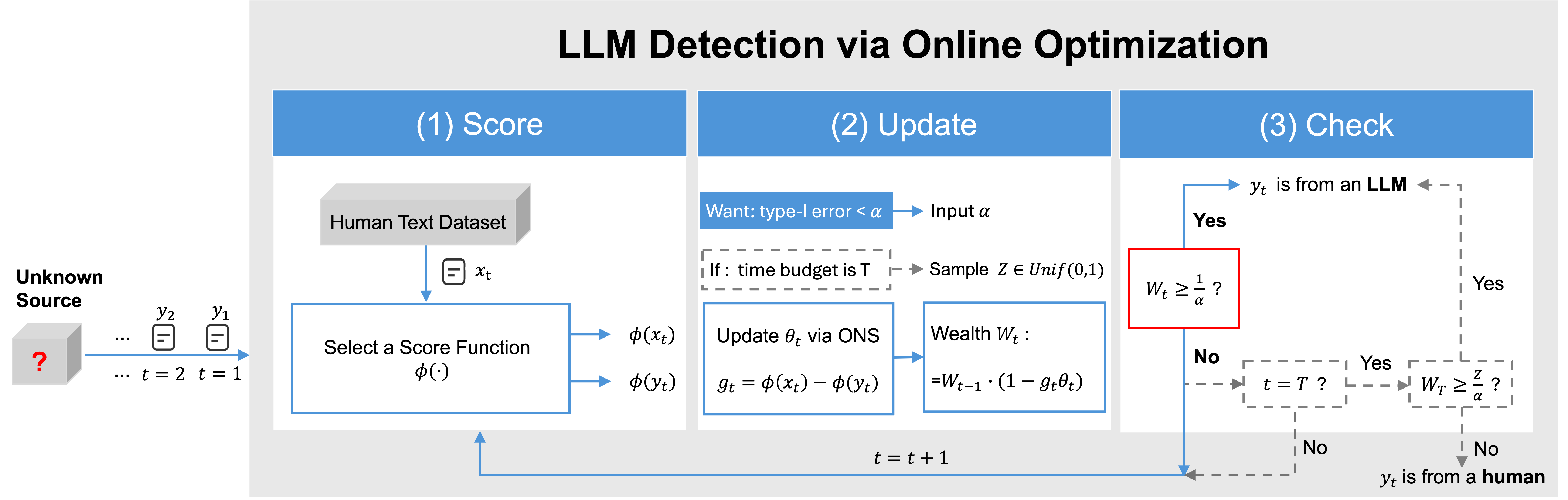
We note that when is true, this is not equivalent to saying that the texts are human-written, as different distributions can share the same mean. However, under the additional assumption of the existence of a good score function which produces scores for machine-generated texts with a mean different from that of human-generated texts , is equivalent to the unknown source being human. Therefore, under this additional assumption, when the unknown source is an LLM, then rejecting the null hypothesis is equivalent to correctly identifying that the source is indeed an LLM. In our experiments, we found that this assumption generally holds empirically for the score functions that we adopt. That is, the empirical mean of significantly differs from that of when each is generated by an LLM. Figure 1 illustrates the process of online detecting LLMs.
Sequential Hypothesis Testing by Online Optimization and Betting. Consider the scenario that an online learner engages in multiple rounds of a game with an initial wealth . In each round of the game, the learner plays a point . Then, the learner receives a fortune after committing , which is , where is the learner’s wealth from the previous round , and can be thought of as “the coin outcome” at that the learner is trying to “bet” on (Orabona and Pál, 2016). Consequently, the dynamic of the wealth of the learner evolves as:
| (2) |
To connect the learner’s game with sequential hypothesis testing, one of the key techniques that will be used in the algorithm design and analysis is Ville’s inequality(Ville, 1939), which states that if is a nonnegative supermartingale, then one has . The idea is that if we can guarantee that the learner’s wealth can remain nonnegative from , then Ville’s inequality can be used to control the type-I error at level simultaneously at all time steps . To see this, let . Then, when (i.e., the null hypothesis holds), the wealth is a P-supermartingale, because
Hence, if the learner’s wealth can remain nonnegative given the initial wealth , we can apply Ville’s inequality to get a provable level- test, since is a nonnegative supermartingale in this case. Another key technique is randomized Ville’s inequality (Ramdas and Manole, 2023) for a nonnegative supermartingale , which states that , where is any -stopping time and is randomly drawn from the uniform distribution in . This inequality becomes particularly handy when there is a time budget in sequential hypothesis testing while maintaining a valid level- test.
We now switch to discussing the control of the type-II error, which occurs when the wealth is not accumulated enough to reject when is true. Therefore, we need a mechanism to enable the online learner in the game quickly increase the wealth under . Related works of sequential hypothesis testing by betting (Shekhar and Ramdas, 2023; Chugg et al., 2023) propose using a no-regret learning algorithm to achieve this. Specifically, a no-regret learner aims to obtain a sublinear regret, which is defined as , where is a benchmark. In our case, we will consider the loss function at to be . The high-level idea is based on the observation that the first term in the regret definition is the log of the learner’s wealth, modulo a minus sign, i.e., , while the second term is that of a benchmark. Therefore, if the learner’s regret can be upper-bounded, say , then the learner’s wealth is lower-bounded as . An online learning algorithm with a small regret bound can help increase the wealth quickly under . We refer the reader to Appendix D for a rigorous argument, where we note that applying a no-regret algorithm to guarantee the learner’s wealth is a neat technique that is well-known in online learning, see e.g., Chapter 9 of Orabona (2019) for more details. Following existing works (Shekhar and Ramdas, 2023; Chugg et al., 2023), we will adopt Online Newton Steps (ONS) (Hazan et al., 2007) in our algorithm.
3 Our Algorithm
We have covered most of the underlying algorithmic design principles of our online method for detecting LLMs, and we are now ready to introduce our algorithm, which is shown in Algorithm 1. Compared to existing works on sequential hypothesis testing via betting (e.g., Shekhar and Ramdas (2023); Chugg et al. (2023)), which assume knowledge of a bound on the magnitude of the “coin outcome" in the learner’s wealth dynamic (2) for all time steps before the testing begins (i.e., assuming prior knowledge of ), we relax this assumption.
Specifically, we consider the scenario where an upper bound on , which is denoted by , is available before updating at each round . Our algorithm then plays a point in the decision space that guarantees the learner’s wealth remains a non-negative supermartingale (Step 11 in Algorithm 1). We note that if the bound of the output of the underlying score function is known a priori, this scenario holds naturally. Otherwise, we can estimate an upper bound for for all based on the first few time steps and execute the algorithm thereafter. One approach is to set the estimate as a conservatively large constant, e.g., twice the maximum value observed in the first few time steps. We observe that this estimate works for our algorithm with most of the score functions that we consider in the experiments. On the other hand, we note that a tighter bound will lead to a faster time to reject when the unknown source is an LLM, as indicated by the following propositions.
Proposition 1.
Algorithm 1 is a level- sequential test with asymptotic power one. Furthermore, if is generated by an LLM, the expected time to declare the unknown source as an LLM is bounded by
| (3) |
where , with , and satisfies with denoting the upper bound of the gradient .
Remark 1. Under the additional assumption of the existence of a good score function that can generate scores with different means for human-written texts and LLM-generated ones, Proposition 1 implies that when the unknown source is declared by Algorithm 1 as an LLM, the probability of this declaration being false will be bounded by . Additionally, if the unknown source is indeed an LLM, then our algorithm can guarantees that it will eventually detect the LLM, since it has asymptotic power one. Moreover, Proposition 1 also provides a non-asymptotic result (see (3)) for bounding the expected time to reject the null hypothesis , which is also the expected time to declare that the unknown source is an LLM. The bound indicates that a larger difference of the means can lead to a shorter time to reject the null .
(Composite Hypotheses.) As Chugg et al. (2023), we also consider the composite hypothesis, which can be formulated as versus . The hypothesis can be equivalently expressed in terms of two hypotheses,
| (4) |
Consequently, the dynamic of the wealth evolves as and respectively, where . We note that both and are within the interval . The composite hypothesis is motivated by the fact that, in practice, even if both sequences of texts and are human-written, they may have been written by different individuals. Therefore, it might be more reasonable to allow for a small difference in their means when defining the null hypothesis .
Proposition 2.
Algorithm 3 in the appendix is a level- sequential test with asymptotic power one, where the wealth for and for are calculated through level- tests. Furthermore, if is generated by an LLM, the expected time to declare the unknown source as an LLM is bounded by
| (5) |
Remark 2. Proposition 2 indicates that even if there is a difference in mean scores between texts written by different humans, the probability that the source is incorrectly declared by Algorithm 3 as an LLM can be controlled below . Besides, our algorithm will eventually declare the source as an LLM if the texts are indeed LLM-generated, as it achieves asymptotic power of one. The expected time to reject and then declare the unknown source as an LLM is bounded (see (5)). The bound implies that smaller and larger will result in a shorter time to reject .
4 Experiments
4.1 Settings
Score Functions. We use score functions in total from the related works for the experiments. As mentioned earlier, a score function takes a text as an input and outputs a score. For example, one of the configurations of our algorithm that we try uses a score function called Likelihood, which is based on the average of the logarithmic probabilities of each token conditioned on its preceding tokens(Solaiman et al., 2019; Hashimoto et al., 2019). More precisely, for a text which consists of tokens, this score function can be formulated as , where denotes the -th token of the text , means the first tokens, and represents the probability computed by a language model used for scoring. The score functions considered in the experiments are: 1. DetectGPT: perturbation discrepancy(Mitchell et al., 2023). 2. Fast-DetectGPT: conditional probability curvature(Bao et al., 2023). 3.LRR: likelihood log-rank ratio(Su et al., 2023). 4. NPR: normalized perturbed log-rank(Su et al., 2023). 5. DNA-GPT: WScore(Yang et al., 2023). 6. Likelihood: mean log probabilities (Solaiman et al., 2019; Hashimoto et al., 2019; Gehrmann et al., 2019). 7. LogRank: averaged log-rank in descending order by probabilities(Gehrmann et al., 2019). 8. Entropy: mean token entropy of the predictive distribution(Gehrmann et al., 2019; Solaiman et al., 2019; Ippolito et al., 2019). 9. RoBERTa-base: a pre-trained classifier(Liu et al., 2019). 10. RoBERTa-large: a larger pre-trained classifier with more layers and parameters(Liu et al., 2019). The first eight score functions calculate scores based on certain statistical properties of texts, with each text’s score computed via a language model. The last two score functions compute scores by using some pre-trained classifiers. For the reader’s convenience, more details about the implementation of the score functions are provided in Appendix B.
LLMs and Datasets. Our experiments focus on the black-box setting(Bao et al., 2023), which means that if is generated by a model , i.e., , a different model will then be used to evaluate the metrics such as the log-probability when calculating . The models and are respectively called the “source model" and “scoring model" for clarity. The black-box setting is a relevant scenario in practice because the source model used for generating the texts to be inferred is likely unknown in practice, which makes it elusive to use the same model to compute the scores.
We construct a dataset that contains some real news and fake ones generated by LLMs for 2024 Olympics. Specifically, we collect 500 news about Paris 2024 Olympic Games from its official website(Olympics, 2024) and then use three source models, Gemini-1.5-Flash, Gemini-1.5-Pro(Google Cloud, 2024a), and PaLM 2(Google Cloud, 2024b; Chowdhery et al., 2023) to generate an equal number of fake news based on the first 30 tokens of each real one respectively. Two scoring models for computing the text scores are considered, which are GPT-Neo-2.7B (Neo-2.7)(Black et al., 2021) and Gemma-2B(Google, 2024). The perturbation model that is required for the score function DetectGPT and NPR is T5-3B(Raffel et al., 2020). For Fast-DetectGPT, the sampling model is GPT-J-6B(Wang and Komatsuzaki, 2021) when scored with Neo-2.7, and Gemma-2B when the scoring model is Gemma-2B. We sample human-written text from a pool of 500 news articles from the XSum dataset(Narayan et al., 2018). We also consider existing datasets from Bao et al. (2023) for the experiments. Details can be found in Appendix H.
Baselines. Our method are compared with two baselines, which adapt the fixed-time permutation test (Good, 2013) to the scenario of the sequential hypothesis testing. Specifically, the first baseline conducts a permutation test after collecting every samples. If the result does not reject , then it will wait and collect another samples to conduct another permutation test on this new batch of samples. This process is repeated until is rejected or the time runs out (i.e., when ). The significance leave parameter of the permutation test is set to be the same constant for each batch, which does not maintain a valid level- test overall. The second baseline is similar to the first one except that the significance level parameter for the -th batch is set to be , with starting from , which aims to ensure that the cumulative type-I error is bounded by via the union bound. The detailed process of the baselines is described in Appendix G.
Parameters of Our Algorithm. All the experiments in the following consider the setting of the composite hypothesis. For the step size , we simply follow the related works (Cutkosky and Orabona, 2018; Chugg et al., 2023; Shekhar and Ramdas, 2023) and let . We consider two scenarios of sequential hypothesis testing in the experiments. The first scenario (oracle) assumes that one has prior knowledge of and , and the performance of our algorithm in this case could be considered as an ideal outcome that it can achieve. For simulating this ideal scenario in the experiments, we let be the absolute difference between the mean scores of XSum texts and 2024 Olympic news, which are datasets of human-written texts. The second scenario considers that we do not have such knowledge a priori, and hence we have to estimate (or ) and specify the value of using the samples collected in the first few times steps, and then the hypothesis testing is started thereafter. In our experiments, we use the first samples from each sequence of and and set to be a constant, which is twice the value of . For estimating , we obtain scores for texts sampled from the XSum dataset and randomly divided them into two groups, and set to twice the average absolute difference between the empirical means of these two groups across random shuffles.
4.2 Experimental Results
The experiments evaluate the performance of our method and baselines under both and . As there is inherent randomness from the observed samples of the texts in the online setting, we repeat runs and report the average results over these runs. Specifically, we report the false positive rate (FPR) under , which is the number of times the source of is incorrectly declared as an LLM when it is actually human, divided by the total of runs. We also report the average time to reject the null under (denoted as Rejection Time ), which is the time our algorithm takes to reject and correctly identify the source when is indeed generated by an LLM. More precisely, the rejection time is the average time at which either or exceeds before ; otherwise, is set to , regardless of whether it rejects at , since the the time budget runs out. The parameter value in Scenario 1 (oracle) is shown in Table 2, and the value for can be found in Table 1 in the appendix. For the estimated and of each sequential testing in Scenario 2, they are displayed in Table 5 and Table 6 respectively in the appendix. Our method and the baselines require specifying the significance level parameter . In our experiments, we try evenly spaced values of the significance level parameter that ranges from to and report the performance of each one.
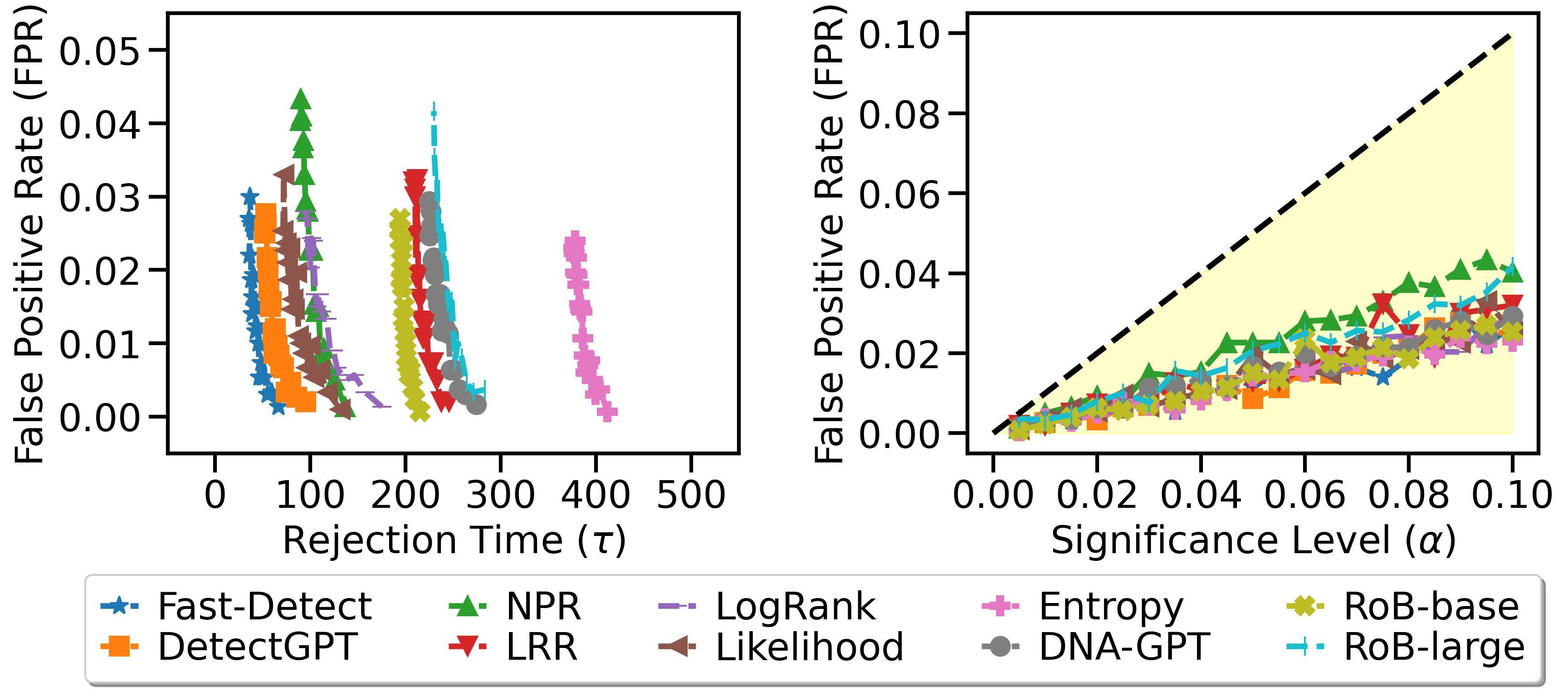
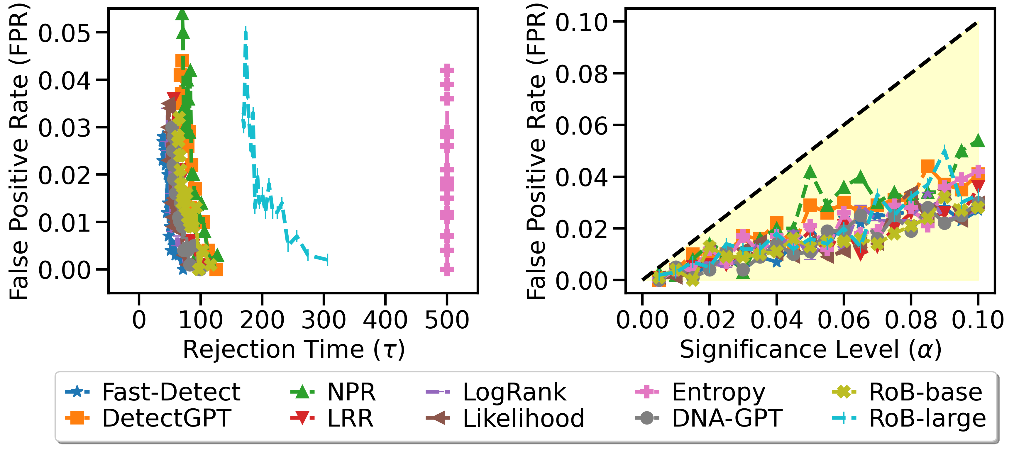
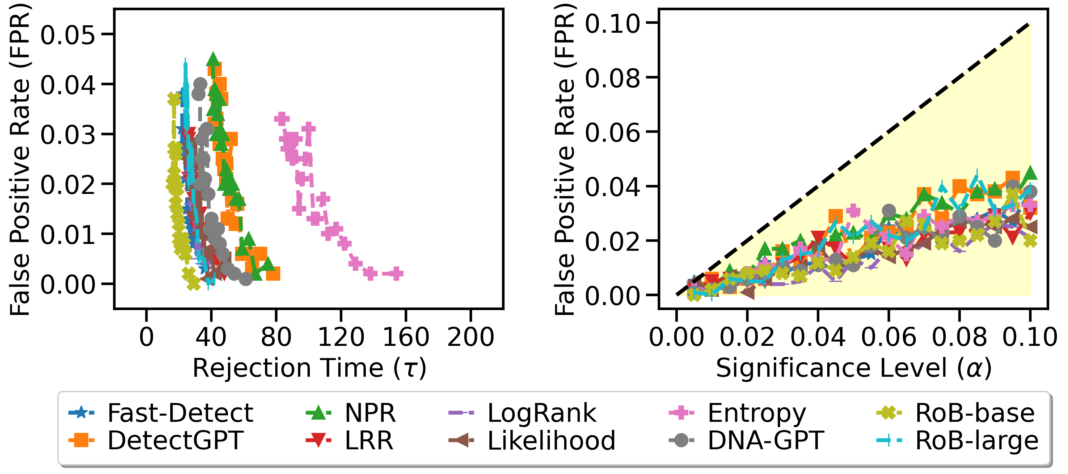
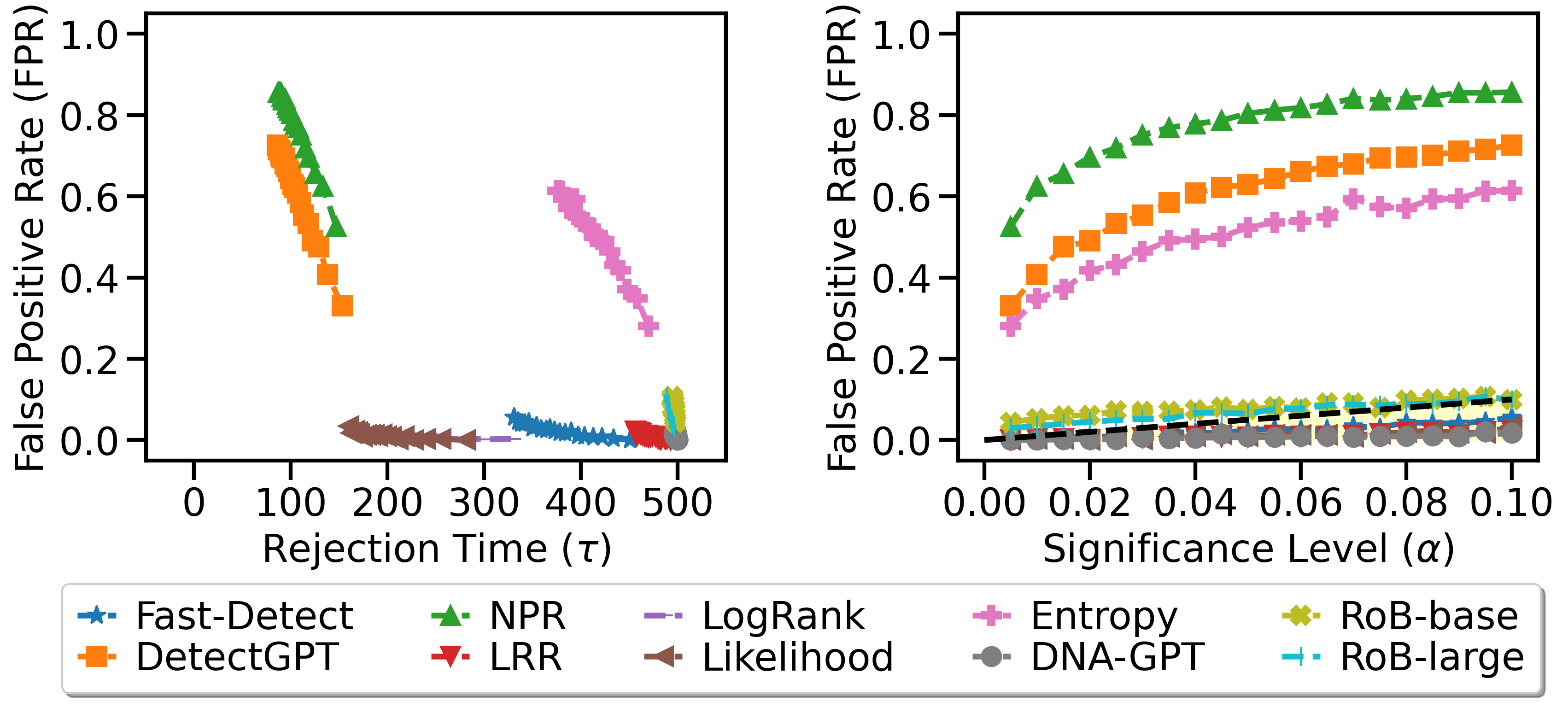
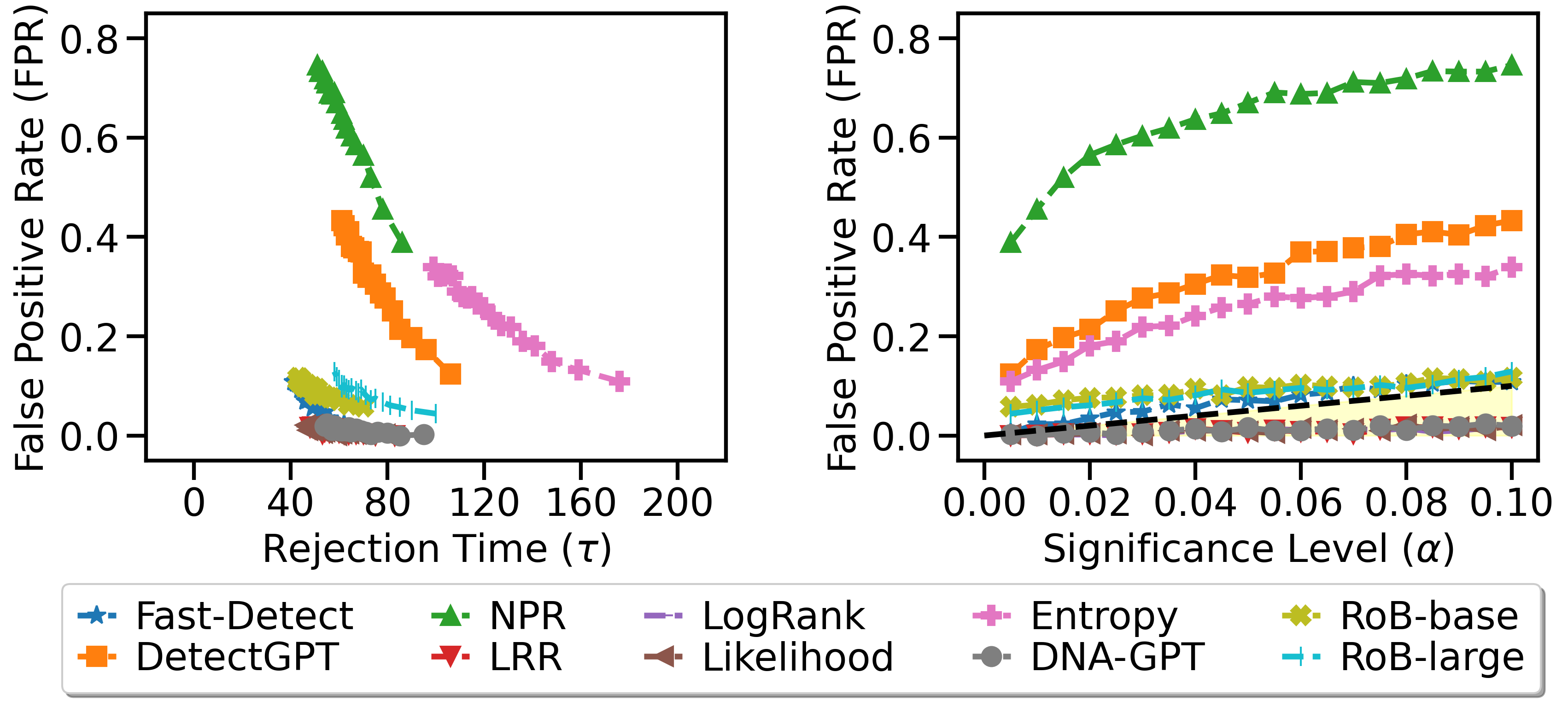
Figure 2 shows the performance of our algorithm with different score functions under Scenario 1 (oracle). Our algorithm consistently controls FPRs below the significance levels and correctly declare the unknown source as an LLM before for all score functions. This includes using the Neo-2.7 or Gemma-2B scoring models to implement eight of these score functions that require a language model. On the plots, each marker represents the average results over runs of our algorithm with a specific score function under different values of the parameter . The subfigures on the left in Figure 2(a) and 2(b) show False Positive Rate (under ) versus Rejection Time (under ); therefore, a curve that is closer to the bottom-left corner is more preferred. From the plot, we can see that the configurations of our algorithm with the score function being Fast-DetectGPT, DetectGPT, or Likelihood have the most competitive performance. When the unknown source is an LLM, they can detect it at time around on average, and the observation is consistent under different language models used for the scoring. The subfigures on the right in Figure 2 show that the FPR is consistently bounded by the chosen value of the significance level parameter .
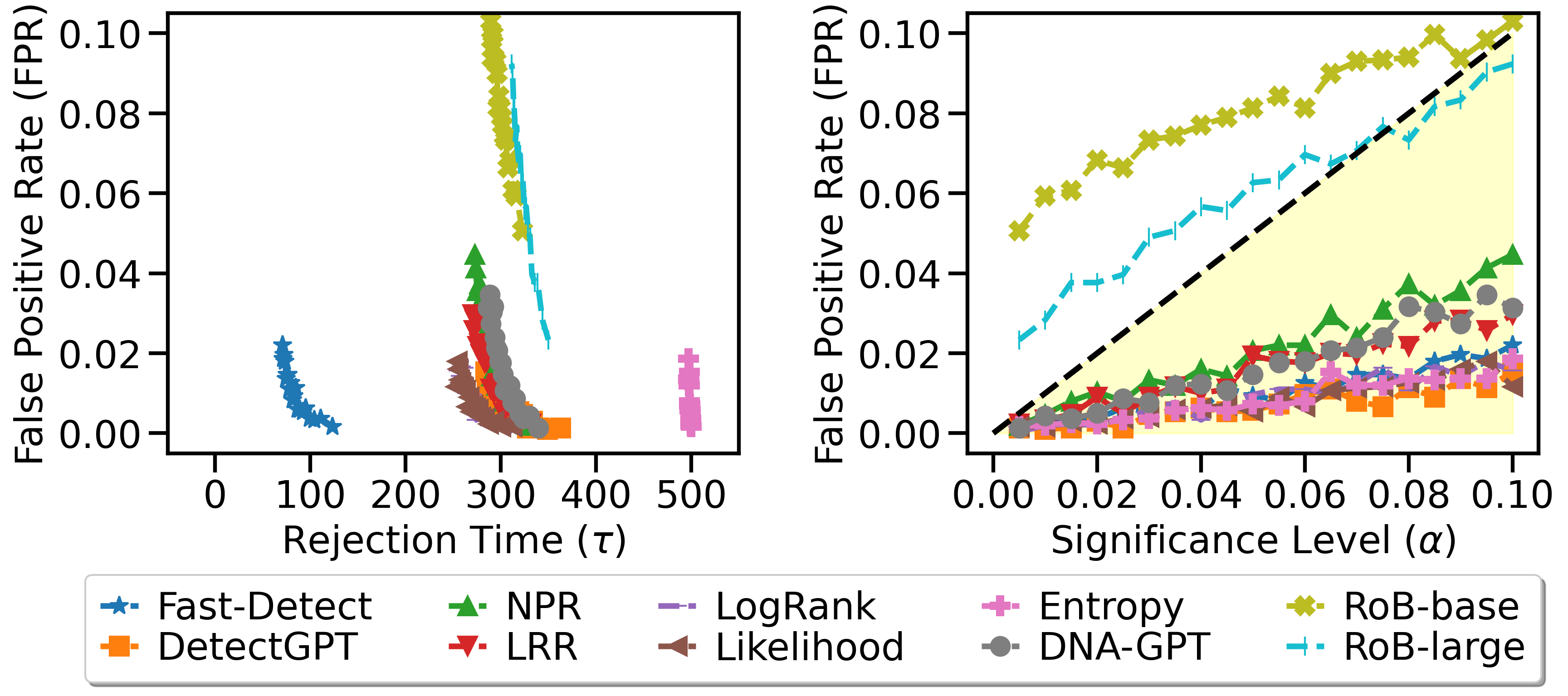
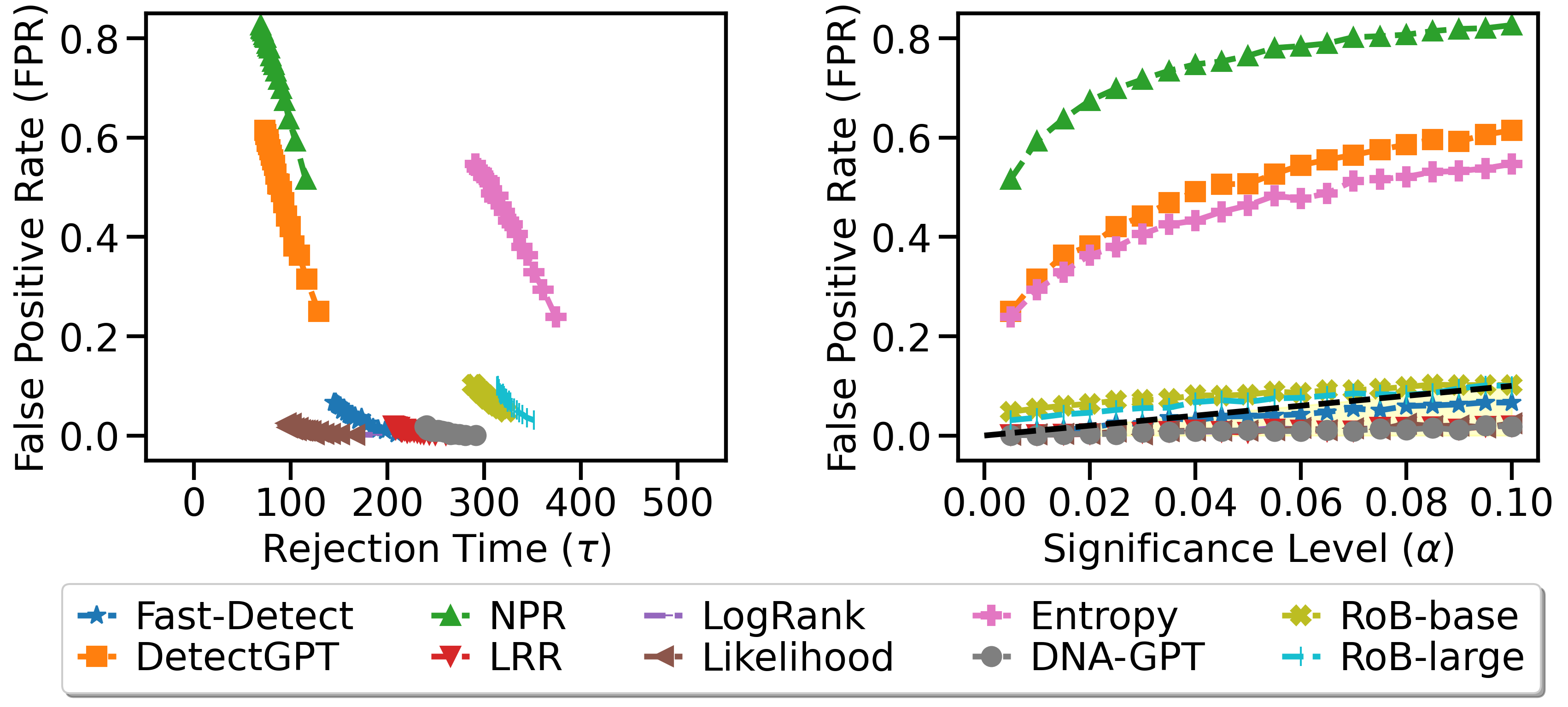
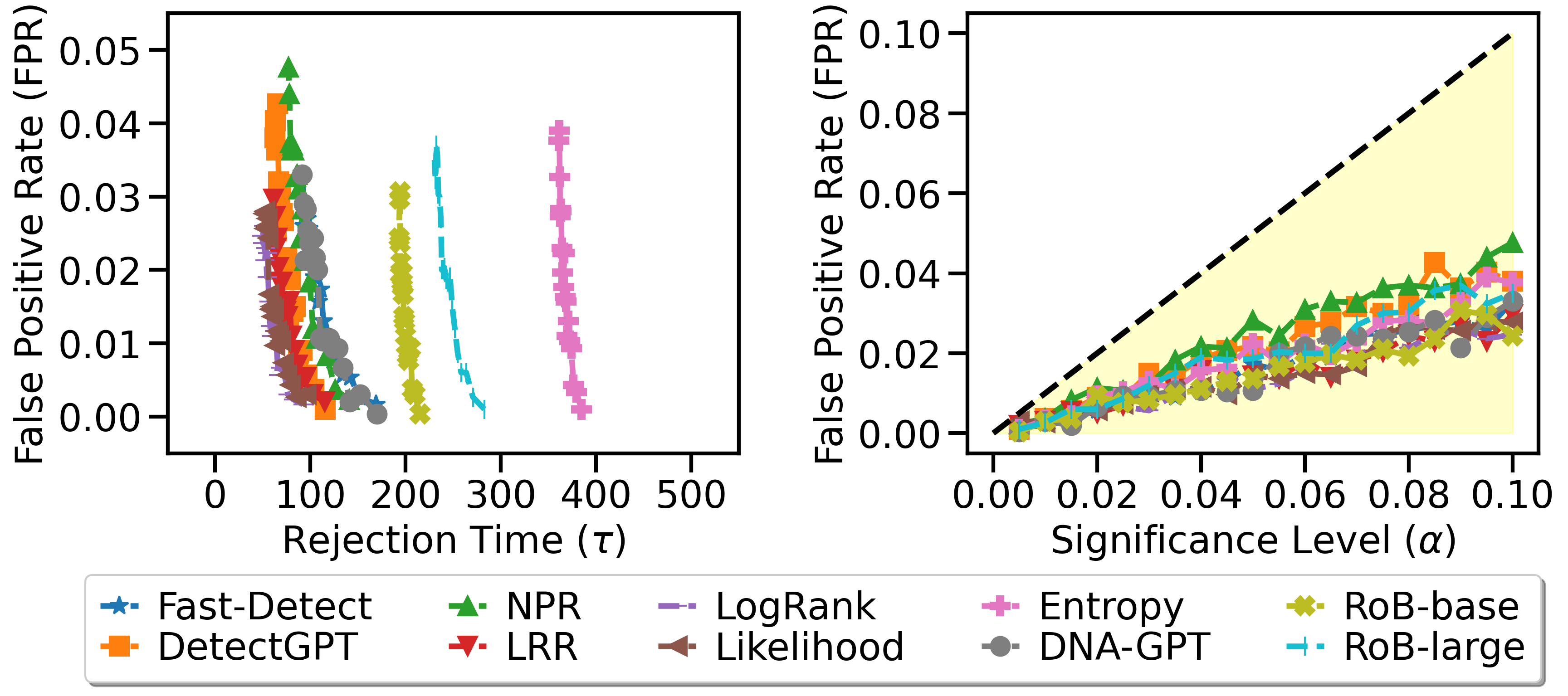
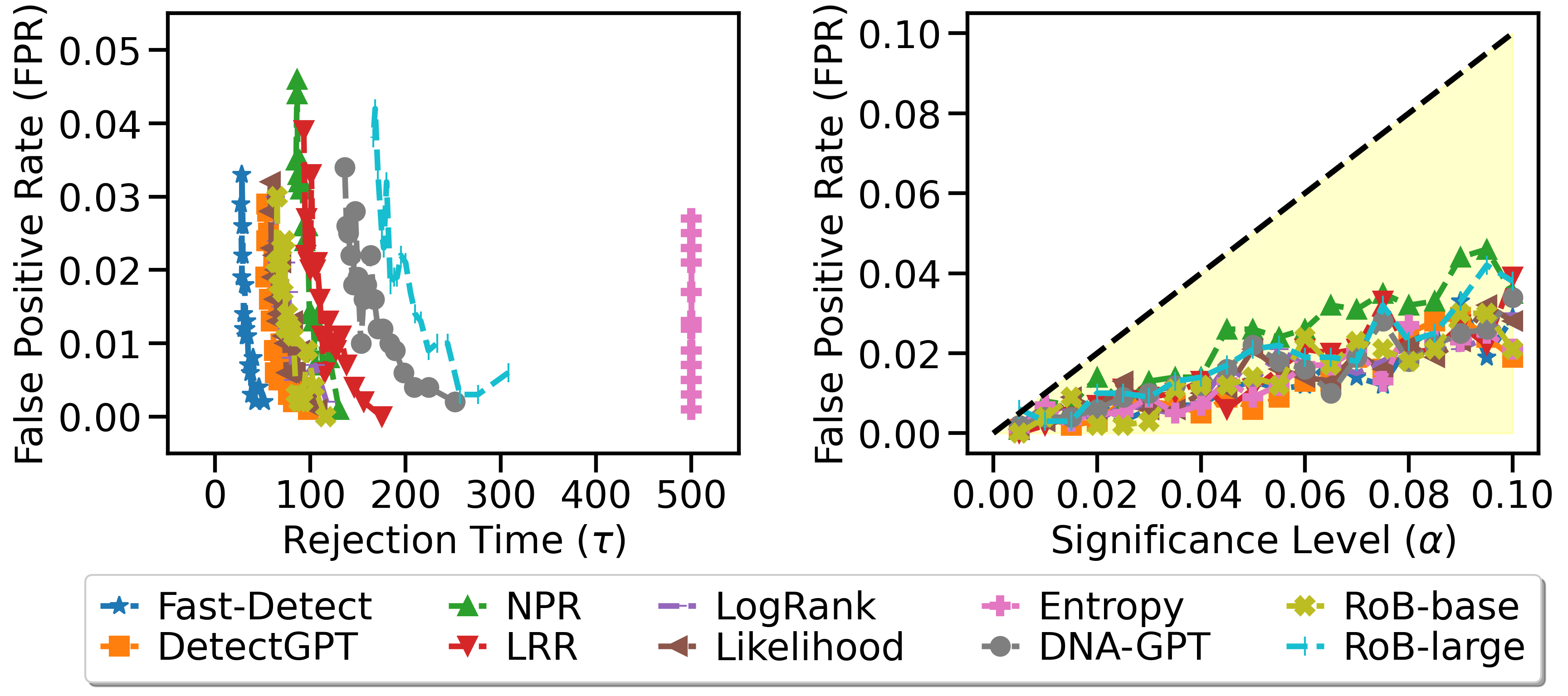
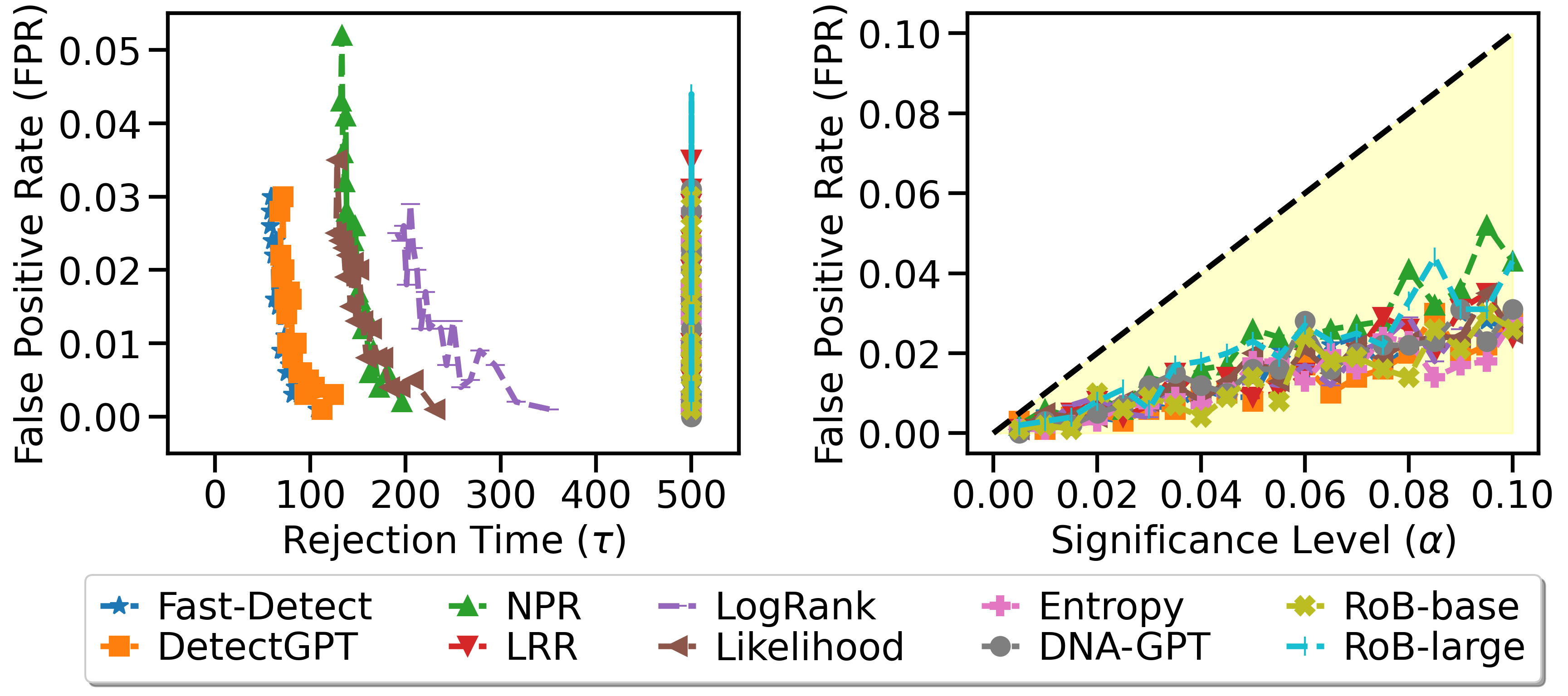
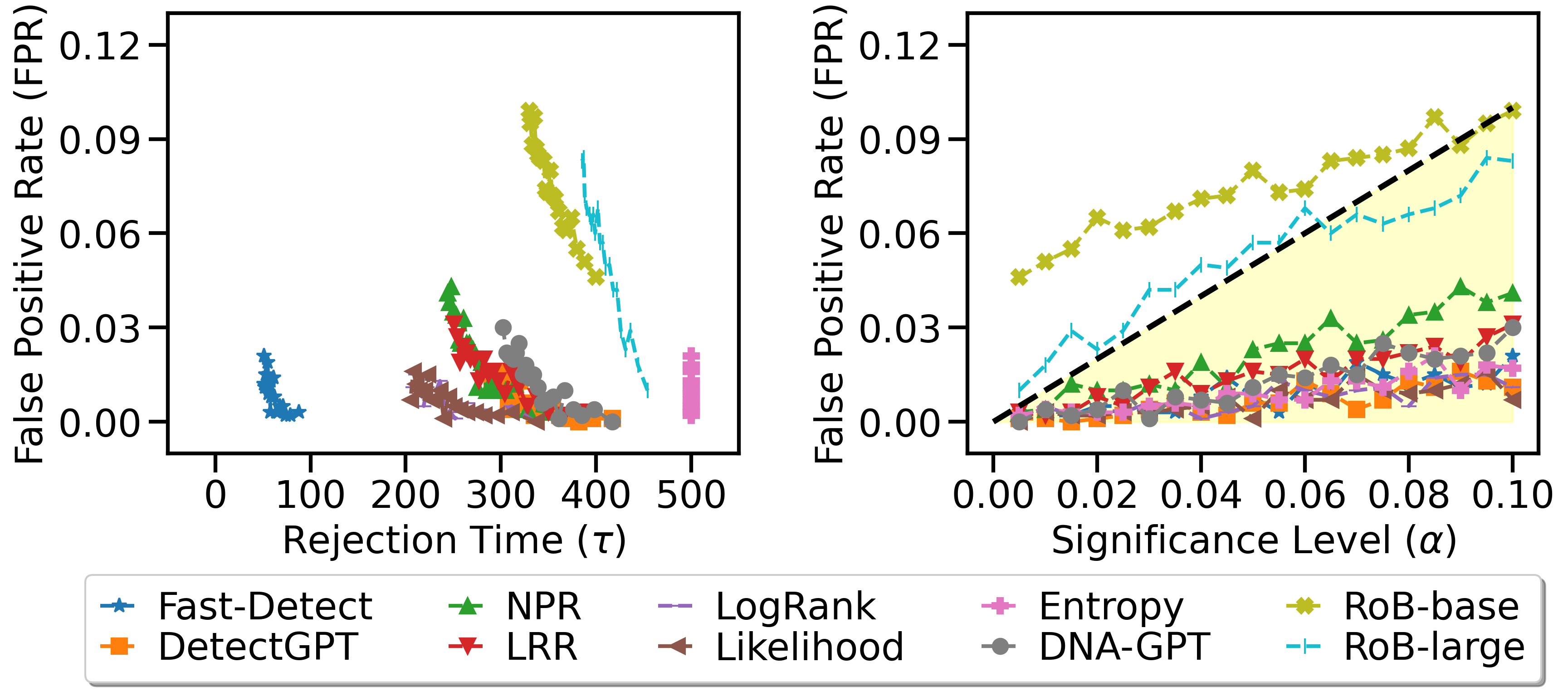
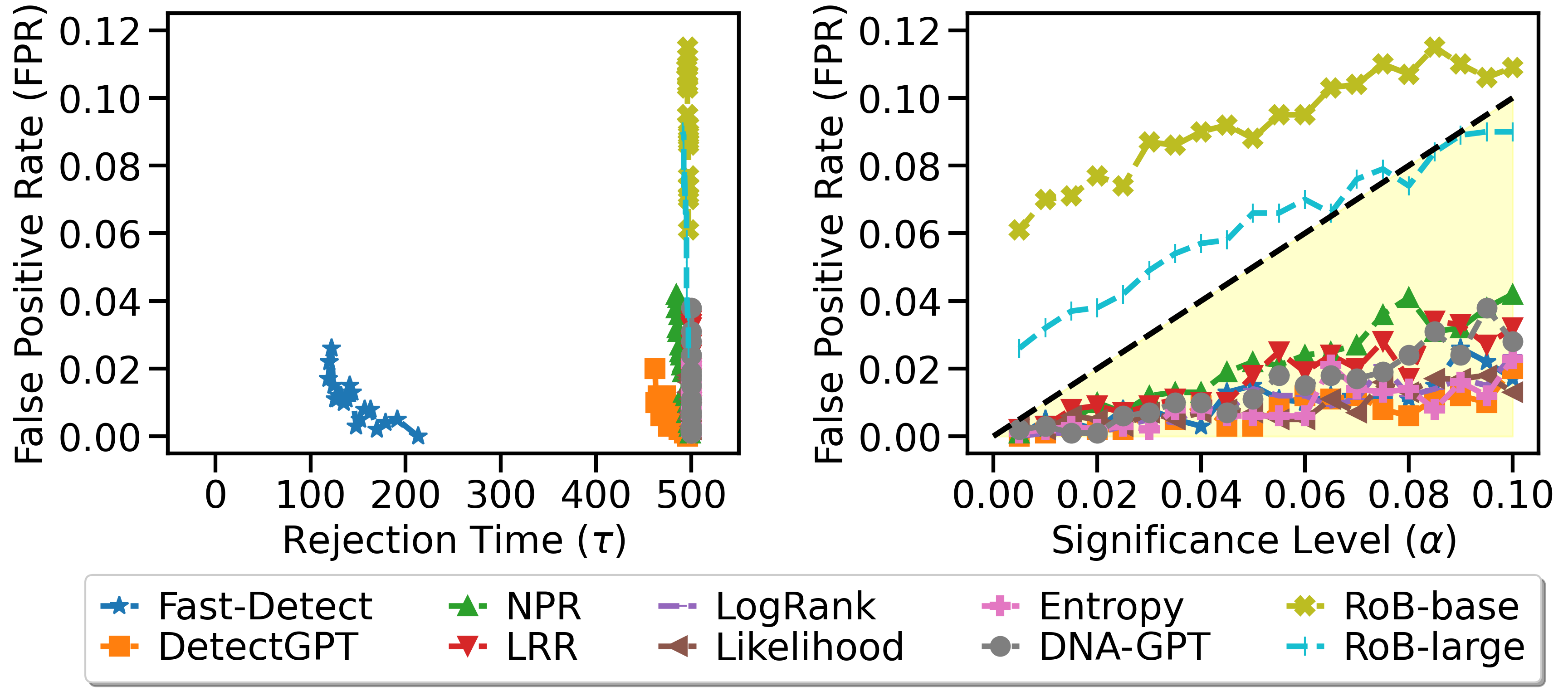
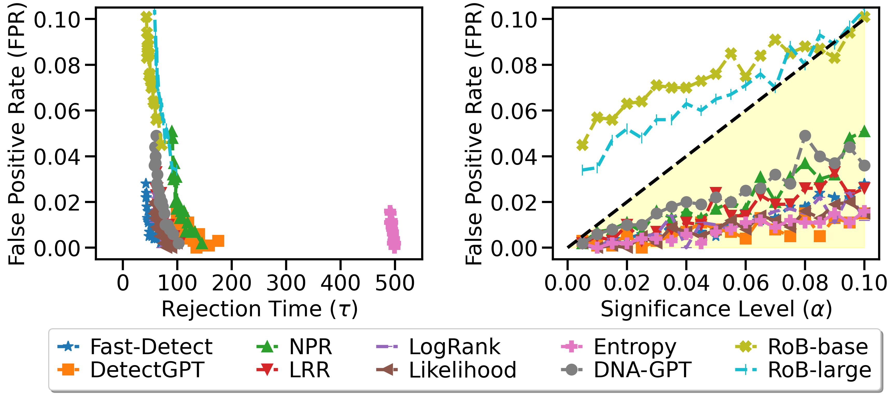
Figure 3 shows the empirical results of our algorithm under Scenario 2, where it has to use the first few samples to specify and before starting the algorithm. Under this scenario, our algorithm equipped with most of the score functions still perform effectively. We observe that our algorithm with 1) Fast-DetectGPT as the score function and Neo-2.7 as the language model for computing the score, and with 2) Likelihood as the score function and Gemma-2B for computing the value of have the best performance under this scenario. Compared to the first case where the oracle of and is available and exploited, these two configurations only result in a slight degradation of the performance under Scenario 2, and we note that our algorithm can only start updating after the first time steps under this scenario. We observe that the bound of that we estimated using the samples collected from first time steps is significantly larger than the tightest bound of in most of the runs where we refer the reader to Table 2, 6 in the appendix for details, which explains why most of the configurations under Scenario 2 need a longer time to detect LLMs, as predicted by our propositions. We also observe that the configurations with two supervised classifiers (RoBERTa-based and RoBERTa-large) and the combinations of a couple of score functions and the scoring model Gemma-2B do not strictly control FPRs across all significance levels. This is because the estimated for these score functions is not large enough to ensure that the wealth remains nonnegative at all time points . That is, we observed for some in the experiments, and hence the wealth is no longer a non-negative supermartingale, which prevents the application of Ville’s inequality to guarantee a level- test. Nevertheless, our algorithm with eight score functions that utilize the scoring model Neo-2.7 can still effectively control type-I error and detect LLMs by around .
In Appendix H, we provide more experimental results, including those using existing datasets from Bao et al. (2023) for simulating the sequential testing, where our algorithm on these datasets also performs effectively. Moreover, we found that the rejection time is influenced by the relative magnitude of and , as predicted by our propositions, and the details are provided in Appendix G. From the experimental results, when the knowledge of and is not available beforehand, as long as the estimated and guarantee a nonnegative supermartingale, and the estimated is greater than or equal to the actual absolute difference in the empirical mean scores of two sequences of human texts, our algorithm can maintain a sequential valid level- test and efficiently detect LLMs.
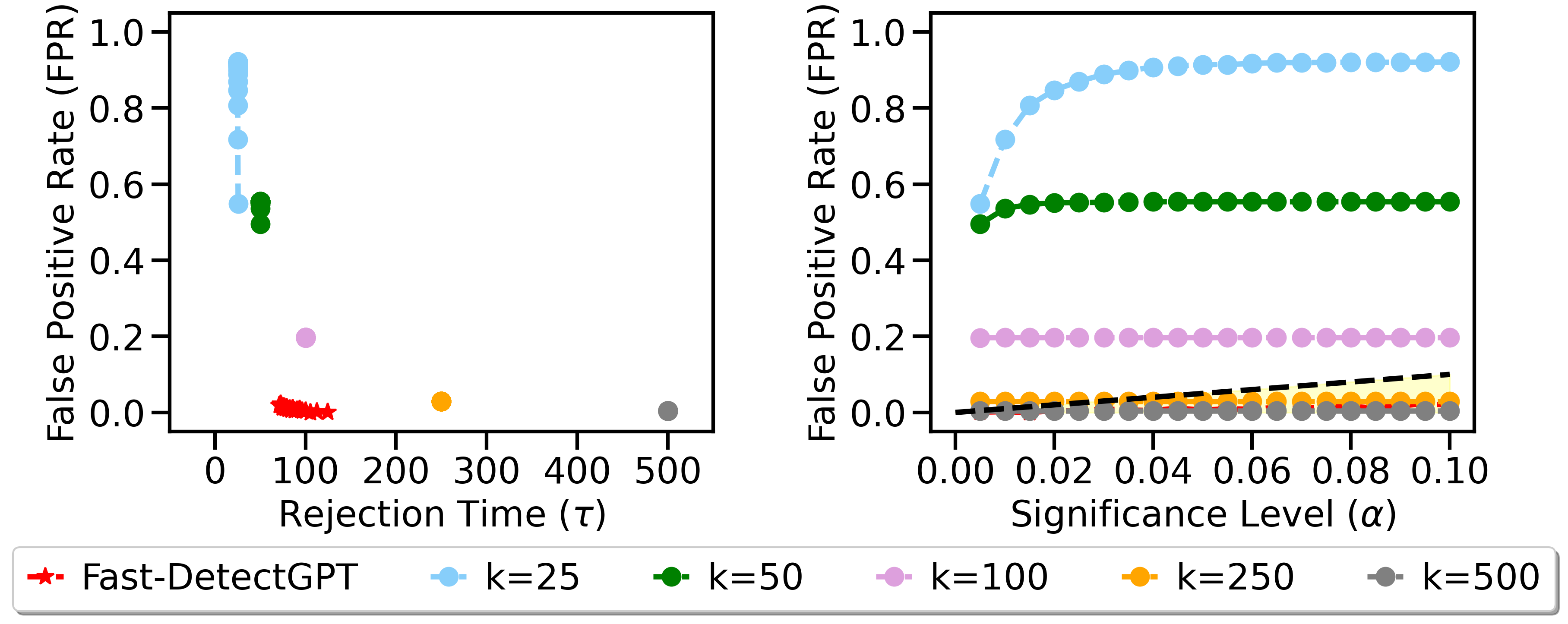
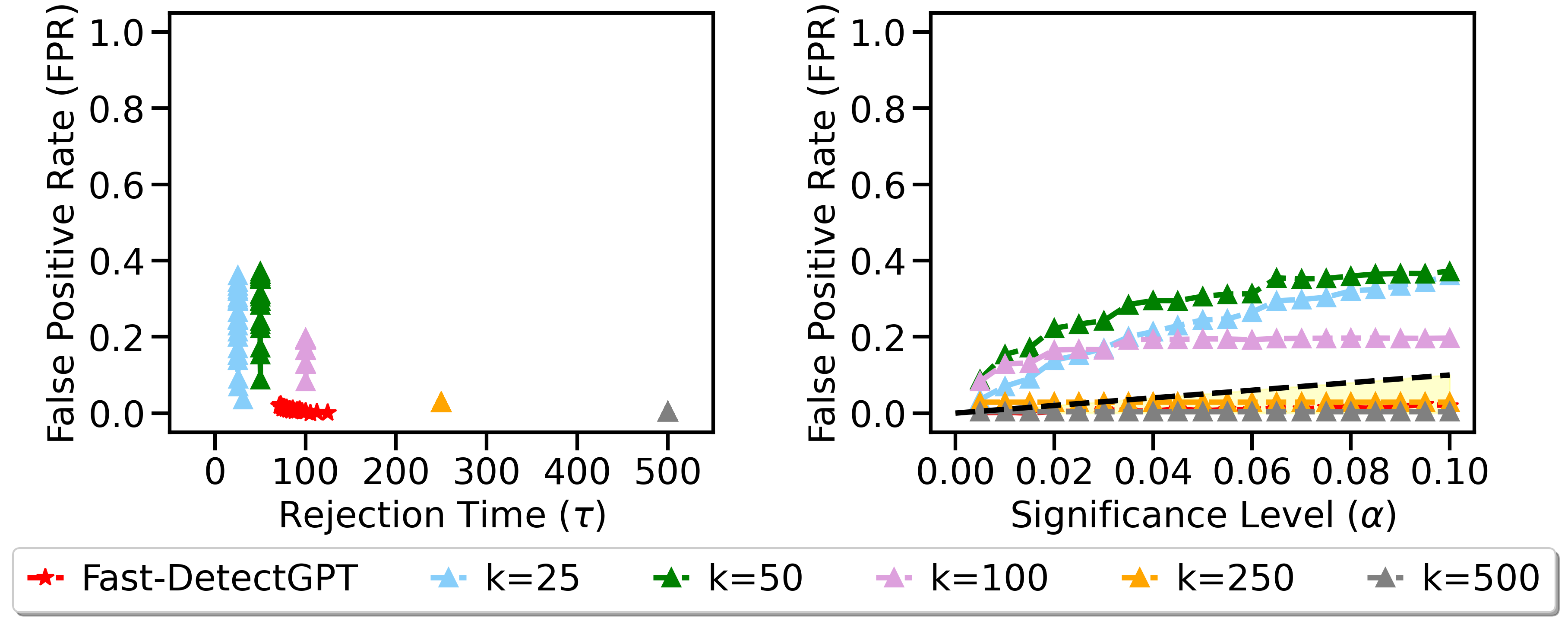
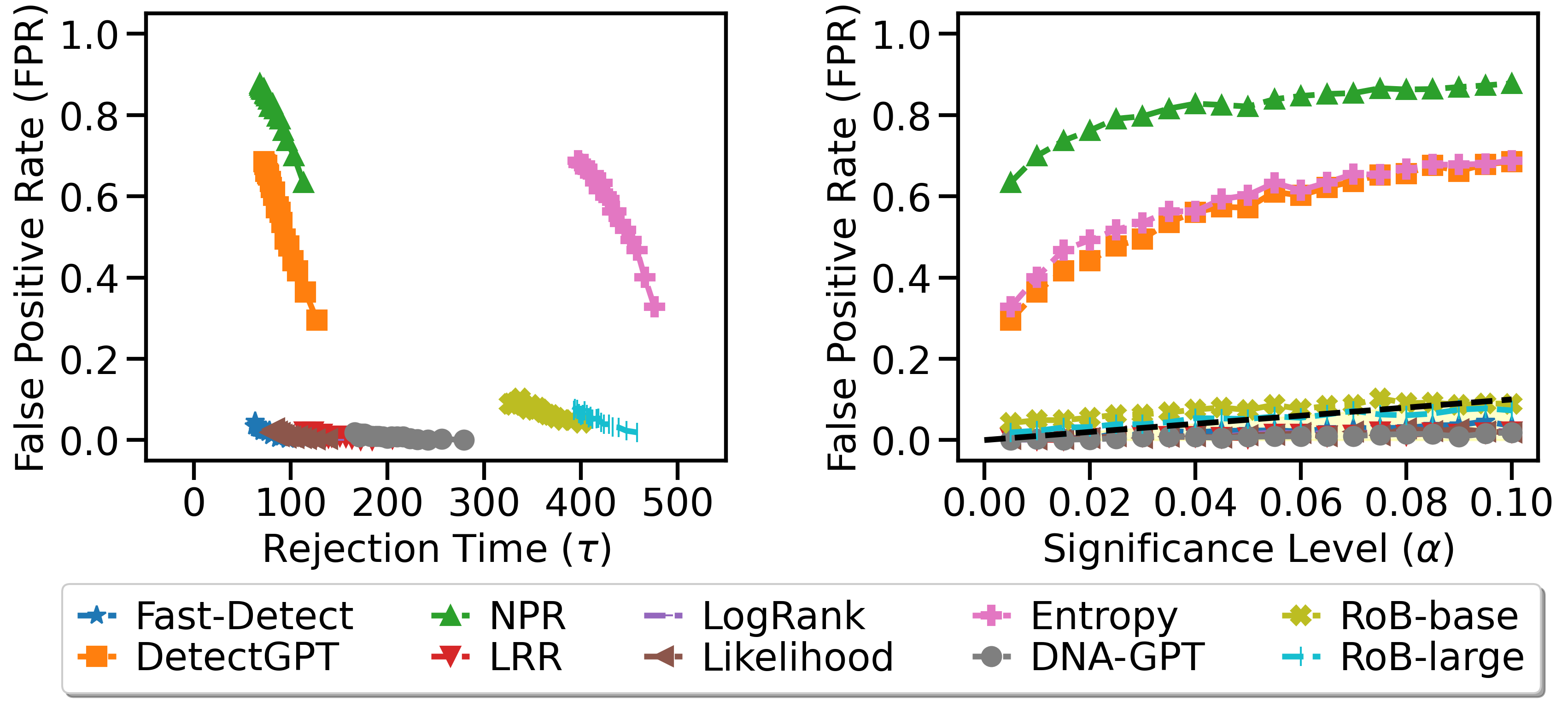
Comparisons with Baselines. In this part, we use the score function of Fast-DetectGPT and scoring model Neo-2.7 to get text scores, and then compare the performance of our method with two baselines that adapt the fixed-time permutation test to the sequential hypothesis setting. Batch sizes are considered for the baselines. We set the estimated and values the same as in Scenario 2. The baselines are also implemented in a manner to conduct the composite hypothesis test. We observe a significant difference between the scores of XSum texts and machine-generated news, which causes the baselines of the permutation test to reject the null hypothesis most of the time immediately after receiving the first batch. This in turn results in the nearly vertical lines observed in the left subfigure of Figure 4(a) and Figure 4(b), where the averaged rejection time across 1000 repeated tests closely approximates the batch size for each of the 20 significance levels . On the other hand, we observe that when is true, the baselines might not be a valid -test, even with a corrected significance level. This arises from the increased variability of text scores introduced by smaller batch sizes, which results in observed absolute differences in means that may exceed the value under .
Our method can quickly detect an LLM while keeping the false positive rates (FPRs) below the specified significance levels, which is a delicate balance that can be difficult for the baselines to achieve. Without prior knowledge of the value, the baselines of permutation tests may fail to control the type-I error with small batch sizes and cannot quickly reject the null hypothesis while ensuring that FPRs remain below , unlike our method.
5 Limitations and Outlooks
In this paper, we demonstrate that our algorithm, which builds on the score functions of offline detectors, can rapidly determine whether a stream of text is generated by an LLM and provides strong statistical guarantees. Specifically, it controls the type-I error rate below the significance level, ensures that the source of LLM-generated texts can eventually be identified, and guarantees an upper bound on the expected time to correctly declare the unknown source as an LLM under a mild assumption. Although the choice of detector can influence the algorithm’s performance and some parameters related to text scores need to be predefined before receiving the text, our experimental results show that most existing detectors provide effective score functions, and our method performs well in most cases when using estimated values of parameters based on text scores from the first few time steps. To further enhance its efficacy, it may be worthwhile to design score functions tailored to the sequential setting, improve parameter estimations with scores from more time steps, and study the trade-offs between delaying the start of testing and obtaining more reliable estimates.
Moreover, our algorithm could potentially be used as an effective tool to promptly identify and mitigate the misuse of LLMs in generating texts, such as identifying users who post LLM-generated comments in forums to manipulate public opinion, monitoring social media accounts that disseminate harmful information generated by LLMs, and rapidly detecting sources of fake news generated by LLMs on public websites. Exploring these applications could be a promising direction.
References
- Yuan et al. [2022] Ann Yuan, Andy Coenen, Emily Reif, and Daphne Ippolito. Wordcraft: story writing with large language models. In Proceedings of the 27th International Conference on Intelligent User Interfaces, pages 841–852, 2022.
- Kasneci et al. [2023] Enkelejda Kasneci, Kathrin Seßler, Stefan Küchemann, Maria Bannert, Daryna Dementieva, Frank Fischer, Urs Gasser, Georg Groh, Stephan Günnemann, Eyke Hüllermeier, et al. Chatgpt for good? on opportunities and challenges of large language models for education. Learning and individual differences, 103:102274, 2023.
- Zhang et al. [2024] Tianyi Zhang, Faisal Ladhak, Esin Durmus, Percy Liang, Kathleen McKeown, and Tatsunori B Hashimoto. Benchmarking large language models for news summarization. Transactions of the Association for Computational Linguistics, 12:39–57, 2024.
- Zellers et al. [2019] Rowan Zellers, Ari Holtzman, Hannah Rashkin, Yonatan Bisk, Ali Farhadi, Franziska Roesner, and Yejin Choi. Defending against neural fake news. Advances in neural information processing systems, 32, 2019.
- Lin et al. [2021] Stephanie Lin, Jacob Hilton, and Owain Evans. Truthfulqa: Measuring how models mimic human falsehoods. arXiv preprint arXiv:2109.07958, 2021.
- Chen and Shu [2023] Canyu Chen and Kai Shu. Can LLM-generated misinformation be detected? arXiv preprint arXiv:2309.13788, 2023.
- Bommasani et al. [2021] Rishi Bommasani, Drew A Hudson, Ehsan Adeli, Russ Altman, Simran Arora, Sydney von Arx, Michael S Bernstein, Jeannette Bohg, Antoine Bosselut, Emma Brunskill, et al. On the opportunities and risks of foundation models. arXiv preprint arXiv:2108.07258, 2021.
- Lee et al. [2023] Jooyoung Lee, Thai Le, Jinghui Chen, and Dongwon Lee. Do language models plagiarize? In Proceedings of the ACM Web Conference 2023, pages 3637–3647, 2023.
- Adelani et al. [2020] David Ifeoluwa Adelani, Haotian Mai, Fuming Fang, Huy H Nguyen, Junichi Yamagishi, and Isao Echizen. Generating sentiment-preserving fake online reviews using neural language models and their human-and machine-based detection. In Advanced information networking and applications: Proceedings of the 34th international conference on advanced information networking and applications (AINA-2020), pages 1341–1354. Springer, 2020.
- Stokel-Walker [2022] Chris Stokel-Walker. Ai bot chatgpt writes smart essays-should academics worry? Nature, 2022.
- Susnjak and McIntosh [2024] Teo Susnjak and Timothy R McIntosh. Chatgpt: The end of online exam integrity? Education Sciences, 14(6):656, 2024.
- Jawahar et al. [2020] Ganesh Jawahar, Muhammad Abdul-Mageed, and Laks VS Lakshmanan. Automatic detection of machine generated text: A critical survey. arXiv preprint arXiv:2011.01314, 2020.
- Lavergne et al. [2008] Thomas Lavergne, Tanguy Urvoy, and François Yvon. Detecting fake content with relative entropy scoring. Pan, 8(27-31):4, 2008.
- Hashimoto et al. [2019] Tatsunori B Hashimoto, Hugh Zhang, and Percy Liang. Unifying human and statistical evaluation for natural language generation. arXiv preprint arXiv:1904.02792, 2019.
- Gehrmann et al. [2019] Sebastian Gehrmann, Hendrik Strobelt, and Alexander M Rush. Gltr: Statistical detection and visualization of generated text. arXiv preprint arXiv:1906.04043, 2019.
- Mitchell et al. [2023] Eric Mitchell, Yoonho Lee, Alexander Khazatsky, Christopher D Manning, and Chelsea Finn. Detectgpt: Zero-shot machine-generated text detection using probability curvature. In International Conference on Machine Learning, pages 24950–24962. PMLR, 2023.
- Su et al. [2023] Jinyan Su, Terry Yue Zhuo, Di Wang, and Preslav Nakov. Detectllm: Leveraging log rank information for zero-shot detection of machine-generated text. arXiv preprint arXiv:2306.05540, 2023.
- Bao et al. [2023] Guangsheng Bao, Yanbin Zhao, Zhiyang Teng, Linyi Yang, and Yue Zhang. Fast-detectgpt: Efficient zero-shot detection of machine-generated text via conditional probability curvature. arXiv preprint arXiv:2310.05130, 2023.
- Solaiman et al. [2019] Irene Solaiman, Miles Brundage, Jack Clark, Amanda Askell, Ariel Herbert-Voss, Jeff Wu, Alec Radford, Gretchen Krueger, Jong Wook Kim, Sarah Kreps, et al. Release strategies and the social impacts of language models. arXiv preprint arXiv:1908.09203, 2019.
- Bakhtin et al. [2019] Anton Bakhtin, Sam Gross, Myle Ott, Yuntian Deng, Marc’Aurelio Ranzato, and Arthur Szlam. Real or fake? learning to discriminate machine from human generated text. arXiv preprint arXiv:1906.03351, 2019.
- Ippolito et al. [2019] Daphne Ippolito, Daniel Duckworth, Chris Callison-Burch, and Douglas Eck. Automatic detection of generated text is easiest when humans are fooled. arXiv preprint arXiv:1911.00650, 2019.
- Tian [2023] Edward Tian. Gptzero: An ai text detector, 2023. URL https://gptzero.me/. URL https://gptzero.me/.
- Uchendu et al. [2020] Adaku Uchendu, Thai Le, Kai Shu, and Dongwon Lee. Authorship attribution for neural text generation. In Proceedings of the 2020 conference on empirical methods in natural language processing (EMNLP), pages 8384–8395, 2020.
- Fagni et al. [2021] Tiziano Fagni, Fabrizio Falchi, Margherita Gambini, Antonio Martella, and Maurizio Tesconi. Tweepfake: About detecting deepfake tweets. Plos one, 16(5):e0251415, 2021.
- Abdelnabi and Fritz [2021] Sahar Abdelnabi and Mario Fritz. Adversarial watermarking transformer: Towards tracing text provenance with data hiding. In 2021 IEEE Symposium on Security and Privacy (SP), pages 121–140. IEEE, 2021.
- Zhao et al. [2023] Xuandong Zhao, Prabhanjan Ananth, Lei Li, and Yu-Xiang Wang. Provable robust watermarking for ai-generated text. arXiv preprint arXiv:2306.17439, 2023.
- Kirchenbauer et al. [2023] John Kirchenbauer, Jonas Geiping, Yuxin Wen, Jonathan Katz, Ian Miers, and Tom Goldstein. A watermark for large language models. In International Conference on Machine Learning, pages 17061–17084. PMLR, 2023.
- Christ et al. [2024] Miranda Christ, Sam Gunn, and Or Zamir. Undetectable watermarks for language models. In The Thirty Seventh Annual Conference on Learning Theory, pages 1125–1139. PMLR, 2024.
- Selyukh [2017] A Selyukh. Fcc repeals ‘net neutrality’rules for internet providers. NPR (accessed 13 October 2020), 2017.
- Weiss [2019] Max Weiss. Deepfake bot submissions to federal public comment websites cannot be distinguished from human submissions. Technology Science, 2019121801, 2019.
- Kao [2017] J. Kao. More than a million pro-repeal net neutrality comments were likely faked. Hacker Noon, Nov 2017. URL https://hackernoon.com/more-than-a-million-pro-repeal-net-neutrality-comments-were-likely-faked-e9f0e3ed36a6.
- Fröhling and Zubiaga [2021] Leon Fröhling and Arkaitz Zubiaga. Feature-based detection of automated language models: tackling gpt-2, gpt-3 and grover. PeerJ Computer Science, 7:e443, 2021.
- Kilcher [2022] Y. Kilcher. This is the worst ai ever, June 2022. URL https://www.linkedin.com/posts/ykilcher_gpt-4chan-this-is-the-worst-ai-ever-activity-6938520423496081409-Twxg. LinkedIn post.
- Ferrara et al. [2016] Emilio Ferrara, Onur Varol, Clayton Davis, Filippo Menczer, and Alessandro Flammini. The rise of social bots. Communications of the ACM, 59(7):96–104, 2016.
- Belz [2019] Anya Belz. Fully automatic journalism: we need to talk about nonfake news generation. In Conference for truth and trust online, 2019.
- Shafer [2021] Glenn Shafer. Testing by betting: A strategy for statistical and scientific communication. Journal of the Royal Statistical Society Series A: Statistics in Society, 184(2):407–431, 2021.
- Ramdas et al. [2023] Aaditya Ramdas, Peter Grünwald, Vladimir Vovk, and Glenn Shafer. Game-theoretic statistics and safe anytime-valid inference. Statistical Science, 38(4):576–601, 2023.
- Shekhar and Ramdas [2023] Shubhanshu Shekhar and Aaditya Ramdas. Nonparametric two-sample testing by betting. IEEE Transactions on Information Theory, 2023.
- Balsubramani and Ramdas [2015] Akshay Balsubramani and Aaditya Ramdas. Sequential nonparametric testing with the law of the iterated logarithm. arXiv preprint arXiv:1506.03486, 2015.
- Garson [2012] G David Garson. Testing statistical assumptions, 2012.
- Good [2013] Phillip Good. Permutation tests: a practical guide to resampling methods for testing hypotheses. Springer Science & Business Media, 2013.
- Tartakovsky et al. [2014] Alexander Tartakovsky, Igor Nikiforov, and Michele Basseville. Sequential analysis: Hypothesis testing and changepoint detection. CRC press, 2014.
- Yang et al. [2023] Xianjun Yang, Wei Cheng, Yue Wu, Linda Petzold, William Yang Wang, and Haifeng Chen. Dna-gpt: Divergent n-gram analysis for training-free detection of gpt-generated text. arXiv preprint arXiv:2305.17359, 2023.
- Chugg et al. [2023] Ben Chugg, Santiago Cortes-Gomez, Bryan Wilder, and Aaditya Ramdas. Auditing fairness by betting. Advances in Neural Information Processing Systems, 36:6070–6091, 2023.
- Orabona and Pál [2016] Francesco Orabona and Dávid Pál. Coin betting and parameter-free online learning. Advances in Neural Information Processing Systems, 29, 2016.
- Ville [1939] Jean Ville. Etude critique de la notion de collectif. Gauthier-Villars Paris, 1939.
- Ramdas and Manole [2023] Aaditya Ramdas and Tudor Manole. Randomized and exchangeable improvements of markov’s, chebyshev’s and chernoff’s inequalities. arXiv preprint arXiv:2304.02611, 2023.
- Orabona [2019] Francesco Orabona. A modern introduction to online learning. arXiv preprint arXiv:1912.13213, 2019.
- Hazan et al. [2007] Elad Hazan, Amit Agarwal, and Satyen Kale. Logarithmic regret algorithms for online convex optimization. Machine Learning, 69(2):169–192, 2007.
- Liu et al. [2019] Yinhan Liu, Myle Ott, Naman Goyal, Jingfei Du, Mandar Joshi, Danqi Chen, Omer Levy, Mike Lewis, Luke Zettlemoyer, and Veselin Stoyanov. Roberta: A robustly optimized bert pretraining approach. arXiv preprint arXiv:1907.11692, 2019.
- Olympics [2024] Olympics. Olympic games news, 2024. URL https://olympics.com/en/.
- Google Cloud [2024a] Google Cloud. Vertex ai: Machine learning model management, 2024a. URL https://cloud.google.com/vertex-ai?hl=zh_cn.
- Google Cloud [2024b] Google Cloud. Reference for text models in vertex ai, 2024b. URL https://cloud.google.com/vertex-ai/generative-ai/docs/model-reference/text?hl=zh-cn.
- Chowdhery et al. [2023] Aakanksha Chowdhery, Sharan Narang, Jacob Devlin, Maarten Bosma, Gaurav Mishra, Adam Roberts, Paul Barham, Hyung Won Chung, Charles Sutton, Sebastian Gehrmann, et al. Palm: Scaling language modeling with pathways. Journal of Machine Learning Research, 24(240):1–113, 2023.
- Black et al. [2021] Sid Black, Leo Gao, Phil Wang, Connor Leahy, and Stella Biderman. Gpt-neo: Large scale autoregressive language modeling with mesh-tensorflow. 2021. URL https://api.semanticscholar.org/CorpusID:245758737.
- Google [2024] Google. Gemma-2b model on hugging face, 2024. URL https://huggingface.co/google/gemma-2b.
- Raffel et al. [2020] Colin Raffel, Noam Shazeer, Adam Roberts, Katherine Lee, Sharan Narang, Michael Matena, Yanqi Zhou, Wei Li, and Peter J Liu. Exploring the limits of transfer learning with a unified text-to-text transformer. Journal of machine learning research, 21(140):1–67, 2020.
- Wang and Komatsuzaki [2021] Ben Wang and Aran Komatsuzaki. Gpt-j-6b: A 6 billion parameter autoregressive language model, 2021.
- Narayan et al. [2018] Shashi Narayan, Shay B Cohen, and Mirella Lapata. Don’t give me the details, just the summary! topic-aware convolutional neural networks for extreme summarization. arXiv preprint arXiv:1808.08745, 2018.
- Cutkosky and Orabona [2018] Ashok Cutkosky and Francesco Orabona. Black-box reductions for parameter-free online learning in banach spaces. In Conference On Learning Theory, pages 1493–1529. PMLR, 2018.
- Devlin [2018] Jacob Devlin. Bert: Pre-training of deep bidirectional transformers for language understanding. arXiv preprint arXiv:1810.04805, 2018.
- OpenAI [2023] OpenAI. AI Text Classifier. https://beta.openai.com/ai-text-classifier, 2023. Accessed: 2023-08-30.
- Jalil and Mirza [2009] Zunera Jalil and Anwar M Mirza. A review of digital watermarking techniques for text documents. In 2009 International Conference on Information and Multimedia Technology, pages 230–234. IEEE, 2009.
- Kamaruddin et al. [2018] Nurul Shamimi Kamaruddin, Amirrudin Kamsin, Lip Yee Por, and Hameedur Rahman. A review of text watermarking: theory, methods, and applications. IEEE Access, 6:8011–8028, 2018.
- Kelly [1956] John L Kelly. A new interpretation of information rate. the bell system technical journal, 35(4):917–926, 1956.
- Orabona and Jun [2023] Francesco Orabona and Kwang-Sung Jun. Tight concentrations and confidence sequences from the regret of universal portfolio. IEEE Transactions on Information Theory, 2023.
- Waudby-Smith and Ramdas [2024] Ian Waudby-Smith and Aaditya Ramdas. Estimating means of bounded random variables by betting. Journal of the Royal Statistical Society Series B: Statistical Methodology, 86(1):1–27, 2024.
- Hazan et al. [2016] Elad Hazan et al. Introduction to online convex optimization. Foundations and Trends® in Optimization, 2(3-4):157–325, 2016.
- Harvey [2023] Nick Harvey. A second course in randomized algorithms. 2023.
- Fan et al. [2018] Angela Fan, Mike Lewis, and Yann Dauphin. Hierarchical neural story generation. arXiv preprint arXiv:1805.04833, 2018.
- Jin et al. [2019] Qiao Jin, Bhuwan Dhingra, Zhengping Liu, William W Cohen, and Xinghua Lu. Pubmedqa: A dataset for biomedical research question answering. arXiv preprint arXiv:1909.06146, 2019.
- Brown [2020] Tom B Brown. Language models are few-shot learners. 2020.
- OpenAI [2022] OpenAI. Chatgpt. https://chat.openai.com/, December 2022.
- Achiam et al. [2023] Josh Achiam, Steven Adler, Sandhini Agarwal, Lama Ahmad, Ilge Akkaya, Florencia Leoni Aleman, Diogo Almeida, Janko Altenschmidt, Sam Altman, Shyamal Anadkat, et al. Gpt-4 technical report. arXiv preprint arXiv:2303.08774, 2023.
Appendix A More related works
A.1 Related works of detecting machine-generated texts
Some methods distinguish between human-written and machine-generated texts by comparing their statistical properties[Jawahar et al., 2020]. Lavergne et al. [2008] introduced a method, which uses relative entropy scoring to effectively identify texts from Markovian text generators. Perplexity is also a metric for detection, which quantifies the uncertainty of a model in predicting text sequences[Hashimoto et al., 2019]. Gehrmann et al. [2019] developed GLTR tool, which leverages statistical features such as per-word probability, rank, and entropy, to enhance the accuracy of fake-text detection. Mitchell et al. [2023] created a novel detector called DetectGPT, which identifies a machine-generated text by noting that it will exhibit higher log-probability than samples where some words of the original text have been rewritten/perturbed. Su et al. [2023] then introduced two advanced methods utilizing two metrics: Log-Likelihood Log-Rank Ratio (LRR) and Normalized Perturbed Log Rank (NPR), respectively. Bao et al. [2023] developed Fast-DetectGPT, which replaces the perturbation step of DetectGPT with a more efficient sampling operation. Solaiman et al. [2019] employed the classic logistic regression model on TF-IDF vectors to detect texts generated by GPT-2, and noted that texts from larger GPT-2 models are more challenging to detect than those from smaller GPT-2 models. Researchers have also trained supervised models on neural network bases. Bakhtin et al. [2019] found that Energy-based models (EBMs) outperform the behavior of using the original language model log-likelihood in real and fake text discrimination. Zellers et al. [2019] developed a robust detection method named GROVER by using a linear classifier, which can effectively spot AI-generated ‘neural’ fake news. Ippolito et al. [2019] showed that BERT-based[Devlin, 2018] classifiers outperform humans in identifying texts characterized by statistical anomalies, such as those where only the top k high-likelihood words are generated, yet humans excel at semantic understanding. Solaiman et al. [2019] fine-tuned RoBERTa[Liu et al., 2019] on GPT-2 outputs and achieved approximately accuracy in detecting texts generated by 1.5 billion parameter GPT-2. The effectiveness of RoBERTa-based detectors is further validated across different text types, including machine-generated tweets[Fagni et al., 2021], news articles[Uchendu et al., 2020], and product reviews[Adelani et al., 2020]. Other supervised classifiers, such as GPTZero[Tian, 2023] and OpenAI’s Classifier[OpenAI, 2023], have also proven to be strong detectors. Moreover, some research has explored watermarking methods that embed detectable patterns in LLM-generated texts for identifying, see e.g., Jalil and Mirza [2009], Kamaruddin et al. [2018], Abdelnabi and Fritz [2021], Zhao et al. [2023], Kirchenbauer et al. [2023], Christ et al. [2024]
A.2 Related Works of sequential hypothesis testing by betting
Kelly [1956] first proposed a strategy for sequential betting with initial wealth on the outcome of each coin flip in round , which can take values of (head) or (tail), generated i.i.d. with the probability of heads . It is shown that betting a fraction on heads in each round will yield more accumulated wealth than betting any other fixed fraction of the current wealth in the long run. Orabona and Pál [2016] demonstrated the equivalence between the minimum wealth of betting and the maximum regret in one-dimensional Online Linear Optimization (OLO) algorithms, which introduces the coin-betting abstraction for the design of parameter-free algorithms. Based on this foundation, Cutkosky and Orabona [2018] developed a coin betting algorithm, which uses an exp-concave optimization approach through the Online Newton Step (ONS). Subsequently, Shekhar and Ramdas [2023] applied their betting strategy, along with the general principles of testing by betting as clarified by Shafer [2021], to nonparametric two-sample hypothesis testing. Chugg et al. [2023] then conducted sequentially audits on both classifiers and regressors within the general two-sample testing framework established by Shekhar and Ramdas [2023], which demonstrate that this method remains robust even in the face of distribution shifts. Additionally, other studies[Orabona and Jun, 2023, Waudby-Smith and Ramdas, 2024] have developed practical strategies that leverage online convex optimization methods, with which the betting fraction can be adaptively selected to provide statistical guarantees for the results.
Appendix B Related Score Functions
The score function will take a text as input and then output a real number. It is designed to maximize the ability to distinguish machine text from human text, that is, we want the score function to maximize the difference in scores between human text and machine text.
DetectGPT. Three models: source model, perturbation model and scoring model are considered in the process of calculating the score of text by the metric of DetectGPT (the normalized perturbation discrepancy)[Mitchell et al., 2023]. Firstly, the original text is perturbed by a perturbation model to generate perturbed samples , then the scoring model is used to calculate the score
| (6) |
where , and . We can write as , where denotes the number of tokens of , denotes the -th token, and means the first tokens. Similarly, , where is the number of tokens of -th perturbed sample .
Fast-DetectGPT. Bao et al. [2023] considered three models: source model, sampling model and scoring model for the metric of Fast-DetectGPT (conditional probability curvature). The calculation is conducted by first using the sampling model to generate alternative samples that each consist of tokens. For each token , it is sampled conditionally on , that is, for . The sampled text is . Then, the scoring model is used to calculate the logarithmic conditional probability of the text, given by , and then normalize it, where denotes the number of tokens of . This score function is quantified as
| (7) |
There are two ways to calculate the mean value and the corresponding variance , one is to calculate the population mean
if we denote as , then the variance is
where denotes the -th generated sample for the token of the text , is the probability of this sampled token given by the sampling model according to the probability distribution of all possible tokens at position , conditioned on the first tokens of . Besides, is the conditional probability of evaluated by the scoring model, represents the total number of possible tokens at each position, corresponding to the size of the entire vocabulary used by the sampling model. We can use the same value at each position in the formula, as the vocabulary size remains consistent across positions. The sample mean and the variance can be considered in practice
where . In this case, the sampling model is just used to get samples . By sampling a substantial number of texts (), we can effectively map out the distribution of their values according to Bao et al. [2023].
NPR. The definition of Normalized Log-Rank Perturbation (NPR) involves the perturbation operation of DetectGPT[Su et al., 2023]. The scoring function of NPR is
where represents the rank of the original text evaluated by the scoring model, perturbed samples are generated based on . The is calculated as , where denotes the number of tokens of . Similarly, , where is the number of tokens of perturbed sample generated by the perturbation model .
LRR. The score function of Log-Likelihood Log-Rank Ratio (LRR)[Su et al., 2023] consider both logarithmic conditional probability and the logarithmic conditional rank evaluated by the scoring model for text
where is the rank of , conditioned on its previous tokens. We suppose that the total number of tokens of is .
Likelihood. The Likelihood[Solaiman et al., 2019, Hashimoto et al., 2019, Gehrmann et al., 2019] for a text which has tokens can be computed by averaging the log probabilities of each token conditioned on the previous tokens in the text given its preceding context evaluated by the scoring model:
LogRank. The LogRank[Gehrmann et al., 2019], is defined by firstly using the scoring model to determine the rank of each token’s probability (with respect to all possible tokens at that position) and then taking the average of the logarithm of these ranks:
Entropy. Entropy measures the uncertainty of the predictive distribution for each token[Gehrmann et al., 2019]. The score function is defined as:
where denotes the probability of each possible token at position evaluated by the scoring model, given the preceding context . The inner sum computes the entropy for each token’s position by summing over all possible tokens.
DNA-GPT. The score function of DNA-GPT is calculated by WScore, which compares the differences between the original and new remaining parts through probability divergence[Yang et al., 2023]. Given the truncated context based on text and a series of texts sampled by scoring model based on , denoted as . WScore is defined as:
where we need to note that , for . This formula calculates the score of by comparing the logarithmic probability differences between the text and the averaged results of samples generated by the scoring model under the context which is actually the truncated . Here, we can write the as , which is the summation of the logarithm conditional probability of each token conditioned on the previous tokens, assuming the total number of non-padding tokens for is . The calculation is similar for , we just need to replace in by .
RoBERTa-base/large. The supervised classifiers RoBERTa-base and RoBERTa-large[Liu et al., 2019] use the softmax function to compute a score for text . Two classes are considered: “class = 0" represents text generated by a GPT-2 model, while “class = 1" represents text not generated by a GPT-2 model. The score for text is defined as the probability that it is classified into class by the classifier, computed as:
where is the logits of corresponding to class , provided by the output of the pre-trained model.
Appendix C Proof of Regret Bound of ONS
Under , i.e., , the wealth is a P-supermartingale. The value of are constrained to the interval in previous works[Orabona and Pál, 2016, Cutkosky and Orabona, 2018, Chugg et al., 2023] with the scores and each range from . To ensure that wealth remains nonnegative and to establish the regret bound by ONS, is always selected within . In our setting, however, the actual range of score difference between two texts, denoted as , is typically unknown beforehand. If we assume that the ranges for both and are , the range of their difference is then symmetric about zero, which spans from to . we suppose an upper bound value and express the range as , where . Then, choosing within can guarantee that the wealth is a nonnegative P-supermartingale. If we consider the condition of either for any stopping time as the indication to "reject " and apply the randomized Ville’s inequality[Ramdas and Manole, 2023], the type-I error can be controlled below the significance level under .
Under , i.e.,, our goal is to select a proper at each round that can speed up the wealth accumulation. It allows us to declare the detection of an LLM once the wealth reaches the specified threshold . We can choose recursively following Algorithm 2. This algorithm can guarantee the regret upper bound for exp-concave loss. Following the proof of Theorem 4.6 in Hazan et al. [2016], we can derive the bound to the regret. The regret of choosing after time steps by Algorithm 2 is defined as
| (8) |
where the loss function for each is , and the best decision in hindsight is defined as , where .
Lemma 1.
Remark 3. For any -exp-concave function , if we let a positive number be , and initialize at the beginning, the above inequality (9) will always hold for choosing the fraction by Algorithm 2. That is, the accumulated regret after time steps, defined as the difference between the cumulative loss from adaptively choosing by this ONS algorithm and the minimal cumulative loss achievable by the optimal decision at each time step, is bounded by the right-hand side of (9). To prove this lemma, we need to first prove Lemma 10.
Lemma 2.
(Lemma 4.3 in Hazan et al. [2016]) Let be an -exp-concave function, and denote the diameter of and a bound on the (sub)gradients of respectively. The following holds for all and all :
| (10) |
Remark 4. For any -exp-concave function , if we let a positive number , the above equation (10) will hold for any two points within the domain of . This inequality remains valid even if is set to a smaller value than this minimum, although doing so will result in a looser regret bound. At time in Algorithm 2, the diameter of the loss function is , since . Additionally, the bound on the gradient of is . If is -exp-concave function and , then equation (10) will hold for any .
Proof of Lemma 10. The composition of a concave and non-decreasing function with another concave function remains concave. Given that for all , we have , the function composed with is concave. Hence, the function , defined as , is also concave. Then by the definition of concavity,
| (11) |
We plug into equation (11),
| (12) |
Thus,
| (13) |
Since are previously denoted as the diameter of and a bound on the (sub)gradients of respectively, which means that , . Therefore, we have . According to the Taylor approximation, we know that holds for . The lemma is derived by considering .
Since our problem is one-dimensional, then we can use Lemma 10 to get the regret bound. Here shows the proof of Lemma 1.
Proof of Lemma 1. The best decision in hindsight is , where . By Lemma 10, we have the inequality (14) for , which is
| (14) |
where the right hand side of the above inequality is defined as , the left hand side is the regret of selecting via ONS at time .
We sum both sides of the inequality (14) from to , then we get
| (15) |
We recall that is defined as the diameter of , i.e., , and is defined as a bound on the gradients of the loss function at time , i.e., . In our setting, is , thus . The gradient . We find that monotonically increases with and , which means can be taken at the maximum and the maximum . Since , we have . Above all, we get for each , and . The value of becomes a fixed positive constant for all . Therefore, we can simply use in the remaining proof since is the same for every .
According to the update rule of the algorithm: , and the definition: , we get:
| (16) |
and
| (17) |
Since is the projection of to , and ,
| (19) |
Summing up over to ,
According to the definition: . We move the last term of the right hand side in (LABEL:eq:sum) to the left hand side and get
| (22) |
According to our algorithm, . Since , the diameter . We recall the inequality (15), then
| (23) |
If we let , it gives Lemma 10,
| (24) |
To get the upper bound of regret for our algorithm, we first show that the term is upper bounded by a telescoping sum. For real numbers , the first order Taylor expansion of the natural logarithm of at implies , thus
| (25) |
In our setting, , where , . We recall the inequality (23), the upper bound of regret is
| (26) |
Since that is a positive constant, , , it follows that . Consequently, we obtain that . This conclusion will be used to show that the update of in the betting game is to play it on the exp-concave loss and to get the lower bound of the wealth.
The reason we can obtain the upper bound of regret is that, although the values of and individually unknown, their product is deterministic. Consequently, the value of for all remains consistent. When we use Lemma 10 to establish the regret bound, as illustrated by equation (LABEL:eq:sum), the uniform helps us simplify and combine terms to achieve the final result.
Appendix D Lower Bound of the Learner’s Wealth
Lemma 3.
Assume an online learner receives a loss function after committing a point in its decision space at . Denote with . Then, if the online learner plays Online Newton Step (Algorithm 2), its wealth satisfies
| (27) |
where the step size satisfies with denoting the upper bound of the gradient .
Proof.
Since the update for the wealth is , for ,
| (28) | ||||
| (29) | ||||
We start with , then by recursion
| (30) |
thus we can express as:
| (31) |
Similarly, when we choose a signed constant in hindsight,
| (32) |
We subtract equation (31) from (32) on both sides to obtain
The equation can be can be interpreted as the regret of an algorithm, where is played against losses defined by . Suppose is the regret of our method, we have
| (33) |
Given that the loss function is exp-concave by definition, the task of choosing is actually an online exp-concave optimization problem. In the previous section, we obtained for Algorithm 2. Now, we can use equation (33) to obtain the lower bound for . Noting that the term in the regret bound (26) is potentially dominated by the first term , as the first term grows with , and taking the exponential on both sides of (33) lead to:
| (34) |
Next, we will demonstrate that a suitable value of can be found such that the ratio is sufficiently high to assure low regret of Algorithm 2. Consider
where , meaning that for all . Since , , then we have .
Define
| (35) |
then based on equation (32) and the tangent bound for :
According to (34), we get the following bound of wealth at time T:
| (36) |
∎
Appendix E Proof of Proposition 1
The proof of Proposition 1 and 2 is based on a modification of Chugg et al. [2023]. The key difference is that we have made the exponent in the regret bound explicit, which plays a crucial role in deriving the expected rejection time of our algorithm Additionally, we extend the range of from to an adaptive interval for each , and provide a more explicit proof of the statistical guarantees for our algorithm. This range of is necessary for text detection because scores of texts are unknown and and do not have an explicit predefined bound, as mentioned in the first paragraph of Appendix C. We can divide the proof of Proposition 1 into 3 parts as below.
1. Level- Sequential Test. In Algorithm 1, we treat as reject "". It is a level- sequential test means that, when holds:
| (37) |
Previously, we have defined the minimum rejection time as , where .
Proof.
When , i.e., , it is true that
| (38) |
Wealth process is calculated as , and the initial wealth , then:
where . Since is -measurable and according to (38), we have
| (39) |
thus is a -martingale with . Since and , we have for all , then remains non-negative for all . Thus, we can apply Ville’s inequality[Ville, 1939] to estabilish that . This inequality shows that the sequential test: “reject once the wealth reaches " maintains a level- type-I error rate. If there exists a time budget , we will verify the final step of the algorithm, which is validated by the randomized Ville’s inequality of Ramdas and Manole [2023]. ∎
2. Asymptotic power one. Test has asymptotic power means that when () holds, our algorithm will ensure that wealth in finite time to reject , that is:
| (40) |
In Appendix D, we get the following guarantee on , with :
| (41) |
According to our definitions: , , and , where . By the inequality (41), we can derive:
| (42) |
By definition of the rejection time and that for all , we know and . By the second inequality of (42),
It is almost surely that converges to as , according to the Strong Law of Large Numbers. We recall that under . On the other hand, as . Thus, if we let be the event that , we see that almost surely. By the dominated convergence theorem,
| (43) |
is the largest absolute difference between two scores and for all , thus, can always be guaranteed. This completes the argument of asymptotic power one.
3. Expected stopping time. When there is no constraint on time budget and under the assumption that is true, we have
| (44) |
where is defined as .
By the first inequality of (42), we have
| (45) |
We denote and then we can get the upper bound on and respectively. Since for any are random variables in , then is the sum of independent random variables in . By the Chernoff bound[Harvey, 2023],
| (46) |
We let the right-hand side equal to and thus is . By definition, . With a probability of at least , we have
| (47) |
Similarly, as for , we know . Then is the sum of independent random variables in . After applying the Chernoff bound[Harvey, 2023], we have that with a probability of at least ,
| (48) |
Let . Then by (45),
| (49) |
Since is the sum of independent random variables in , applying a Hoeffding bound[Harvey, 2023] gives
| (50) |
We still let RHS be to get . With a probability of at least and according to the reverse triangle inequality, we have
| (51) |
In the following, we show for all , where
where is defined in . We have
| (53) |
The derivative on both sides of the above inequality are and separately. We want to find which can satisfy (54). If , then can always guarantee the original inequality (F). We first guess , and then let . Since is the upper bound of the RHS of (54), we have
Since the logarithm of a logarithm grows more slowly than the logarithm itself, the term can be neglected compared to :
We denote , the above inequality must hold for any time point . Above all, we get
Hence, when , we have the guarantee . We can further use some universal constants and to further simplify the expression. Specifically, from the above and (52), we can write
| (55) |
Now, by the law of total probability, for large enough such that inequalities (47), (48), and (55) all hold:
Now we can conclude that when is large enough such that ,
| (56) |
The proof is now completed.
Appendix F Proof of Proposition 2
Previously, we use the symmetry of the absolute value to get two hypothesis:
| (57) |
and
| (58) |
We now choose a nonpositive to ensure the property of nonnegative supermartingale wealth under and a fast wealth growth under , rather than maintaining the same range as the original hypothesis in Chugg et al. [2023]. The wealth now becomes
| (59) |
and
| (60) |
The parameter is a small positive constant, and the upper bound of the text score difference (), is always set conservatively large, which ensures that . Thus, the range of and , which is , will always fall within the interval . It continues to satisfy the requirement for the wealth to remain nonnegative since the constant is always small. We can decouple into and to preserve their properties of supermartingales. Take as an example, under the corresponding null hypothesis , i.e., for . We now select non-positive fractions and the payoff , then
| (61) |
As for the other null hypothesis , i.e., , we can get the same result. The Ville’s inequality again gives
| (62) |
and
| (63) |
Thus we can get the union bound of (62) and (63)
| (64) |
which indicats that reject the null hypothesis when either or is a level- sequential test. The detection process for the composite hypothesis is shown as Algorithm 3.
We consider a constant as below, since the score discrepancy now becomes , then
We denote , where . Since , . The tangent bound needs to be applied for to to get the lower bound of wealth. We have , since and for all , then can still hold.
Define
We follow the similar process as before and get
| (65) |
It can still give the guarantee of asymptotic power one. As for the expected stopping time, when . For the stopping time , we have
where .
Based on the first inequality of (65), we have
| (66) |
We define . After applying the Chernoff bound (see e.g., Harvey [2023]) over random variables and , the upper bound on and can be given, which holds for all . With a probability of at least , we have . With a probability of at least , .
Now, , we get
| (67) |
All steps are the same as before except for the superscripts, then we apply a Hoeffding’s bound over the independent random variables to get
where , the second inequality is derived based on the triangle inequality that . Then we can rearrange to get . Thus,
We thus have , or alternatively,
Now the remaining steps essentially follow those in Proposition 1. Hence, we can obtain that the expected stopping time satisfies:
| (68) |
We recall that , this completes the proof.
Appendix G Experiment Results of Detecting 2024 Olympic News or Machine-generated News
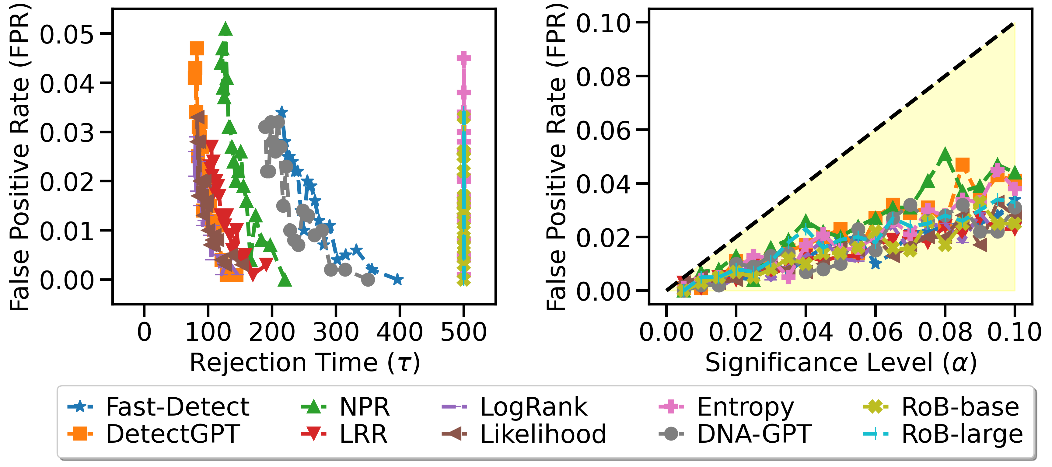
Results of Tests in Two Cases. Figure 5 and 6 show the results of detecting real Olympic news or news generated by Gemini-1.5-Flash , Gemini-1.5-Pro and PaLM 2 with designating human-written text from XSum dataset as in Scenario 1 and Scenario 2 respectively. In Scenario 1, our algorithm consistently controls the FPRs below the significance level for all source models, scoring models and score functions. It is because we used the real value between two sequences of human texts as , which satisfies the condition of , i.e., . This ensures that the wealth remains a supermartingale. Texts generated by PaLM 2 are detected almost immediately by most score functions within 100 time steps as illustrated in Figure 5(e) and Figure 5(f). Conversely, fake Olympic news generated by Gemini-1.5-Pro often fails to be identified as LLM-generated before 500 by some score functions, as shown in Figure 5(c) and Figure 5(d). Vertical lines in Figure 5(a)-5(d) are displayed because the the values for human texts and fake news, as shown in Table 1, are smaller than the corresponding values. This means that the score discrepancies between fake news and XSum texts do not exceed the threshold necessary for rejecting . Although under , the for Entropy when using Gemma-2B to score texts generated by Gemini-1.5-Pro is 0.2745, larger than the value of (), the discrepancy is too small to lead to a rejection of within 500 time steps.
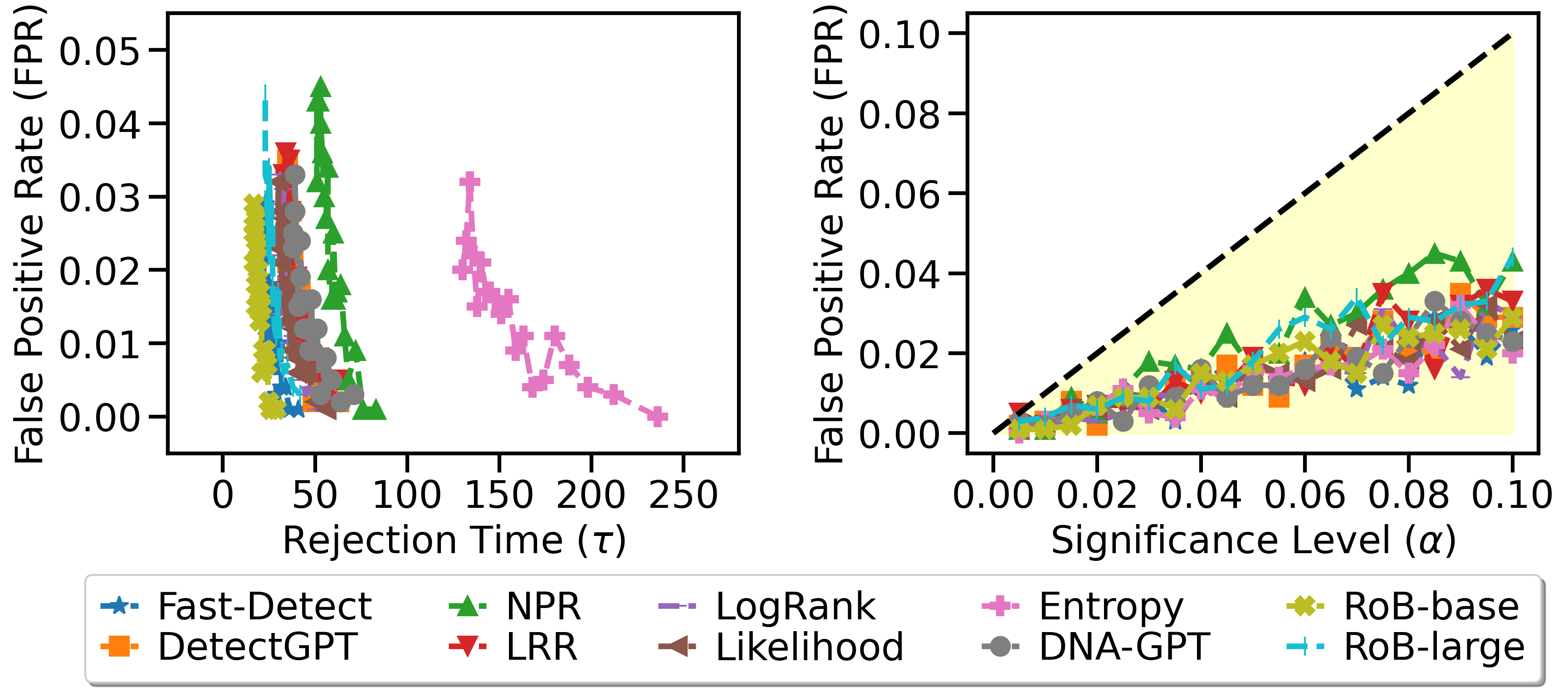
According to Figure 6, Scenario 2 exhibits a similar trend to that observed in Scenario 1, where texts generated by PaLM 2 are quickly declared as originating from an LLM, while texts produced by Gemini-1.5-Pro are identified more slowly. In Scenario 2, Fast-DetectGPT consistently outperforms all other score functions when using Neo-2.7 as scoring model, as evidenced by the results in Figure 6(a), 6(c) and 6(e). Only the score functions of supervised classifiers have FPRs slightly above the significance level . Although their average estimated values of in Table 5 are larger than the actual value under in Table 1, high FPRs often occur because most values estimated in 1000 repeated tests are smaller than the actual values. When using Gemma-2B as the scoring model in Scenario 2, four score functions: Fast-DetectGPT, LRR, Likelihood, and DNA-GPT consistently maintain FPRs within the expected range . Likelihood is the fastest to reject . However, estimated values of DetectGPT, NPR, and Entropy are smaller than real values under . Then, even when is true, the discrepancy between human texts exceed the estimated threshold for rejecting , which result in high FPRs, as shown in Figure 6(b), 6(d) and 6(f).
| Scoring Model | Score Function | XSum, Olympic | XSum, Olympic | XSum, Olympic | |||
|---|---|---|---|---|---|---|---|
| Human, | Human, | Human, | Human, | Human, | Human, | ||
| 1.5-Flash | Human | 1.5-Pro | Human | PaLM 2 | Human | ||
| Neo-2.7 | Fast-DetectGPT | 2.4786 | 0.3634 | 1.2992 | 0.3660 | 3.6338 | 0.4232 |
| DetectGPT | 0.3917 | 0.0202 | 0.3101 | 0.0274 | 0.6050 | 0.0052 | |
| NPR | 0.0232 | 0.0014 | 0.0155 | 0.0015 | 0.0398 | 0.0005 | |
| LRR | 0.1042 | 0.0324 | 0.0289 | 0.0328 | 0.2606 | 0.0370 | |
| Logrank | 0.2590 | 0.0543 | 0.1312 | 0.0561 | 0.4995 | 0.0743 | |
| Likelihood | 0.3882 | 0.0618 | 0.2170 | 0.0652 | 0.7641 | 0.0948 | |
| Entropy | 0.0481 | 0.0766 | 0.0067 | 0.0728 | 0.1878 | 0.0483 | |
| DNA-GPT | 0.1937 | 0.0968 | 0.0957 | 0.1032 | 0.4086 | 0.1083 | |
| \hdashline | RoBERTa-base | 0.2265 | 0.0461 | 0.0287 | 0.0491 | 0.6343 | 0.0370 |
| RoBERTa-large | 0.0885 | 0.0240 | 0.0249 | 0.0250 | 0.4197 | 0.0281 | |
| Gemma-2B | Fast-DetectGPT | 2.1412 | 0.5889 | 0.9321 | 0.5977 | 3.7314 | 0.6758 |
| DetectGPT | 0.7146 | 0.3538 | 0.6193 | 0.3530 | 0.8403 | 0.3360 | |
| NPR | 0.0632 | 0.0254 | 0.0477 | 0.0249 | 0.1005 | 0.0232 | |
| LRR | 0.1604 | 0.0129 | 0.0825 | 0.0112 | 0.3810 | 0.0038 | |
| Logrank | 0.3702 | 0.0973 | 0.2527 | 0.0932 | 0.5917 | 0.0687 | |
| Likelihood | 0.6093 | 0.1832 | 0.4276 | 0.1761 | 0.9705 | 0.1358 | |
| Entropy | 0.2668 | 0.2743 | 0.2745 | 0.2690 | 0.4543 | 0.2347 | |
| DNA-GPT | 0.2279 | 0.0353 | 0.1144 | 0.0491 | 0.4072 | 0.0681 | |
| \hdashline | RoBERTa-base | 0.2265 | 0.0461 | 0.0287 | 0.0491 | 0.6343 | 0.0370 |
| RoBERTa-large | 0.0885 | 0.0240 | 0.0249 | 0.0250 | 0.4197 | 0.0281 | |
| Scoring Model | Score Function | XSum, Olympic | XSum, Olympic | XSum, Olympic | |||
|---|---|---|---|---|---|---|---|
| Human, | Human, | Human, | Human, | Human, | Human, | ||
| 1.5-Flash | Human | 1.5-Pro | Human | PaLM 2 | Human | ||
| Neo-2.7 | Fast-DetectGPT | 7.6444 | 5.9956 | 6.5104 | 6.1546 | 9.1603 | 5.8870 |
| DetectGPT | 2.3985 | 2.3102 | 2.1416 | 2.2683 | 2.6095 | 2.7447 | |
| NPR | 0.1500 | 0.1436 | 0.1295 | 0.1465 | 0.1975 | 0.1353 | |
| LRR | 0.8129 | 0.5877 | 0.6400 | 0.5875 | 0.9793 | 0.5421 | |
| Logrank | 1.5861 | 1.6355 | 1.4065 | 1.6355 | 1.7298 | 1.6355 | |
| Likelihood | 2.3004 | 2.4540 | 1.9491 | 2.4540 | 2.6607 | 2.5559 | |
| Entropy | 1.6523 | 1.6630 | 1.5890 | 1.6702 | 1.9538 | 1.6265 | |
| DNA-GPT | 1.5063 | 1.5425 | 1.3621 | 1.5649 | 1.5455 | 1.6348 | |
| \hdashline | RoBERTa-base | 0.9997 | 0.9995 | 0.9995 | 0.9995 | 0.9997 | 0.9996 |
| RoBERTa-large | 0.9983 | 0.9856 | 0.8945 | 0.8945 | 0.9992 | 0.8608 | |
| Gemma-2B | Fast-DetectGPT | 7.7651 | 6.5619 | 7.3119 | 6.4343 | 8.6156 | 6.5640 |
| DetectGPT | 2.9905 | 2.5449 | 2.3846 | 2.4274 | 2.6807 | 2.7878 | |
| NPR | 0.3357 | 0.2196 | 0.3552 | 0.2318 | 0.4118 | 0.2403 | |
| LRR | 1.1189 | 0.7123 | 0.8780 | 0.7109 | 1.2897 | 0.7717 | |
| Logrank | 1.5731 | 1.6467 | 1.4713 | 1.6468 | 1.7538 | 1.6397 | |
| Likelihood | 2.4934 | 2.4229 | 2.3944 | 2.4228 | 2.8379 | 2.4694 | |
| Entropy | 1.9791 | 1.9117 | 1.8572 | 1.8854 | 2.1359 | 1.9210 | |
| DNA-GPT | 1.3214 | 1.4808 | 1.2891 | 1.4607 | 1.5014 | 1.6296 | |
| \hdashline | RoBERTa-base | 0.9997 | 0.9995 | 0.9995 | 0.9995 | 0.9997 | 0.9996 |
| RoBERTa-large | 0.9983 | 0.9856 | 0.8945 | 0.8945 | 0.9992 | 0.8608 | |
To summarize, the FPRs can be controlled below the significance level if the preset is greater than or equal to the actual absolute difference in mean scores between two sequences of human texts. However, if is greater than or is nearly equal to the value for human text and machine-generated text , it would be challenging for our algorithm to declare the source of as an LLM within a limited number of time steps under .
Moreover, we found that the rejection time is related to the relative magnitude of and . According to the definition of nonnegative wealth or , large within the range will result in large wealth which allows to quickly reach the threshold for wealth to correctly declare the unknown source as an LLM. Based on the previous proposition of the expected time upper bound for composite hypothesis, we guess that the actual rejection time in our experiment is probably related to the relative magnitude of and , where is a certain value for any in each test as shown in Table 2. We define the relative magnitude as and sort the score functions by this ratio from largest to smallest for Scenario 1, as displayed in the Rank column in Table 3. This ranking roughly corresponds to the chronological order of rejection shown in in Figure 5. The quick declaration of an LLM source when is generated by PaLM 2 and the slower rejection of when is generated by Gemini-1.5-Pro in Figure 5 can thus be attributed to the relatively larger and smaller values of , respectively. The negative ratios attributes to the reason that , which result in the vertical lines in figures. Similarly, we also show the values of for Scenario 2 as shown in Table 4, the conclusions in Scenario 1 still holds true for Scenario 2.
Thus, we prefer a larger discrepancy between scores of human-written texts and machine-generated texts, which can increase . Furthermore, a smaller variation among scores of texts from the same source can reduce . These properties facilitate a shorter rejection time under .
| Scoring Model | Score Function | Human, 1.5-Flash | Human, 1.5-Pro | Human, PaLM 2 | |||
|---|---|---|---|---|---|---|---|
| Ratio | Rank | Ratio | Rank | Ratio | Rank | ||
| Neo-2.7 | Fast-DetectGPT | 0.2905 | 1 | 0.1519 | 1 | 0.3675 | 3 |
| DetectGPT | 0.1562 | 3 | 0.1337 | 2 | 0.2303 | 7 | |
| NPR | 0.1467 | 4 | 0.1093 | 3 | 0.1995 | 9 | |
| LRR | 0.0920 | 7 | -0.0064 | 8 | 0.2373 | 6 | |
| Logrank | 0.1336 | 6 | 0.0556 | 5 | 0.2568 | 5 | |
| Likelihood | 0.1458 | 5 | 0.0806 | 4 | 0.2608 | 4 | |
| Entropy | -0.0181 | 10 | -0.0436 | 10 | 0.0732 | 10 | |
| DNA-GPT | 0.0687 | 8 | -0.0060 | 7 | 0.2089 | 8 | |
| \hdashline | RoBERTa-base | 0.1892 | 2 | -0.0215 | 9 | 0.6205 | 1 |
| RoBERTa-large | 0.0662 | 9 | -0.0001 | 6 | 0.4032 | 2 | |
| Gemma-2B | Fast-DetectGPT | 0.2163 | 1 | 0.0498 | 7 | 0.3848 | 3 |
| DetectGPT | 0.1368 | 6 | 0.1311 | 1 | 0.2151 | 8 | |
| NPR | 0.1218 | 8 | 0.0690 | 5 | 0.1989 | 9 | |
| LRR | 0.1334 | 7 | 0.0823 | 4 | 0.2933 | 6 | |
| Logrank | 0.1849 | 3 | 0.1157 | 2 | 0.3104 | 4 | |
| Likelihood | 0.1844 | 4 | 0.1134 | 3 | 0.3089 | 5 | |
| Entropy | -0.0044 | 10 | 0.0035 | 8 | 0.1155 | 10 | |
| DNA-GPT | 0.1498 | 5 | 0.0527 | 6 | 0.2366 | 7 | |
| \hdashline | RoBERTa-base | 0.1892 | 2 | -0.0215 | 10 | 0.6205 | 1 |
| RoBERTa-large | 0.0662 | 9 | -0.0001 | 9 | 0.4032 | 2 | |
| Scoring Model | Score Function | Human, 1.5-Flash | Human, 1.5-Pro | Human, PaLM 2 | |||
|---|---|---|---|---|---|---|---|
| Ratio | Rank | Ratio | Rank | Ratio | Rank | ||
| Neo-2.7 | Fast-DetectGPT | 0.1895 | 1 | 0.0874 | 1 | 0.2420 | 2 |
| DetectGPT | 0.0427 | 7 | 0.0103 | 2 | 0.1024 | 9 | |
| NPR | 0.0592 | 2 | 0.0076 | 3 | 0.1268 | 8 | |
| LRR | 0.0474 | 5 | -0.0653 | 7 | 0.1568 | 7 | |
| Logrank | 0.0576 | 4 | -0.0218 | 5 | 0.1687 | 4 | |
| Likelihood | 0.0582 | 3 | -0.0132 | 4 | 0.1680 | 5 | |
| Entropy | -0.0883 | 10 | -0.1162 | 10 | -0.0051 | 10 | |
| DNA-GPT | 0.0405 | 8 | -0.0298 | 6 | 0.1636 | 6 | |
| \hdashline | RoBERTa-base | 0.0461 | 6 | -0.1042 | 9 | 0.2713 | 1 |
| RoBERTa-large | 0.0092 | 9 | -0.0942 | 8 | 0.1814 | 3 | |
| Gemma-2B | Fast-DetectGPT | 0.1562 | 1 | 0.0368 | 5 | 0.2444 | 2 |
| DetectGPT | 0.1351 | 3 | 0.1147 | 2 | 0.1552 | 8 | |
| NPR | 0.1492 | 2 | 0.1167 | 1 | 0.1961 | 6 | |
| LRR | 0.0867 | 6 | 0.0117 | 7 | 0.1959 | 5 | |
| Logrank | 0.1205 | 5 | 0.0607 | 4 | 0.2086 | 4 | |
| Likelihood | 0.1267 | 4 | 0.0702 | 3 | 0.2144 | 3 | |
| Entropy | 0.0270 | 9 | 0.0293 | 6 | 0.1017 | 10 | |
| DNA-GPT | 0.0713 | 7 | -0.0144 | 8 | 0.1747 | 9 | |
| \hdashline | RoBERTa-base | 0.0462 | 8 | -0.1007 | 9 | 0.2737 | 1 |
| RoBERTa-large | 0.0060 | 10 | -0.1013 1 | 0 | 0.1803 | 7 | |
| Scoring Model | Score Function | XSum, Olympic | XSum, Olympic | XSum, Olympic | |||
|---|---|---|---|---|---|---|---|
| Human, | Human, | Human, | Human, | Human, | Human, | ||
| 1.5-Flash | Human | 1.5-Pro | Human | PaLM 2 | Human | ||
| Neo-2.7 | Fast-DetectGPT | 0.6357 | 0.6371 | 0.6395 | 0.6417 | 0.6415 | 0.6426 |
| DetectGPT | 0.2781 | 0.2807 | 0.2840 | 0.2870 | 0.2851 | 0.2847 | |
| NPR | 0.0141 | 0.0141 | 0.0145 | 0.0146 | 0.0140 | 0.0141 | |
| LRR | 0.0665 | 0.0666 | 0.0674 | 0.0676 | 0.0652 | 0.0649 | |
| Logrank | 0.1634 | 0.1632 | 0.1624 | 0.1624 | 0.1597 | 0.1590 | |
| Likelihood | 0.2448 | 0.2450 | 0.2455 | 0.2426 | 0.2419 | 0.2416 | |
| Entropy | 0.1994 | 0.1978 | 0.2022 | 0.2000 | 0.1973 | 0.2004 | |
| DNA-GPT | 0.1404 | 0.1394 | 0.1321 | 0.1314 | 0.1345 | 0.1320 | |
| \hdashline | RoBERTa-base | 0.1438 | 0.1459 | 0.1463 | 0.1496 | 0.1261 | 0.1206 |
| RoBERTa-large | 0.0768 | 0.0787 | 0.0732 | 0.0740 | 0.0821 | 0.0853 | |
| Gemma-2B | Fast-DetectGPT | 0.6806 | 0.6785 | 0.6749 | 0.6726 | 0.6781 | 0.6825 |
| DetectGPT | 0.2731 | 0.2725 | 0.2685 | 0.2664 | 0.2822 | 0.2840 | |
| NPR | 0.0170 | 0.0168 | 0.0171 | 0.0171 | 0.0169 | 0.0169 | |
| LRR | 0.0724 | 0.0728 | 0.0732 | 0.0735 | 0.0725 | 0.0719 | |
| Logrank | 0.1547 | 0.1542 | 0.1567 | 0.1550 | 0.1556 | 0.1521 | |
| Likelihood | 0.2438 | 0.2414 | 0.2472 | 0.2473 | 0.2427 | 0.2429 | |
| Entropy | 0.2082 | 0.2088 | 0.2120 | 0.2092 | 0.2076 | 0.2078 | |
| DNA-GPT | 0.1354 | 0.1355 | 0.1317 | 0.1325 | 0.1278 | 0.1286 | |
| \hdashline | RoBERTa-base | 0.1438 | 0.1433 | 0.1437 | 0.1448 | 0.1198 | 0.1208 |
| RoBERTa-large | 0.0807 | 0.0800 | 0.0750 | 0.0743 | 0.0831 | 0.0823 | |
| Scoring Model | Score Function | XSum, Olympic | XSum, Olympic | XSum, Olympic | |||
|---|---|---|---|---|---|---|---|
| Human, | Human, | Human, | Human, | Human, | Human, | ||
| 1.5-Flash | Human | 1.5-Pro | Human | PaLM 2 | Human | ||
| Neo-2.7 | Fast-DetectGPT | 10.3586 | 6.6788 | 8.1840 | 6.7517 | 13.0086 | 6.8456 |
| DetectGPT | 2.9396 | 2.6967 | 2.8232 | 2.7183 | 3.4076 | 2.7313 | |
| NPR | 0.1680 | 0.1358 | 0.1464 | 0.1397 | 0.2178 | 0.1337 | |
| LRR | 0.8620 | 0.6418 | 0.6572 | 0.6298 | 1.3115 | 0.6294 | |
| Logrank | 1.8230 | 1.6746 | 1.5966 | 1.6676 | 2.1740 | 1.6807 | |
| Likelihood | 2.7089 | 2.5370 | 2.4016 | 2.4975 | 3.3493 | 2.5529 | |
| Entropy | 1.9123 | 1.9560 | 1.8840 | 1.9841 | 2.0712 | 1.9249 | |
| DNA-GPT | 1.4570 | 1.5696 | 1.3530 | 1.5374 | 1.8097 | 1.6042 | |
| \hdashline | RoBERTa-base | 1.9404 | 1.1136 | 1.2745 | 1.1795 | 1.9993 | 1.0390 |
| RoBERTa-large | 1.3443 | 0.6548 | 0.5857 | 0.5713 | 1.9435 | 0.6014 | |
| Gemma-2B | Fast-DetectGPT | 10.0337 | 7.4171 | 7.6691 | 7.4983 | 13.1693 | 7.6051 |
| DetectGPT | 3.5422 | 3.0998 | 3.3271 | 3.0398 | 3.8780 | 3.1375 | |
| NPR | 0.3264 | 0.2326 | 0.2795 | 0.2346 | 0.4432 | 0.2270 | |
| LRR | 1.0874 | 0.7253 | 0.8615 | 0.7283 | 1.6474 | 0.7234 | |
| Logrank | 1.9435 | 1.6850 | 1.7377 | 1.6759 | 2.2468 | 1.6162 | |
| Likelihood | 3.1277 | 2.6890 | 2.8156 | 2.6686 | 3.6366 | 2.5868 | |
| Entropy | 2.3749 | 2.4105 | 2.3417 | 2.3869 | 2.6341 | 2.3166 | |
| DNA-GPT | 1.4319 | 1.3889 | 1.3308 | 1.3798 | 1.7274 | 1.4109 | |
| \hdashline | RoBERTa-base | 1.9343 | 1.1536 | 1.2867 | 1.1800 | 1.9993 | 0.9913 |
| RoBERTa-large | 1.3832 | 0.6636 | 0.5695 | 0.5501 | 1.9499 | 0.6488 | |
Based on the results, when we know the actual value of and , our algorithm is very effective. When we estimate their values based on the previous samples that we get, the algorithm can still exhibit a good performance for most score functions. It can be inferred that the rejection time and FPRs of Algorithm 1 are effected by the score function and the scoring model that we select for our algorithm. If the configuration can further amplify the score discrepancy between human-written texts and machine-generated texts, the rejection time can be shortened. If the the score discrepancy between human texts is small, the value FPR will be low.
Comparisons with the Baselines. Permutation test is a fixed-time test. Our goal is to test whether the source of text is the same as that of the human-written text , i.e., whether their scores are from the same distribution. If we choose the mean value as the test statistic, the null hypothesis is that the means are equal () with a batch size of k. Once we have generated samples from these two sources, we conduct the test. Under the assumption that is true, the samples are drawn from the same distribution, which means that the observed discrepancy between the two batches of scores is supposed to be minimal. The test determines whether this difference between the sample means is large enough to reject at a significance level. Specifically, we compare the p-value with the significance level: for each batch in an uncorrected test, and for the -th batch in a corrected test. The permutation test is conducted as below:
(1) Calculate the observed mean difference of these two batches, and assume that is true;
(2) Combine these two sequences into one dataset, reshuffle the data, and divide it into two new groups. This is the permutation operation. Calculate the sampled absolute mean difference for the -th permutation, ;
(5) Repeat step (2) for a sufficient number of permutations ( in our test);
(6) Calculate the p-value, which is the proportion of permutations where , relative to the total number of permutations (). If the p-value is greater than the significance level , we retain ; otherwise we reject .
Proceed to the next batch if is retained in this batch test, and continue the above process until is rejected or all data are tested.
In the experiment, we consider the composite hypothesis testing, which means the null hypothesis is . If we still use the above permutation test, it will become much easier for to hold, even when is actually true. This would result in significantly higher FPRs. Thus, we only check p-values when the observed exceeds the estimated . The rejection time and FPR that we plot are the average values across 1000 repeated runs for each significance level.
Permutation test is very time-consuming, because if we have m samples for each group, then we will get m/k batches, each batch need to conduct the above steps.
As observed in Figure 7, the permutation tests without correction always have higher FPRs under than that with corrected significance levels. This phenomenon aligns with the fact that without significance level adjustments, it is impossible to control the type-I error. Permutation tests with large batch sizes demonstrate relatively low FPRs, which are approximate equal to 0. However, this seemingly excellent performance is due to the fact that the preset values are much larger than the actual absolute difference in mean scores between sequences of XSum texts and 2024 Olympic news. This discrepancy results in fewer or no p-value checks, thus sustaining . Consequently, the FPRs are nearly identical across each significance level . Permutation tests are sensitive to the discrepancies between two sequences, and the value tends to change more with smaller batch sizes due to variation among scores of texts from the same source. Although a permutation test can reject after the first batch test, it consistently exhibit an FPR greater than . Moreover, even if we set the value of based on a much larger sample size, rather than from estimates derived from a few points, there will still be variance between the value calculated in batches and the preset . As long as calculated by a batch of samples is greater than the preset , the permutation test is likely to have a large FPR under . Compared to fixed-time methods, our method can use parameter estimates based on just a few points to ensure faster rejection and lower FPRs. It can save time with high acuuracy especially when there is no prior knowledge of the threshold for composite hypotheses.
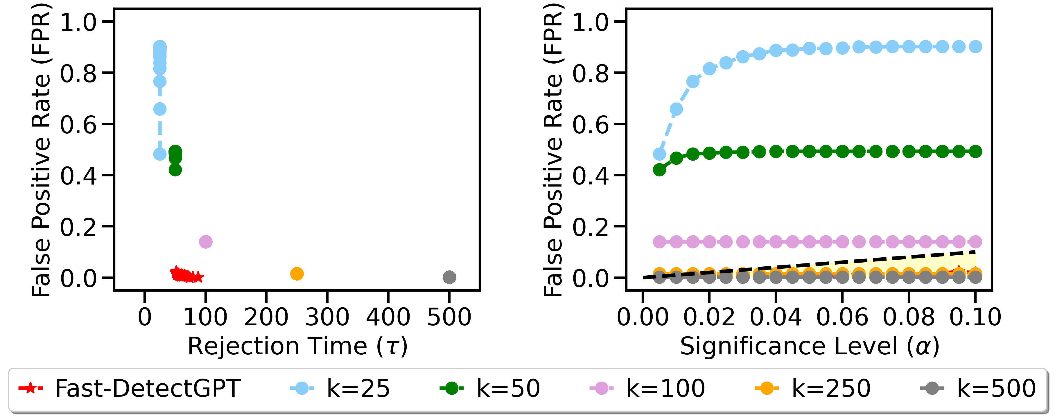
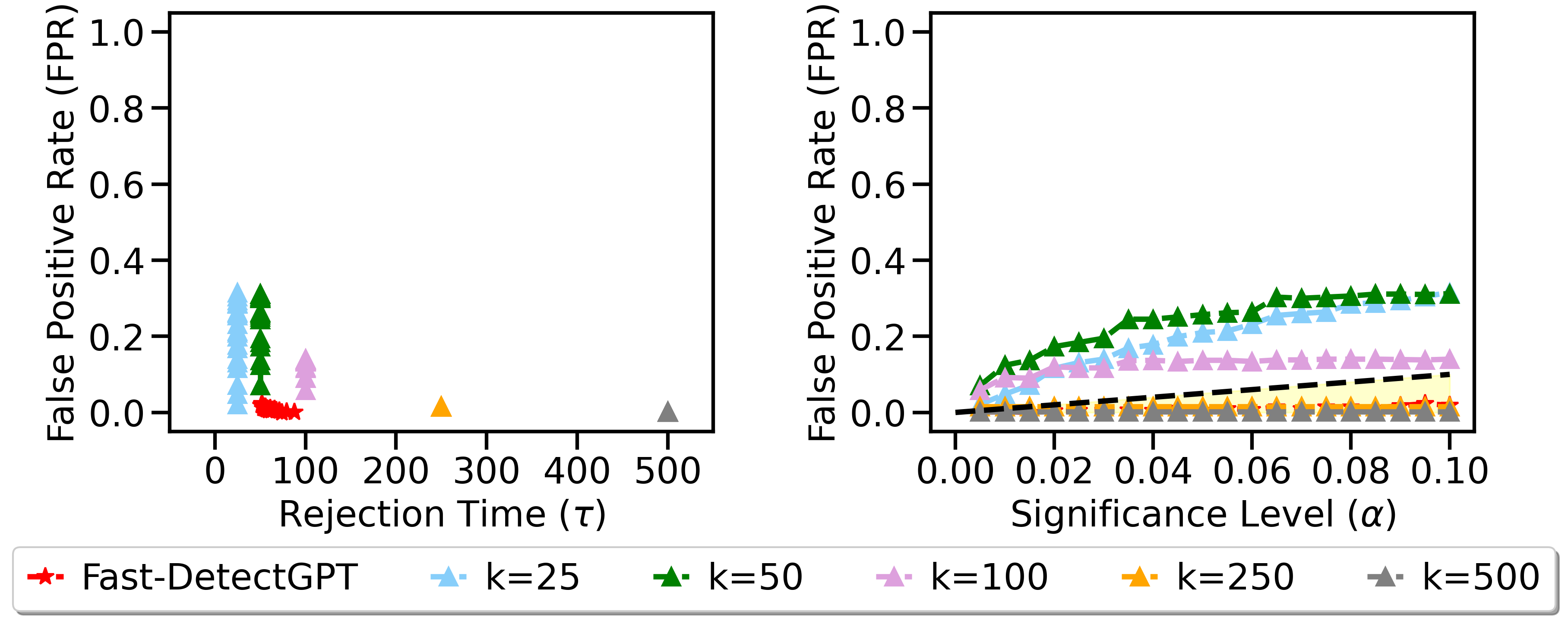
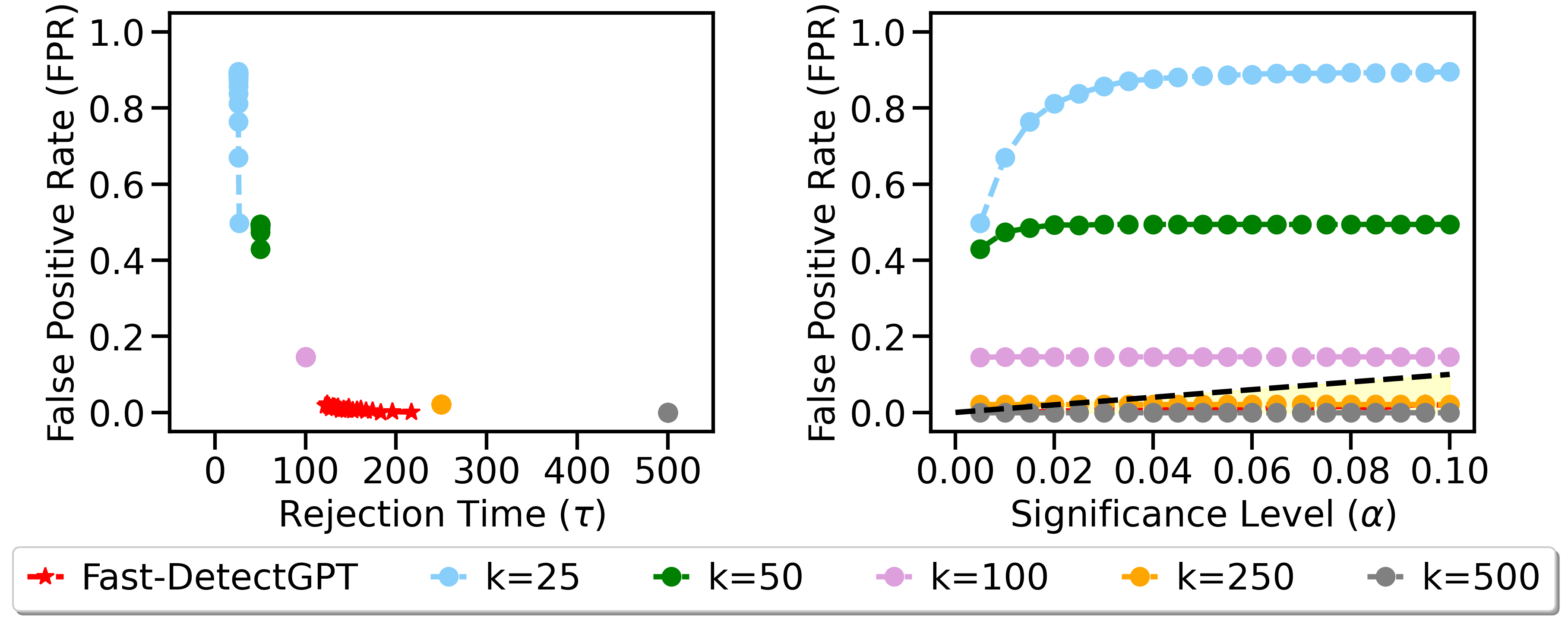
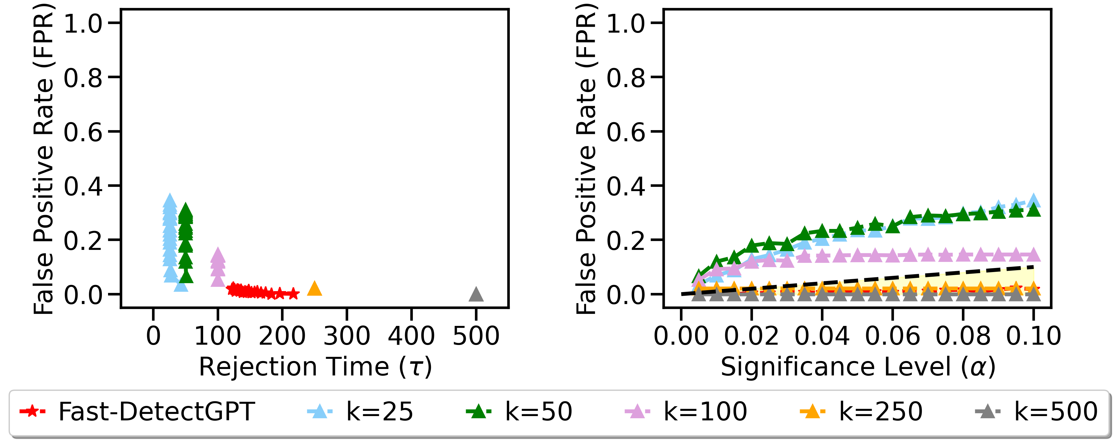
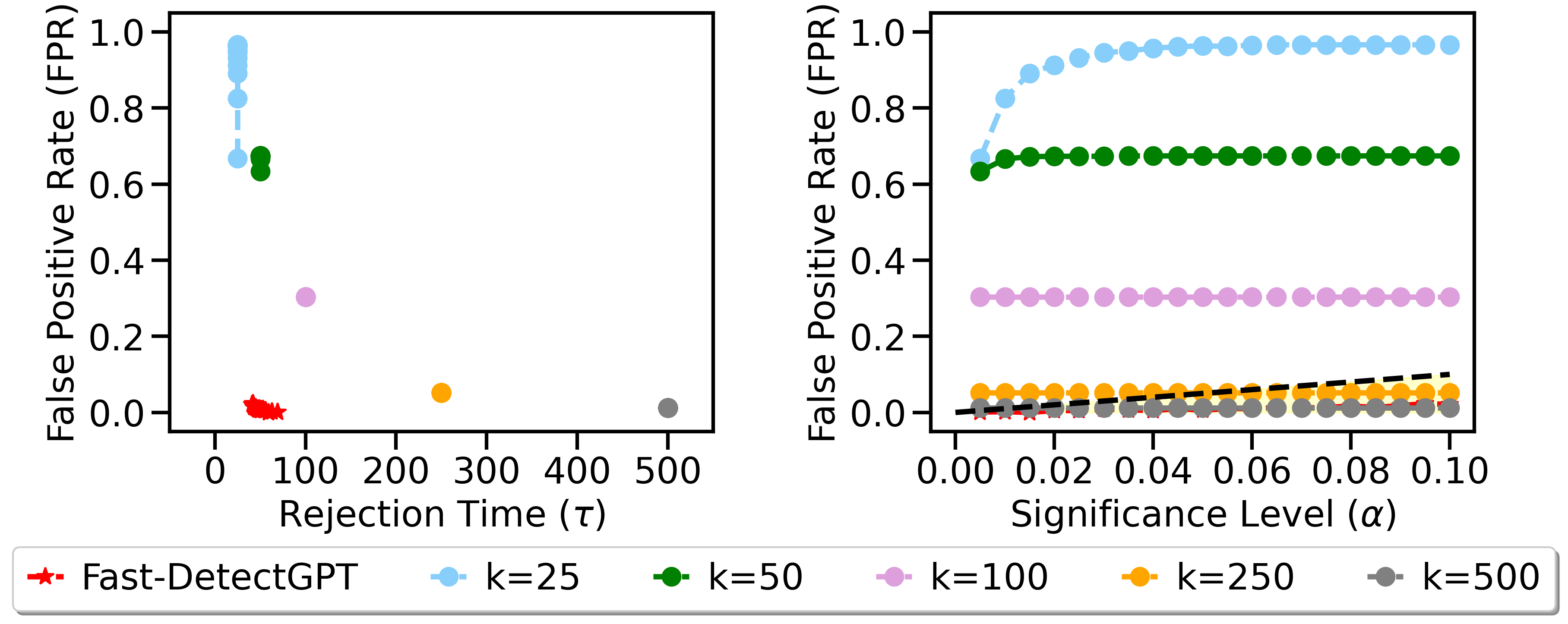
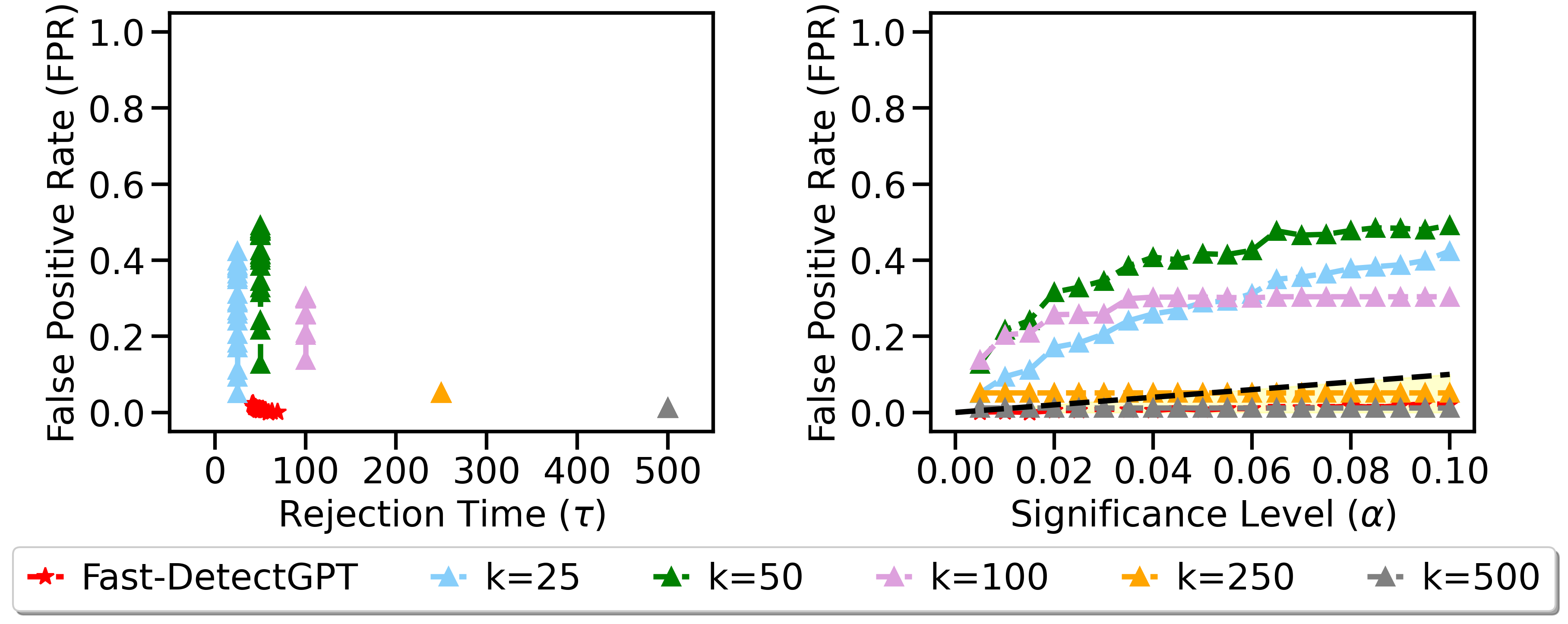
Appendix H Experiment Results of detecting texts from three domains
We also test on the dataset of Bao et al. [2023] to explore the influence of text domains on the detection result of our algorithm. In this experiment, we only consider Scenario 1. We let be human-written text from three datasets following Mitchell et al. [2023], each chosen to represent a typical LLMs application scenario. Specifically, we incorporate news articles sourced from the XSum dataset[Narayan et al., 2018], stories from Reddit WritingPrompts dataset[Fan et al., 2018] and long-form answers written by human experts from the PubMedQA dataset[Jin et al., 2019]. Then, the capability of our algorithm is evaluated by detecting the source of texts originated from the above source models or human datasets. Source models involved in this experiment are GPT-3 [Brown, 2020], ChatGPT [OpenAI, 2022], and GPT-4 [Achiam et al., 2023] while the scoring model is Neo-2.7[Black et al., 2021]. The perturbation function for DetectGPT and NPR is T5-11B, and the sampling model for Fast-DetectGPT is GPT-J-6B.
Figure 8(a) and Figure 8(b) show the averaged results when two streams of texts are from the same domain and different domains respectively, i.e., both sequences of texts are sampled from/prompted according to the same dataset/different datasets. Specifically, we get the results by averaging rejection time and FPR under each -significance level across the corresponding results of three LLMs (GPT-3, ChatGPT, GPT-4) and three same/different domain settings shown in Figure 10 and 8(b). After comparing these two figures, we find that the correct declaration of an LLM source happens more quickly when the prepared texts and the texts to be detected are from the same domain. Our algorithm can control FPRs below the significance level for all score functions while the averaged rejection times for them are all shorter than 150. Among all functions, Fast-DetectGPT is the fastest to reject , with average value of being around 40 for same-domain texts and about 80 for different-domain texts.
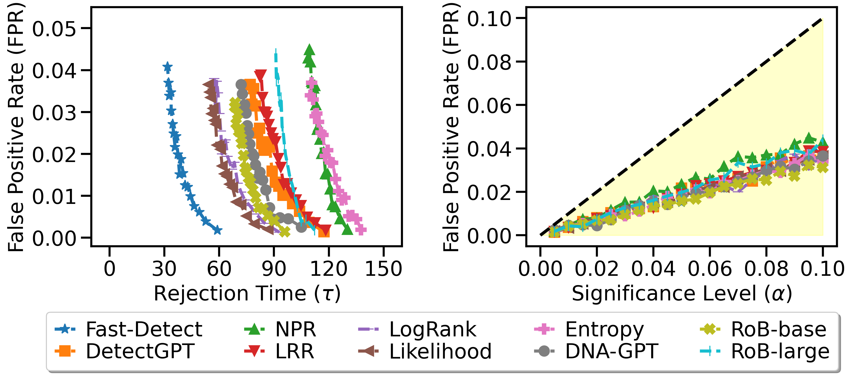
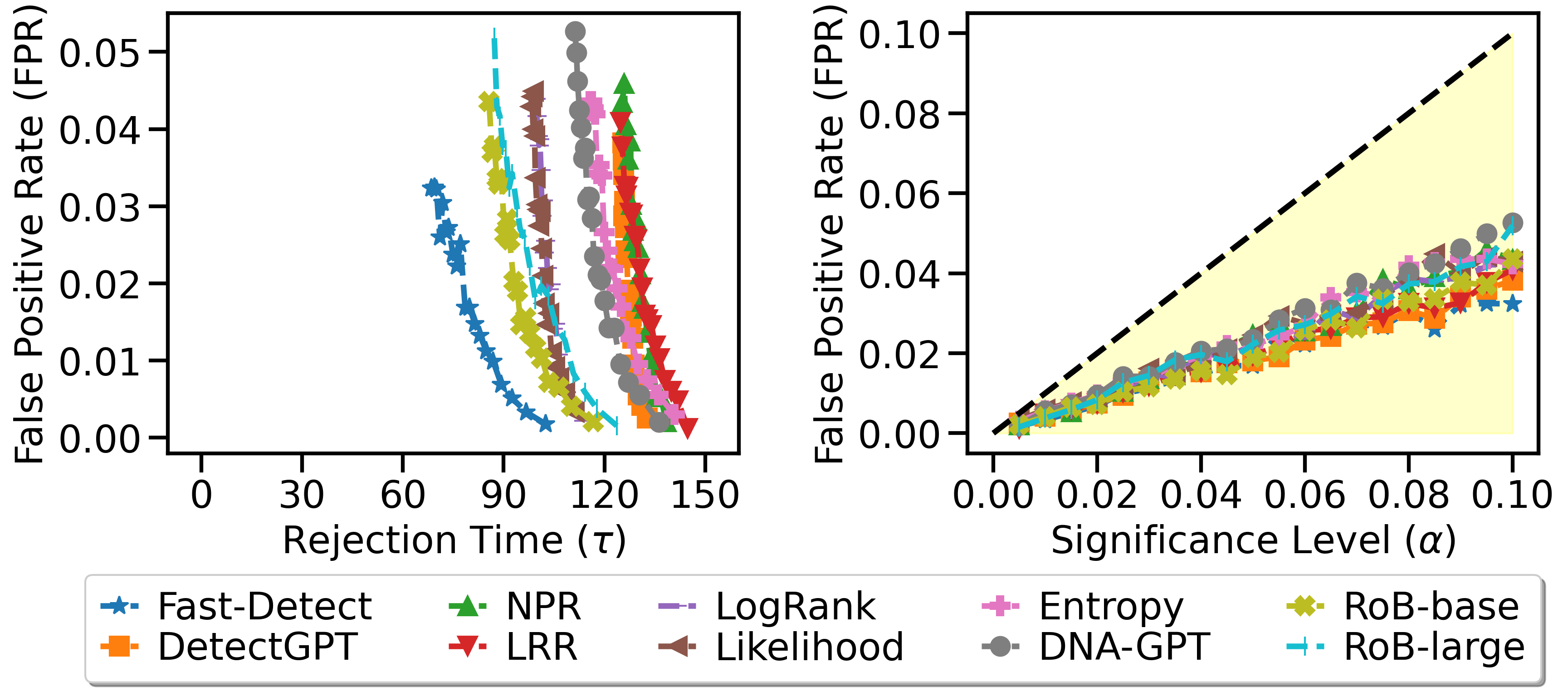
Specifically, according to Figure 10 , when texts are both sampled from PubMedQA datasets, the behaviour of most score functions are worse than that for texts from XSum and WritingPrompts. Specifically, it costs more time for them to reject . There are more vertical lines in Figure 9(c), 10(i) and 9(i), which means texts generated by GPT-4 are more challenging for our algorithm when using certain score functions such as RoBERTa-base/large to detect before .
Figure 8(b) illustrates the performance of our algorithm with different score functions when detecting two streams of different-domain texts. All functions can guarantee FPRs below the -significance level. When is from XSum and is generated by GPT-4 based on Writing, only Fast-DetectGPT can declare the source of as an LLM before . Another interesting phenomenon is that when is generated by GPT-3 based on PubMed, tests with most score functions fail to successfully identify its source as an LLM before the time budget expires, regardless of the domain of the human text used as for detection. Only the score functions of two supervised classifiers consistently reject before , which is shown as Figure 9(g), 10(d) and 10(g).
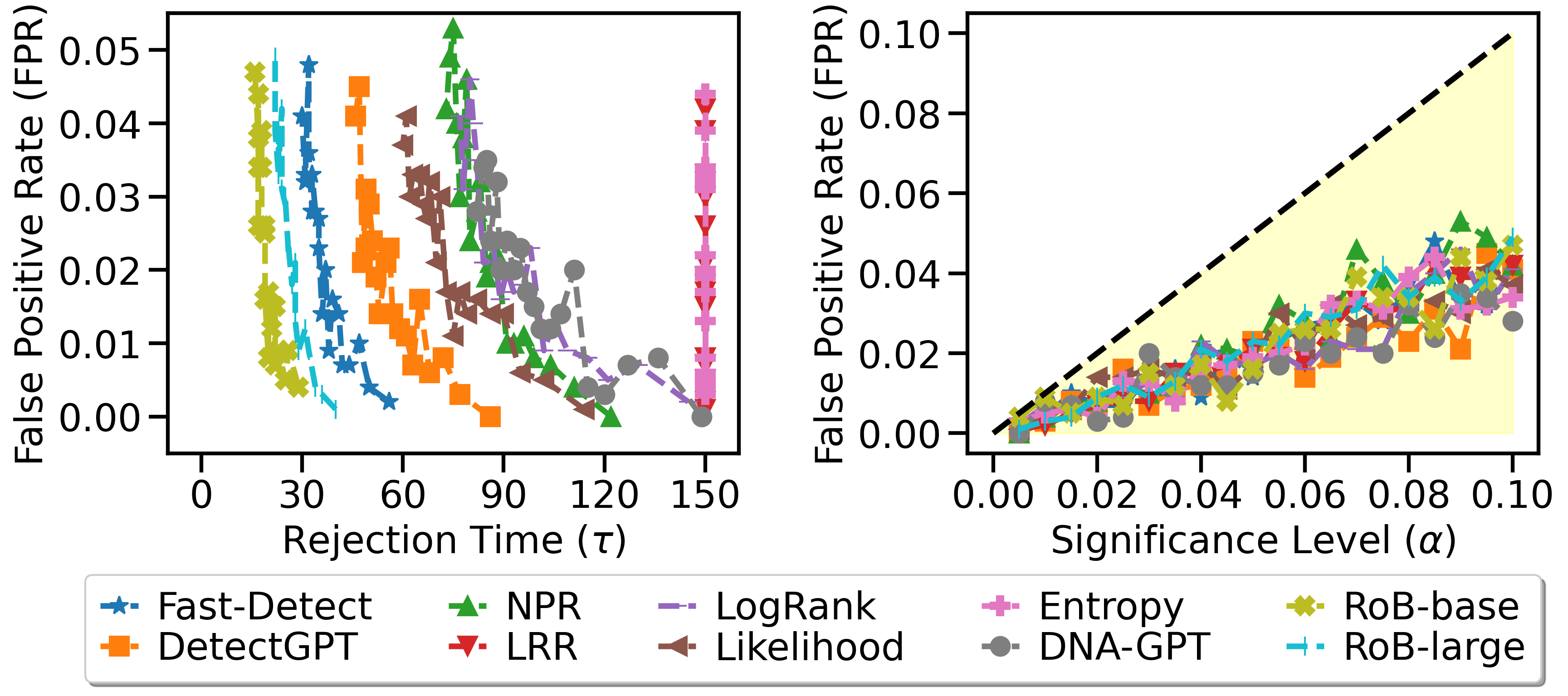
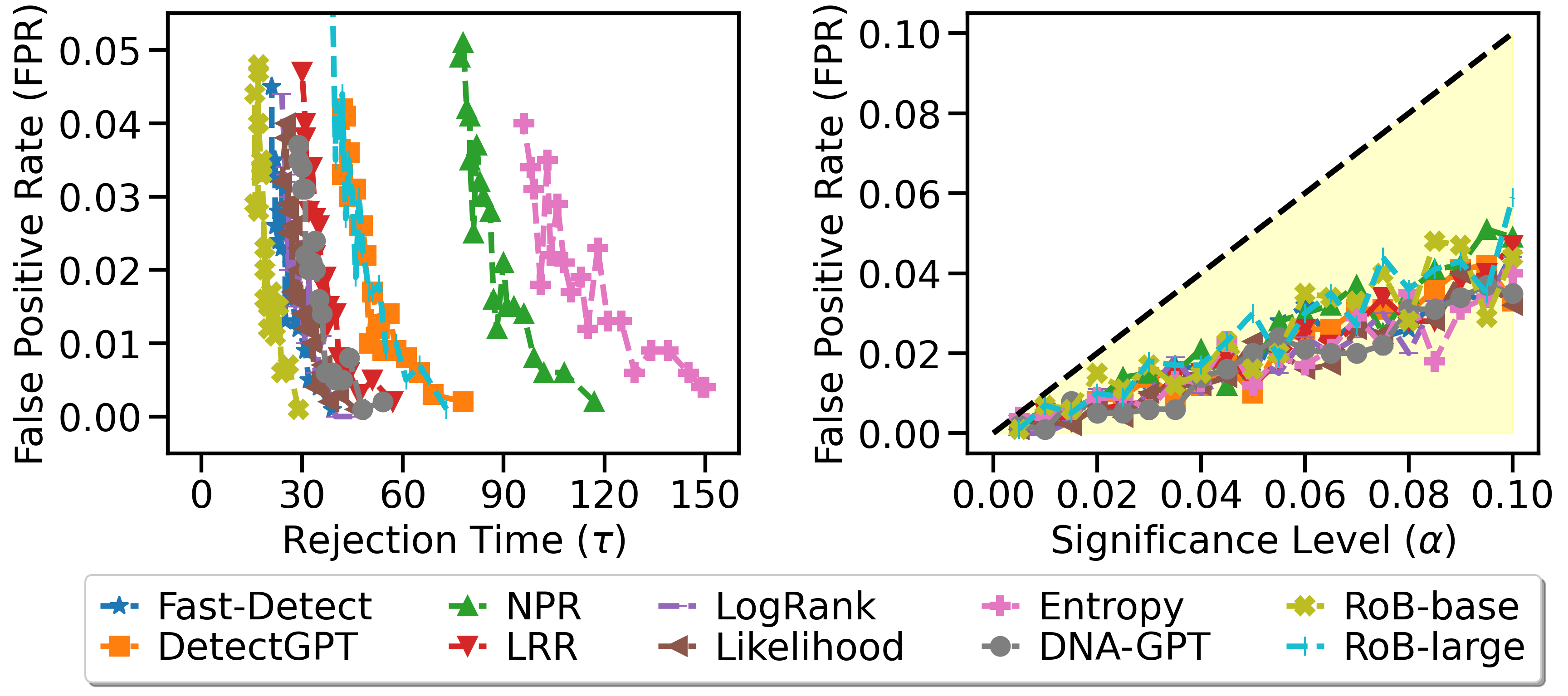
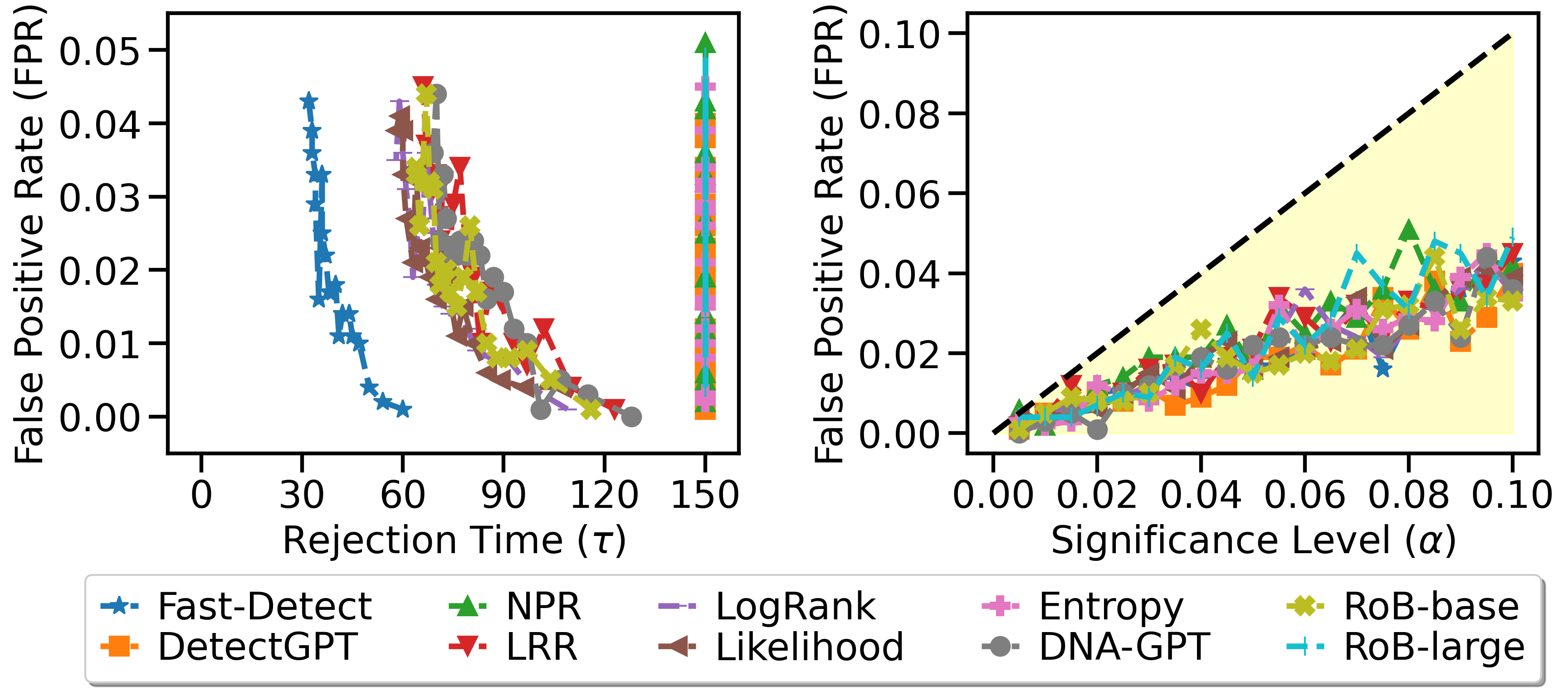
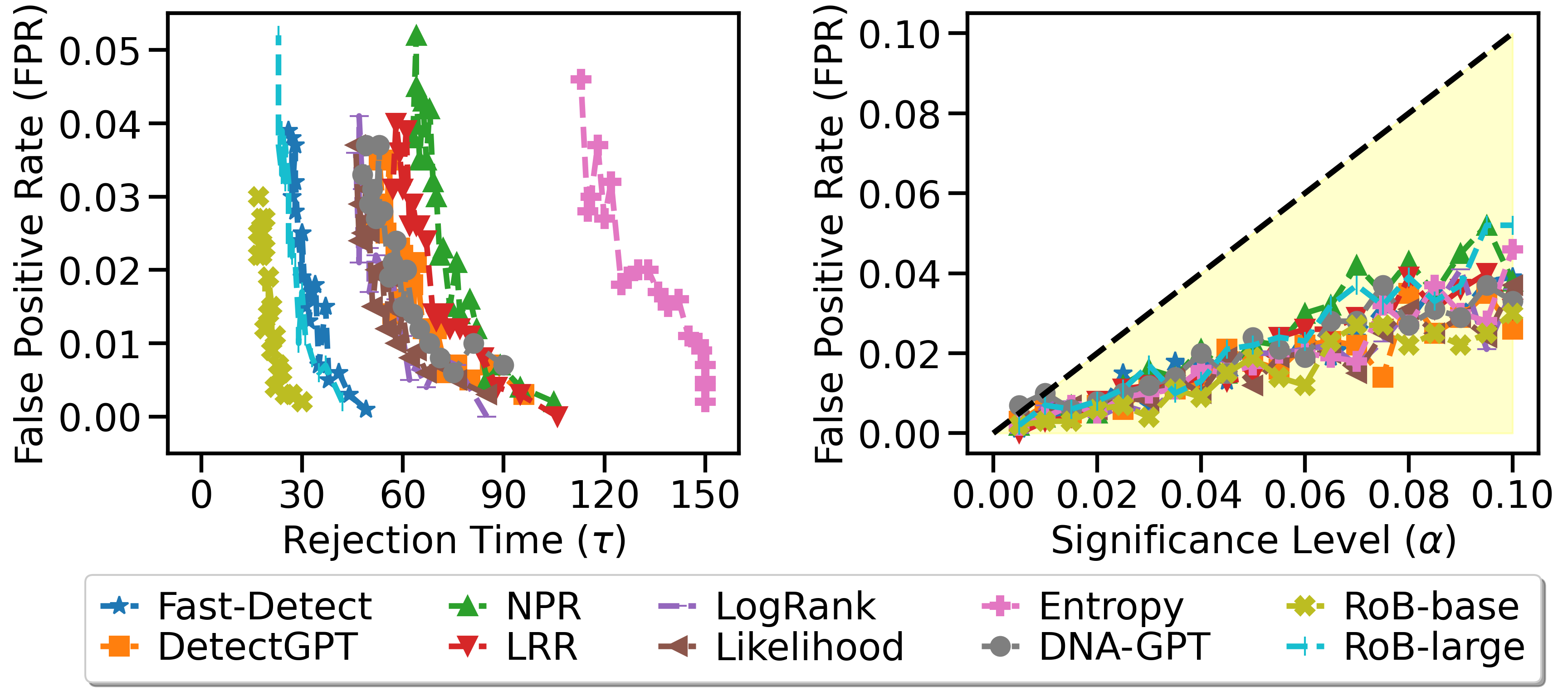
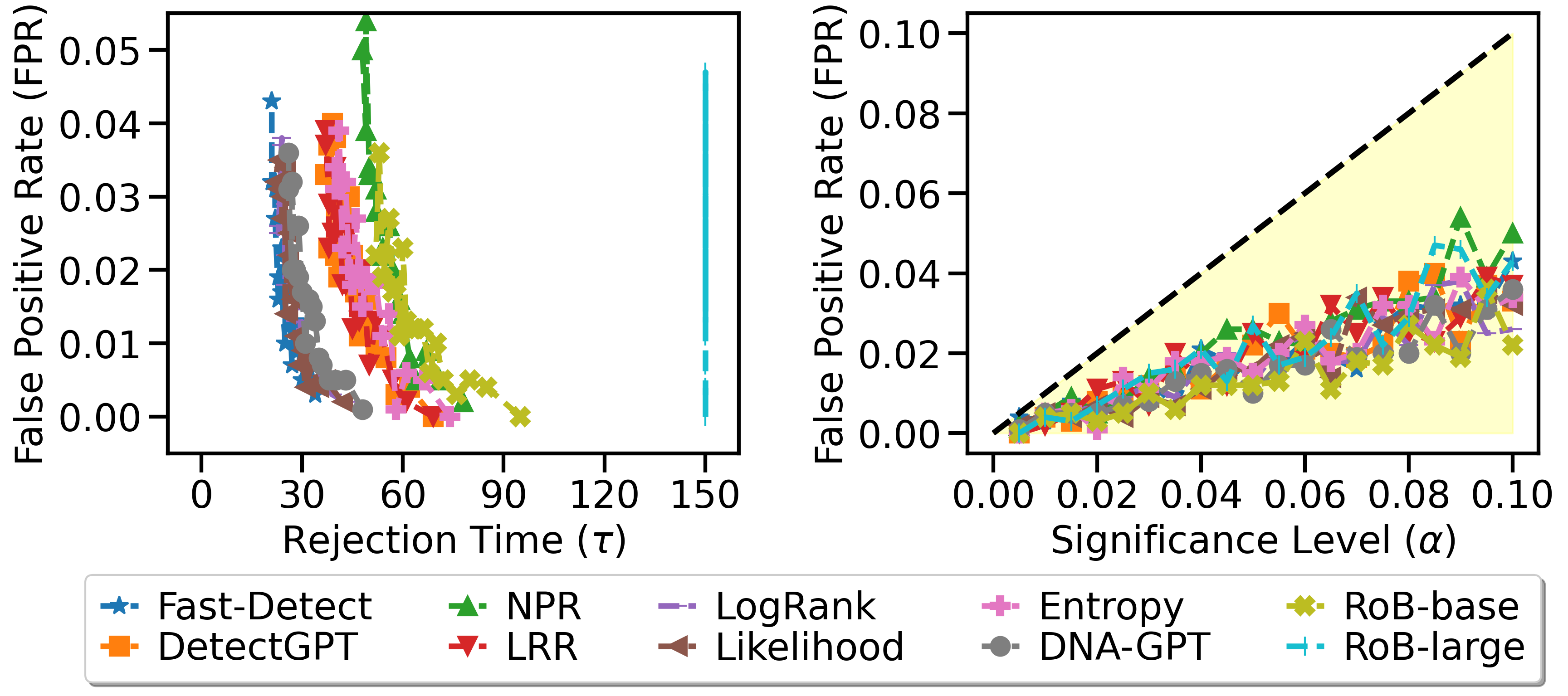
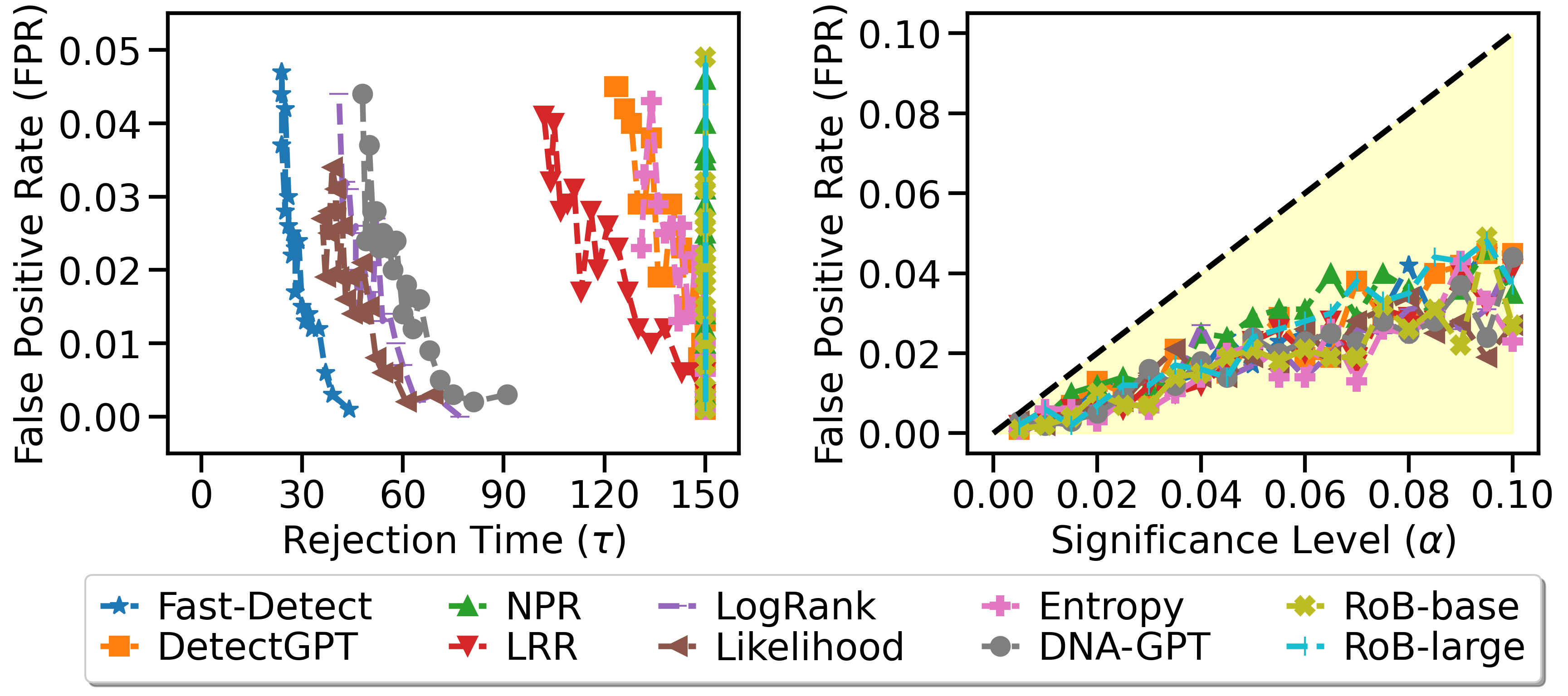
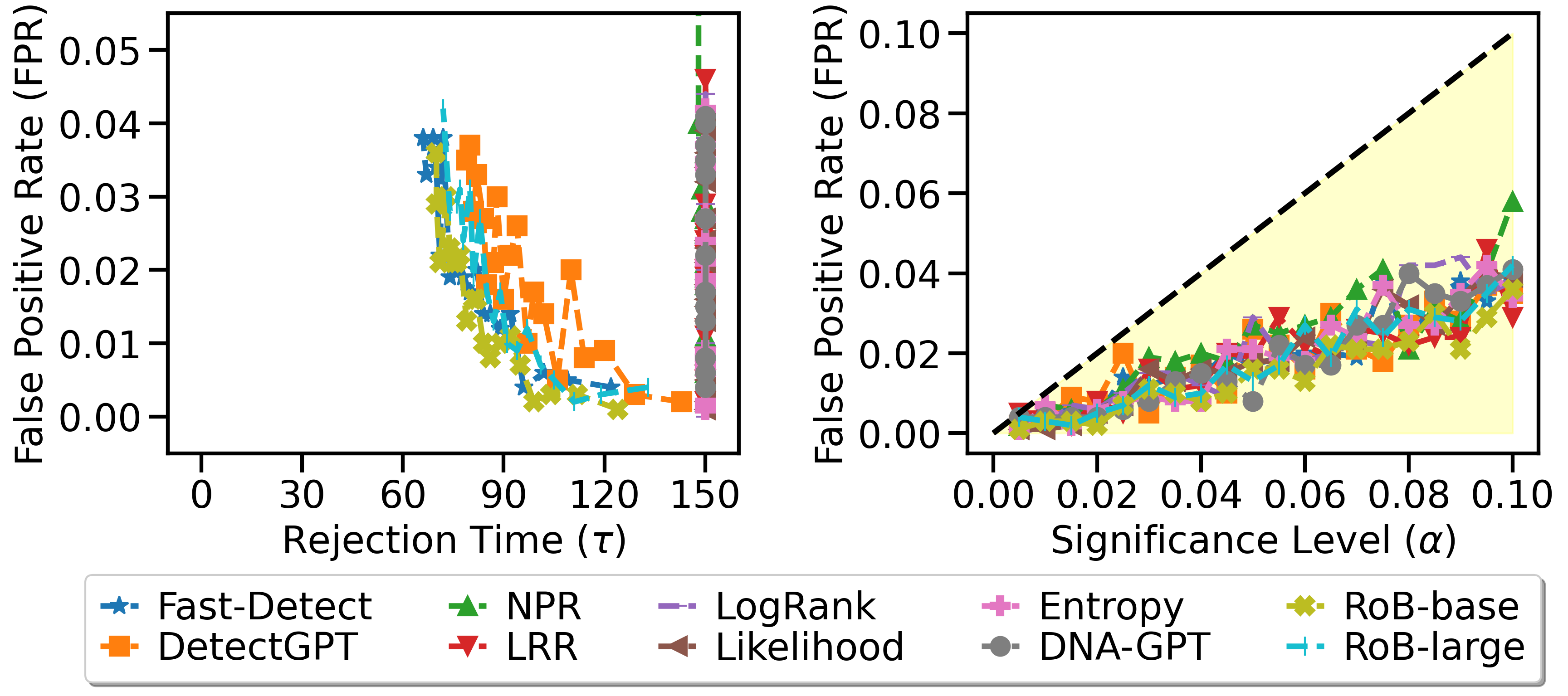
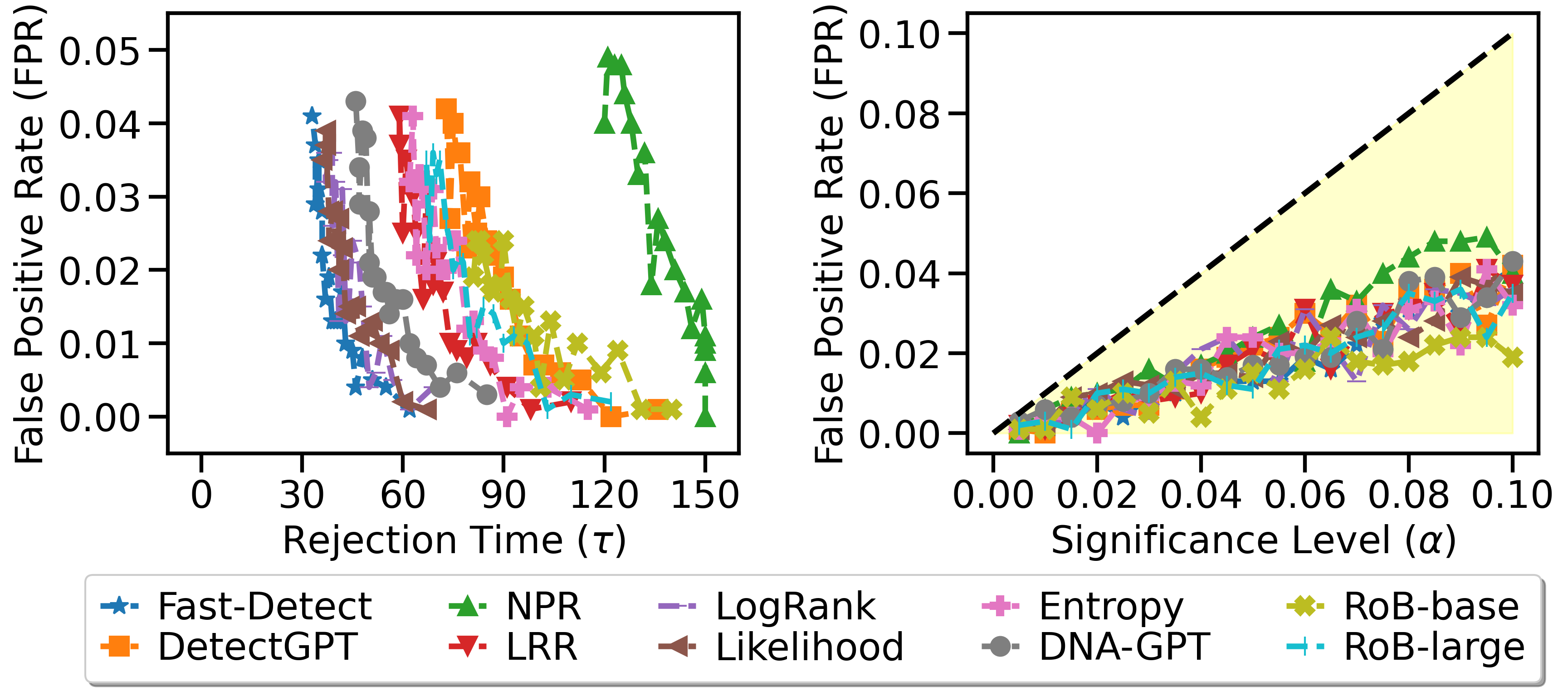
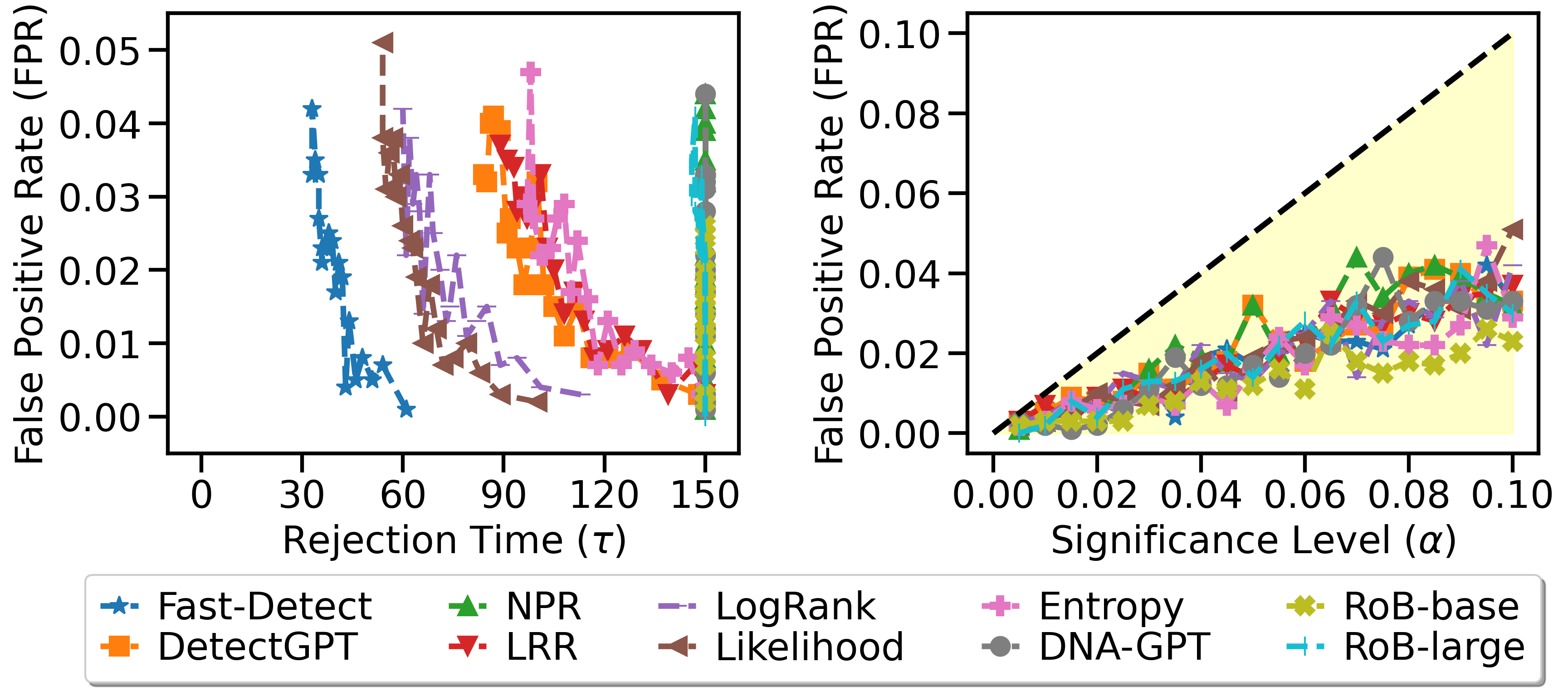
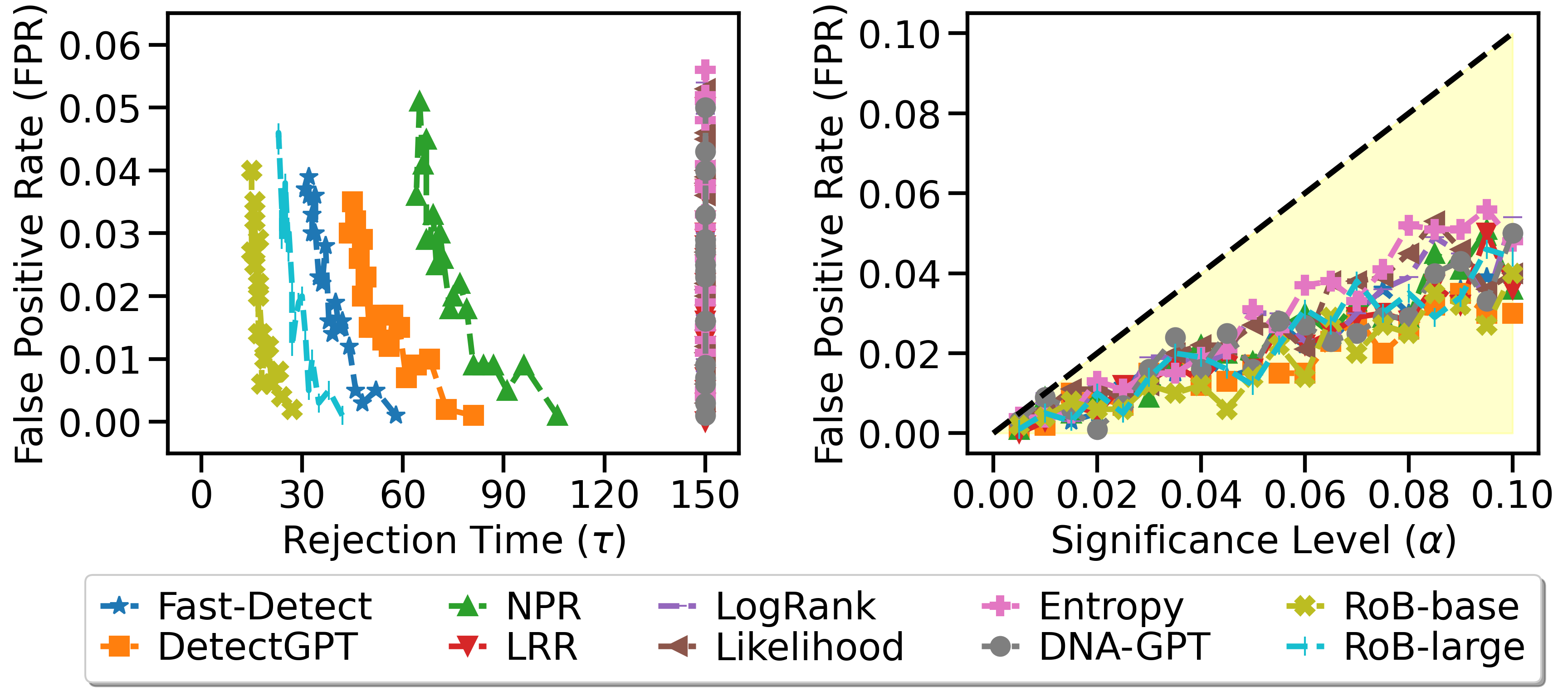
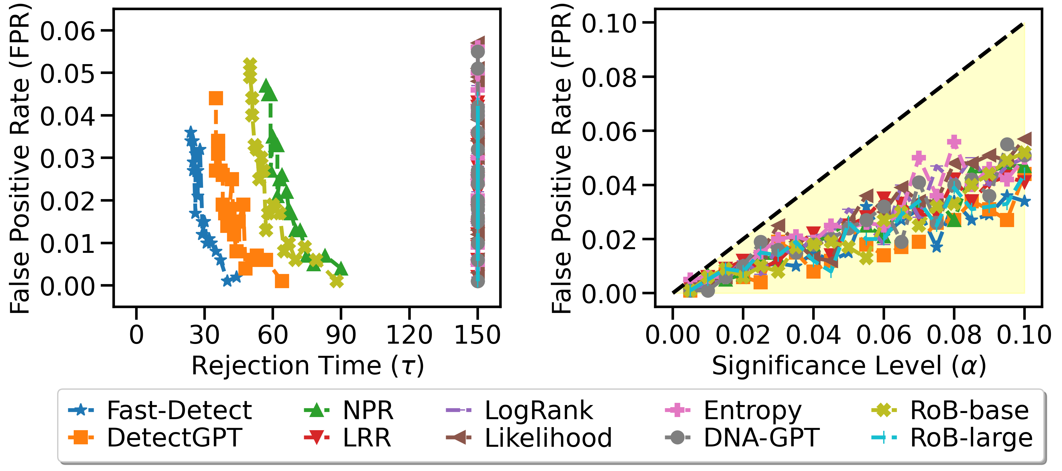
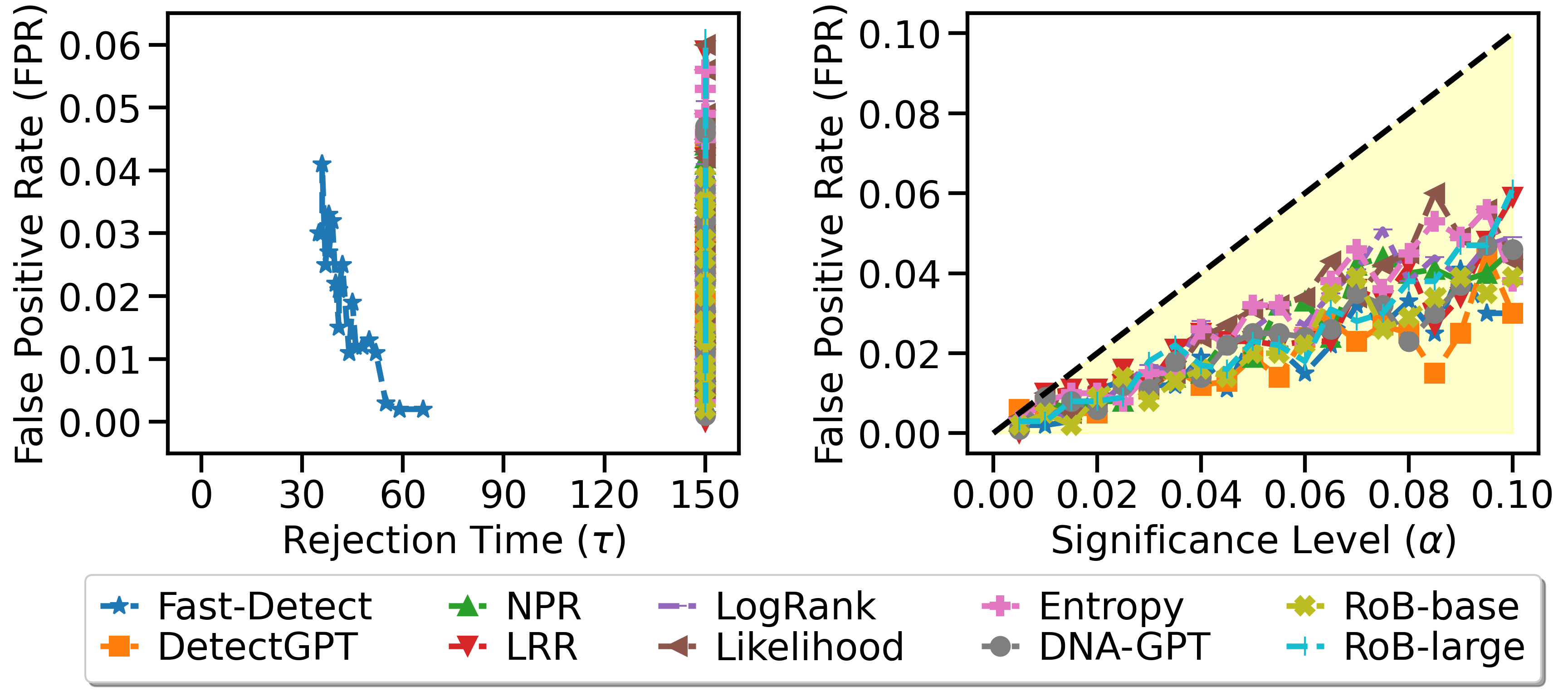

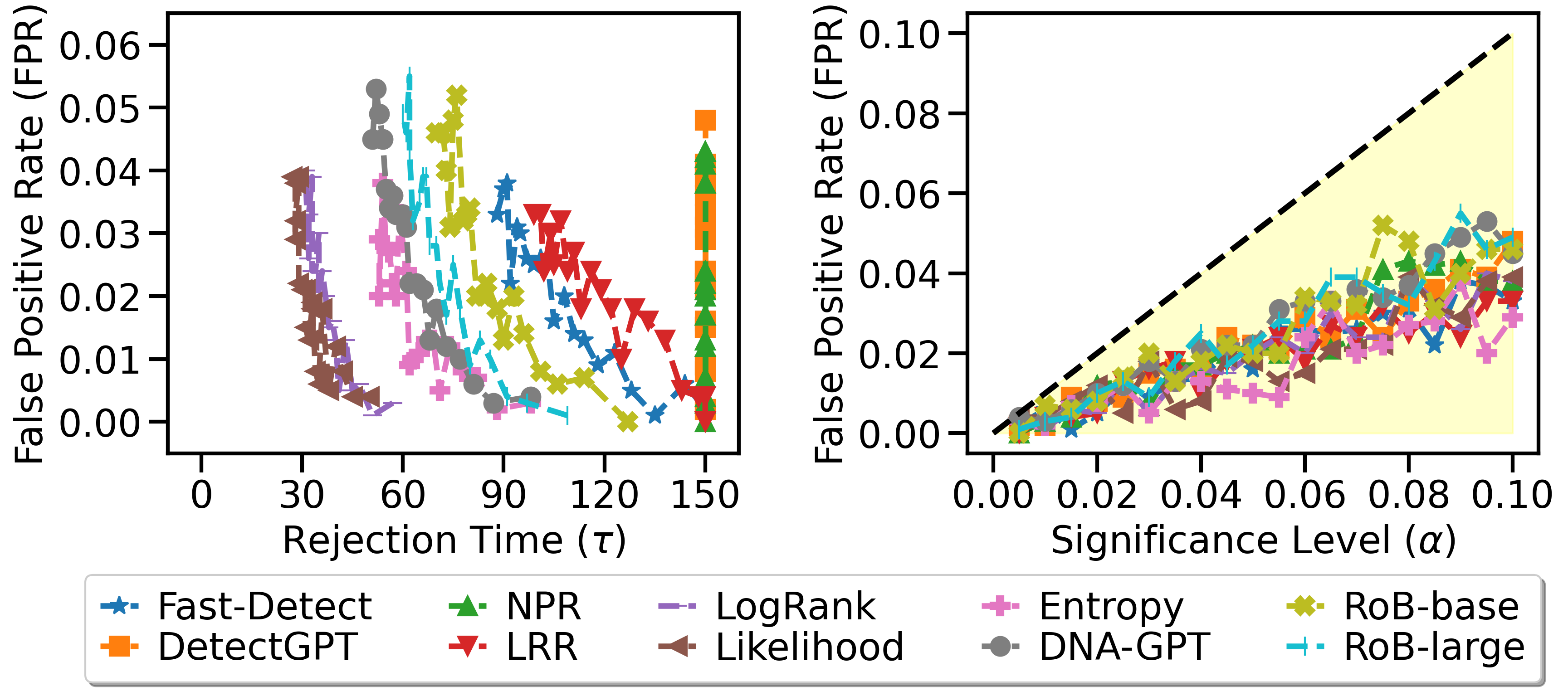
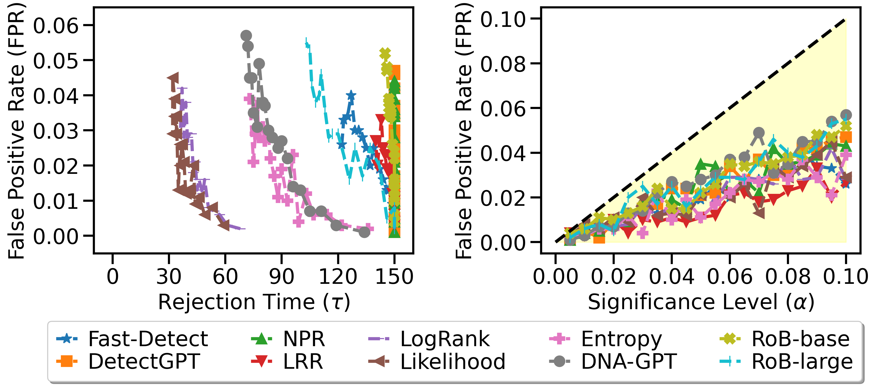
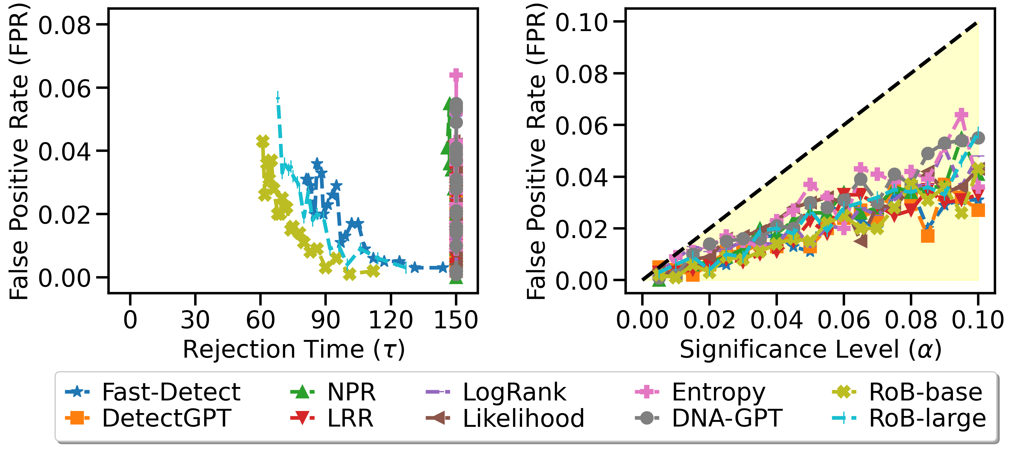
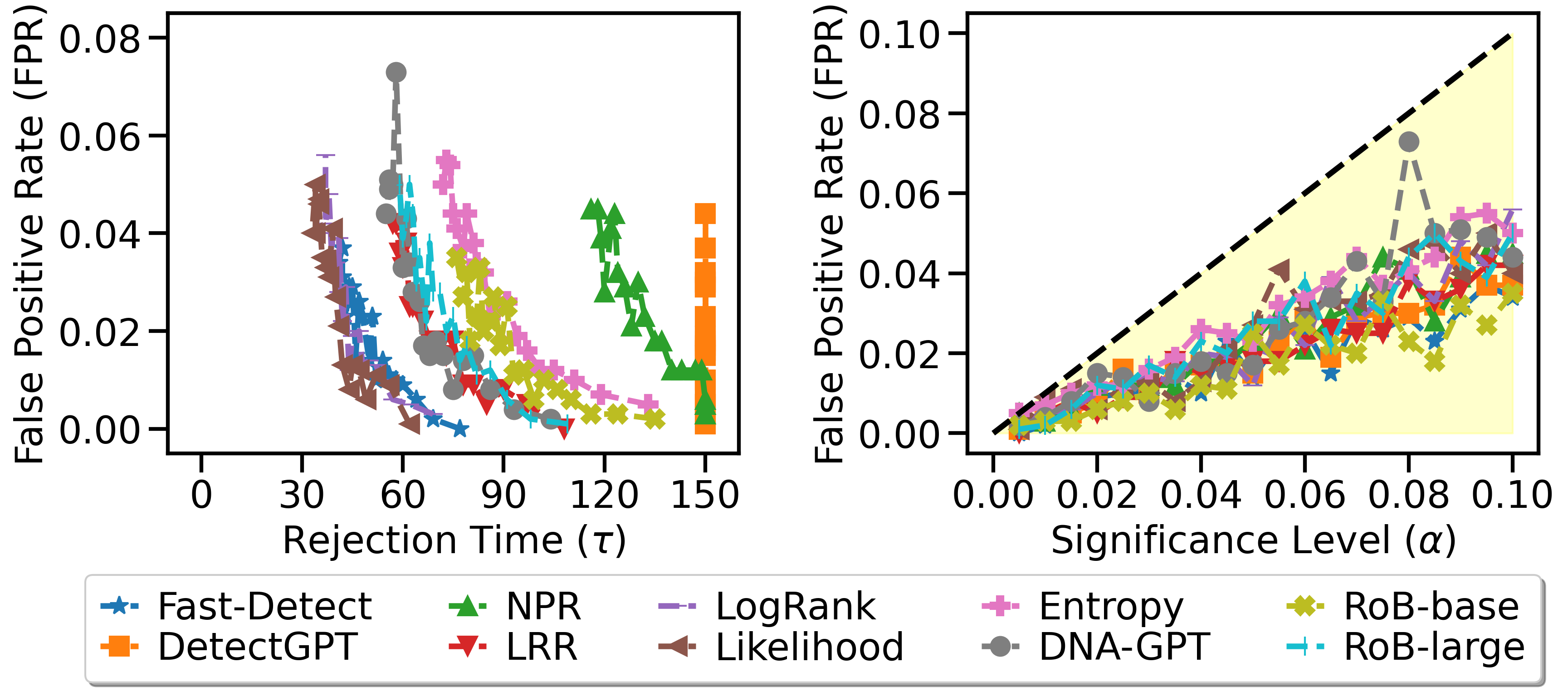
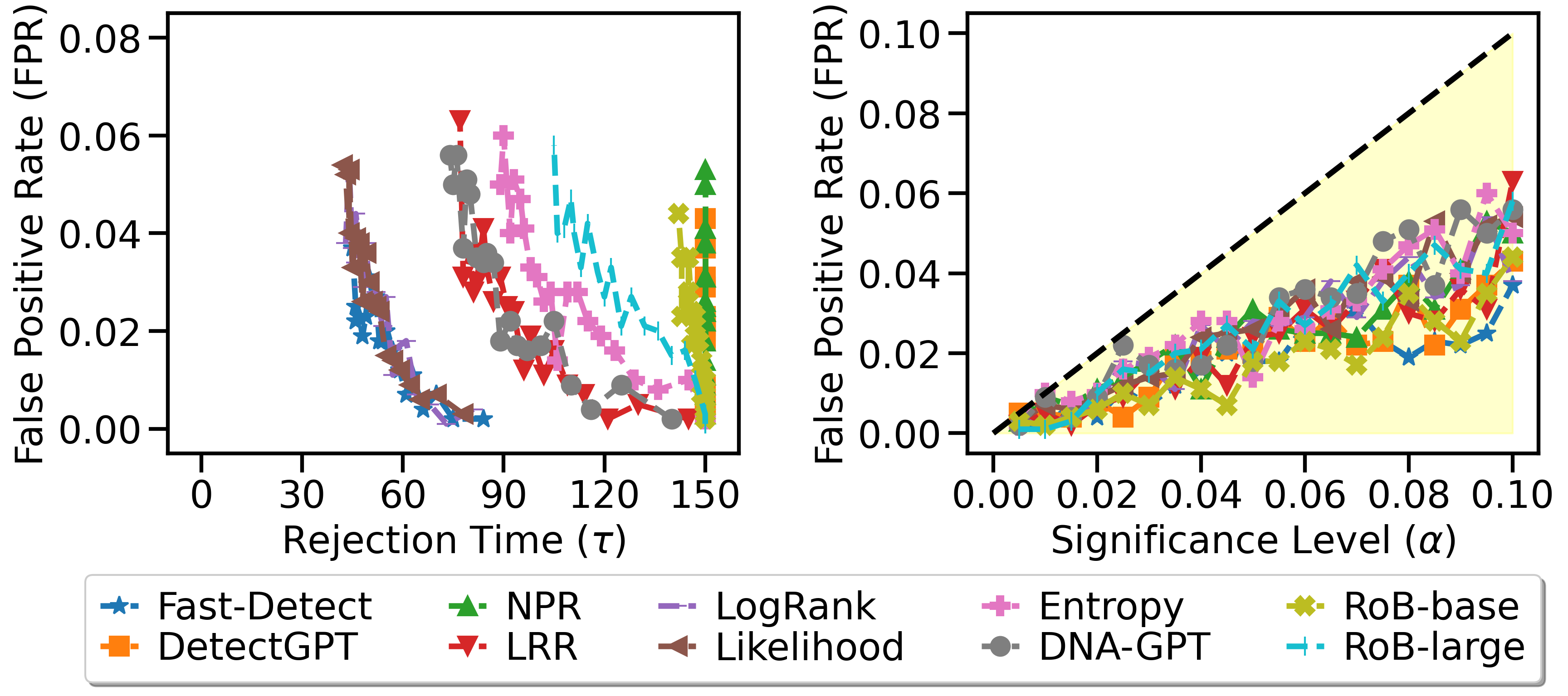
The parameter is chosen from the range . The value of for any is equal to the maximum absolute difference between two sequences of scores for each test, as can be seen in Table 9 for the same-domain texts and Table 9 for the different-domain texts. We get the absolute difference between the scores and for texts from the same domain and different domains involved in our experiments, as shown in the Table 11 and Table 12 respectively. Averaged values of across three source models (GPT-3, ChatGPT and GPT-4) when texts and are from the same domain and different domains are presented in Table 7 and 8, respectively. In practice, we can also select the value of and based on the hint of the bound or by the previous observed samples.
Since we let equal to the actual value of two sequences of human texts, which ensures FPRs of all score functions for each significance level remain below . As we have mentioned previously, our algorithm can ensure a nonnegative supermartingale wealth under and thus control the type-I error. Besides, the relative magnitude of and would influence the rejection time under .
| Scoring Model | Score Function | XSum, XSum | Writing, Writing | PubMed, PubMed | |||
|---|---|---|---|---|---|---|---|
| Human, | Human, | Human, | Human, | Human, | Human, | ||
| LLMs | Human | LLMs | Human | LLMs | Human | ||
| Neo-2.7 | Fast-DetectGPT | 2.2235 | 0.0513 | 2.5690 | 0.0138 | 1.0891 | 0.0179 |
| DetectGPT | 0.4048 | 0.0562 | 0.4985 | 0.0121 | 0.2206 | 0.0061 | |
| NPR | 0.0200 | 0.0025 | 0.0276 | 0.0001 | 0.0135 | 0.0018 | |
| LRR | 0.0919 | 0.0106 | 0.1002 | 0.0047 | 0.0714 | 0.0075 | |
| Logrank | 0.2710 | 0.0303 | 0.4082 | 0.0037 | 0.2707 | 0.0257 | |
| Likelihood | 0.4384 | 0.0420 | 0.6518 | 0.0145 | 0.4604 | 0.0354 | |
| Entropy | 0.1017 | 0.0344 | 0.2393 | 0.0086 | 0.2135 | 0.0243 | |
| DNA-GPT | 0.1917 | 0.0317 | 0.2852 | 0.0232 | 0.5531 | 0.1456 | |
| \hdashline | RoBERTa-base | 0.4585 | 0.0142 | 0.2825 | 0.0186 | 0.1330 | 0.0143 |
| RoBERTa-large | 0.2165 | 0.0090 | 0.1387 | 0.0057 | 0.1088 | 0.0072 | |
| Scoring Model | Score Function | XSum, Writing | XSum, PubMed | Writing, PubMed | |||
|---|---|---|---|---|---|---|---|
| Human, | Human, | Human, | Human, | Human, | Human, | ||
| LLMs | Human | LLMs | Human | LLMs | Human | ||
| Neo-2.7 | Fast-DetectGPT | 2.2848 | 0.2841 | 0.7267 | 0.3624 | 1.0108 | 0.0783 |
| DetectGPT | 0.4828 | 0.0342 | 0.0786 | 0.2992 | 0.0630 | 0.2835 | |
| NPR | 0.0246 | 0.0030 | 0.0115 | 0.0031 | 0.0145 | 0.0012 | |
| LRR | 0.0428 | 0.0665 | 0.0572 | 0.0219 | 0.1094 | 0.0447 | |
| Logrank | 0.1050 | 0.3149 | 0.2429 | 0.0278 | 0.5579 | 0.2872 | |
| Likelihood | 0.1603 | 0.5025 | 0.4548 | 0.0081 | 0.9573 | 0.4969 | |
| Entropy | 0.2071 | 0.4464 | 0.2778 | 0.1154 | 0.7242 | 0.5617 | |
| DNA-GPT | 0.1301 | 0.1551 | 3.0447 | 2.4916 | 3.1997 | 2.6467 | |
| \hdashline | RoBERTa-base | 0.3284 | 0.0459 | 0.3304 | 0.1974 | 0.2844 | 0.1514 |
| RoBERTa-large | 0.1351 | 0.0073 | 0.1962 | 0.0874 | 0.1889 | 0.0801 | |
| Text Domain | Score Functions | Test1 | Test2 | Test3 | |||
|---|---|---|---|---|---|---|---|
| Human, | Human, | Human, | Human, | Human, | Human, | ||
| GPT-3 | Human | ChatGPT | Human | GPT-4 | Human | ||
| XSum, Xsum | Fast-DetectGPT | 7.4812 | 6.0978 | 7.9321 | 5.8211 | 7.1870 | 5.9146 |
| DetectGPT | 2.7997 | 2.3369 | 2.4485 | 2.4753 | 2.0792 | 2.1686 | |
| NPR | 0.2025 | 0.1469 | 0.1418 | 0.1449 | 0.1184 | 0.1248 | |
| LRR | 0.5798 | 0.5798 | 0.6088 | 0.4623 | 0.5913 | 0.5412 | |
| Logrank | 1.3841 | 1.4601 | 1.1775 | 1.0302 | 1.4912 | 1.4399 | |
| Likelihood | 2.1195 | 2.1755 | 1.8610 | 1.5937 | 2.2947 | 2.1624 | |
| Entropy | 2.0369 | 1.9155 | 1.4552 | 1.3976 | 1.9421 | 1.8986 | |
| DNA-GPT | 1.0847 | 0.9399 | 0.9219 | 0.8006 | 1.0386 | 0.9783 | |
| \cdashline2-10 | RoBERTa-base | 0.9997 | 0.9977 | 0.9997 | 0.9977 | 0.9997 | 0.9977 |
| RoBERTa-large | 0.9970 | 0.8191 | 0.9944 | 0.3471 | 0.9862 | 0.8191 | |
| Writing, Writing | Fast-DetectGPT | 8.0598 | 6.5768 | 8.4128 | 5.9812 | 6.6396 | 6.5999 |
| DetectGPT | 3.5032 | 3.1609 | 3.2897 | 3.1502 | 2.7128 | 3.3487 | |
| NPR | 0.2103 | 0.1500 | 0.1920 | 0.1356 | 0.1286 | 0.1502 | |
| LRR | 0.6487 | 0.5483 | 0.7428 | 0.5115 | 0.5417 | 0.4754 | |
| Logrank | 2.1419 | 1.4950 | 1.5963 | 1.4485 | 1.6212 | 1.4024 | |
| Likelihood | 3.3565 | 2.0134 | 2.4280 | 1.8810 | 2.3618 | 2.0046 | |
| Entropy | 2.8300 | 1.6976 | 1.6677 | 1.4732 | 2.0601 | 1.5292 | |
| DNA-GPT | 1.2223 | 1.2879 | 1.1989 | 1.0239 | 1.3639 | 1.2719 | |
| \cdashline2-10 | RoBERTa-base | 0.9997 | 0.9997 | 0.9997 | 0.9997 | 0.9996 | 0.9997 |
| RoBERTa-large | 0.9992 | 0.9172 | 0.9456 | 0.5028 | 0.9172 | 0.9172 | |
| Pubmed, Pubmed | Fast-DetectGPT | 5.6200 | 4.7132 | 5.8150 | 4.8065 | 4.6136 | 4.6400 |
| DetectGPT | 2.0692 | 1.8394 | 2.1635 | 2.3610 | 1.5185 | 2.0677 | |
| NPR | 0.1888 | 0.2020 | 0.1867 | 0.2185 | 0.2028 | 0.2173 | |
| LRR | 0.6811 | 0.7180 | 0.7433 | 0.6000 | 0.8885 | 0.7180 | |
| Logrank | 1.8434 | 2.4121 | 1.9131 | 1.7634 | 2.6000 | 2.3949 | |
| Likelihood | 2.8480 | 3.4780 | 3.1426 | 2.8756 | 3.8419 | 3.5055 | |
| Entropy | 2.0549 | 2.2002 | 2.0570 | 1.8376 | 2.4877 | 2.3156 | |
| DNA-GPT | 5.1276 | 4.7710 | 4.3683 | 4.7319 | 4.9899 | 4.8031 | |
| \cdashline2-10 | RoBERTa-base | 0.9982 | 0.9962 | 0.9984 | 0.9953 | 0.9995 | 0.9963 |
| RoBERTa-large | 0.9688 | 0.8863 | 0.8860 | 0.8863 | 0.8702 | 0.8863 | |
| Text Domain | Score Function | Test1 | Test2 | Test3 | |||
|---|---|---|---|---|---|---|---|
| Human, | Human, | Human, | Human, | Human, | Human, | ||
| GPT-3 | Human | ChatGPT | Human | GPT-4 | Human | ||
| XSum, Writing | Fast-DetectGPT | 7.7260 | 6.2430 | 8.0558 | 6.0578 | 7.3268 | 6.1780 |
| DetectGPT | 3.1711 | 2.8288 | 2.8371 | 2.6976 | 2.5561 | 2.6884 | |
| NPR | 0.2001 | 0.1398 | 0.1736 | 0.1571 | 0.1249 | 0.1352 | |
| LRR | 0.5817 | 0.5355 | 0.6395 | 0.6469 | 0.4837 | 0.5354 | |
| Logrank | 1.8576 | 1.6371 | 1.4423 | 1.7444 | 1.0620 | 1.5484 | |
| Likelihood | 3.1515 | 2.2793 | 2.0097 | 2.3806 | 1.5890 | 2.3587 | |
| Entropy | 2.6910 | 2.0533 | 1.8358 | 2.0545 | 1.5863 | 1.7798 | |
| DNA-GPT | 1.0351 | 1.3620 | 0.8960 | 1.1271 | 0.7700 | 1.1035 | |
| \cdashline2-10 | RoBERTa-base | 0.9997 | 0.9920 | 0.9997 | 0.9997 | 0.9996 | 0.9997 |
| RoBERTa-large | 0.9992 | 0.9172 | 0.9455 | 0.3471 | 0.2952 | 0.5028 | |
| XSum, Pubmed | Fast-DetectGPT | 5.7796 | 5.2418 | 6.0477 | 5.5643 | 5.2864 | 5.5884 |
| DetectGPT | 1.9280 | 2.1249 | 2.2991 | 2.7521 | 2.0123 | 2.8121 | |
| NPR | 0.1529 | 0.1813 | 0.1607 | 0.1745 | 0.1608 | 0.1609 | |
| LRR | 0.7144 | 0.6422 | 0.6765 | 0.5376 | 0.6952 | 0.5247 | |
| Logrank | 1.6718 | 2.2405 | 1.3408 | 1.6702 | 1.3285 | 1.5756 | |
| Likelihood | 2.4632 | 3.1031 | 2.3094 | 2.5604 | 2.2453 | 2.3964 | |
| Entropy | 2.2528 | 2.3452 | 1.9397 | 1.6543 | 1.9994 | 1.8273 | |
| DNA-GPT | 6.6172 | 6.2606 | 5.6482 | 6.0117 | 6.3382 | 6.0307 | |
| \cdashline2-10 | RoBERTa-base | 0.9983 | 0.9964 | 0.9984 | 0.9976 | 0.9995 | 0.9976 |
| RoBERTa-large | 0.9688 | 0.8191 | 0.8610 | 0.8863 | 0.8703 | 0.8863 | |
| Writing, Pubmed | Fast-DetectGPT | 4.9091 | 5.3870 | 6.3816 | 5.4647 | 5.8265 | 5.3231 |
| DetectGPT | 2.7326 | 2.9296 | 2.5926 | 3.0456 | 2.3285 | 3.1283 | |
| NPR | 0.1546 | 0.1829 | 0.1609 | 0.1927 | 0.1733 | 0.1588 | |
| LRR | 0.7289 | 0.6567 | 0.8526 | 0.7093 | 0.8070 | 0.6364 | |
| Logrank | 1.7772 | 2.0524 | 2.0617 | 1.8547 | 1.8669 | 1.6617 | |
| Likelihood | 2.6541 | 2.8230 | 3.1136 | 2.6684 | 3.0234 | 2.6871 | |
| Entropy | 2.4478 | 2.5402 | 2.6542 | 2.3688 | 2.3984 | 2.2263 | |
| DNA-GPT | 7.0524 | 6.6958 | 6.0130 | 6.3766 | 6.6221 | 6.3146 | |
| \cdashline2-10 | RoBERTa-base | 0.9983 | 0.9964 | 0.9996 | 0.9995 | 0.9996 | 0.9996 |
| RoBERTa-large | 0.9688 | 0.9172 | 0.8610 | 0.8863 | 0.8703 | 0.8863 | |
| Text Domain | Score Function | Test1 | Test2 | Test3 | |||
|---|---|---|---|---|---|---|---|
| Human, | Human, | Human, | Human, | Human, | Human, | ||
| GPT-3 | Human | ChatGPT | Human | GPT-4 | Human | ||
| XSum, Xsum | Fast-DetectGPT | 1.9598 | 0.0770 | 2.9471 | 0.0106 | 1.7638 | 0.0664 |
| DetectGPT | 0.5656 | 0.0729 | 0.4816 | 0.0114 | 0.1672 | 0.0844 | |
| NPR | 0.0305 | 0.0031 | 0.0248 | 0.0006 | 0.0047 | 0.0037 | |
| LRR | 0.0349 | 0.0159 | 0.1568 | 0.0032 | 0.0839 | 0.0127 | |
| Logrank | 0.1938 | 0.0455 | 0.3794 | 0.0077 | 0.2397 | 0.0378 | |
| Likelihood | 0.3488 | 0.0630 | 0.5960 | 0.0109 | 0.3704 | 0.0521 | |
| Entropy | 0.0586 | 0.0517 | 0.1456 | 0.0117 | 0.1009 | 0.0400 | |
| DNA-GPT | 0.1579 | 0.0476 | 0.2742 | 0.0287 | 0.1432 | 0.0188 | |
| \cdashline2-8 | RoBERTa-base | 0.5939 | 0.0210 | 0.5946 | 0.0002 | 0.1871 | 0.0212 |
| RoBERTa-large | 0.3941 | 0.0133 | 0.2037 | 0.0001 | 0.0516 | 0.0135 | |
| Writing, Writing | Fast-DetectGPT | 2.3432 | 0.0204 | 3.1805 | 0.0206 | 2.1831 | 0.0002 |
| DetectGPT | 0.5752 | 0.0181 | 0.6980 | 0.0093 | 0.2223 | 0.0088 | |
| NPR | 0.0330 | 0.0001 | 0.0415 | 0.0001 | 0.0083 | 0.0001 | |
| LRR | 0.0979 | 0.0062 | 0.1512 | 0.0009 | 0.0516 | 0.0070 | |
| Logrank | 0.3737 | 0.0055 | 0.5407 | 0.0026 | 0.3103 | 0.0028 | |
| Likelihood | 0.5915 | 0.0217 | 0.8511 | 0.0046 | 0.5126 | 0.0171 | |
| Entropy | 0.2260 | 0.0130 | 0.3428 | 0.0036 | 0.1490 | 0.0093 | |
| DNA-GPT | 0.2441 | 0.0348 | 0.3745 | 0.0155 | 0.2370 | 0.0193 | |
| \cdashline2-8 | RoBERTa-base | 0.6070 | 0.0279 | 0.2184 | 0.0093 | 0.0220 | 0.0186 |
| RoBERTa-large | 0.3845 | 0.0085 | 0.0143 | 0.0033 | 0.0175 | 0.0052 | |
| Pubmed, Pubmed | Fast-DetectGPT | 0.7397 | 0.0025 | 1.3683 | 0.0243 | 1.1594 | 0.0268 |
| DetectGPT | 0.2417 | 0.0092 | 0.2470 | 0.0051 | 0.1729 | 0.0041 | |
| NPR | 0.0146 | 0.0015 | 0.0175 | 0.0012 | 0.0084 | 0.0028 | |
| LRR | 0.0101 | 0.0070 | 0.1099 | 0.0042 | 0.0944 | 0.0112 | |
| Logrank | 0.0282 | 0.0293 | 0.4115 | 0.0092 | 0.3725 | 0.0385 | |
| Likelihood | 0.0771 | 0.0411 | 0.6922 | 0.0121 | 0.6119 | 0.0532 | |
| Entropy | 0.0766 | 0.0316 | 0.2939 | 0.0048 | 0.2701 | 0.0364 | |
| DNA-GPT | 0.3518 | 0.1309 | 0.8721 | 0.0875 | 0.4354 | 0.2184 | |
| \cdashline2-8 | RoBERTa-base | 0.1859 | 0.0078 | 0.1666 | 0.0137 | 0.0466 | 0.0215 |
| RoBERTa-large | 0.1318 | 0.0077 | 0.1294 | 0.0031 | 0.0652 | 0.0108 | |
| Text Domain | Score Functions | Test1 | Test2 | Test3 | |||
|---|---|---|---|---|---|---|---|
| Human, | Human, | Human, | Human, | Human, | Human, | ||
| GPT-3 | Human | ChatGPT | Human | GPT-4 | Human | ||
| XSum, Writing | Fast-DetectGPT | 2.1206 | 0.2430 | 2.8602 | 0.2996 | 1.8737 | 0.3096 |
| DetectGPT | 0.6211 | 0.0278 | 0.6617 | 0.027 | 0.1657 | 0.0478 | |
| NPR | 0.0323 | 0.0008 | 0.0377 | 0.0038 | 0.0039 | 0.0044 | |
| LRR | 0.0391 | 0.0526 | 0.0757 | 0.0747 | 0.0137 | 0.0723 | |
| Logrank | 0.0893 | 0.2899 | 0.2081 | 0.33 | 0.0175 | 0.3249 | |
| Likelihood | 0.1362 | 0.4771 | 0.3281 | 0.5184 | 0.0166 | 0.5121 | |
| Entropy | 0.1843 | 0.4233 | 0.1228 | 0.462 | 0.3142 | 0.4539 | |
| DNA-GPT | 0.1279 | 0.1509 | 0.1953 | 0.1638 | 0.0672 | 0.1505 | |
| \cdashline2-8 | RoBERTa-base | 0.6513 | 0.0163 | 0.2744 | 0.0653 | 0.0596 | 0.0562 |
| RoBERTa-large | 0.3789 | 0.0029 | 0.0253 | 0.0078 | 0.0011 | 0.0112 | |
| XSum, Pubmed | Fast-DetectGPT | 0.4179 | 0.3244 | 0.9937 | 0.3989 | 0.7686 | 0.3639 |
| DetectGPT | 0.0098 | 0.2424 | 0.0723 | 0.3245 | 0.1538 | 0.3308 | |
| NPR | 0.0148 | 0.0017 | 0.0133 | 0.0029 | 0.0064 | 0.0048 | |
| LRR | 0.0214 | 0.0184 | 0.0868 | 0.0273 | 0.0633 | 0.0199 | |
| Logrank | 0.0349 | 0.0226 | 0.3819 | 0.0388 | 0.312 | 0.0219 | |
| Likelihood | 0.1195 | 0.0014 | 0.6838 | 0.0205 | 0.5612 | 0.0024 | |
| Entropy | 0.0782 | 0.1232 | 0.4019 | 0.1032 | 0.3533 | 0.1197 | |
| DNA-GPT | 2.8511 | 2.6302 | 3.2363 | 2.4517 | 3.0468 | 2.3930 | |
| \cdashline2-8 | RoBERTa-base | 0.3711 | 0.193 | 0.3591 | 0.2063 | 0.2609 | 0.1928 |
| RoBERTa-large | 0.2087 | 0.0846 | 0.2165 | 0.0902 | 0.1633 | 0.0873 | |
| Writing, Pubmed | Fast-DetectGPT | 0.6609 | 0.0813 | 1.2933 | 0.0993 | 1.0782 | 0.0543 |
| DetectGPT | 0.0376 | 0.2702 | 0.0453 | 0.2974 | 0.1060 | 0.2830 | |
| NPR | 0.0156 | 0.0025 | 0.0170 | 0.0008 | 0.0108 | 0.0004 | |
| LRR | 0.0312 | 0.0342 | 0.1614 | 0.0474 | 0.1356 | 0.0525 | |
| Logrank | 0.3248 | 0.2673 | 0.7119 | 0.2912 | 0.6369 | 0.3030 | |
| Likelihood | 0.5966 | 0.4785 | 1.2021 | 0.4978 | 1.0733 | 0.5145 | |
| Entropy | 0.5015 | 0.5465 | 0.8638 | 0.5651 | 0.8072 | 0.5735 | |
| DNA-GPT | 3.002 | 2.7812 | 3.4000 | 2.6155 | 3.1972 | 2.5435 | |
| \cdashline2-8 | RoBERTa-base | 0.3548 | 0.1767 | 0.2939 | 0.1410 | 0.2046 | 0.1366 |
| RoBERTa-large | 0.2057 | 0.0817 | 0.2088 | 0.0825 | 0.1521 | 0.0761 | |