Foreground signals minimally affect inference of high-mass binary black holes in next generation gravitational-wave detectors

Abstract

Next-generation gravitational-wave observatories are expected to detect over a thousand compact binary coalescence signals daily, with some lasting from minutes to hours. Consequently, multiple signals will overlap in the time-frequency plane, generating a ”foreground noise” that predominantly affects the low-frequency range, where binary neutron star inspiral evolution is gradual. This study investigates the impact of such foreground noise on parameter estimation for short-duration binary black hole signals, particularly those with high detector-frame masses and/or located at large redshifts. Our results show a reduction in detection sensitivity by approximately 25% when the noise power spectrum deviates by up to 50% from Gaussian noise due to foreground contamination. Despite this, using standard parameter estimation techniques without subtracting overlapping signals, we find that foreground noise has minimal impact, primarily affecting precision. These findings suggest that even in the presence of substantial foreground noise, global-fit techniques, and/or signal subtraction will not be necessary, as accurate recovery of system parameters is achievable with minimal loss in precision.

I Introduction

The next-generation (XG) of terrestrial gravitational-wave (GW) observatories, such as the Einstein Telescope (ET) [1, 2, 3] and Cosmic Explorer (CE) [4, 5, 6], are anticipated to begin operations in the mid-2030s. These observatories will offer an order-of-magnitude improvement in sensitivity over current GW detectors, with a broader frequency bandwidth that enhances detection capabilities at both low and high frequencies (see Fig. 1). Consequently, the detection rate of compact binary coalescences will increase significantly, with observable signals lasting from minutes to hours [7, 8, 9, 10, 11].

This dramatic improvement will lead to overlapping signals in the detectors’ output. The number of overlapping signals depends on both the astrophysical merger rate density and the detectors’ extended reach (see Appendix A for an estimate). These signals, particularly those at low frequencies where the inspiral evolution is gradual, will overlap in the time-frequency plane, gradually separating as they approach the merger phase. Current matched-filter searches can uniquely identify such events and determine their merger times with millisecond accuracy [12]. Thus, unlike the source confusion expected in LISA, where overlapping white dwarf binary signals may not be uniquely identified [13], overlapping signals in ground-based XG detectors are resolvable and primarily contribute as foreground noise [14, 15, 16].

This foreground noise arises from both detectable and undetectable signals, with the latter typically having a single-detector signal-to-noise ratio (SNR) of $\lesssim 5$. Although detectable signals can be subtracted from the data, achieving perfect subtraction remains challenging. Significant residuals may persist due to waveform systematics, as demonstrated by Antonelli et al. [17], potentially introducing biases. Moreover, the subtraction process is subject to both statistical and systematic uncertainties, further complicating the analysis.

In addition, Reali et al. [18] noted that the collection of undetectable signals can affect parameter estimation (PE), broadening the posterior distributions by distorting the noise power spectral density (PSD) estimates. This arises because the small number of overlapping signals per time-frequency bin does not conform to the central limit theorem, preventing the foreground noise from being modelled as Gaussian. Furthermore, as these signals evolve, the data can no longer be considered wide-sense stationary, violating the assumptions of current noise PSD estimation methods such as Welch averaging [19] and BayesLine [20]. As a result, inaccurate PSD estimates can degrade the efficacy of GW searches and parametric inference. Pizzati et al. [21] and Samajdar et al. [22] further showed that overlapping signals with comparable SNRs observed within a short time interval ($\sim\mathcal{O}(1\,\mathrm{s})$) can bias posterior estimates, depending on the nature of the source.

In this paper, we investigate the impact of foreground noise on Bayesian posterior estimates when detected signals are not subtracted from the data. Since overlaps predominantly occur at low frequencies, foreground noise primarily affects low-frequency PSD estimates (see Fig. 2). This is particularly important for high detector-frame mass systems, such as intermediate-mass black hole (IMBH) binaries or stellar-mass binary black holes at large redshifts [23, 24, 25], as these systems may merge at frequencies below 20 Hz. Therefore, we restrict our focus to these sources.

Prior to the fourth observing run of Advanced LIGO [26] and Virgo [27], only a few events with a total detector-frame mass exceeding $100M_{\odot}$ have been detected [28, 29, 30]. However, XG observatories are expected to detect $\mathcal{O}(1000)$ IMBH binaries annually, contingent on population assumptions. A subset of these events will be detected with SNR values on the order of $\mathcal{O}(100)$, allowing source-frame mass constraints with errors as low as $\lesssim 1\%$ [8, 31].

Binaries originating from Population-III stars are also expected to be detected by XG detectors. Current population synthesis studies suggest that the merger rate of these BBHs may peak at redshift $z\sim 15$, reaching merger rates of $\mathcal{O}(10^{-1}-10^{2})/\mathrm{Gpc}^{3}/\mathrm{yr}$ [32, 33, 25, 34, 35, 36]. A confident detection of a BBH merger at such high redshifts could provide strong evidence of their Population III origins. With total detector-frame masses below $1500M_{\odot}$, these systems will merge within the frequency range of XG detectors. Gupta et al. [8] showed that a network of XG detectors will not only detect most Population III BBH mergers but will also constrain their source-frame masses and redshifts to within $\mathcal{O}(10\%)$ precision.

While all these studies have provided valuable insights, they either neglected foreground noise effects or employed Fisher matrix analyses. Consequently, their parameter precision estimates may not fully capture the limitations of XG detectors. This work addresses these gaps by incorporating more realistic data simulations and Bayesian inference techniques. This allows us to more accurately assess the true potential of XG observatories in detecting and characterizing intermediate-mass and Population III BBHs.

Our analysis reveals a reduction in detection sensitivity of $\sim 25\%$ when the noise power spectrum deviates by approximately 50% from Gaussian noise levels due to foreground noise. While foreground noise degrades the inferred parameters’ precision, potentially limiting the full scientific capability of XG detectors, it does not introduce significant biases. Importantly, the true parameter values consistently remain within the 90% credible intervals. These results indicate that even in scenarios with significant foreground noise, the need for global-fit techniques or signal subtraction may be unnecessary, as the recovery of system parameters remains accurate with only a minimal loss in precision.

The remainder of this paper is organized as follows. In Section II, we provide an overview of the detector network, detail the likelihood function, and describe the methodology for modelling foreground noise in our analysis. Section III outlines the analysis setup and procedures used to generate the results presented in Section IV. Finally, Section V presents our conclusions and discusses potential directions for future research.

II Detector network, likelihood and foreground noise

The interplay between foreground noise and detector sensitivity is crucial for understanding how overlapping gravitational wave signals can influence binary parameter inference. This section outlines the detector network used in our analysis, the likelihood function employed for signal inference, and the approach to modelling foreground noise.

II.1 Detector network

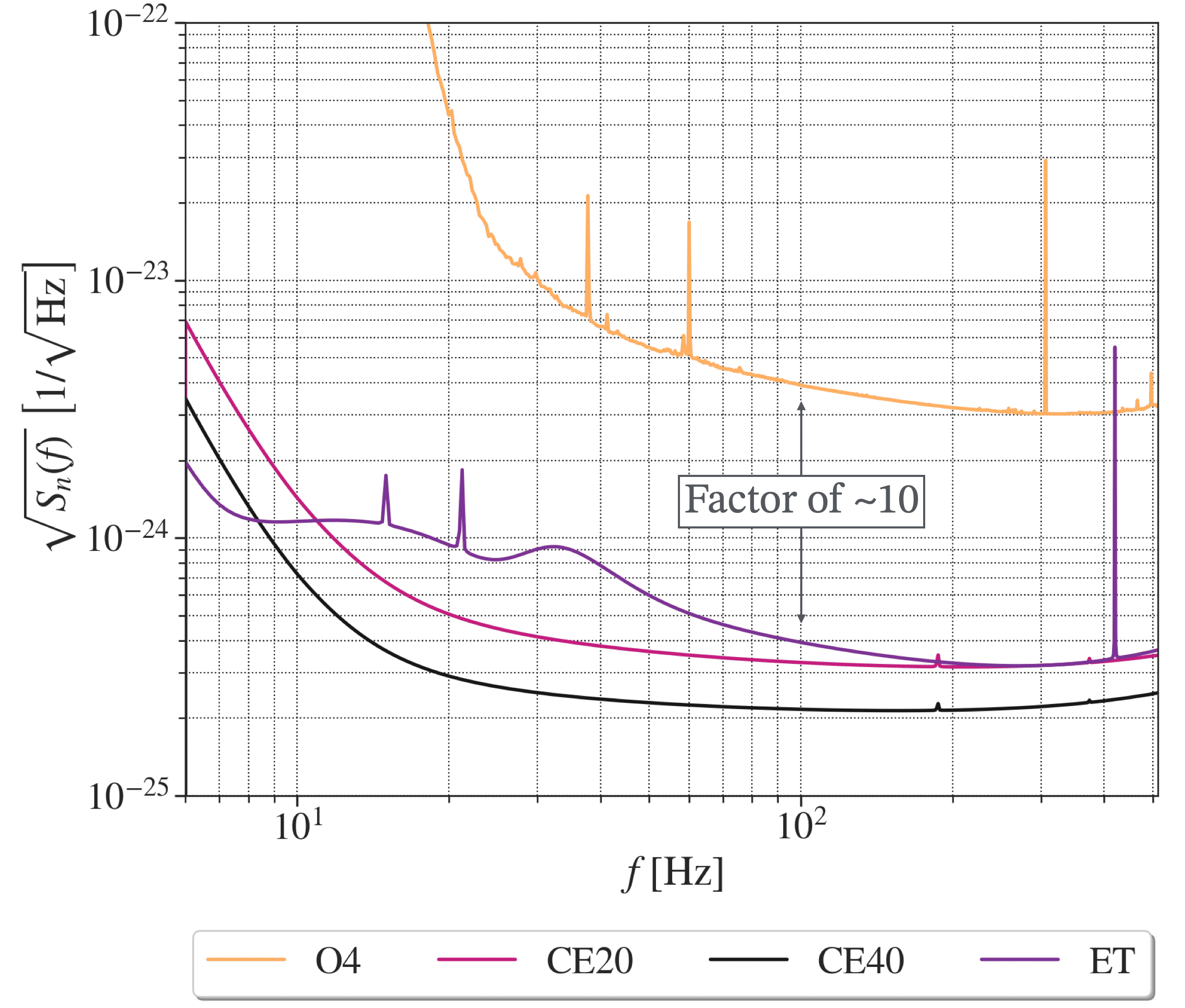
Figure 1: Amplitude spectral densities $\sqrt{S_{n}(f)}$ of the Advanced LIGO Livingston detector (in O4 run) and XG gravitational-wave detectors. The $\sqrt{S_{n}(f)}$ for Advanced LIGO Livingston is estimated using data surrounding the event GW230529 [37, 38]. The XG detectors are expected to achieve sensitivities at least an order of magnitude greater than current detectors, significantly improving the detection capability across a wider frequency range.

We consider a three-detector network composed of a 40 km and a 20 km L-shaped CE observatory (henceforth CE40 and CE20), along with a triangle-shaped ET featuring 10 km arms, as implemented in gwforge [16]. Since the exact locations of these detector sites are yet to be finalized, following Vitale et al. [39], we place the CE detectors at two sites separated by a distance comparable to the size of the continental US. For ET, we adopt the potential site in Sardinia. The design noise curves for all these detectors are shown in Fig. 1, providing a schematic understanding of how much more sensitive they will be as compared to the Advanced LIGO-Livingston detector in its fourth observing run.

II.2 Detector data and the likelihood function

The time-varying output of current GW detectors is modelled as the sum of two additive components: the detector noise $\bm{n}$ and the target signal $\bm{s}_{T}(\bm{\theta})$. For quasi-spherical BBH signals, the parameter vector $\bm{\theta}$ is 15-dimensional and includes the component masses $m_{i}$, and their spins $\bm{\chi}_{i}$, the luminosity distance $D_{L}$, the sky-location parameters $(\alpha,\delta)$, the binary orientation parameters $(\iota,\phi)$, the polarization angle $\psi$, and the merger time $t_{c}$.

The noise $\bm{n}$ is typically assumed to follow a zero-mean, wide-sense stationary, Gaussian process. Under these assumptions, the noise properties are completely characterised by the noise covariance matrix:

$$\langle|\tilde{n}_{k}|^{2}\rangle=\frac{T}{2}S_{n}(f_{k})~{}.$$ (1)

Here $\tilde{n}_{k}$ is the complex amplitude of the discrete Fourier transform of $\bm{n}$ at frequency $f_{k}$, $T$ is the analysis duration, and $S_{n}(f_{k})$ is the noise PSD.

The objective of modelled signal analysis is to find a template signal $\bm{h}(\bm{\theta}^{\prime})$ that accurately represents the target signal $\bm{s}_{T}(\bm{\theta})$, such that the residual $\bm{d}-\bm{h}$ conforms to the noise distribution. This means that the noise model defines the likelihood function. Therefore, for CBC analysis, we consider the following likelihood function:

$$\mathfrak{L}\left(\bm{d}\mid S_{n},\bm{\theta}\right)\propto\exp\left[-\sum_{k}\frac{2\left|\tilde{d}_{k}-\tilde{h}_{k}(\bm{\theta}^{\prime})\right|^{2}}{TS_{n}(f_{k})}\right].$$ (2)

When analysing a multi-detector signal, we use the joint likelihood, which is the product of individual detector likelihoods, while ensuring that the signal is coherent across the network. This follows from our assumption that non co-located detectors have independent noise properties. Bayesian PE routines, such as Bilby [40], aim to estimate the signal parameters by solving:

$$p(\bm{\theta}\mid d)\propto\mathcal{L}(d\mid\bm{\theta})\pi(\bm{\theta}),$$ (3)

for each parameter vector $\bm{\theta}$ drawn from the joint prior distribution $\pi(\bm{\theta})$. Thus, the precision of the posterior estimates $p(\bm{\theta}\mid d)$ is directly influenced by the accuracy of the noise power spectrum $S_{n}(f)$.

In XG detectors, multiple signals will be present at a given instance. As a result, the detector data should be assumed as follows:

$$\bm{d}=\bm{n}+\sum_{k\neq T}\bm{s}_{k}(\bm{\theta}_{k})+\bm{s}_{T}(\bm{\theta})~{}.$$ (4)

where $\sum_{k\neq T}\bm{s}_{k}(\bm{\theta}_{k})$ is the collection of all other signals. This will complicate binary PE in two ways. First, the residual $\bm{d}-\bm{h}$ is no longer wide-sense stationary as it contains several rapidly-evolving signals. Therefore, it will be incorrect to use Eq. (2). Second, even when estimating the PSD “off-source”, meaning computing the PSD using data segments that exclude the analysis segment that contains $\bm{s}_{T}(\bm{\theta})$, we will still not be measuring the detector’s noise properties but will measure the combined effect of the detector noise and the contribution coming from the foreground noise. In other words, we won’t be measuring $S_{n}(f)$ but rather $S_{-s_{T}}(f)=S_{n+\sum_{k\neq T}\bm{s}_{k}}(f)$.

It is possible to overcome both of these problems by jointly inferring the noise power spectrum and $\bm{\Theta}=\{\bm{\theta}_{k}\}$, which is the concatenation of all the binary parameters of all the signals in the analysis segment. However, this is currently computationally prohibitive. Hence, we resort to estimating $S_{-s_{T}}(f)$ and gauge the affect of this choice on PE of short-duration signals.

II.3 Foreground Noise

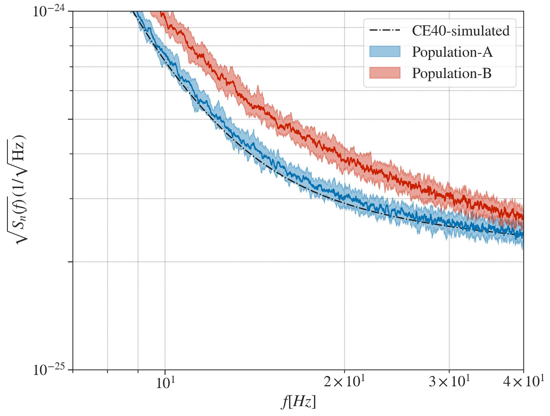
Figure 2: Comparison of Welch estimates for different realizations of 512 seconds of CE40 mock data. The black dotted line represents the design CE40 sensitivity curve. The red curve indicates the estimate when the noise includes signals from Population A, while the blue curve represents the estimate when the noise includes signals from Population B. Both the red and blue curves include a 90% confidence band. The comparison demonstrates that depending on the number of signals, the $\sqrt{S_{n}(f)}$ estimate can deviate from the expected at lower frequencies.

To demonstrate the impact of foreground noise on PSD estimates, we use gwforge to simulate multiple realizations of 8192-seconds long mock XG detector data [16] . The binary parameter distributions used in the simulations are described in detail in Chandra [41]. We consider two distinct sets of merger rate densities: Population A, with a BNS merger rate of $\mathcal{R}_{\textrm{BNS}}=320/\mathrm{Gpc}^{3}/\mathrm{yr}$, black hole neutron star (BHNS) merger rate of $\mathcal{R}_{\textrm{BHNS}}=45/\mathrm{Gpc}^{3}/\mathrm{yr}$, and BBH merger rate of $\mathcal{R}_{\textrm{BBH}}=22/\mathrm{Gpc}^{3}/\mathrm{yr}$, and Population B, with $\mathcal{R}_{\textrm{BNS}}=1700/\mathrm{Gpc}^{3}/\mathrm{yr}$, $\mathcal{R}_{\textrm{BHNS}}=140/\mathrm{Gpc}^{3}/\mathrm{yr}$, and $\mathcal{R}_{\textrm{BBH}}=44/\mathrm{Gpc}^{3}/\mathrm{yr}$. The local merger rates in Population A correspond to the median merger rates inferred using data from the third observing run of Advanced LIGO and Advanced Virgo, whereas the ones in Population B correspond to the upper limit of the inferred rates [42]. The binaries were distributed in redshift following the Madau-Dickinson star-formation rate [43].

The BNS signals were generated using the quasi-circular BNS waveform model IMRPhenomPv2_NRTidalv2 [44], while the BHNS and BBH signals were modelled using the quasi-spherical BBH approximant IMRPhenomXPHM [45]. These signals are then added to 8192-second-long realisations of Gaussian noise, coloured by the XG detector noise power spectra. This resulted in two distinct datasets: one corresponding to Population A and the other to Population B.

To evaluate the effect of these foreground signals on PSD estimates, we employed the median-mean Welch method to estimate $S_{-\bm{s}_{T}}(f)$ across multiple realizations of both datasets. The Welch method assumes that the data is wide-sense stationary, dividing the discrete time-domain data $d[j]$ into $K$ overlapping segments $d_{k}[j]$ of length $L$, each windowed by $w[j]$— in this case, a Hann window function. The discrete Fourier transform $\widetilde{d}_{k}[i]$ of each windowed segment is computed using an FFT routine, and the periodogram $P_{k}[i]$ is obtained as follows:

$$P_{k}[i]=\frac{1}{U}\left|d_{k}[i]\right|^{2},$$ (5)

where $U=\sum_{n=0}^{L-1}w[j]^{2}$. Following Allen et al. [19], we then apply mean-median averaging to the periodograms across all segments to obtain the final PSD estimate, as this method significantly reduces the variance of the spectral estimate due to non-stationarity.

Fig. 2 displays the simulated and estimated CE40 $\sqrt{S_{-\bm{s}_{T}}(f)}$, with the latter derived using the Welch method. The estimation was performed by dividing each 512-second realisation of data into 16-second subsegments with 50% overlap, similar to the approach used in a PyCBC search [46]. Consistent with previous studies [14, 16], we observed that the deviation is primarily concentrated at frequencies lower than 30 Hz, reaching values of $\gtrsim 50\%$ at 15 Hz for the higher merger rate density and CE40 detector. This can reduce the detectability of BBHs with a high detector frame (redshifted) total mass, as shown in Fig. 3. In particular, depending on the binary’s detector frame mass, the horizon distance  loss to systems with $M_{T}(1+z)\gtrsim 1000M_{\odot}$ can be $\gtrsim 30\%$.

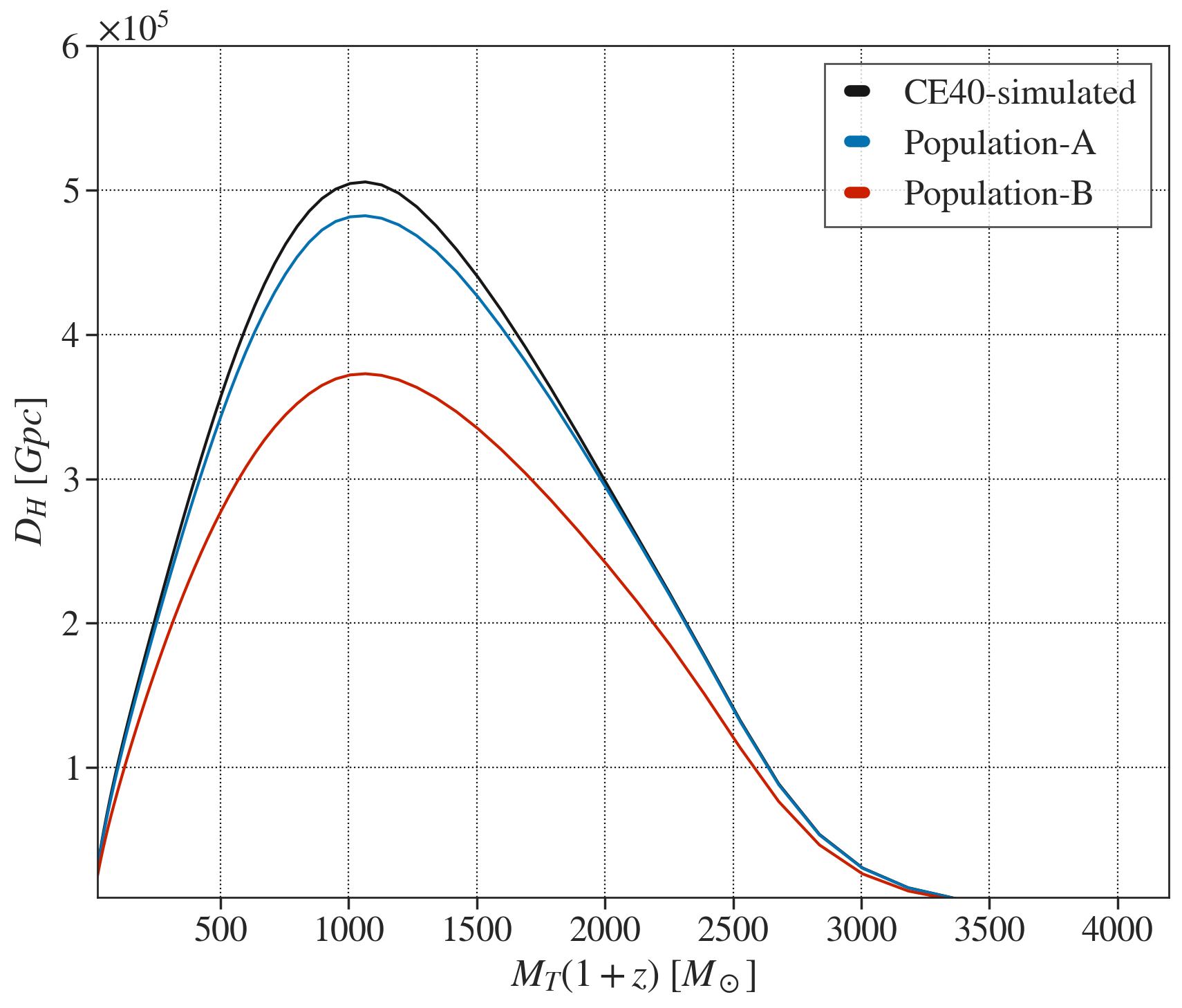
Figure 3: Comparison of horizon distance reach when using the median Welch ASD estimates. The black dotted line represents the ideal CE40 design sensitivity curve. The red curve indicates the estimate when the noise includes signals from population A, while the blue curve represents the estimate when the noise includes signals from population B. The comparison shows that depending on the number of signals, the horizon distance of a XG detector can be affected, especially for BBHs with a high detector frame (redshifted) total mass.

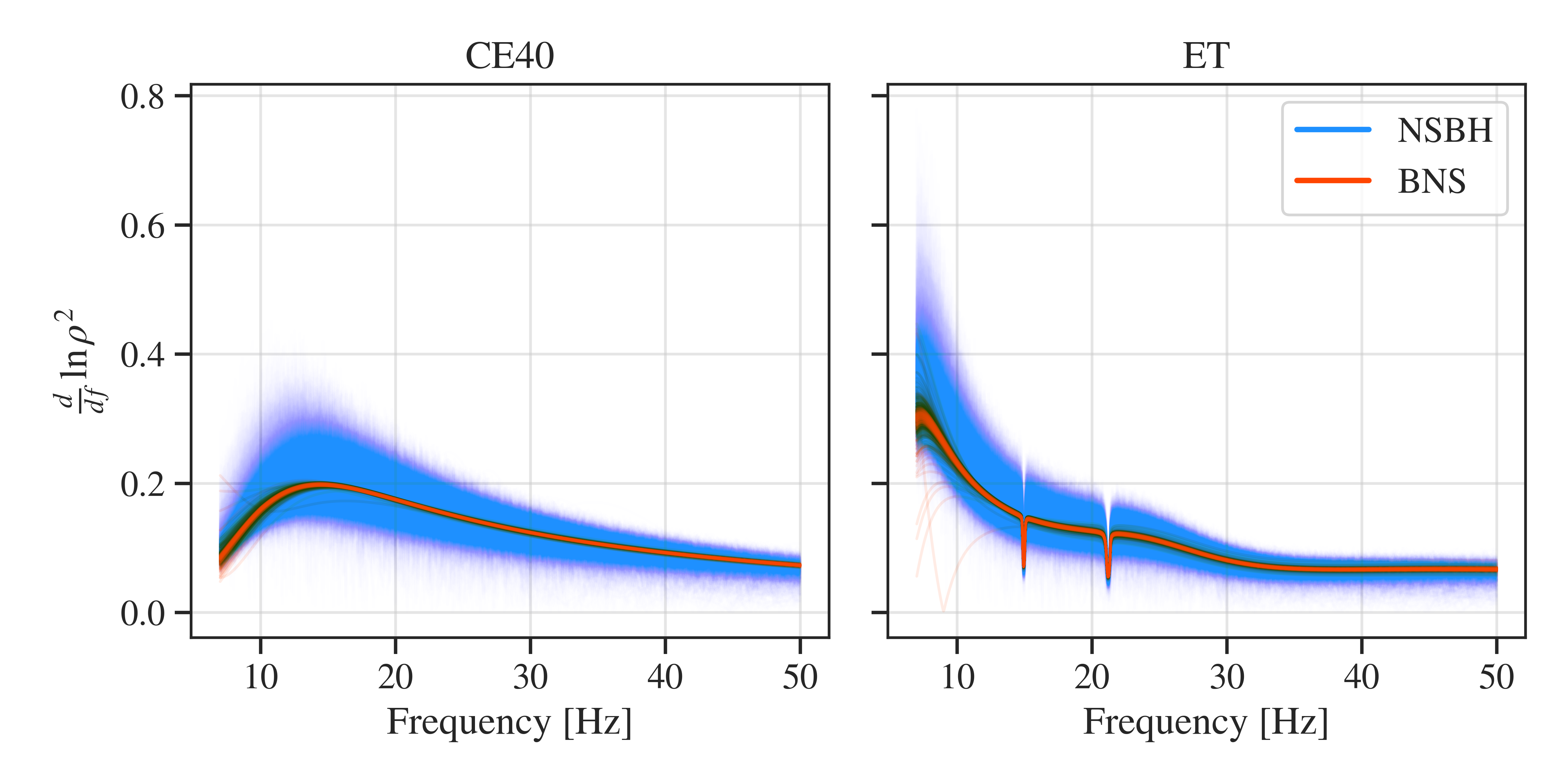
Figure 4: The SNR-squared integrand, normalized by the SNR square, as a frequency function for a simulated population of BNS and NSBH systems in the CE40 detector and in one of the ET detectors.

To understand the underlying reasons for the observed behaviour, we plot in Fig. 4 the normalized differential SNR-squared

$$\frac{d\ln\rho^{2}}{df}=\frac{1}{\rho^{2}}\frac{|\tilde{h}(f)|^{2}}{S_{n}(f)}$$ (6)

for 1000 events picked randomly from the population of BNS and BHNS systems using gwbench [47]. Here, $S_{n}(f)$ represents the design noise curve of each detector, and $\tilde{h}(f)$ is the GW signal in the frequency domain. The plot thus shows the fractional contribution to the SNR as a function of frequency.

We observe that, for the CE40 detector, the dominant contribution to the $d\ln\rho^{2}/df$, for both BNS and BHNS systems arises in the 10–20 Hz frequency range. The BHNS systems (blue curves) show a larger variability in $d\ln\rho^{2}/df$ than the BNS systems (red curves) due to the broader mass distribution of the BHNS population and the presence of higher-order multipoles in the waveform used to describe them [48]. In the case of the ET detector, the dominant contribution to $d\ln\rho^{2}/df$ comes from even lower frequencies, as expected, given its greater sensitivity in the sub-10 Hz regime, where the signal spends more time. This enables ET to capture a larger portion of the signal’s inspiral.

As the GW amplitude decreases $\propto f^{-7/6}$ and the $S_{n}(f)$ remains relatively flat beyond 20 Hz (up to about 500 Hz), the differential SNR-squared decreases steadily for both types of systems, thereby having a lesser impact on the Welch PSD estimate.

III Analysis Setup

Parameter	Symbol	GW150914	GW190521
Mass ratio	$q$	0.98	0.95
Source-frame total mass $(M_{\odot})$	$M_{T}$	63.05	210.51
Primary spin magnitude	$\chi_{1}$	0.58	0.83
Secondary spin magnitude	$\chi_{2}$	0.43	0.96
Primary tilt (rad)	$\theta_{1}$	2.49	1.56
Secondary tilt (rad)	$\theta_{2}$	0.78	1.96
Azimuthal inter-spin angle (rad)	$\phi_{12}$	3.98	0.23
Azimuthal precession cone angle (rad)	$\phi_{\mathrm{JL}}$	0.06	0.36
Effective aligned spin	$\chi_{\textrm{eff }}$	-0.08	0.19
Effective precessing spin	$\chi_{p}$	0.35	0.83
Azimuth (rad)	$\phi$	2.20	1.06
Polarization angle (rad)	$\psi$	0.68	1.27
Right ascension (rad)	$\alpha$	2.16	4.39
Declination (rad)	$\delta$	-1.25	0.85
Inclination angle (rad)	$\theta_{JN}$	2.55	2.09

Table 1: Maximum likelihood parameter values for the simulated systems, derived from the GW150914 and GW190521 posteriors as obtained by Islam et al. [49].

This section describes the setup used to simulate and analyse GW signals in the presence of foreground noise. We begin by outlining the parameters and configurations of the simulated signals, which are based on BBH mergers, GW150914 and GW190521. We then detail the inference settings, including the waveform models, prior choices, and sampler configurations used to perform parameter estimation.

III.1 Simulated Signals

We simulate two types of BBH signals to explore how foreground noise affects binary PE: GW150914-like and GW190521-like, where the former represents a typical Pop-III BBH system [36], and the latter a typical IMBH binary system. All source parameters, except for the luminosity distance $D_{L}$, are set to the maximum-likelihood values from the publicly available posterior samples for these events, as reported by Islam et al. [49] using the NRSur7dq4 waveform model (See Table 1).

The GW150914-like systems are placed at redshifts $z=5,10,15,20,25$, such that the redshifted detector-frame total mass, $M_{T}(1+z)$, lies between $378M_{\odot}$ and $1638M_{\odot}$. Since larger binary masses reduce the frequency at the merger, effectively limiting the signal’s bandwidth, these systems spend most of their evolution in the lower-frequency bands, where the impact of the foreground noise is most significant. Similarly, the GW190521-like systems are placed at redshifts $z=1,2,4,6,8$. These simulated signals are added into multiple noise realisations (with and without foreground noise) to create multiple datasets, each of which is analyzed with the inference settings described below.

III.2 Inference Settings

Data and waveform model:

We conduct full Bayesian PE on 16 seconds of simulated data around the target signal using Bilby. Both the signal simulation and PE use the NRSur7dq4 waveform model [50] , which is trained on quasi-spherical BBH simulations from the SXS catalogue [51], with mass ratios $q=m_{1}/m_{2}\leq 4$ and dimensionless spins $\chi_{i}\leq 0.8$. However, the models work well even when extrapolated outside their training parameter space range up to $q$ = 6.

Priors:

Consistent with Abbott et al. [52], we adopt uniform priors on spin magnitudes ($0\leq\chi_{1,2}\leq 0.99$) and detector-frame component masses $m_{i}(1+z)$, assuming isotropic distributions for spin orientations, sky location, and binary orientation parameters ($\iota,\phi$). The priors on the component masses are subject to the following constraints: (i) the mass ratio $q$ satisfies $1/6\leq q\leq 1$; (ii) the total mass $M_{T}(1+z)$ exceeds $100M_{\odot}$; and (iii) the chirp mass $\mathcal{M}_{c}(1+z)$ lies within the range $60M_{\odot}\leq\mathcal{M}_{c}(1+z)\leq 400M_{\odot}$.

For the luminosity distance, we assume a uniform prior in the source frame, and flat $\Lambda$CDM cosmology with Hubble parameter $H_{0}=67.9\,\mathrm{km}\,\mathrm{s}^{-1}\,\mathrm{Mpc}^{-1}$ and dark matter density $\Omega_{m}=0.3065$, as in Romero-Shaw et al. [53], Abbott et al. [52], and $D_{L}$ prior constrained between 1 Gpc and 500 Gpc.

Frequency settings:

All analyses are performed with a lower frequency cutoff of $f_{\mathrm{low}}=7$ Hz across the detector network. This is also the reference frequency at which all spin posterior distributions are evaluated.

Sampler settings:

Posterior sampling is performed using the dynesty sampler in its static configuration, with 1024 live points [54]. We employ random walks for sampling, with a minimum of 100 and a maximum of 10,000 MCMC steps. The number of random walk steps in each chain is at least 50 times the autocorrelation length (nact). The sampling process continues until the unaccounted evidence fraction, dlogz, reaches 0.1.

IV Results

This section assesses the impact of foreground noise on the PE of GW190521-like and GW150914-like signals. In particular, we show the posteriors for the source-frame component masses, $m_{1}$ and $m_{2}$, effective aligned-spin parameter $\chi_{\mathrm{eff}}$ , and redshift $z$. These distributions are compared for the cases where the data contains no foreground noise (Gaussian), foreground noise corresponding to Population-A (Pop-A), and foreground noise corresponding to Population-B (Pop-B).

As BBHs that form dynamically in active galactic nuclei can produce electromagnetic counterparts (see Graham et al. [58] and references therein), accurate localization of these binaries is required for astrophysical and cosmological analyses. Thus, we also present the posterior distributions on the right ascension $(\alpha)$ and the cosine of declination $(\mathrm{cos}\,\delta)$ for all the scenarios.

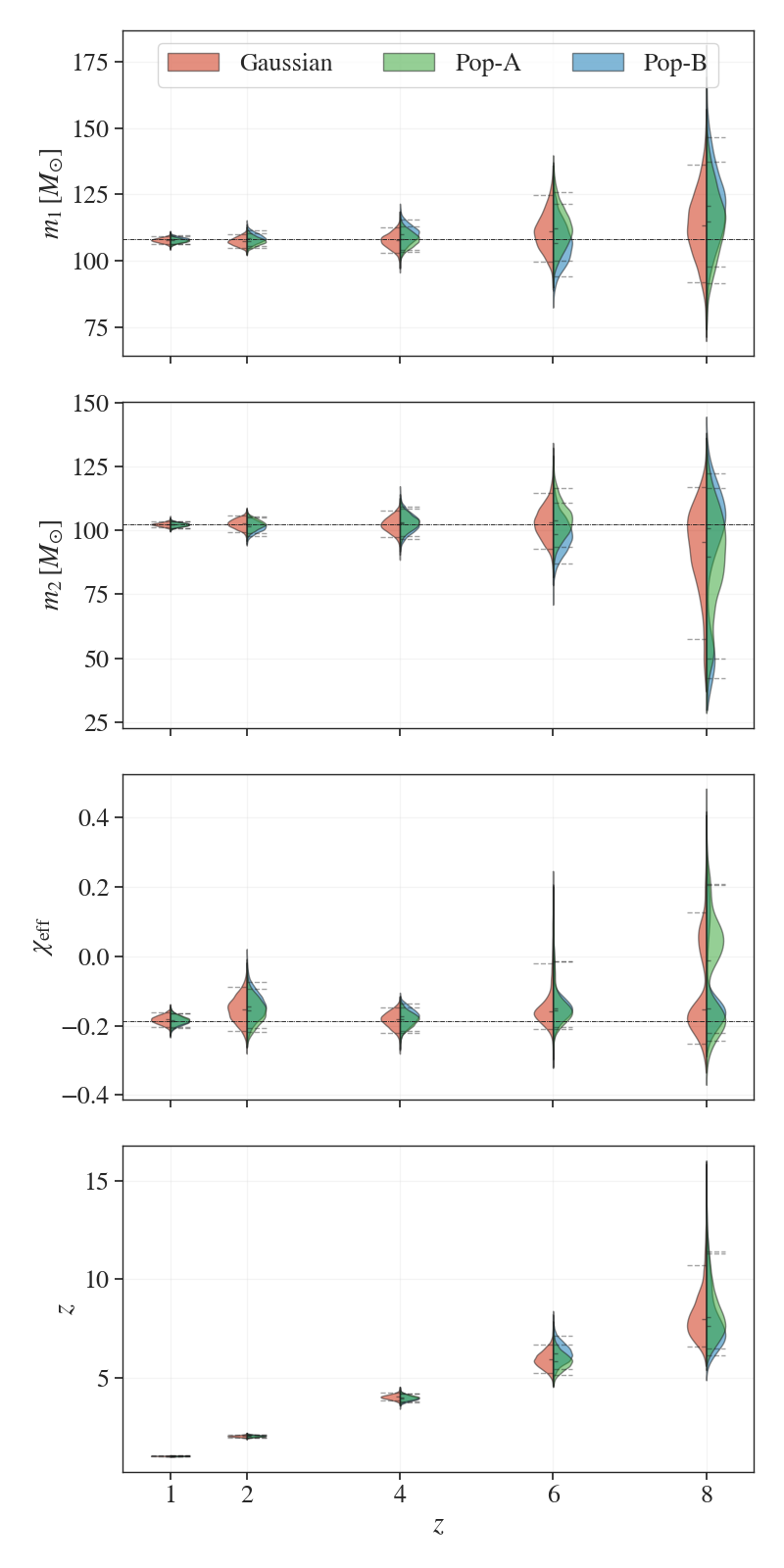
Figure 5: The posterior distribution of the source-frame total mass, mass ratio, and the effective spin parameter for GW190521-like events at different redshifts injected in gaussian noise and foreground noise corresponding to Pop-A and Pop-B. The small solid horizontal line indicates the median of the corresponding distribution, and the dotted horizontal lines show the respective $90\%$ credible interval. The dashed black line shows the true values for $m_{1}$, $m_{2}$, and $\chi_{\rm eff}$.

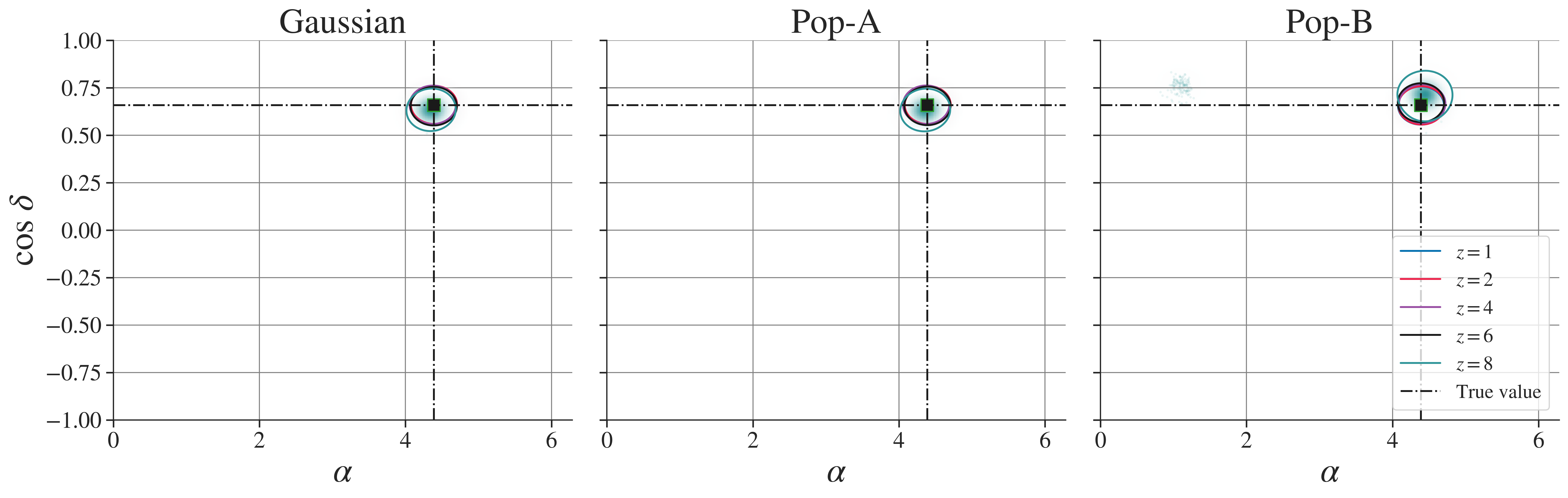
Figure 6: The inferred $90\%$ credible intervals for the right ascension and cosine of declination for GW190521-like IMBHs.

IV.1 GW190521-like signals

Figure 5 shows the posteriors for $m_{1}$, $m_{2}$, $\chi_{\rm eff}$, and $z$, for GW190521-like events in the three foreground noise scenarios considered in this study. The SNRs for the Gaussian and the Pop-A scenarios are similar for all events, but they reduce by $5\%$-$10\%$ for Pop-B. Across the redshift range explored, we find that the posteriors for the signal parameters for the Gaussian and the Pop-A cases are alike, with the maximum Jensen Shannon divergence (JSD) value being 0.008 nat, indicating that the precision of PE is largely unaffected by differences in the assumed population model.

When comparing the Gaussian and the Pop-B scenarios, we find the posteriors to be broadly consistent, with $\mathrm{\acs{jsd}^{\rm Pop-B}_{\rm Gaussian}\in[0.001,0.08]}$ nat. While the posteriors are expected to be broader for the Pop-B scenario and are seen to deviate slightly from the Gaussian case, the true value lies within the $90\%$ credible interval in all the cases.

Additionally, we observe that the $\chi_{\mathrm{eff}}$ posteriors for the $z=2$ system are broader than those for the $z>2$ systems. This broadening exists for the Gaussian case as well. It persists even when the $z=2$ event is injected into different data segments, indicating that foreground noise does not drive the effect. In fact, the effect of foreground noise is minimal for this event, with $\mathrm{\acs{jsd}^{\rm Pop-B}_{\rm Gaussian}=0.08}$ nat. We investigate the broadening of $\chi_{\rm eff}$ for this event in Appendix B.

Finally, Figure 6 displays the inferred posterior distributions for $\alpha$ and cos$\,\delta$ across different redshifts and foreground noise scenarios. The sky-localization posteriors are consistent across all cases, showing broadening for the Pop-B scenario but no significant deviations. Even in the lowest SNR case, corresponding to the $z=8$ event with an SNR $\sim 14$ for the Pop-B scenario, the presence of high foreground noise from CBCs does not bias the sky-localization. This suggests that sky-localization accuracy remains robust, even in scenarios with high merger rates.

IV.2 GW150914-like signals

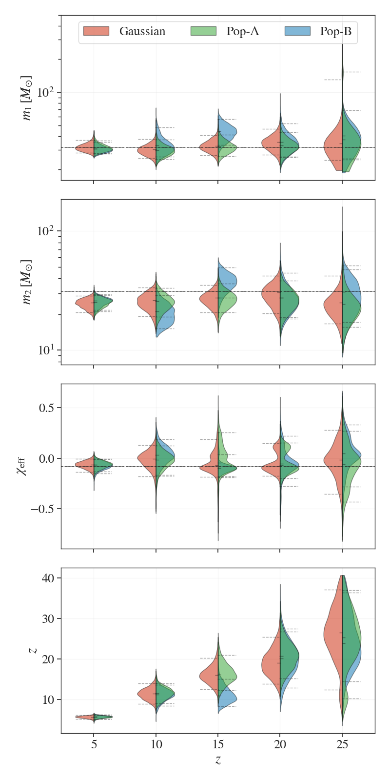
Figure 7: Same as Fig. 5 but for GW150914-like BBHs at different redshifts.

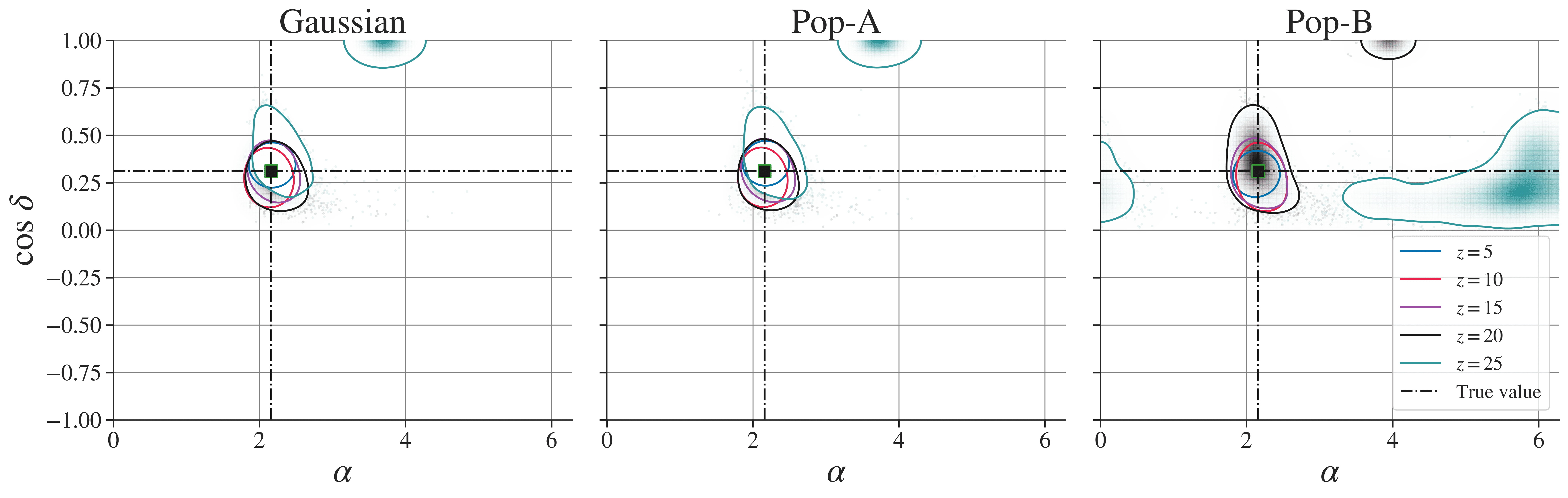
Figure 8: Same as Fig. 6 but for GW150914-like BBHs.

Figure 7 shows the posterior probability distributions for $m_{1,2}$, $\chi_{\rm eff}$, and $z$ for GW150914-like events, representing Pop-III BBHs. In both the Gaussian and Pop-A scenarios, the SNRs are similar, whereas for Pop-B, they are reduced by approximately $15\%$–$20\%$. Consequently, the posteriors for Pop-B are generally broader. Notably, the inferred parameter distributions in the Gaussian and Pop-A cases are highly consistent, with a maximum JSD of only $0.02$ nat across all parameters.

In the Pop-B scenario, the posterior distributions remain broadly consistent with those from the Gaussian case, with a median JSD of 0.03. However, for the $z=10$ case, we observe a bias in the measurement of $m_{2}$, where the true value falls outside the $90\%$ credible interval ($\mathrm{JSD}^{\rm Pop-B}_{\rm Gaussian}=0.1$ nat) but remains within the $3\sigma$ credible region, indicating that the bias is not statistically significant. The bias is also seen to reduce when the same event in injected in different time segments. At $z=15$, the deviations from the Gaussian and Pop-A cases are more pronounced, with $\mathrm{JSD}^{\rm Pop-B}_{\rm Gaussian}\in[0.01,0.37]$. While this suggests a larger impact of the foreground noise at this redshift, the true values still lie within the $90\%$ credible intervals. Even under high CBC merger rate conditions, the PE for GW150914-like events at high redshifts is not substantially biased, and although the JSD values suggest differences for certain cases, the true values stay within acceptable statistical bounds.

Figure 8 shows the inferred distributions of sky location parameters $\alpha$ and $\cos\delta$. The inferred posteriors align well with the true values at all redshifts for both the Gaussian and Pop-A cases. However, for the binary at $z=25$, an additional mode appears for both, likely due to the influence of Gaussian noise, as the SNR at this redshift is approximately $13$. In contrast, for Pop-B, the posterior distributions are significantly broader, and the true value falls outside the $90\%$ credible region for the $z=25$ case.

Thus, while a foreground composed of CBCs following median merger rate estimates does not substantially affect source localization, higher merger rate foregrounds degrade both the precision and accuracy of sky localization for GW150914-like events at high redshifts. Although precise localization is essential for electromagnetic follow-up and cosmological studies [59, 60, 61], our results suggest that significant deviations from true values primarily occur for low-SNR, extremely distant events, and are therefore not a major concern.

V Conclusion

This paper investigates the impact of foreground noise generated by overlapping CBC signals in XG GW observatories. Such noise, originating from numerous in-band signals, renders the detector data non-Gaussian and non-stationary and primarily affects low-frequency sensitivity.

Unlike previous studies, we neither subtract non-target GW signals nor develop new joint signal and noise inference methods. Instead, we employ current techniques to (a) quantify the strength of the foreground noise due to different binary populations, (b) identify the frequencies and conditions where this noise is most impactful, (c) assess its effect on GW search sensitivity, and (d) evaluate its influence on binary parameter estimation.

Our analysis considers three scenarios: (a) Gaussian noise coloured by XG design sensitivity curves, (b) Gaussian noise combined with foreground noise from CBCs at median merger rates (Pop-A), and (c) Gaussian noise with foreground noise from CBCs population at higher merger rates (Pop-B). We use the Welch method to estimate the PSD, finding that the PSD can deviate by up to $50\%$ from Gaussian noise levels for Pop-B at sub-30Hz frequency. This can reduce the detector’s horizon reach by $\sim 25\%$.

Given this, we use the state-of-the-art Bayesian inference package Bilby to measure the component source-frame masses $m_{k}$, effective aligned-spin parameter $\chi_{\mathrm{eff}}$ and redshift $z$, used interchangeably with luminosity distance $D_{L}$. We restrict our attention to two different simulated binary populations, namely GW190521-like IMBH mergers up to a redshift of 8 and GW150914-like BBH mergers (representing mergers of black holes from Pop-III stars) up to a redshift of 25.

We find that for both GW190521-like and GW150914-like systems, the posteriors in the Gaussian and Pop-A cases are highly consistent, with JSD values less than 0.01 nat. This demonstrates that foreground noise due to median merger rate estimates does not significantly affect parameter estimation.

However, in the Pop-B case, where the number of signals is higher, we observe a reduction in the SNR by $15\%$–$20\%$ due to the foreground noise. This leads to broader posterior distributions, though biases in parameter estimation remain statistically insignificant (below $3\sigma$). Consequently, we conclude that the foreground noise at high merger rates does not substantially affect the accurate estimation of parameters such as masses, spins, and redshifts. This result is significant as it implies that even in high foreground noise, XG detectors can still provide reliable characterization and inference of high-redshift merger properties without subtracting foreground signals.

We also assess the impact of the foreground noise on sky localization, finding that foreground noise does not substantially degrade accuracy, except at low SNR cases, where mislocalization may occur. This suggests that key science goals, including electromagnetic follow-up and cosmological studies, will not be compromised by foreground noise.

In summary, our findings demonstrate that foreground noise will not significantly affect PE for short-duration, high-mass BBH systems in XG GW detectors, even in the presence of high CBC merger rates. This result suggests that accurate recovery of system properties is achievable without the need for global fit and/or signal subtraction techniques. Looking ahead, expanding this work to include population-level hierarchical analyses will be crucial for verifying that foreground noise does not bias the inference of hyperparameters that characterize high-redshift populations. However, developing faster and more sophisticated parameter inference algorithms tailored to the intricate noise conditions expected in future observatories will be essential for fully realizing the scientific potential of XG GW astronomy.

Appendix A Number of overlapping signals per frequency bin

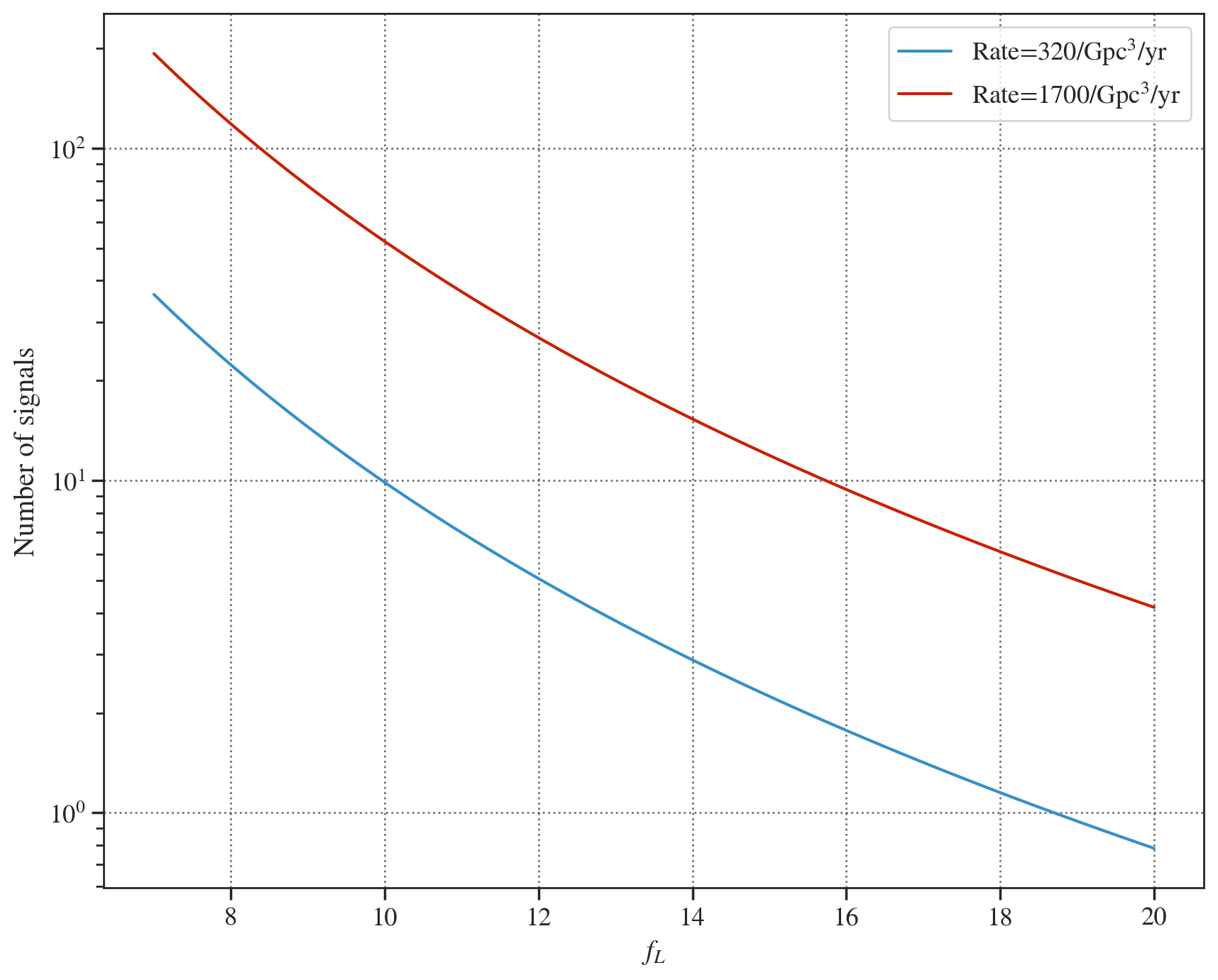
Figure 9: Estimated number of overlapping signals as a function of lower frequency cutoff $f_{L}$ for two local merger rate densities.

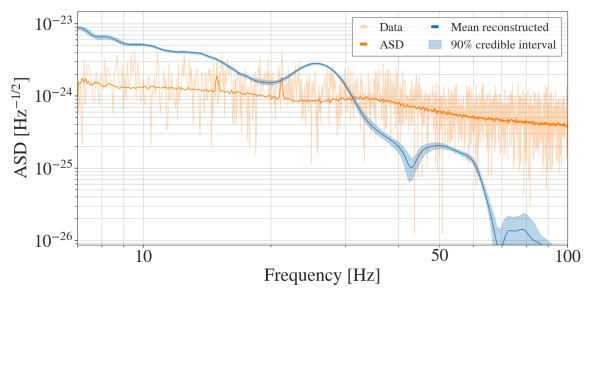
Figure 10: The reconstructed waveform for the GW190521-like IMBH at z=2, with the ASD for ET.

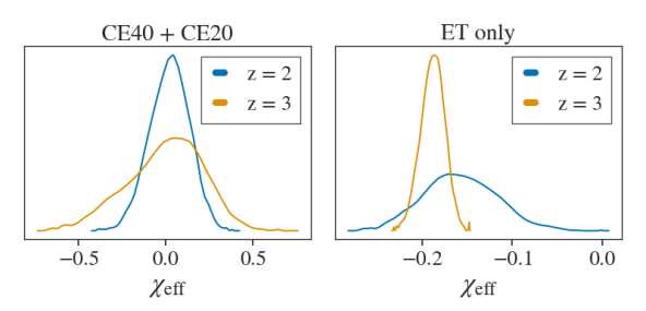
Figure 11: The $\chi_{\rm eff}$ posterior distribution for the $z=2$ and $z=3$ cases in Gaussian noise with CE40 and CE20 detectors, and with only the ET observatory.

We guesstimate the number of overlapping signals per frequency bin as follows.

Consider a binary population with redshifted total mass $M_{T}(1+z)$ and symmetric mass ratio $\eta=m_{1}m_{2}/M_{T}^{2}$. In the Newtonian limit, the duration of a signal starting from a lower frequency cutoff $f_{L}$ is given by

$$\tau_{c}(f_{L})=\frac{5}{256\eta}\frac{GM_{T}(1+z)}{c^{3}}\left(\frac{\pi GM_{T}(1+z)f_{L}}{c^{3}}\right)^{-8/3}.$$ (7)

If the target signal duration is $t$, then the number of signals in the frequency range $[f_{L},f_{L}+1/t]$ is determined by

$$\Delta\tau=\tau_{c}(f_{L})-\tau_{c}(f_{L}+1/t).$$ (8)

Assuming a local merger rate density $\mathcal{R}$ (in units of $\mathrm{Gpc}^{-3}\,\mathrm{yr}^{-1}$) and a horizon volume $V_{H}$ (in Gpc³), the rate of signals per second is

$$\dot{n}=\frac{\mathcal{R}\times V_{H}}{365\times 24\times 60\times 60}.$$ (9)

Thus, the number of signals within $\Delta\tau$ is $\Delta\tau\times\dot{n}$. Figure 9 shows the estimated number of overlapping GW signals as a function of $f_{L}$ for two different local merger rate densities: $320\,\mathrm{Gpc}^{-3}\,\mathrm{yr}^{-1}$ (blue curve) and $1700\,\mathrm{Gpc}^{-3}\,\mathrm{yr}^{-1}$ (red curve). We assume that the system’s considered have $M_{T}(1+z)=2M_{\odot}$ and $\eta=0.25$, thereby giving the upper limit to the number of overlapping signals. As $f_{L}$ increases, overlapping signals decrease for both merger rate densities. This trend is expected because higher $f_{L}$ values correspond to shorter signal durations, which results in fewer opportunities for signals to overlap within a given frequency bin.

Appendix B Investigating $\chi_{\rm eff}$ posterior for GW190521-like event at z=2

In Section IV.1, we saw that the effect of foreground noise on PE for GW190521-like IMBHs is minimal. However, the posterior distribution obtained for $\chi_{\rm eff}$ for the $z=2$ case was considerably broader than those for $z>2$ events, which is unexpected as the SNR of the latter events is lower than that of $z=2$. As seen in Fig. 10, the instrument line in ET detectors intersects the reconstructed waveform just before the merger for the z=2 case. For $z>2$ events, the merger happens below $20$ Hz and is unaffected by this feature. To corroborate that the issue occurs due to the noise feature, we re-perform parameter estimation on the $z=2$ and the $z=3$ cases with CE40 and CE20 (no noise feature), and with ET only (with noise feature), in Gaussian noise. This is presented in Fig. 11. We see that, unlike Fig. 5, the posterior distribution of $\chi_{\rm eff}$ becomes broader, going from $z=2$ to $z=3$, when the events are injected in CE40 and CE20, following our expectation. But when the event is simulated in ET only, the $\chi_{\rm eff}$ is measured more precisely for the $z=3$ case.

References

- Hild et al. [2008] S. Hild, S. Chelkowski, and A. Freise, Pushing towards the ET sensitivity using ’conventional’ technology, arXiv:0810.0604 [gr-qc] (2008).
- Punturo et al. [2010] M. Punturo et al., The Einstein Telescope: A third-generation gravitational wave observatory, Class. Quant. Grav. 27, 194002 (2010).
- Hild et al. [2011] S. Hild et al., Sensitivity Studies for Third-Generation Gravitational Wave Observatories, Class. Quant. Grav. 28, 094013 (2011), arXiv:1012.0908 [gr-qc] .
- Reitze et al. [2019] D. Reitze et al., Cosmic Explorer: The U.S. Contribution to Gravitational-Wave Astronomy beyond LIGO, Bull. Am. Astron. Soc. 51, 035 (2019), arXiv:1907.04833 [astro-ph.IM] .
- Evans et al. [2021] M. Evans et al., A Horizon Study for Cosmic Explorer: Science, Observatories, and Community, arXiv:2109.09882 [astro-ph.IM] (2021).
- Evans et al. [2023] M. Evans et al., Cosmic Explorer: A Submission to the NSF MPSAC ngGW Subcommittee, arXiv:2306.13745 [astro-ph.IM] (2023).
- Branchesi et al. [2023] M. Branchesi et al., Science with the Einstein Telescope: a comparison of different designs, JCAP 07, 068, arXiv:2303.15923 [gr-qc] .
- Gupta et al. [2023a] I. Gupta et al., Characterizing Gravitational Wave Detector Networks: From A♯ to Cosmic Explorer, arXiv:2307.10421 [gr-qc] (2023a).
- Borhanian and Sathyaprakash [2022] S. Borhanian and B. S. Sathyaprakash, Listening to the Universe with Next Generation Ground-Based Gravitational-Wave Detectors, arXiv:2202.11048 [gr-qc] (2022).
- Iacovelli et al. [2022] F. Iacovelli, M. Mancarella, S. Foffa, and M. Maggiore, Forecasting the Detection Capabilities of Third-generation Gravitational-wave Detectors Using GWFAST, Astrophys. J. 941, 208 (2022), arXiv:2207.02771 [gr-qc] .
- Gupta et al. [2023b] I. Gupta, S. Borhanian, A. Dhani, D. Chattopadhyay, R. Kashyap, V. A. Villar, and B. S. Sathyaprakash, Neutron star-black hole mergers in next generation gravitational-wave observatories, Phys. Rev. D 107, 124007 (2023b), arXiv:2301.08763 [gr-qc] .
- Relton et al. [2022] P. Relton, A. Virtuoso, S. Bini, V. Raymond, I. Harry, M. Drago, C. Lazzaro, A. Miani, and S. Tiwari, Addressing the challenges of detecting time-overlapping compact binary coalescences, Phys. Rev. D 106, 104045 (2022), arXiv:2208.00261 [gr-qc] .
- Umstatter et al. [2005] R. Umstatter, N. Christensen, M. Hendry, R. Meyer, V. Simha, J. Veitch, S. Vigeland, and G. Woan, LISA source confusion: Identification and characterization of signals, Class. Quant. Grav. 22, S901 (2005), arXiv:gr-qc/0503121 .
- Wu and Nitz [2023] S. Wu and A. H. Nitz, Mock data study for next-generation ground-based detectors: The performance loss of matched filtering due to correlated confusion noise, Phys. Rev. D 107, 063022 (2023), arXiv:2209.03135 [astro-ph.IM] .
- Johnson et al. [2024] A. D. Johnson, K. Chatziioannou, and W. M. Farr, Source confusion from neutron star binaries in ground-based gravitational wave detectors is minimal, Phys. Rev. D 109, 084015 (2024), arXiv:2402.06836 [gr-qc] .
- Chandra [2024] K. Chandra, gwforge: A user-friendly package to generate gravitational-wave mock data, arXiv e-prints , arXiv:2407.21109 (2024), arXiv:2407.21109 [gr-qc] .
- Antonelli et al. [2021] A. Antonelli, O. Burke, and J. R. Gair, Noisy neighbours: inference biases from overlapping gravitational-wave signals, Mon. Not. Roy. Astron. Soc. 507, 5069 (2021), arXiv:2104.01897 [gr-qc] .
- Reali et al. [2022] L. Reali, A. Antonelli, R. Cotesta, S. Borhanian, M. Çalışkan, E. Berti, and B. S. Sathyaprakash, The impact of confusion noise on golden binary neutron-star events in next-generation terrestrial observatories, arXiv:2209.13452 [gr-qc] (2022).
- Allen et al. [2012] B. Allen, W. G. Anderson, P. R. Brady, D. A. Brown, and J. D. E. Creighton, FINDCHIRP: An Algorithm for detection of gravitational waves from inspiraling compact binaries, Phys. Rev. D 85, 122006 (2012), arXiv:gr-qc/0509116 .
- Cornish and Littenberg [2015] N. J. Cornish and T. B. Littenberg, BayesWave: Bayesian Inference for Gravitational Wave Bursts and Instrument Glitches, Class. Quant. Grav. 32, 135012 (2015), arXiv:1410.3835 [gr-qc] .
- Pizzati et al. [2022] E. Pizzati, S. Sachdev, A. Gupta, and B. Sathyaprakash, Toward inference of overlapping gravitational-wave signals, Phys. Rev. D 105, 104016 (2022), arXiv:2102.07692 [gr-qc] .
- Samajdar et al. [2021] A. Samajdar, J. Janquart, C. Van Den Broeck, and T. Dietrich, Biases in parameter estimation from overlapping gravitational-wave signals in the third-generation detector era, Phys. Rev. D 104, 044003 (2021), arXiv:2102.07544 [gr-qc] .
- Jani et al. [2019] K. Jani, D. Shoemaker, and C. Cutler, Detectability of Intermediate-Mass Black Holes in Multiband Gravitational Wave Astronomy, Nature Astron. 4, 260 (2019), arXiv:1908.04985 [gr-qc] .
- Chandra et al. [2024a] K. Chandra, A. Pai, S. H. W. Leong, and J. Calderón Bustillo, Impact of Bayesian priors on the inferred masses of quasicircular intermediate-mass black hole binaries, Phys. Rev. D 109, 104031 (2024a), arXiv:2309.01683 [gr-qc] .
- Ng et al. [2021] K. K. Y. Ng, S. Vitale, W. M. Farr, and C. L. Rodriguez, Probing multiple populations of compact binaries with third-generation gravitational-wave detectors, Astrophys. J. Lett. 913, L5 (2021), arXiv:2012.09876 [astro-ph.CO] .
- Aasi et al. [2015] J. Aasi et al. (LIGO Scientific), Advanced LIGO, Class. Quant. Grav. 32, 074001 (2015), arXiv:1411.4547 [gr-qc] .
- Acernese et al. [2015] F. Acernese et al. (VIRGO), Advanced Virgo: a second-generation interferometric gravitational wave detector, Class. Quant. Grav. 32, 024001 (2015), arXiv:1408.3978 [gr-qc] .
- Chandra et al. [2021] K. Chandra, V. Villa-Ortega, T. Dent, C. McIsaac, A. Pai, I. W. Harry, G. S. C. Davies, and K. Soni, An optimized PyCBC search for gravitational waves from intermediate-mass black hole mergers, Phys. Rev. D 104, 042004 (2021), arXiv:2106.00193 [gr-qc] .
- Nitz et al. [2023] A. H. Nitz, S. Kumar, Y.-F. Wang, S. Kastha, S. Wu, M. Schäfer, R. Dhurkunde, and C. D. Capano, 4-OGC: Catalog of Gravitational Waves from Compact Binary Mergers, Astrophys. J. 946, 59 (2023), arXiv:2112.06878 [astro-ph.HE] .
- Abbott et al. [2023a] R. Abbott et al. (KAGRA, VIRGO, LIGO Scientific), GWTC-3: Compact Binary Coalescences Observed by LIGO and Virgo during the Second Part of the Third Observing Run, Phys. Rev. X 13, 041039 (2023a), arXiv:2111.03606 [gr-qc] .
- Reali et al. [2024] L. Reali, R. Cotesta, A. Antonelli, K. Kritos, V. Strokov, and E. Berti, Intermediate-mass black hole binary parameter estimation with next-generation ground-based detector networks (2024), arXiv:2406.01687 [gr-qc] .
- Kinugawa et al. [2014] T. Kinugawa, K. Inayoshi, K. Hotokezaka, D. Nakauchi, and T. Nakamura, Possible Indirect Confirmation of the Existence of Pop III Massive Stars by Gravitational Wave, Mon. Not. Roy. Astron. Soc. 442, 2963 (2014), arXiv:1402.6672 [astro-ph.HE] .
- Belczynski et al. [2017] K. Belczynski, T. Ryu, R. Perna, E. Berti, T. L. Tanaka, and T. Bulik, On the likelihood of detecting gravitational waves from Population III compact object binaries, Mon. Not. Roy. Astron. Soc. 471, 4702 (2017), arXiv:1612.01524 [astro-ph.HE] .
- Tanikawa et al. [2022] A. Tanikawa, T. Yoshida, T. Kinugawa, A. A. Trani, T. Hosokawa, H. Susa, and K. Omukai, Merger Rate Density of Binary Black Holes through Isolated Population I, II, III and Extremely Metal-poor Binary Star Evolution, Astrophys. J. 926, 83 (2022), arXiv:2110.10846 [astro-ph.HE] .
- Ng et al. [2022] K. K. Y. Ng, G. Franciolini, E. Berti, P. Pani, A. Riotto, and S. Vitale, Constraining High-redshift Stellar-mass Primordial Black Holes with Next-generation Ground-based Gravitational-wave Detectors, Astrophys. J. Lett. 933, L41 (2022), arXiv:2204.11864 [astro-ph.CO] .
- Santoliquido et al. [2023] F. Santoliquido, M. Mapelli, G. Iorio, G. Costa, S. C. O. Glover, T. Hartwig, R. S. Klessen, and L. Merli, Binary black hole mergers from Population III stars: uncertainties from star formation and binary star properties, Mon. Not. Roy. Astron. Soc. 524, 307 (2023), [Erratum: Mon.Not.Roy.Astron.Soc. 528, 954–962 (2024)], arXiv:2303.15515 [astro-ph.GA] .
- Abac et al. [2024] A. G. Abac et al. (LIGO Scientific, Virgo,, KAGRA, VIRGO), Observation of Gravitational Waves from the Coalescence of a 2.5–4.5 M ⊙ Compact Object and a Neutron Star, Astrophys. J. Lett. 970, L34 (2024), arXiv:2404.04248 [astro-ph.HE] .
- Chandra et al. [2024b] K. Chandra, I. Gupta, R. Gamba, R. Kashyap, D. Chattopadhyay, A. Gonzalez, S. Bernuzzi, and B. S. Sathyaprakash, Everything everywhere all at once: A detailed study of GW230529, ArXiv (2024b), arXiv:2405.03841 [astro-ph.HE] .
- Vitale et al. [2024] S. Vitale, L. Barsotti, E. Berger, D. Brown, A. Corsi, M. Evans, S. Fairhurst, M. Landry, and B. Sathyaprakash, Network configurations for mpsac, https://github.com/cosmic-explorer/mpsac_detector_networks/blob/main/doc/Network_configurations_for_MPSAC.pdf (2024), accessed: 2024-09-02.
- Ashton et al. [2019] G. Ashton et al., BILBY: A user-friendly Bayesian inference library for gravitational-wave astronomy, Astrophys. J. Suppl. 241, 27 (2019), arXiv:1811.02042 [astro-ph.IM] .
- Chandra [2024] K. Chandra, Gwforge: A lightweight code to generate mock gravitational wave detector data, https://github.com/koustavchandra/gwforge (2024), accessed: 2024-05-14.
- Abbott et al. [2023b] R. Abbott et al. (KAGRA, VIRGO, LIGO Scientific), Population of Merging Compact Binaries Inferred Using Gravitational Waves through GWTC-3, Phys. Rev. X 13, 011048 (2023b), arXiv:2111.03634 [astro-ph.HE] .
- Madau and Dickinson [2014] P. Madau and M. Dickinson, Cosmic Star Formation History, Ann. Rev. Astron. Astrophys. 52, 415 (2014), arXiv:1403.0007 [astro-ph.CO] .
- Dietrich et al. [2019] T. Dietrich, A. Samajdar, S. Khan, N. K. Johnson-McDaniel, R. Dudi, and W. Tichy, Improving the NRTidal model for binary neutron star systems, Phys. Rev. D 100, 044003 (2019), arXiv:1905.06011 [gr-qc] .
- Pratten et al. [2021] G. Pratten et al., Computationally efficient models for the dominant and subdominant harmonic modes of precessing binary black holes, Phys. Rev. D 103, 104056 (2021), arXiv:2004.06503 [gr-qc] .
- Usman et al. [2016] S. A. Usman et al., The PyCBC search for gravitational waves from compact binary coalescence, Class. Quant. Grav. 33, 215004 (2016), arXiv:1508.02357 [gr-qc] .
- Borhanian [2021] S. Borhanian, GWBENCH: a novel Fisher information package for gravitational-wave benchmarking, Class. Quant. Grav. 38, 175014 (2021), arXiv:2010.15202 [gr-qc] .
- Gupta [2024] I. Gupta, Inferring Small Neutron Star Spins with Neutron Star–Black Hole Mergers, Astrophys. J. 970, 12 (2024), arXiv:2402.07075 [astro-ph.HE] .
- Islam et al. [2023] T. Islam, A. Vajpeyi, F. H. Shaik, C.-J. Haster, V. Varma, S. E. Field, J. Lange, R. O’Shaughnessy, and R. Smith, Analysis of GWTC-3 with fully precessing numerical relativity surrogate models, arXiv e-prints , arXiv:2309.14473 (2023), arXiv:2309.14473 [gr-qc] .
- Varma et al. [2019] V. Varma, S. E. Field, M. A. Scheel, J. Blackman, D. Gerosa, L. C. Stein, L. E. Kidder, and H. P. Pfeiffer, Surrogate models for precessing binary black hole simulations with unequal masses, Phys. Rev. Research. 1, 033015 (2019), arXiv:1905.09300 [gr-qc] .
- Boyle et al. [2019] M. Boyle et al., The SXS Collaboration catalog of binary black hole simulations, Class. Quant. Grav. 36, 195006 (2019), arXiv:1904.04831 [gr-qc] .
- Abbott et al. [2021] R. Abbott et al. (LIGO Scientific, Virgo), GWTC-2: Compact Binary Coalescences Observed by LIGO and Virgo During the First Half of the Third Observing Run, Phys. Rev. X 11, 021053 (2021), arXiv:2010.14527 [gr-qc] .
- Romero-Shaw et al. [2020] I. M. Romero-Shaw et al., Bayesian inference for compact binary coalescences with bilby: validation and application to the first LIGO–Virgo gravitational-wave transient catalogue, Mon. Not. Roy. Astron. Soc. 499, 3295 (2020), arXiv:2006.00714 [astro-ph.IM] .
- Speagle [2020] J. S. Speagle, dynesty: a dynamic nested sampling package for estimating Bayesian posteriors and evidences, Mon. Not. Roy. Astron. Soc. 493, 3132 (2020), arXiv:1904.02180 [astro-ph.IM] .
- Racine [2008] E. Racine, Analysis of spin precession in binary black hole systems including quadrupole-monopole interaction, Phys. Rev. D 78, 044021 (2008), arXiv:0803.1820 [gr-qc] .
- Ajith et al. [2011] P. Ajith et al., Inspiral-merger-ringdown waveforms for black-hole binaries with non-precessing spins, Phys. Rev. Lett. 106, 241101 (2011), arXiv:0909.2867 [gr-qc] .
- Santamaria et al. [2010] L. Santamaria et al., Matching post-Newtonian and numerical relativity waveforms: systematic errors and a new phenomenological model for non-precessing black hole binaries, Phys. Rev. D 82, 064016 (2010), arXiv:1005.3306 [gr-qc] .
- Graham et al. [2023] M. J. Graham et al., A Light in the Dark: Searching for Electromagnetic Counterparts to Black Hole–Black Hole Mergers in LIGO/Virgo O3 with the Zwicky Transient Facility, Astrophys. J. 942, 99 (2023), arXiv:2209.13004 [astro-ph.HE] .
- Chen et al. [2021] H.-Y. Chen, P. S. Cowperthwaite, B. D. Metzger, and E. Berger, A Program for Multimessenger Standard Siren Cosmology in the Era of LIGO A+, Rubin Observatory, and Beyond, Astrophys. J. Lett. 908, L4 (2021), arXiv:2011.01211 [astro-ph.CO] .
- Gupta [2023] I. Gupta, Using grey sirens to resolve the Hubble–Lemaître tension, Mon. Not. Roy. Astron. Soc. 524, 3537 (2023), arXiv:2212.00163 [gr-qc] .
- Chen et al. [2024] H.-Y. Chen, J. M. Ezquiaga, and I. Gupta, Cosmography with next-generation gravitational wave detectors, Class. Quant. Grav. 41, 125004 (2024), arXiv:2402.03120 [gr-qc] .