LLMs are Highly-Constrained Biophysical Sequence Optimizers

Abstract

Large language models (LLMs) have recently shown significant potential in various biological tasks such as protein engineering and molecule design. These tasks typically involve black-box discrete sequence optimization, where the challenge lies in generating sequences that are not only biologically feasible but also adhere to hard fine-grained constraints. However, LLMs often struggle with such constraints, especially in biological contexts where verifying candidate solutions is costly and time-consuming. In this study, we explore the possibility of employing LLMs as highly-constrained bilevel optimizers through a methodology we refer to as Language Model Optimization with Margin Expectation (LLOME). This approach combines both offline and online optimization, utilizing limited oracle evaluations to iteratively enhance the sequences generated by the LLM. We additionally propose a novel training objective – Margin-Aligned Expectation (MargE) – that trains the LLM to smoothly interpolate between the reward and reference distributions. Lastly, we introduce a synthetic test suite that bears strong geometric similarity to real biophysical problems and enables rapid evaluation of LLM optimizers without time-consuming lab validation. Our findings reveal that, in comparison to genetic algorithm baselines, LLMs achieve significantly lower regret solutions while requiring fewer test function evaluations. However, we also observe that LLMs exhibit moderate miscalibration, are susceptible to generator collapse, and have difficulty finding the optimal solution when no explicit ground truth rewards are available.

1 Introduction

Large language models (LLMs) have recently shown significant promise on various biophysical optimization tasks, such as protein engineering and molecule design. These tasks are often formulated as black-box discrete sequence optimization problems, wherein a solver must attempt to output a discrete sequence $\mathbf{x}\in\mathcal{X}$ that is feasible (i.e., a biologically plausible sequence) and that fulfills a number of strict constraints, such as containing specific motifs. Yet despite their many successes, LLMs often struggle to generate outputs that fulfill hard fine-grained constraints [31]. For instance, recent work indicates that many state-of-the-art LLMs cannot effectively generate text with a fixed number of words [107], a particular prefix [95], or specific keywords [19]. This issue is even more pronounced in biological optimization problems, where constraints such as expressivity or low hydrophobicity are typically more complex and costly to check. Verifying that solution candidates meet these constraints often requires expensive and low throughput laboratory experiments. This lack of data presents a formidable challenge for LLMs, which often struggle to generate appropriately constrained sequences even in the presence of large training corpora.

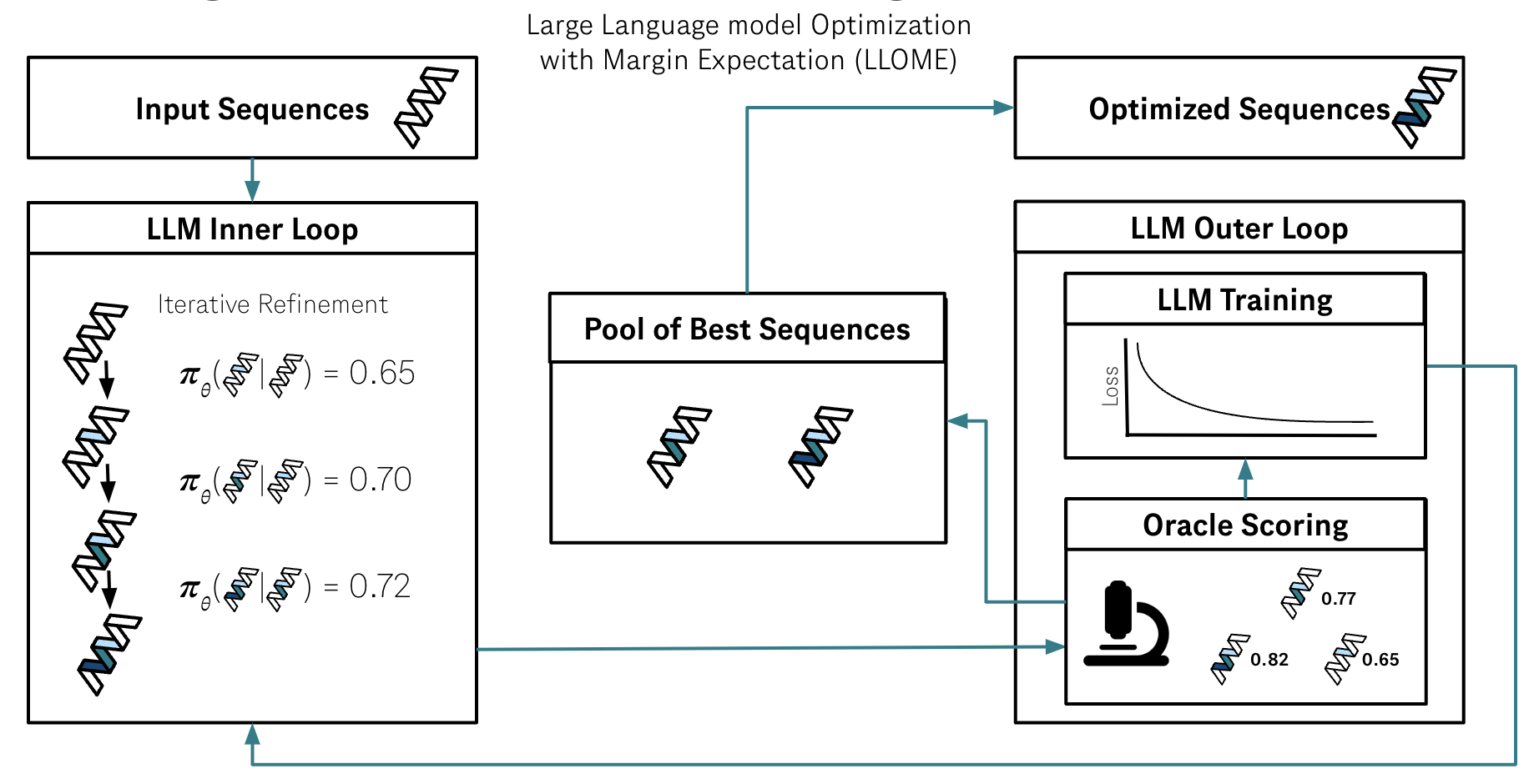
Figure 1: Large language model optimization with Margin Expectation (Llome).

Although some recent work has focused on adapting LLMs to solve black-box optimization problems [54; 84; 1; 15], few include (1) the evaluation of hard constraints, (2) the mixing of offline and online optimization loops, and (3) the use of oracle evaluations. Concerning (1), many commonly studied optimization problems, such as the Rosenbrock function [64], the Ackley function [109], and prompt optimization [106], require only that the optimizer find a solution with a high fitness value, and do not entail strict constraints. When stricter constraints are added, LLMs struggle to generalize without additional aids, such as auxiliary solvers or discriminator models that guide generation [95; 61; 22; 1]. Concerning (2) and (3), laboratory validation often provides a limited number of oracle labels in realistic lab settings. The solver must then be capable of generating, ranking, and filtering its candidates down to a select few that are subsequently sent for oracle evaluation. Importantly, oracle labels are not available during this candidate generation stage. In contrast, many works either use only oracle labels, such as for mathematical optimization problems like linear regression where a solution is easy to verify [64; 106], or simulation-based metrics that bear only a superficial resemblance to the complexity of real-world molecular design tasks [54]. We instead explore LLM capabilities in a more realistic hybrid offline/online setting. During an outer offline optimization loop, we train our optimizer using oracle labels provided by either a seed dataset or the previous round of optimization. In the subsequent online inner optimization loop, our optimizer generates and iteratively refines its candidates without immediate access to the oracle. The optimizer’s top candidates are then scored by the oracle, forming a small labelled training dataset for the next iteration of the outer loop.

In summary, our contributions are as follows:

1. Synthetic Test Suite: Following a long-standing tradition of using synthetic test functions in the optimization literature, we design a suite of closed-form test functions with hard fine-grained constraints that draws upon the characteristics of real biophysical sequence optimization problems. Our test functions have well-characterized solutions, are non-trivial in difficulty, and reflect the non-additive, epistatic nature of biomolecular interactions.

2. Exploring LLMs as Constrained Bilevel Optimizers: We analyze LLMs’ abilities to solve highly-constrained biophysical sequence optimization problems with sparse online feedback via Llome (Large Language model Optimization with Margin Expectation), a method for embedding an LLM in a bilevel optimization loop. In the outer loop, the model is trained on offline data provided by an oracle (e.g., laboratory validation or the evaluation of the synthetic test function). In the inner loop, the model searches for novel and improved sequences without the use of oracle labels. We demonstrate that LLMs often outperform evolutionary baselines, finding lower-regret solutions given a fixed budget of function evaluations. We additionally explore a number of other fundamental questions about LLMs’ optimization capabilities, including whether LLMs can effectively select the best generations, how calibrated LLM predictions are, whether LLMs can iteratively extrapolate at inference-time without access to oracle labels, and when explicit reward values are required during training.

3. Novel LLM Training Objective (MargE): To further explore whether LLMs become better bi-level optimizers when given explicit ground truth rewards, we also propose MargE (Margin-Aligned Expectation), a novel LLM training objective that smoothly interpolates between the target and reference distributions. This objective makes explicit use of the reward margin between the input and the target, which is lacking from common LLM offline training objectives such as supervised finetuning (SFT) and direct preference optimization (DPO). We show that MargE-trained LLMs find the optimal solution more efficiently than DPO- or SFT-trained LLMs.

2 Background

In this work, we consider pre-trained autoregressive large language models $\pi_{\theta}(x)$ parameterized by $\theta$. $\pi_{\theta}$ defines a probability distribution over discrete tokens $x\in\mathcal{V}$ for vocabulary $\mathcal{V}$. We can also define the likelihood of sequences $\mathbf{x}\in\mathcal{V}^{*}$ as $\pi_{\theta}(\mathbf{x})=\prod_{t=1}^{|\mathbf{x}|}\pi_{\theta}(x_{t}|x_{<t})$, where $\mathcal{V}^{*}$ is the set of all concatenations of tokens in $\mathcal{V}$.

Supervised Finetuning (SFT)

After pre-training, LLMs are typically finetuned on some task-specific dataset $\mathcal{D}=\{(\mathbf{x},\mathbf{y})\}$ consisting of pairs of input $\mathbf{x}$ and target $\mathbf{y}$ sequences. During SFT, $\pi_{\theta}$ is trained to minimize the negative conditional log likelihood of examples from $\mathcal{D}$:

$$\theta_{\text{SFT}}=\arg\min_{\theta}-\mathbb{E}_{\mathbf{x},\mathbf{y}\sim\mathcal{D}}\log\pi_{\theta}(\mathbf{y}|\mathbf{x})$$ (1)

Preference Learning

In some settings, LLMs are further trained to align their output distributions to a reward distribution, typically encoded with a reward model $r(\mathbf{x}):\mathcal{V}^{*}\to\mathbb{R}$. This is frequently accomplished with reinforcement learning, where the LLM is trained via a policy gradient method to maximize the expected rewards $\mathbb{E}_{x\sim\mathcal{D},y\sim\pi_{\theta}(\cdot\mid x)}r(x,y)$. The reward model is trained from a dataset of human preferences consisting of triples $(x,y_{w},y_{l})$, where $x$ is a prompt obtained from some offline dataset $\mathcal{X}$ and $y_{w}$ and $y_{l}$ are sampled from the current policy. The initial model is referred to as the reference policy $\pi_{\text{Ref}}$ and $y_{w},y_{l}$ are assigned such that $y_{w}$ is more preferred by human raters than $y_{l}$. More recently, practitioners have added a KL divergence constraint to this objective to prevent the LLM from quickly over-optimizing, yielding an objective known as reinforcement learning from human feedback [RLHF; 116; 94]:

$$\theta_{\text{RLHF}}=\arg\max_{\theta}\underset{\begin{subarray}{c}x\sim\mathcal{X}\\ y\sim\pi_{\theta}(\cdot\mid x)\end{subarray}}{\mathbb{E}}r(x,y)-\beta\mathbb{KL}(\pi_{\theta}\|\pi_{\text{Ref}})$$ (2)

RLHF is commonly trained using Proximal Policy Optimization (PPO), which involves considerable engineering complexity due to the need to train and coordinate four models ($\pi_{\theta}$, $\pi_{\text{Ref}}$, a reward model, and a critic model). Furthermore, RLHF-PPO is particularly sensitive to hyperparameter values and prone to training instabilities [112]. To address some of these issues, an offline version of RLHF known as Direct Preference Optimization [DPO; 79] was proposed. DPO skips reward modeling and directly trains on the preference triples with a contrastive objective:

$$\theta_{\text{DPO}}=\arg\min_{\theta}\underset{x,y_{w},y_{l}\sim\mathcal{D}}{\mathbb{E}}-\log\sigma\left(\beta\log\frac{\pi_{\theta}(y_{w}|x)}{\pi_{\text{Ref}}(y_{w}|x)}-\beta\log\frac{\pi_{\theta}(y_{l}|x)}{\pi_{\text{Ref}}(y_{l}|x)}\right)$$ (3)

DPO often produces models with similar generative quality as RLHF-PPO [79], but involves notable tradeoffs such as faster over-optimization [80] and a distribution mismatch between the training dataset and policy outputs [16; 97]. Nevertheless, DPO has become one of the most prevalent algorithms for offline alignment of LLMs.

We provide further background on past work related to LLMs for optimization in Sec. 5.1.

3 Evaluation

Although considerable effort has been focused on ML efforts for biological discovery in recent years, the rate of benchmark development has not kept pace [98; 92]. While laboratory validation is the gold standard in evaluation, laboratory feedback cycles are slow and involve prohibitive costs of equipment and expert experimentalists. On the other hand, ML algorithm development requires rapid iteration and feedback, usually at a pace that is infeasible with in vitro validation. To close this gap, computational researchers often turn to simulation-based feedback [21]. However, this approach is also subject to steep tradeoffs between fidelity and latency [42; 8; 40].

In this work, we instead propose a class of synthetic test functions that bear strong geometric similarities to real-world biophysical sequence optimization problems. The practice of evaluating optimizers on synthetic test functions is a long-standing one [62], based upon the principle that the test function need only correlate geometrically with the real sequence optimization problem. This approach has the advantage of being easy to verify but difficult to solve while still reflecting key characteristics of the fitness landscapes of real biophysical optimization tasks such as antibody affinity maturation.

To this end, we propose Ehrlich functions, a closed-form family of test functions for sequence optimization benchmarking. Given token vocabulary $\mathcal{V}$ and the set of sequences $\mathcal{V}^{L}$ formed of concatenations of $L$ tokens in $\mathcal{V}$, we first define $\mathcal{F}\subset\mathcal{V}^{L}$, the set of feasible sequences. $\mathcal{F}$ is synthetically defined as the support of a discrete Markov process (DMP), more details of which are given in Appendix A.1. We also define a set of $c$ spaced motifs that represent biophysical constraints in specific regions of a sequence. These motifs are expressed as pairs of vectors $\{(\mathbf{m}^{(1)},\mathbf{s}^{(1)}),\cdots,(\mathbf{m}^{(c)},\mathbf{s}^{(c)})\}$ where $\mathbf{m}^{(i)}\in\mathcal{V}^{k}$, $\mathbf{s}^{(i)}\in\mathbb{Z}_{+}^{k}$, and $k\leq L//c$. An Ehrlich function $f$ then describes the degree to which a sequence $\mathbf{x}\in\mathcal{V}^{L}$ is feasible and possesses all motifs. For $q\in[1,k]$ bits of precision, $f$ is expressed as:

$$f(x)=\begin{cases}\prod_{i=1}^{c}h_{q}(\mathbf{x},\mathbf{m}^{(i)},\mathbf{s}^{(i)})&\text{if }\mathbf{x}\in\mathcal{F}\\ -\infty&\text{otherwise}\end{cases}$$ (4)

The function $h_{q}$ defines the degree to which $\mathbf{x}$ fulfills the constraints, and is defined as follows:

$$h_{q}(\mathbf{x},\mathbf{m}^{(i)},\mathbf{s}^{(i)})=\underset{l<L}{\max}\left(\sum_{j=1}^{k}\mathbbm{1}\left[x_{l+s^{(j)}}=m_{i}^{(j)}\right]\right)//\binom{k}{q}/q$$ (5)

Setting $q=k$ corresponds to a dense signal which increments $h_{q}(\mathbf{x},\mathbf{m}^{(i)},\mathbf{s}^{(i)})$ whenever an additional element of any motif has been fulfilled. We provide additional details in Appendix A.1 about how to ensure that all motifs are jointly satisfiable and that there exists at least one feasible solution that attains the optimal value of 1.0. We also provide further evidence in Appendix A.1 that $f$ is difficult to optimize for a standard evolutionary algorithm, even with small $L$, $k$, and $c$ values.

4 Method

4.1 Bi-level Optimization

We formulate our task as a sequence editing problem, wherein the optimizer intakes a sequence $x$ and must output an edited version $y$ such that $f(y)>f(x)$. Not only is this the setting of common biophysical optimization tasks such as protein design, but LLMs have been shown to be highly effective at iterative refinement [70; 55]. We can then formulate the larger task of adapting LLMs for discrete sequence optimization as a bi-level optimization problem:

$$\max_{\begin{subarray}{c}x\sim\mathcal{X}\\ y\sim\pi_{\theta^{*}}(\cdot\mid x)\end{subarray}}f(y)$$ (6)

$$\text{subject to }\theta^{*}\in \arg\max_{\theta}\underset{\begin{subarray}{c}x\sim\mathcal{X}\\ y\sim\pi_{\theta^{*}}(\cdot\mid x)\end{subarray}}{\mathbb{E}}f(y)$$

The outer loop consists of finding $\theta^{*}$ that maximizes the expected score of sequences $y$ generated by $\pi_{\theta^{*}}$ and the inner loop consists of finding the highest scoring $y$ generated by $\pi_{\theta^{*}}$. To more closely reflect the setting of real-world feedback cycles, we assume access to the oracle scoring function $f$ only in the outer loop. This mimics the case where laboratory validation provides data for the model to be trained on. In the inner loop, the LLM must generate, rank, and filter candidate sequences without immediate access to $f$.

The high level algorithm is given in Algorithm 1. The optimizer is seeded with sequences generated by $n_{0}$ rounds of a genetic algorithm (details in Appendix A.3.3). These initial seeds are scored and used as the training dataset for the first iteration of the outer loop. After training, we enter the inner loop where $\pi_{\theta_{i}}$ generates and iteratively refines new candidate sequences using seeds sampled from its training dataset. During the iterative refinement process, the LLM iteratively ranks its outputs from the previous iterations and edits the highest ranking sequences. To avoid generator collapse, we automatically increment the sampling temperature if the average Hamming distance between the LLM inputs and outputs from the last round fall below a certain threshold. A subsample of $k$ of these refined sequences are scored and used to create the training dataset for the next iteration of the outer loop. As such, no more than $k$ new test function evaluations are required in each optimizer step. To create the training dataset for the next iteration, we adapt PropEn [96], a dataset matching algorithm that implicitly guides the model towards improved regions of the dataset space. The detailed algorithms for DatasetFormatting, IterativeRefinement, and Filter are given in Appendix A.3.

4.2 LLM Training

To train the LLM in the outer loop of the optimization algorithm (step 1 of Algorithm 1), we consider standard offline LLM training algorithms such as supervised finetuning (SFT) and direct preference optimization [79, ;DPO], in addition to a novel objective MargE. We refer to these three variants of Llome as Llome-SFT, Llome-DPO, and Llome-MargE, respectively. We briefly summarize SFT and DPO in Section 2 and describe the rationale for the design of MargE below.

Margin-Aligned Expectation (MargE) Training

Although DPO has recently become a popular preference learning method due to its relative simplicity and competitive results, its offline contrastive objective suffers from a number of drawbacks. Firstly, since DPO optimizes for an off-policy objective, a DPO-trained model rapidly over-optimizes, resulting in generations that decline in quality despite continued improvements in offline metrics [80; 16]. DPO models also fail at ranking text according to human preferences [16] and tend to decrease the probability mass assigned to preferred outputs [71; 81; 29; 72]. As training continues, DPO generations also increase in length, even if the quality of the generations does not necessarily improve [90]. Additionally, when the reference model already performs well on a particular subset of the input domain, DPO cannot achieve the optimal policy without deteriorating performance on that subset [39]. Lastly, DPO does not make use of absolute reward values – instead, it simply assumes that $r(x,y_{w})>r(x,y_{l})$ for all $(x,y_{w},y_{l})$ in the training dataset, but does not use information about how much better $y_{w}$ is than $y_{l}$.

RLHF, on the other hand, involves steep technical complexity and frequently exhibits training instabilities [111; 100; 13]. Hu et al. [39]; Korbak et al. [47] additionally show that RLHF’s objective interpolates between $\pi_{\text{Ref}}$ and a degenerate distribution $\pi^{\delta}$ that places all probability mass on a single reward-maximizing sequence, thereby promoting generator collapse. Indeed, much past work [45; 114; 69] has illustrated the low diversity of RLHF-generated text.

To attempt to resolve these issues, we propose Margin-Aligned Expectation (MargE), a training objective that smoothly interpolates between the reference model $\pi_{\text{Ref}}$ and the optimal policy $\pi^{*}$ and effectively incorporates information about the true reward margin. Like Hu et al. [39], we propose an objective that takes the following general form:

$$\arg\min_{\theta}\left[\mathbb{KL}(\tilde{\pi}_{\theta}\|\pi^{*})+\lambda\mathbb{KL}(\pi_{\text{Ref}}\|\tilde{\pi}_{\theta})\right]$$ (7)

where $\pi^{*}$ is the target reward distribution and $\tilde{\pi}_{\theta}$ is the length-normalized version of $\pi_{\theta}$. If we apply importance sampling and use a Boltzmann function of the reward as $\pi^{*}$, we obtain:

$$\mathcal{L}_{\text{MargE}}(\pi_{\theta},\pi_{\text{Ref}};\mathbb{D}_{x})=\underset{\begin{subarray}{c}x\sim\mathbb{D}_{x},\\ y\sim\pi_{\text{Ref}}(\cdot\mid x)\end{subarray}}{\mathbb{E}}\left[\frac{\pi_{\theta}(y|x)}{\pi_{\text{Ref}}(y|x)}\left(\frac{\log\pi_{\theta}(y|x)}{|y|}-r(x,y)\right)-\lambda\frac{\log\pi_{\theta}(y|x)}{|y|}\right].$$ (8)

For the full derivation, see App. A.2. We additionally devise a reward function for the sequence edit task at hand. It may seem natural to devise a reward function that is exactly equal to the score function $f(x)$. However, the goal of our model is to produce a $y$ with a better score than the input $x$ – therefore, the reward should reflect whether the output is a relative improvement. However, simply setting $r(x,y)=f(y)-f(x)$ would also result in unintended behavior. Since a normalized Bradley-Terry policy is translation-invariant with respect to the rewards, we would have $\pi(y|x)=\pi(y|z)$ for all pairs $x,z\in\mathrm{dom}(f)$ for this particular reward function. (See Lemma 1 for a detailed derivation.) But if $f(x)\neq f(z)$, then $y$ would constitute a greater improvement for one input than the other, which implies that we should not have $\pi(y|x)=\pi(y|z)$.

To avoid this issue, we instead devise a reward function that only rewards a policy for generating a sequence $y$ with higher score than a seed sequence $x$ and assigns 0 reward otherwise:

$$r(x,y)=\begin{cases}f(y)-f(x)&\text{if }f(y)>f(x)\\ 0&\text{otherwise}\end{cases}$$ (9)

In this case, we set $f(x)=0$ for all $x\not\in\mathcal{F}$ to avoid involving $\infty$’s in our calculations. When the policy produces an improved sequence (a sequence with higher score), the reward is equal to the difference in scores. Zero reward is given for sequences with equal or lower score. Notably, this reward function is similar to a margin loss.

5 Experiments

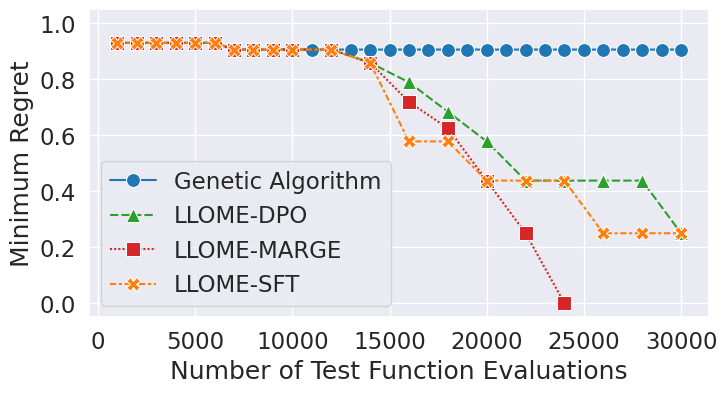
(a) Minimum regret achieved.

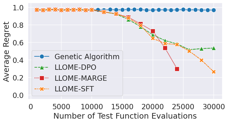
(b) Average regret.

Figure 2: Minimum regret achieved as a function of the number of test function evaluations (2(a)) and average regret of the selected generations in each round of the LLM inner loop (2(b)). The Llome-MargE line ends early because it achieves the optimal solution by 24K test function evaluations. The first 10K test function evaluations of every method correspond to the seeds provided by the genetic algorithm. The shaded regions in (2(b)) represent the mean $\pm$ two standard errors.

Llome Details

We compare the performance of three different variants of Llome (Llome-SFT, Llome-MargE, Llome-DPO) against that of a genetic algorithm. The details of the genetic algorithm are given in Appendix A.3.3 and the training details for SFT, DPO, and MargE are given in Appendix A.4. Each Llome variant is seeded with data from 10 rounds of the genetic algorithm (i.e., $n_{0}=10$). For Llome-MargE and Llome-DPO, one round of SFT is trained before continuing with MargE and DPO training in future iterations. All three variants use the pre-trained model Pythia 2.8B [9] as the base model. During the Train step of each iteration of Llome (step 1 of Alg. 1), we train the current checkpoint for one epoch. Lastly, we use $k=2000$ test function evaluations per iteration of Llome.

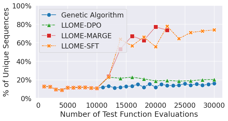
(a) Percent of sequences generated by each method that are unique.

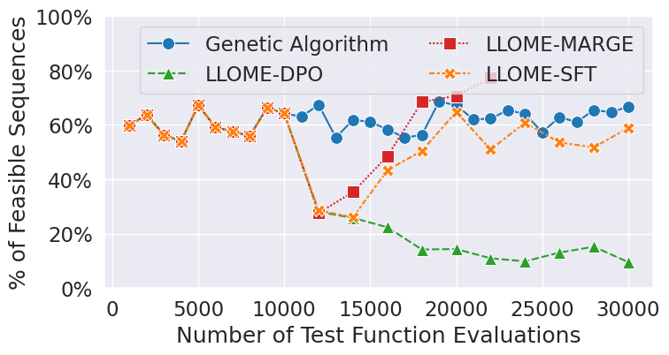
(b) Percent of unique sequences generated by each method that are also feasible.

Figure 3: The percentage of generated sequences that are unique or feasible. The lines for Llome-MargE end early because Llome-MargE discovers the optimal solution early.

Ehrlich Function Details

Unless stated otherwise, we evaluate Llome on an Ehrlich function with $L=32$, $|\mathcal{V}|=32$, $c=4$, and $k=q=4$.

LLMs generate sequences with low regret using few oracle labels.

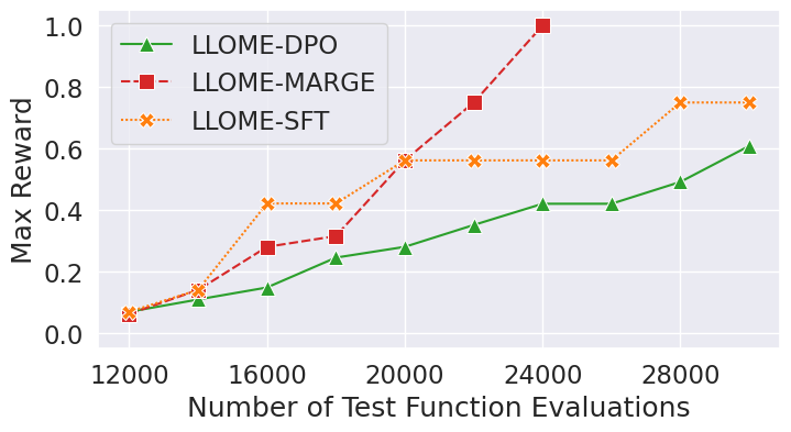
(a) Maximum reward achieved.

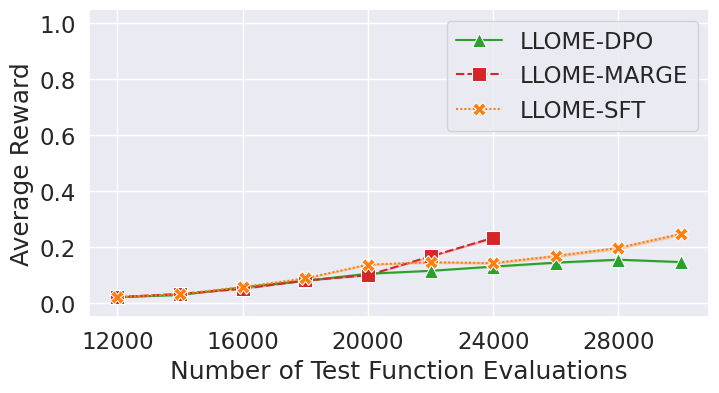
(b) Average reward.

Figure 11: Average and maximum reward achieved by methods that rely upon editing the original sequence. The shaded regions in (2(b)) represent the 95% confidence interval. The lines for Llome-MargE end early because Llome-MargE discovers the optimal solution early.

In Figure 2, we show both the average and minimum regret of Llome. While all three Llome variants achieve significantly lower minimum regret values than the genetic algorithm does, Llome-MargE is the only variant to discover the optimal solution and achieve a minimum regret of 0. However, the regret is based solely off the score of the output sequence (i.e. $\mathrm{regret}(x,y)=1-f(y)$ for $y\sim\pi_{\theta}(\cdot\mid x)$) and does not directly reflect how well the model improves the score of the input sequence. The reward, as given by Eq. 9, provides a more clear picture of the LLM’s ability to improve upon the input sequence. In Figure 11, we show the average and maximum reward achieved by each Llome variant. While all three variants achieve similar maximum reward throughout all iterations, Llome-SFT and Llome-MargE achieve significantly higher average reward than Llome-DPO.

SFT- and MargE-trained LLMs generate unique and feasible sequences, but DPO-trained LLMs struggle.

Successfully solving a highly-constrained optimization problem requires that the LLM be able to generate a diverse array of feasible sequences. Compared to the genetic algorithm, Figure 3(a) shows that all three Llome variants produce a higher percentage of unique sequences. However, Figure 3(b) indicates that Llome-SFT and LLOME-MargE often experience an initial dip in the percentage of feasible outputs before learning how to generate sequences in the feasible space. Llome-DPO, however, does not improve either the diversity or the feasibility of its outputs even when provided with more oracle labels. Like other past works [71; 81; 29; 72], we observe that the likelihood assigned by the DPO-trained LLM to both $y_{w}$ and $y_{l}$ continuously declines throughout training, implying that probability mass is moved to sequences outside of the training data distribution. Since the percentage of infeasible sequences generated by Llome-DPO increases over multiple iterations, it is likely that DPO moves some probability mass to infeasible regions of the sample space. As such, DPO may be ill-suited for training LLMs to adhere to strict constraints.

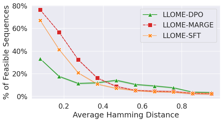
Figure 12: The percentage of feasible LLM-generated sequences, binned by the average Hamming distance (normalized by length) between the input and output. Shaded regions indicate the 95% confidence interval.

Although LLMs are capable of generating new feasible sequences, we also find that they suffer from the classic explore versus exploit tradeoff. When the LLM makes a larger edit to the input sequence, the output is less likely to be feasible (Fig. 12). For both Llome-SFT and Llome-MargE, an edit larger than 0.3 Hamming distance away from the input is less than 20% likely to be feasible. Since the $\Delta x$ threshold we set for the PropEn dataset formatting algorithm (Alg. 2) was 0.25, this is unsurprising. The LLM has never been trained on edits of larger than 0.25 Hamming distance. Overall, Llome-MargE exhibits the best tradeoff of all methods, producing the largest proportion of unique and feasible sequences for the smallest budget of test function evaluations (Fig. 3) and for moderately sized edits of Hamming distance $\leq 0.3$ (Fig. 12).

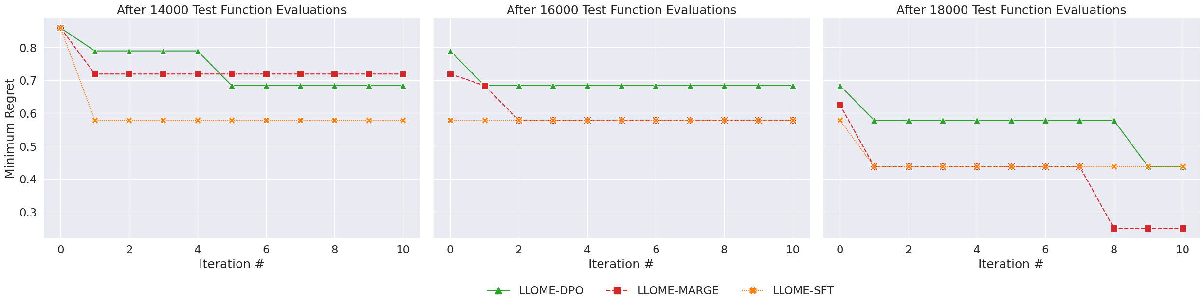
Figure 4: Minimum regret of sequences generated during the LLM inner loop, at each iteration of the iterative refinement process. The titles reflect the number of oracle labels that each LLM has been trained on. We defer the remaining plots for all other rounds of Llome to App. A.5, Fig. 13.

At inference time, LLMs can iteratively extrapolate beyond their training distributions.

Extrapolating beyond the training distribution is a well-known machine learning problem [10; 76; 50], especially without explicit guidance provided at inference time. Although some prior work has shown LLMs to be effective at iteratively generating sequences that monotonically increase a particular attribute to values beyond the training distribution [14; 70], much of this work focuses on simpler tasks such as increasing the positive sentiment of text or decreasing the $\Delta\Delta G$ of a well-studied protein. Since optimizing an Ehrlich function requires satisfying multiple constraints in addition to generating sequences that lie within a small feasible region, we posit that this evaluation is a more challenging assessment of LLMs’ inference-time extrapolation capabilities.

We display the iterative refinement results of Llome’s inner loop in Fig. 4, which suggest that LLMs iteratively produce edits that significantly reduce regret. However, the first few edits frequently improve the sequence whereas later edits are less likely to be helpful. This suggests that LLM’s inference-time extrapolative capabilities are limited – without further training or explicit guidance, LLMs may be unable to continuously improve a given sequence beyond a certain threshold. By alternating between optimizing the model’s parameters and optimizing the model’s outputs, we provide a sample-efficient method for iteratively bootstrapping the model’s extrapolative abilities using its own generations.

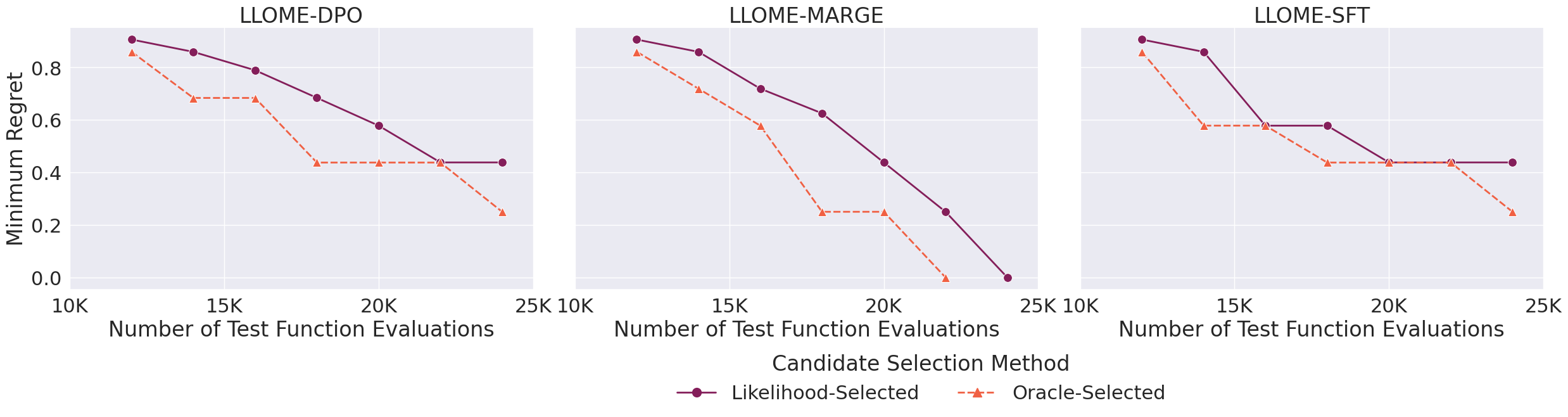
Figure 5: Minimum regret of candidates selected by either LLM likelihood or the oracle. Since the first 10K test function evaluations are seeds derived from the genetic algorithm, we show only candidates generated after the first 10K.

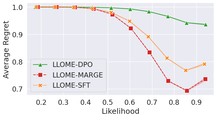
(a) Model likelihood vs. regret of generations.

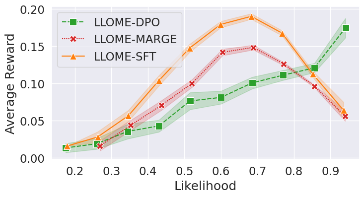
(b) Model likelihood vs. reward of generations.

Figure 6: Calibration curves comparing likelihood versus the average regret (6(a)) and reward (6(b)) of each method’s generated sequences. Shaded regions represent the mean $\pm$ two standard errors.

LLMs are moderately effective at ranking their own outputs.

The iterative refinement process requires that the LLM rank and filter its own outputs (Alg. 4), but we have not yet considered how effective the LLM is at selecting the best candidates. When compared to oracle selection (i.e. using the ground-truth Ehrlich score to select candidates), we find that the likelihood method often selects high-scoring candidates, but not necessarily the highest scoring ones (Fig. 5). To better understand this gap between likelihood selection and oracle selection, we examine the calibration curves of average likelihood versus regret and reward on Llome-generated sequences in Fig. 6. Although it appears that Llome-DPO is the only variant to exhibit a calibration curve that monotonically decreases and increases with regret and reward, respectively, Llome-DPO also produces the fewest sequences with regret outside of the training distribution. Calibration becomes more difficult when evaluated on more sequences outside the training distribution, as is the case for Llome-MargE and Llome-SFT. While SFT- and MargE-trained LLMs generally assign higher likelihood to lower-regret sequences than DPO-trained LLMs (Fig. 6(a)), they also exhibit some degree of overconfidence. Indeed, we observe that the likelihood and reward of SFT- and MargE-generated sequences appear to be inversely correlated for likelihoods exceeding 0.7 (Fig. 6(b)). Since these higher-likelihood sequences also correspond to the lowest regret values (Fig. 6(a)), we hypothesize that LLMs may become increasingly miscalibrated as their outputs extend beyond the training distribution.

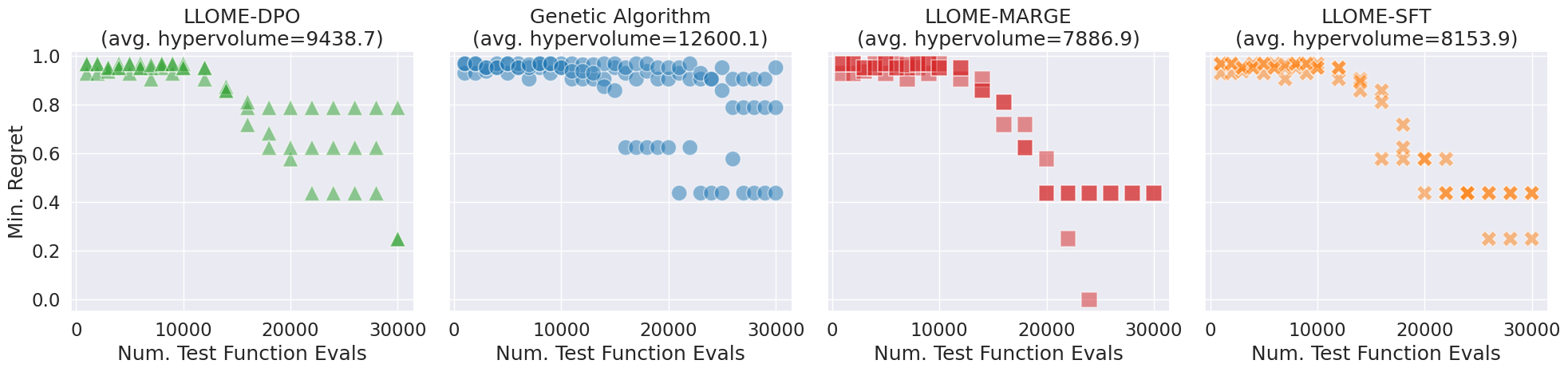
Figure 7: Pareto frontiers of evaluation budget vs. minimum regret for a variety of Llome hyperparameter settings, Ehrlich functions, and seed datasets. The average hypervolume refers to the average $(\text{number of test function evaluations}\times\text{minimum regret})$. Lower hypervolume is better.

How sensitive is Llome to hyperparameters, test function difficulty, and seed dataset?

An important aspect of an optimization algorithm is how robust it is to hyperparameter settings, problem difficulty, and choice of seed examples. To explore the robustness of Llome, we evaluate Llome on two different Ehrlich functions, two seed datasets (generated by two instances of the genetic algorithm with different $p_{m}$ values), and varying budgets of test function evaluations. The Ehrlich functions $f_{1}$ and $f_{2}$ have parameters $L=32,|\mathcal{V}|=32,c=k=q=4$ and $L=16,|\mathcal{V}|=32,c=k=q=4$. The genetic algorithms have $p_{m}=0.005$ and $p_{m}=0.01$, and the budget of test function evaluations varies from 1K to 30K. We present the Pareto frontiers and corresponding hypervolumes of these experiments in Fig. 7. While all three Llome variants exhibit significantly lower average hypervolume than the genetic algorithm, Llome-MargE is the most sample efficient.

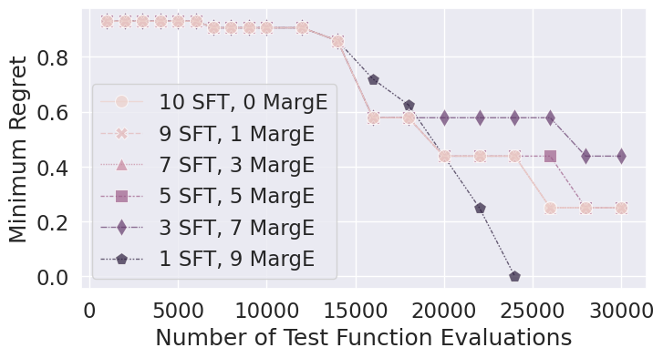
(a) Minimum regret for multi-stage SFT+MargE training.

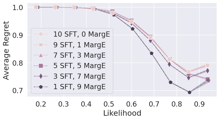
(b) Calibration curve of likelihood vs. regret for multi-stage SFT+MargE training.

Figure 8: Minimum regret and calibration curves for multi-stage LLM training.

When is explicit reward information required during training?

Since we have observed that Llome-SFT and Llome-MargE perform similarly up to the point of 20K test function evaluations (Fig. 2(a)), we might hypothesize that incorporating explicit reward values into the training objective is only necessary once the LLM is closer to the optimum. Since MargE requires a larger memory footprint than SFT (due to the need to store and compute likelihoods with both $\pi_{\theta}$ and $\pi_{\text{Ref}}$), training the LLM with further rounds of SFT before switching to MargE would be more efficient than relying mostly on MargE training. We test this hypothesis via a multi-stage pipeline, where early rounds of Llome use SFT training, and later rounds use MargE. We keep the total number of LLM training rounds constant at 10 (unless the LLM finds the optimal solution earlier) and vary the proportion of rounds that use SFT versus MargE, as shown in Fig. 8. We refer to the pipeline with $i$ rounds of SFT training followed by $j$ rounds of MargE training as Llome-SFT_i-MargE_j. We find that Llome-SFT₁-MargE₉ not only is the sole pipeline to find the optimal solution (Fig. 8(a)), but also achieves the best calibration curve (Fig. 8(b)). In contrast, switching from SFT to MargE training at an intermediate point results in the worst performance. It appears that SFT and MargE may have conflicting loss landscapes – if we first train for a few rounds with the SFT loss, subsequently switching to MargE training impedes the LLM’s progress. We additionally explore in App. A.5 the effects of incorporating the reward in different ways during training.

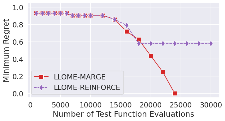
Figure 9: Minimum regret achieved by Llome-MargE and Llome-REINFORCE.

Does fulfilling the Strong Interpolation Criteria (SIC) matter for LLM training?

We previously proposed a new LLM training objective, MargE, for the purposes of easily incorporating reward information while fulfilling SIC [39]. However, there also exist policy gradient methods such as REINFORCE [104] that directly optimize for maximal reward without the steep complexity of RLHF [94; 116]. Although these policy gradient methods do not fulfill SIC, they have been shown to perform comparably to RLHF [94; 116] and RL-free variants such as DPO [79] and RAFT [26]. The primary difference between MargE and a policy gradient method like REINFORCE, then, is that MargE attempts to smoothly interpolate between $\pi^{*}$ and $\pi_{\text{Ref}}$, whereas the KL-regularized REINFORCE algorithm interpolates between $\pi^{\delta}$ (the degenerate reward-maximizing distribution) and $\pi_{\text{Ref}}$. To test whether this difference has a meaningful impact on an LLM’s optimization capabilities, we compare Llome-MargE with Llome-REINFORCE, where we use a KL-regularized version of REINFORCE with the same importance sampling and self-normalization techniques as in MargE:

$$\mathcal{L}_{\text{REINFORCE}}(\pi_{\theta},\pi_{\text{Ref}};\mathbb{D}_{x})=\underset{\begin{subarray}{c}x\sim\mathbb{D}_{x},\\ y\sim\pi_{\text{Ref}}(\cdot\mid x)\end{subarray}}{\mathbb{E}}\left[-\frac{\pi_{\theta}(y|x)}{\pi_{\text{Ref}}(y|x)}r(x,y)\log\pi_{\theta}(y|x)-\lambda\frac{\log\pi_{\theta}(y|x)}{|y|}\right]$$ (10)

The implications of this objective are intuitive – greater weight is placed on the loss for higher reward examples, and vice versa. However, in the limit of $\lambda\to 0$, we have $\pi_{\theta_{\text{REINFORCE}}^{*}}=\arg\max_{\pi_{\theta}}\mathbb{E}_{y\sim\pi_{\theta}(\cdot|x)}r(x,y)/\pi_{\text{Ref}}(y|x)$, which is a degenerate distribution that places all probability mass on $(x^{\prime},y^{\prime})\in\operatorname*{arg\,max}_{(x,y)}r(x,y)/\pi_{\text{Ref}}(y|x)$, thereby violating SIC. By inspecting Fig. 9, we observe that although Llome-REINFORCE does decrease the regret to some degree, it plateaus early and does not reach optimality.

5.1 Related Work

Our work combines insights from multiple areas of research, including discrete sequence black-box optimization, controllable text generation, and LLMs for optimization and scientific discovery.

Discrete Sequence Black-Box Optimization

Many algorithms for discrete sequence optimization take inspiration from directed evolution [6], a combination of random mutagenesis (a means to generate variants of the current solution) and high throughput screening (discriminative selection pressure). Researchers have explored many types of variant generators, including random mutagenesis [7; 89], reinforcement learning [4], denoising with explicit discriminative guidance [92; 58; 32], and denoising with implicit discriminative guidance [96]. While these algorithms are all very general in principle, in practice a substantial amount of effort is required to actually implement these algorithms for new problems due to changes in the problem setup. In this work we investigate whether LLMs offer a path to a solution that can rapidly be applied to new problems with minimal engineering effort.

LLMs for Optimization and Scientific Discovery

Much of the work on LLMs for optimization has been inspired by the design of classic black-box optimizers (BBO) such as evolutionary algorithms, bayesian optimizers, and random search methods. BBOs are characterized by a lack of information about the true objective function. Instead, only inputs and their corresponding objective values are provided to the optimizer, with no gradient or priors about the objective. Since these optimization problems are often expressible in formal mathematical, logical, or symbolic terms, many initial attempts at LLMs for optimization used the LLMs to first translate a natural language description of the problem into code or a modeling language, prior to passing this formalization into an auxiliary solver [83; 2; 61; 1]. This approach was often quite effective, as it utilized the wealth of past work on LLMs for named entity recognition [3; 99; 102; 105; 5, ; NER], semantic parsing [27; 36; 87; 86; 85; 88; 18; 93], and code generation [17; 66; 65; 110; 75]. The NL4OPT competition [83], for example, decomposed LLMs-for-BBO into two subtasks: (1) the translation of a natural language description into a graph of entities and relations between the entities, and (2) a formalization of the optimization problem into a canonical logical reperesentation that could be solved by many commercial solvers. Winning approaches often employed ensemble learning [37; 101; 67; 25], adversarial learning [101; 67], and careful data pre-/post-processing and augmentation [37; 67; 41]. Later work demonstrated that pre-trained LLMs like GPT-4 could achieve competitive performance on NLP4OPT without the NER stage [2], though the F1 score still trailed behind the state-of-the-art translation+NER approaches from the winning NL4OPT entries. Outside of NL4OPT, Gao et al. [30], He-Yueya et al. [38], AhmadiTeshnizi et al. [1], and Mittal et al. [61] use an LLM to formalize math, mixed integer linear programming, and combinatorial reasoning problems from a natural language description before offloading the solving to a Python interpreter or symbolic solver. Each work notes that the LLM performs better in this decomposed framework than through prompting alone.

Yet other approaches tackle LLMs-for-optimization directly with the LLM, without additional solvers. As Song et al. [91] argues, LLMs offer both powerful in-context learning abilities and a flexible natural-language interface capable of expressing a wide variety of problems. Many techniques embed the LLM in an evolutionary algorithm, using the LLM as a mutation or crossover operator [15; 34; 60; 49; 63; 52; 48; 53; 84]. In this setting, the LLM provides a diversity of samples while the evolutionary algorithm guides the search towards high-fitness regions. This strategy is a form of bi-level optimization, in which two nested optimization problems (one nested within the other) are solved in alternation. It is common for the outer loop to optimize the model’s parameters, and for the inner loop to optimize the model’s outputs [20; 35]. Ma et al. [54] combine this approach with feedback from physical simulations in the inner optimization loop to enable LLMs to complete various scientific optimization tasks, such as constitutive law discovery and designing molecules with specific quantum mechanical properties. Although their use of an LLM in a bi-level optimization loop is similar to ours, they directly train their parameters using differentiable simulations whereas we do not assume access to the gradients of the ground truth rewards. Our work additionally explores various aspects of LLM training that allow the LLM to improve its optimization abilities despite not having access to ground-truth rewards in the inner loop. Lastly, other approaches avoid gradient optimization altogether and focus purely on prompt-based optimization, demonstrating success on diverse tasks such as hill-climbing [33], Newton’s method [64], hyperparameter search [108], and prompt engineering [44; 77; 106].

Controllable Text Generation

Controllable text generation (CTG) is a special case of optimization. Rather than searching for sequences that maximize the objective function, the goal is to produce a sequence with a particular attribute value (e.g. having a certain number of words, a more positive sentiment than the input, or a particular biological motif). In some aspects, this may be an easier task – the optimizer need not generate an optimal sequence that is likely outside the distribution of its training data. In others, this may also be more difficult. Targeting particular attribute values requires precision and fine-grained knowledge of the shape of the entire objective function, rather than only the neighborhood of the optima. Although LLM prompting is in itself considered a form of CTG [78; 11], prompting alone tends to offer better control for more open-ended, higher level instructions (e.g. “write a story in the style of Shakespeare”) than for fine-grained constraints (e.g. “rewrite this sentence using only 10 words”) [12].

One common approach is to use control codes, or unique strings pre-pended in front of a training example that indicates which attribute is represented in the example’s target [43; 70; 82; 56]. This approach is typically less generalizable to new attributes or instructions, due to the need to re-train the model. However, more recent work has shown that LLMs are capable of learning to use these control codes in-context [113; 115], simplifying the process by which new attributes can be introduced. A popular alternative technique is inference-time guidance, which uses auxiliary tools [73] or models [22; 51; 24; 23] to guide the LLM decoding process.

6 Conclusions

Our work is a response to the lack of both non-trivial synthetic benchmarks for biophysical sequence optimizers and rigorous analyses of how LLMs perform on these highly-constrained optimization tasks in realistic settings. Our proposed test functions bear significant geometric similarities to real biophysical sequence optimization tasks and allow for rapid iteration cycles. In addition, although a wealth of work exists that adapts LLMs for biophysical tasks, few have studied the abilities of LLMs to adhere to hard constraints in realistic bi-level optimization settings. To that end, we propose and analyze Llome, a framework for incorporating LLMs in bilevel optimization algorithms for highly constrained discrete sequence optimization problems. We show that Llome discovers lower-regret solutions than a genetic algorithm, even with very few test function evaluations. When combined with MargE training, Llome is significantly more sample efficient than Llome-SFT or Llome-DPO, demonstrating its potential to be useful in data-sparse lab settings. Our findings also highlight that LLMs can robustly extrapolate beyond their training data, but are occasionally miscalibrated and benefit from training with ground truth rewards.

7 Acknowledgements

We thank Natasa Tagasovska and the Prescient Design LLM team for valuable discussions and feedback during the development of this project. The authors acknowledge the Prescient Design Engineering team for providing HPC and consultation resources that contributed to the research results reported within this paper.

Appendix A Appendix

A.1 Ehrlich Functions

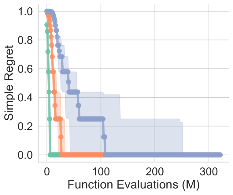
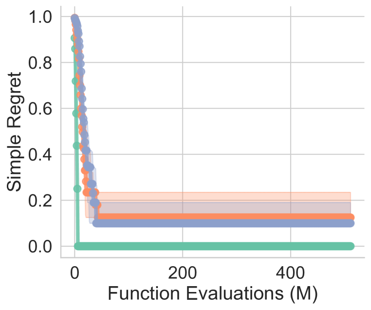
Figure 10: Here we show how the difficulty of the test problem can be controlled by varying Ehrlich function parameters, keeping the optimizer fixed to the robust GA baseline defined in Sec. A.3.3. Starting from a fixed set of reference parameters we vary each parameter individually. For this optimizer, the problem difficulty depends most strongly on the quantization parameter $q$. The x-axis is defined in millions (M) of Ehrlich function evaluations, demonstrating the difficulty of these Ehrlich functions, even for a small number of short motifs.

One major advantage of procedurally generating specific instances of Ehrlich functions is we can generate as many distinct instances of this test problem as we like. In fact it creates the possibility of “train” functions for algorithm development and hyperparameter tuning and “test” functions for evaluation simply by varying the random seed. These functions can also be defined with arbitrary levels of difficulty, as shown in Fig. 10. However, defining a random instance that is nevertheless provably solvable takes some care in the problem setup, which we now explain.

A.1.1 Constructing the Transition Matrix

Here we describe an algorithm to procedurally generate random ergodic transition matrices $A$ with infeasible transitions. A finite Markov chain is ergodic if it is aperiodic and irreducible (since every irreducible finite Markov chain is positive recurrent). Irreducibility means every state can be reached with non-zero probability from every other state by some sequence of transitions with non-zero probability. We will ensure aperiodicity and irreducibility by requiring the zero entries of $A$ to have a banded structure. For intuition, consider the transition matrix

$$\begin{bmatrix}0.4&0.3&0&0.3\\ 0.3&0.4&0.3&0\\ 0&0.3&0.4&0.3\\ 0.3&0&0.3&0.4\end{bmatrix}$$

Recalling that $v$ is the number of states, we can see that every state $x$ communicates with every other state $x^{\prime}$ by the sequence $x\rightarrow(x+1)\mod v\rightarrow\dots\rightarrow(x^{\prime}-1)\mod v\rightarrow x^{\prime}$. We also see that the chain is aperiodic since every state $x$ has a non-zero chance of being repeated.

To make things a little more interesting we will shuffle (i.e. permute) the rows of a banded structured matrix (with bands that wrap around), but ensure that the diagonal entries are still non-zero. Note that permuting the bands does not break irreducibility because valid paths between states can be found by applying the same permutation action on valid paths from the unpermuted matrix. We will also choose the non-zero values randomly, using the shuffled banded matrix only as a binary mask $B$ as follows:

$$\overset{\text{(banded matrix)}}{\begin{bmatrix}1&1&0&1\\ 1&1&1&0\\ 0&1&1&1\\ 1&0&1&1\end{bmatrix}} \xrightarrow[\text{shuffle}]{}\begin{bmatrix}1&0&1&1\\ 1&1&1&0\\ 1&1&0&1\\ 0&1&1&1\end{bmatrix},$$

$$\xrightarrow[\text{diag}=1]{}\begin{bmatrix}1&0&1&1\\ 1&1&1&0\\ 1&1&1&1\\ 0&1&1&1\end{bmatrix}$$

$$=B.$$

Now we draw the transition matrix starting with a random matrix with IID random normal entries, softmaxing with temperature $\tau>0$ to make the rows sum to 1, applying the mask $B$, and renormalizing the rows by dividing by the sum of the columns after masking.

$$Z =\overset{\text{(randn matrix)}}{\begin{bmatrix}+1.41&+1.67&-1.52&+0.63\\ -0.35&+0.45&+0.86&-0.49\\ +1.42&-1.31&-0.31&+1.43\\ -0.02&+1.55&-0.26&+1.13\end{bmatrix},}$$

$$\xrightarrow[\text{softmax}]{}\begin{bmatrix}0.36&0.46&0.02&0.16\\ 0.13&0.30&0.45&0.12\\ 0.44&0.03&0.08&0.45\\ 0.10&0.49&0.08&0.33\end{bmatrix},$$

$$\xrightarrow[\odot B]{}\begin{bmatrix}0.36&0&0.02&0.16\\ 0.13&0.30&0.45&0\\ 0.44&0.03&0.08&0.45\\ 0&0.49&0.08&0.33\end{bmatrix},$$

$$\xrightarrow[\text{norm}]{}\begin{bmatrix}0.66&0&0.04&0.30\\ 0.15&0.34&0.51&0\\ 0.44&0.03&0.08&0.45\\ 0&0.55&0.09&0.36\end{bmatrix}=A.$$

We can also verify that $A$ is ergodic numerically by checking the Perron-Frobenius condition,

$$(A^{m})_{ij}>0,\;\forall i,j,$$ (11)

where $m=(v-1)^{2}+1$, $A^{1}=A$, and $A^{b}=AA^{b-1}$ for all $b>1$. In our example, if $v=4$ then $m=10$ and we verify on a computer that

$$A^{10}=\begin{bmatrix}0.33&0.23&0.17&0.27\\ 0.33&0.23&0.17&0.27\\ 0.33&0.23&0.17&0.27\\ 0.33&0.23&0.17&0.27\\ \end{bmatrix}$$

A.1.2 Constructing Jointly Satisfiable Spaced Motifs

Here we describe how to procedurally generate $c$ spaced motifs of length $k$ such that the existence of a optimal solution $\mathbf{x}^{*}$ with length $L$ with non-zero probability under a transition matrix $A$ generated by the procedure in Appendix A.1.1 can be verified by construction. If we simply sampled motifs completely at random from $\mathcal{V}^{k}$ we cannot be sure that a solution attaining a global optimal value of 1 is actually feasible under the DMP constraint.

First we require that $L\geq c\times k$. Next to define the motifs, we draw a single sequence of length $c\times k$ from the DMP defined by $A$ (the first element can be chosen arbitrarily). Then we chunk the sequence into $c$ segments of length $k$, which defines the motif elements $\mathbf{m}^{(i)}$. This ensures that any motif elements immediately next to each other are feasible, and ensures that one motif can transition to the next if they are placed side by side.

Next we draw random offset vectors $\mathbf{s}^{(i)}$. The intuition here is we want to ensure that an optimal solution can be constructed by placing the spaced motifs end-to-end. If we fix $c\times k$ positions to satisfy the motifs, there are $L-c\times k$ “slack” positions that we evenly distribute (in expectation) between the spaces between the elements of each motif. We set the first element of every spacing vector $s^{(i)}_{1}$ to 0, then set the remaining elements to the partial sums of a random draw from a discrete simplex as follows:

$$\mathbf{w}^{(i)} \sim\mathcal{U}\left(\{\mathbf{w}\in\mathbb{R}^{k-1}\mid\sum w_{i}=1\}\right).$$ (12)

$$s^{(i)}_{j+1} =s^{(i)}_{j}+1+\lfloor w^{(i)}_{j}\times(L-c\times k)//c\rfloor.$$ (13)

Finally, recall that in Appendix A.1.1 we ensured that self-transitions $x\rightarrow x$ always have non-zero probability. This fact allows us to construct a feasible solution that attains the optimal value by filling in the spaces in the motifs with the previous motif elements.

As a concrete example, suppose $L=8$, $c=2$, and $k=2$ (hence $s_{\max}=3$) and we draw the following set of spaced motifs:

$$\begin{bmatrix}0&3&1&2\end{bmatrix} \rightarrow\begin{bmatrix}0&3\\ 1&2\end{bmatrix}=\begin{bmatrix}\mathbf{m}^{(1)}\\ \mathbf{m}^{(2)}\end{bmatrix},$$ (14)

$$\begin{bmatrix}\mathbf{s}^{(1)}\\ \mathbf{s}^{(2)}\end{bmatrix} =\begin{bmatrix}0&3\\ 0&3\end{bmatrix}.$$ (15)

An optimal solution can then be constructed as follows:

$$\mathbf{x}^{*}=\begin{bmatrix}0&0&0&3&1&1&1&2\\ \end{bmatrix}$$

Note that this solution is only used to verify that the problem can be solved. In practice solutions found by optimizers like a genetic algorithm will look different. Additionally if $L\gg c\times k$ then the spaced motifs can often be feasibly interleaved without clashes.

A.1.3 Defining The Initial Solution

Optimizer performance is generally quite sensitive to the choice of initial solution. In our experiments we fixed the initial solution to a single sequence of length $L$ drawn from the DMP.

A.2 Derivations

Derivation of the MargE Objective

To derive a training objective that fulfills SIC, we follow Hu et al. [39] and propose an objective that takes the following general form:

$$\arg\min_{\theta}\left[\mathbb{KL}(\tilde{\pi}_{\theta}\|\pi^{*})+\lambda\mathbb{KL}(\pi_{\text{Ref}}\|\tilde{\pi}_{\theta})\right]$$ (17)

where $\pi^{*}$ is the target reward distribution and $\tilde{\pi}_{\theta}$ is the length-normalized version of $\pi_{\theta}$.

Since past work has indicated that preference-tuned models often spuriously favor longer generations, we follow Malladi [57]; Meng et al. [59] by instead using length-normalized likelihoods. Additionally, it is standard in past literature [116; 46] to model $\pi^{*}$ as a Boltzmann function of the reward. That is,

$$\pi^{*}(y\mid x)=\frac{1}{Z(x)}\exp(r(x,y))$$

where $Z(x)$ is the partition function. Although this partition function is not guaranteed to converge due to the observation that LLMs often place non-zero probability mass on infinite-length sequences [28; 103], we make the assumption for now that this effect is negligible. This results in a formulation of the optimal policy that is Bradley-Terry with respect to the rewards. I.e.,

$$\log\pi^{*}(y_{1}|x)-\log\pi^{*}(y_{2}|x)=r(x,y_{1})-r(x,y_{2})$$

Then, the first term of Equation 17 can be expanded as:

$$\arg\min_{\theta}\mathbb{KL}(\tilde{\pi}_{\theta}\|\pi^{*})=\arg\min_{\theta}\underset{\begin{subarray}{c}x\sim\mathbb{D}_{x},\\ y\sim\tilde{\pi}_{\theta}(\cdot\mid x)\end{subarray}}{\mathbb{E}}\log\left(\frac{\tilde{\pi}_{\theta}(y|x)}{\pi^{*}(y|x)}\right)$$

Since we cannot directly sample from $\tilde{\pi}_{\theta}$, we approximate it by sampling from the un-normalized policy:

$$\approx\arg\min_{\theta}\underset{\begin{subarray}{c}x\sim\mathbb{D}_{x},\\ y\sim\pi_{\theta}(\cdot\mid x)\end{subarray}}{\mathbb{E}}\left[\frac{\log\pi_{\theta}(y|x)}{|y|}-r(x,y)+\log Z(x)\right]$$

$$=\arg\min_{\theta}\underset{\begin{subarray}{c}x\sim\mathbb{D}_{x},\\ y\sim\pi_{\theta}(\cdot\mid x)\end{subarray}}{\mathbb{E}}\left[\frac{\log\pi_{\theta}(y|x)}{|y|}-r(x,y)\right]$$

Rather than re-sampling from $\pi_{\theta}$ after every step of training, we approximate this step using importance sampling:

$$\mathbb{KL}(\pi_{\theta}\|\pi^{*}) \approx\underset{\begin{subarray}{c}x\sim\mathbb{D}_{x},\\ y\sim\pi_{\theta}(\cdot\mid x)\end{subarray}}{\sum}\frac{\pi_{\theta}(y|x)}{\pi_{\text{Ref}}(y|x)}\pi_{\text{Ref}}(y|x)\left[\frac{\log\pi_{\theta}(y|x)}{|y|}-r(x,y)\right]$$

$$\approx\underset{\begin{subarray}{c}x\sim\mathbb{D}_{x},\\ y\sim\pi_{\text{Ref}}(\cdot\mid x)\end{subarray}}{\mathbb{E}}\frac{\pi_{\theta}(y|x)}{\pi_{\text{Ref}}(y|x)}\left[\frac{\log\pi_{\theta}(y|x)}{|y|}-r(x,y)\right]$$ (18)

For the second term of Equation 17, we remove terms not depending on $\theta$, resulting in the standard token-averaged cross-entropy loss:

$$\min_{\theta}\mathbb{KL}(\pi_{\text{Ref}}\|\tilde{\pi}_{\theta})\equiv\min_{\theta}\underset{\begin{subarray}{c}x\sim\mathbb{D}_{x},\\ y\sim\pi_{\text{Ref}}(\cdot\mid x)\end{subarray}}{\mathbb{E}}-\frac{\log\pi_{\theta}(y|x)}{|y|}$$ (19)

Plugging Equations 18 and 19 back into 17, we obtain

$$\mathcal{L}_{\text{MargE}}(\pi_{\theta},\pi_{\text{Ref}};\mathbb{D}_{x})=\underset{\begin{subarray}{c}x\sim\mathbb{D}_{x},\\ y\sim\pi_{\text{Ref}}(\cdot\mid x)\end{subarray}}{\mathbb{E}}\left[\frac{\pi_{\theta}(y|x)}{\pi_{\text{Ref}}(y|x)}\left(\frac{\log\pi_{\theta}(y|x)}{|y|}-r(x,y)\right)-\lambda\frac{\log\pi_{\theta}(y|x)}{|y|}\right].$$

Since importance sampling often leads to high variance of the gradient estimates in practice [68], we instead use the self-normalized version of this objective (Eq. 32).

Lemma 1.

Given a Bradley-Terry model $\pi(y|x)=\frac{1}{Z(x)}\exp(r(x,y))$ with partition function $Z(x)$, if reward function $r(x,y)=f(y)-f(x)$ for some real-valued scoring function $f(x):\mathcal{V}^{*}\to\mathbb{R}$, then $\pi(y|x)=\pi(y|z)$ for any pair $x,z\in\mathrm{dom}(f)$.

Proof.

Since $Z(x)$ is the normalizing constant for $\pi(y|x)$, we can write

$$Z(x) =\sum_{y^{\prime}\in\mathcal{V}^{*}}\exp(r(x,y^{\prime}))$$ (20)

$$=\sum_{y^{\prime}\in\mathcal{V}^{*}}\exp(f(y^{\prime})-f(x))$$ (21)

$$=\frac{1}{\exp(f(x))}\sum_{y^{\prime}\in\mathcal{V}^{*}}\exp(f(y^{\prime})).$$ (22)

It follows that

$$\pi(y|x) =\frac{\exp(f(x))}{\sum_{y^{\prime}\in\mathcal{V}^{*}}\exp(f(y^{\prime}))}\exp(r(x,y))$$ (23)

$$=\frac{\exp(f(x)+f(y)-f(x))}{\sum_{y^{\prime}\in\mathcal{V}^{*}}\exp(f(y^{\prime}))}$$ (24)

$$=\frac{\exp(f(y))}{\sum_{y^{\prime}\in\mathcal{V}^{*}}\exp(f(y^{\prime}))}$$ (25)

$$=\frac{\exp(f(y)+f(z)-f(z))}{\sum_{y^{\prime}\in\mathcal{V}^{*}}\exp(f(y^{\prime}))}$$ (26)

$$=\frac{\exp(f(z))\exp(r(z,y))}{\sum_{y^{\prime}\in\mathcal{V}^{*}}\exp(f(y^{\prime}))}$$ (27)

$$=\frac{1}{Z(y)}\exp(r(z,y))$$ (28)

$$=\pi(y|z)$$ (29)

∎

A.3 Algorithms

Input: Scoring function $f$; pretrained LLM $\pi_{\theta_{0}}$ parameterized by initial weights $\theta_{0}$; initial seed sequence $\mathbf{x}_{0}\in\mathcal{F}$; $k$ number of test function evaluations per round; $T$ number of Llome rounds.

1 $S\leftarrow\{(\mathbf{x}_{0},f(\mathbf{x}_{0}))\}$;

$\mathcal{X}_{0}\leftarrow\textsc{GeneticAlgorithm}(\mathbf{x}_{0},n_{0})$ ;

  /* Seed with $n_{0}$ rounds of evolution. */

$S_{0}\leftarrow\{(\mathbf{x},f(\mathbf{x}))\mid\mathbf{x}\in\mathcal{X}_{0}\}$ ;

  /* Score the initial candidates. */

2 $S\leftarrow S\cup S_{0}$;

3 $i\leftarrow 0$;

while $i<T$ ;

  /* Outer Loop */

4 do

5       $\mathcal{D}_{i}\leftarrow\textsc{DatasetFormatting}(S_{i})$;

6       $\theta_{i+1}\leftarrow\textsc{Train}(\theta_{i},\mathcal{D}_{i})$;

       $\mathcal{X}_{i+1}\leftarrow\textsc{IterativeRefinement}(\pi_{\theta_{i+1}},S_{i})$ ;

        /* Inner Loop */

       $\mathcal{X}_{i+1}\leftarrow\textsc{Filter}(\mathcal{X}_{i+1},k)$;

        /* Filter $\mathcal{X}_{i+1}$ down to $k$ samples. */

       $S_{i+1}\leftarrow\{(\mathbf{x},f(\mathbf{x}))\mid\mathbf{x}\in\mathcal{X}_{i+1}\}$ ;

        /* Oracle labeling. */

7       $S\leftarrow S\cup S_{i+1}$;

8       $i\leftarrow i+1$;

9      

10 end while

Output: $\arg\max_{(\mathbf{x},f(\mathbf{x}))\in S}f(\mathbf{x})$

Algorithm 1 Llome, an approach for bilevel optimization of highly constrained sequence optimization problems with LLMs. We use $n_{0}=10$, $k=2000$, and $T=10$.

Input: Dataset $S=\{(\mathbf{x},y)\}$ of particles $\mathbf{x}$ and scores $y$; $k_{n}$ number of nearest neighbors to find; distance function $d$; threshold $\Delta x$; dataset type $type=(\text{``binary"}\mid\text{``triple"})$

1

2if $type=\text{``binary"}$ then

3       $\mathcal{D}\leftarrow\left\{(x_{i},x_{j})\bigg{\lvert}\,\begin{subarray}{c}(x_{i},y_{i}),(x_{j},y_{j})\in S\\ x_{j}\in\textsc{KNearestNeighbors}(x_{i},k_{n})\\ d(x_{i},x_{j})\leq\Delta_{x}\\ f(x_{j})>f(x_{i})\end{subarray}\right\}$;

4      

5else

6       $\mathcal{D}\leftarrow\left\{(x_{i},x_{j},x_{k})\bigg{\lvert}\,\begin{subarray}{c}(x_{i},y_{i}),(x_{j},y_{j}),(x_{k},y_{k})\in S\\ x_{j},x_{k}\in\textsc{KNearestNeighbors}(x_{i},k_{n})\\ d(x_{i},x_{j})\leq\Delta_{x},d(x_{i},x_{k})\leq\Delta_{x}\\ f(x_{j})>f(x_{i}),f(x_{i})\geq f(x_{k})\end{subarray}\right\}$

7 end if

Output: $\mathcal{D}$

Algorithm 2 $\textsc{DatasetFormatting}(S)$. An algorithm that adapts PropEn [96] to create pairs or triples of data for LLM training. We use $k_{n}=30$, $\Delta x=0.25$, and the fractional Hamming distance as $d$.

Input: Pretrained LLM $\pi_{\theta}$; dataset $S=\{(\mathbf{x},y)\}$ of sequences $\mathbf{x}$ and scores $y$; $n_{s}$ number of seed examples; $n_{i}$ rounds of iteration per example; $n_{o}$ outputs per iteration; $T$ set of temperatures to sample with.

1 $S^{\prime}\leftarrow\{\}$;

$\mathcal{X}\leftarrow\{\mathbf{x}\mid(\mathbf{x},y)\in\textsc{TopK}(S,n_{s})\}$;

  /* Obtain $n_{s}$ seed examples from the top training examples by score. */

2 for $\mathbf{x}\in\mathcal{X}$ do

3       $\mathbf{x}_{0}\leftarrow\mathbf{x}$;

4       $i\leftarrow 0$;

5       for $i<n_{i}$ do

6             $\mathbf{x}_{i+1}\leftarrow\textsc{GreedyDecoding}(\pi_{\theta};\mathbf{x}_{i})$;

7             $S^{\prime}\leftarrow S^{\prime}\cup\{\mathbf{x}_{i+1}\}$;

8             $i\leftarrow i+1$;

9            

10       end for

11      for $t\in T$ do

12             $i\leftarrow 0$;

13             for $i<n_{i}$ do

                   $\mathcal{X}_{i}\leftarrow\{\mathbf{x}_{j}\sim\pi_{\theta}^{t}(\cdot\mid\mathbf{x}_{i})\}_{j=1}^{n_{o}}$;

                    /* Sample $n_{o}$ sequences using temperature $t$. */

14                   $S^{\prime}\leftarrow S^{\prime}\cup\mathcal{X}_{i}$;

                   $\mathbf{x}_{i+1}\leftarrow\arg\max_{\mathbf{x}^{\prime}\in\mathcal{X}_{i}}\pi_{\theta}(\mathbf{x}^{\prime}\mid\mathbf{x})$;

                    /* Select the highest-likelihood sample as the input for the next iteration. */

15                   $i\leftarrow i+1$;

16                  

17             end for

18            

19       end for

20      

21 end for

22$S^{\prime}\leftarrow\textsc{Deduplicate}(S^{\prime})$;

Output: $S^{\prime}$

Algorithm 3 $\textsc{IterativeRefinement}(\pi_{\theta};S)$. $\pi_{\theta}^{t}$ represents $\pi_{\theta}$ with temperature $t$ scaling. We use $n_{s}=200$, $n_{i}=10$, $n_{o}=10$, and $T=[0.6,0.8,1.0,1.2,1.4,1.6]$.

Input: LLM $\pi_{\theta}$ that generated the sequences; dataset $\mathcal{X}=\{(\mathbf{x},y)\}$ of sequences $\mathbf{x}$ and scores $y$; likelihood threshold $p_{\text{min}}$; maximum proportion of infeasible sequences $p_{\text{max-infeas}}$; final output size $k$.

$\mathcal{X}\leftarrow\{((\mathbf{x},y),\pi_{\theta}(\mathbf{x}))\mid(\mathbf{x},y)\in\mathcal{X}\}$;

  /* Compute likelihoods. */

1 $\mathcal{X}\leftarrow\{(\mathbf{x},y)\mid\pi_{\theta}(\mathbf{x})>p_{\text{min}},((\mathbf{x},y),\pi_{\theta}(\mathbf{x}))\in\mathcal{X}\}$;

2 $\mathcal{X}_{\text{feasible}}\leftarrow\{(\mathbf{x},y)\mid y\neq-\infty,(\mathbf{x},y)\in\mathcal{X}\}$;

3 $\mathcal{X}_{\text{infeasible}}\leftarrow\{(\mathbf{x},y)\mid y=-\infty,(\mathbf{x},y)\in\mathcal{X}\}$;

4 $n_{\text{feasible}}\leftarrow|\mathcal{X}_{\text{feasible}}|$;

5 $n_{\text{max-infeas.}}\leftarrow n_{\text{feasible}}\times\frac{p_{\text{max-infeas}}}{1-p_{\text{max-infeas}}}$;

$\mathcal{X}\leftarrow\mathcal{X}_{\text{feasible}}\cup\textsc{Sample}(\mathcal{X}_{\text{infeasible}},n_{\text{max-infeas.}})$ ;

  /* Downsample infeasible examples. */

$\mathcal{X}\leftarrow\textsc{Sample}(\mathcal{X},\min(k,|\mathcal{X}|))$ ;

  /* Subsample $k$ examples. */

Output: $\mathcal{X}$

Algorithm 4 $\textsc{Filter}(\mathcal{X},k)$. An algorithm for filtering a dataset $\mathcal{X}$ of sequences down to only $k$ sequences.

A.3.1 Dataset Formatting

To format our data, we adapt PropEn [96], a technique for matching pairs of examples to implicitly guide the model towards generating sequences that are close by the input but still improve a particular property. Since PropEn was originally designed for pairs of data $(x,y)$, we also adapt PropEn to create triples of data $(x,y_{w},y_{l})$ for DPO training. In short, given a dataset $\mathcal{D}=\{(x_{i},y_{i})\}_{i=1}^{N}$ of input sequences $x_{i}$ and their scores $y_{i}$, PropEn creates the following paired dataset:

$$\mathcal{D}_{\text{PropEn}}=\left\{(x_{i},x_{j})\mid(x_{i},y_{i}),(x_{j},y_{j})\in\mathcal{D},d(x_{i},x_{j})\leq\Delta_{x},f(x_{j})-f(x_{i})\in(0,\Delta_{y}]\right\}$$ (30)

for thresholds $\Delta_{x}$ and $\Delta_{y}$ and distance function $d$. In all our experiments, we use the Hamming distance as $d$ and modify the constraint $f(x^{\prime})-f(x)\in(0,\Delta_{y})$ to $f(x^{\prime})>f(x)$ since we observed that this looser constraint was more effective in our experiments. We use $\mathcal{D}_{\text{PropEn}}$ for both Llome-SFT and Llome-MargE.

To additionally adapt the PropEn dataset creation process for preference tuning (e.g. DPO), we create preference triples using the following constraints:

$$\mathcal{D}_{\text{PropEn-Triples}}=\left\{(x_{i},x_{j},x_{k})\bigg{\lvert}\begin{subarray}{c}(x_{i},y_{i}),(x_{j},y_{j}),(x_{k},y_{k})\in\mathcal{D}\\ d(x_{i},x_{j})\leq\Delta_{x},d(x_{i},x_{k})\leq\Delta_{x}\\ f(x_{j})>f(x_{i}),f(x_{i})\geq f(x_{k})\end{subarray}\right\}$$ (31)

In preference tuning terms, the $x_{i}$ is the prompt or input sequence, and $x_{j}$ and $x_{k}$ are $y_{w}$ and $y_{l}$, respectively. We use $\mathcal{D}_{\text{PropEn-Triples}}$ in Llome-DPO. We formalize this algorithm in Alg. 2.

For all training algorithms, we format the input as “<inc> [3, 1, $\cdots$, 5]” where “<inc>” is a control code meant to indicate to the model that it should edit the sequence to increase the score. Outputs are formatted similarly, but without the control code.

A.3.2 Iterative Refinement

Our iterative refinement is formalized in Alg. 3. Loosely, we select the best $n_{s}$ training examples from the last round of the Llome outer loop, and provide them as seed inputs to the LLM to refine. For each seed input, we use 10 rounds of iterative generation where the best (highest-likelihood) generation from the previous round is provided as input to the next round. We repeat this process with both greedy decoding and sampling at various temperatures. In the case of greedy decoding, only one generation is obtained per iteration. When we sample, we sample $n_{o}=10$ outputs at once.

Since LLM outputs tend to become less diverse with more rounds of training, we also implement automatic temperature adjustments after each round of Llome. The default temperature range is $T=[0.6,0.8,1.0,1.2,1.4,1.6]$, but if the average Hamming distance of generations from the last Llome round was $<0.075$, then we instead use $T+0.6$. For average Hamming distance between $0.075$ and $0.1$, we use $T+0.4$. For averages between $0.1$ and $0.1$, we use $T+0.2$.

A.3.3 Genetic Algorithm

1 Input: initial solution $\widehat{\mathbf{x}^{*}},\widehat{f^{*}}$, mutation probability $p_{m}$, recombination probability $p_{r}$, survival quantile $\alpha$, # particles $n$

2 $\mathcal{X}_{\mathrm{pop}}\leftarrow\texttt{mutate}(\{\widehat{\mathbf{x}^{*}}\},p_{m},n)$

3 for $t=1,\dots,T$ do

4       $\mathbf{v}\leftarrow f(\mathcal{X}_{\mathrm{pop}})$

5       if $\max v_{i}>\widehat{f^{*}}$ then

6             $\widehat{\mathbf{x}^{*}}\leftarrow\mathrm{argmax}\;v_{i}$

7             $\widehat{f^{*}}\leftarrow\max v_{i}$

8            

9       end if

10      $\tau\leftarrow\texttt{quantile}(\mathbf{v},1-\alpha)$

11       $\mathcal{X}_{\mathrm{top}}\leftarrow\{\mathbf{x}\in\mathcal{X}_{\mathrm{pop}}\mid f(\mathbf{x})\geq\tau$ }

12       $n^{\prime}\leftarrow n-|\mathcal{X}_{\mathrm{top}}|$

13       $\mathcal{X}_{\mathrm{pop}}\leftarrow\mathcal{X}_{\mathrm{top}}\cup\texttt{recombine}(\mathcal{X}_{\mathrm{top}},p_{r},n^{\prime})$

14       $\mathcal{X}_{\mathrm{pop}}\leftarrow\texttt{mutate}(\mathcal{X}_{\mathrm{pop}},p_{m},1)$

15 end for

Returns: Estimated maximizer $\widehat{\mathbf{x}^{*}},\widehat{f^{*}}$

Algorithm 5 Genetic algorithm pseudo-code

1 Input: initial set $\mathcal{X}$, mutation probability $p_{m}$, number of mutants $n$.

2 $\mathcal{X}^{\prime}=\emptyset$

3 for $\mathbf{x}\in\mathcal{X}$ do

4       for $i=1,\dots,n$ do

5             $\texttt{mask}=\texttt{rand\_like}(\mathbf{x})<p_{m}$

6             $\texttt{sub}=\texttt{randint}(0,v-1,\texttt{len}(\mathbf{x}))$

7             $\mathbf{x}^{\prime}=\texttt{where}(\texttt{mask},\texttt{sub},\mathbf{x})$

8             $\mathcal{X}^{\prime}=\mathcal{X}^{\prime}\cup\{\mathbf{x}^{\prime}\}$

9       end for

10      

11 end for

Returns: $\mathcal{X}^{\prime}$

Algorithm 6 mutate function

1 Input: initial set $\mathcal{X}$, recombine probability $p_{r}$, number of recombinations $n$.

2 $\mathcal{X}^{\prime}=\emptyset$

3 $\mathcal{P}^{(1)}=\texttt{draw\_w\_replacement}(\mathcal{X},n)$

4 $\mathcal{P}^{(2)}=\texttt{draw\_w\_replacement}(\mathcal{X},n)$

5 for $i=1,\dots,n$ do

6       $\mathbf{x}^{(1)}=\mathcal{P}_{i}^{(1)}$

7       $\mathbf{x}^{(2)}=\mathcal{P}_{i}^{(2)}$

8       $\texttt{mask}=\texttt{rand\_like}(\mathbf{x}^{(1)})<p_{r}$

9       $\mathbf{x}^{\prime}=\texttt{where}(\texttt{mask},\mathbf{x}^{(1)},\mathbf{x}^{(2)})$

10       $\mathcal{X}^{\prime}=\mathcal{X}^{\prime}\cup\{\mathbf{x}^{\prime}\}$

11 end for

Returns: $\mathcal{X}^{\prime}$

Algorithm 7 recombine function

In Algorithms 5, 6, and 7, we provide pseudo-code for our genetic algorithm baseline, which we implement in pure PyTorch [74], using the torch.optim API.

The GA baseline has only four hyperparameters, the total number of particles $n$, the survival quantile $\alpha\in(2/n,1)$, the mutation probability $p_{m}$, and the recombination probability $p_{r}$. Generally speaking for best performance one should use the largest $n$ possible, and tune $\alpha$ (which determines the greediness of the optimizer), $p_{m}$, and $p_{r}$.

Our genetic algorithm uses mutation probability $p_{m}=0.005$, $n=1000$ particles per iteration, survival quantile $\alpha=0.1$, and recombination probability $p_{r}=0.0882$.

A.4 LLM Training Details

We train every model for 1 epoch with PyTorch DDP on two A100 GPUs, using training loops implemented with the Huggingface datasets, transformers, and trl libraries. We conducted hyperparameter searches for each LLM training method, using the validation loss from the dataset of the first iteration of Llome to select the best hyperparameters. We also check whether the generated outputs are parsable and conform to the correct format (i.e., a list of the correct length with values in the correct range). If the hyperparameter set-up with the lowest validation loss does not output sequences with the correct format $>90\%$ of the time, then we select the set-up with the next best validation loss that meets these constraints. Notably, these format checks were the most important for DPO. Many DPO-trained models achieve low validation loss despite generating sequences with incorrect format. We use the best hyperparameters tuned from the validation dataset created during the first iteration of Llome but do not repeat hyperparameter tuning in future iterations. All search ranges and final hyperparameter values (in bold) are listed below.

SFT

We train the SFT models with the AdamW optimizer, with $\beta_{1}=0.9$, $\beta_{2}=0.999$, $\lambda=0.01$, and $\epsilon=1\times 10^{-8}$. We also search the following hyperparameter ranges:

• Learning rate $\in\{1\times 10^{-7},\mathbf{1\times 10^{-6}},1\times 10^{-5}\}$

• Batch size $\in\{16,32,64,\mathbf{128}\}$

DPO

We train the DPO models with the RMSprop optimizer, with $\alpha=0.99$, $\lambda=\mu=0$, and $\epsilon=1\times 10^{-8}$. Due to computational constraints, we train with bf16. We also search the following hyperparameter ranges:

• Learning rate $\in\{\mathbf{1\times 10^{-7}},1\times 10^{-6}\}$

• Batch size $\in\{\mathbf{64},128\}$

• $\beta\in\{0.1,0.2,0.4,0.8\}$

MargE

We train the MargE models with the AdamW optimizer, with $\beta_{1}=0.9$, $\beta_{2}=0.999$, $\lambda=0.01$, and $\epsilon=1\times 10^{-8}$. We also search the following hyperparameter ranges:

• Learning rate $\in\{1\times 10^{-7},\mathbf{1\times 10^{-6}}\}$

• Batch size $\in\{\mathbf{64},128\}$

• $\lambda\in\{0.2,0.4,0.8,1.0,\mathbf{10.0}\}$

We trained REINFORCE with the same best hyperparameters as MargE. For both MargE and REINFORCE, we applied self-normalization to the importance weights. That is, if $\mathcal{B}(x,y)$ is the batch of examples that a particular example $(x,y)$ belongs to, then the self-normalized MargE and REINFORCE objectives are as follows:

$$\tilde{\mathcal{L}}_{\text{MargE}}(\pi_{\theta},\pi_{\text{Ref}};\mathbb{D}_{x}) =\underset{\begin{subarray}{c}x\sim\mathbb{D}_{x},\\ y\sim\pi_{\text{Ref}}(\cdot\mid x)\end{subarray}}{\mathbb{E}}\left[\tilde{w}(x,y)\left(\frac{\log\pi_{\theta}(y|x)}{|y|}-r(x,y)\right)-\lambda\frac{\log\pi_{\theta}(y|x)}{|y|}\right]$$ (32)

$$\tilde{\mathcal{L}}_{\text{REINFORCE}}(\pi_{\theta},\pi_{\text{Ref}};\mathbb{D}_{x}) =\underset{\begin{subarray}{c}x\sim\mathbb{D}_{x},\\ y\sim\pi_{\text{Ref}}(\cdot\mid x)\end{subarray}}{\mathbb{E}}\left[\tilde{w}(x,y)\left(-r(x,y)\log\pi_{\theta}(y|x)\right)-\lambda\frac{\log\pi_{\theta}(y|x)}{|y|}\right]$$ (33)

where

$$w(x,y) =\pi_{\theta}(y|x)/\pi_{\text{Ref}}(y|x),$$ (34)

$$\tilde{w}(x,y) =\frac{w(x,y)}{\sum_{(x^{\prime},y^{\prime})\in\mathcal{B}(x,y)}w(x^{\prime},y^{\prime})}.$$ (35)

A.5 Additional Results

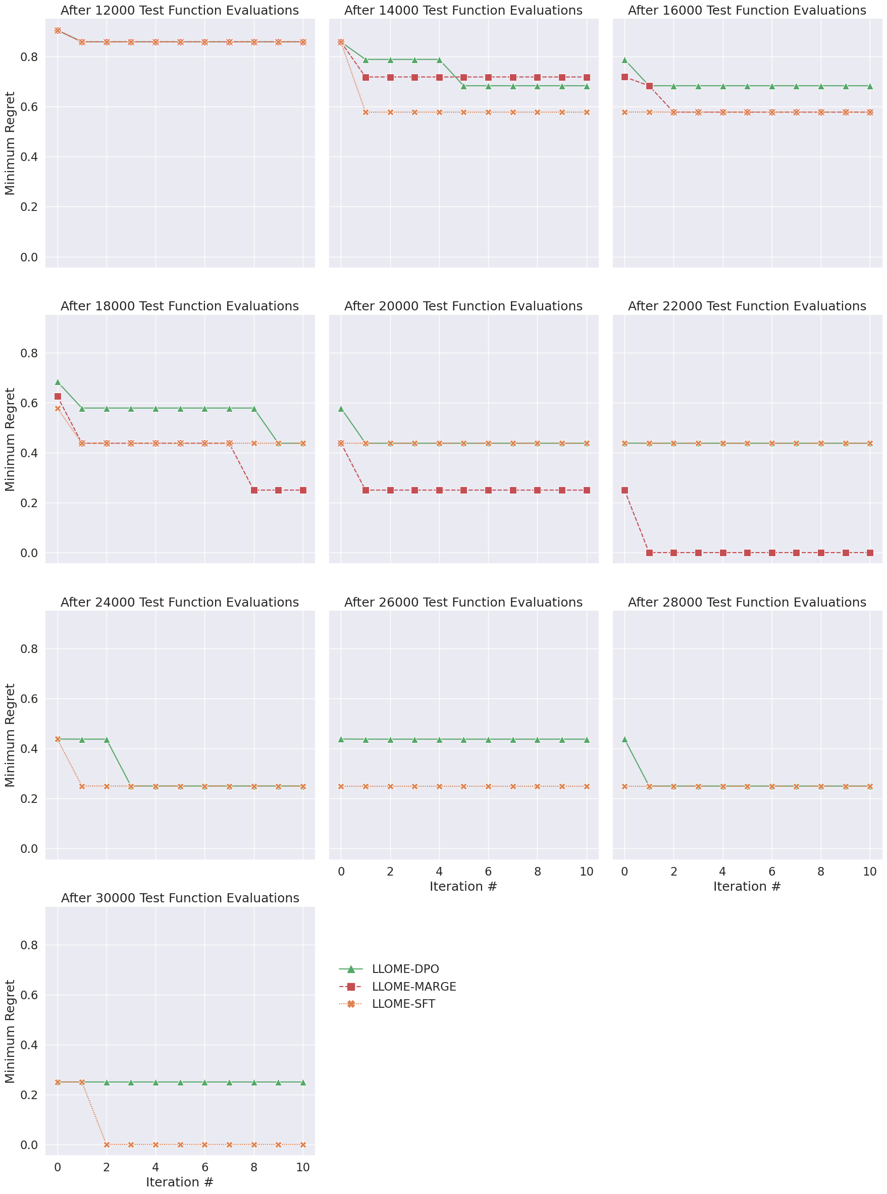
Figure 13: Minimum regret of sequences generated during the LLM inner loop, at each iteration of the iterative refinement process. The titles reflect the number of oracle labels that each LLM has been trained on. These plots account for all generations sampled from the LLM inner loop, and not just the samples selected via likelihood selection, as in Alg. 3.

References

- AhmadiTeshnizi et al. [2024] Ali AhmadiTeshnizi, Wenzhi Gao, and Madeleine Udell. Optimus: Scalable optimization modeling with (mi) lp solvers and large language models. arXiv preprint arXiv:2402.10172, 2024.
- Ahmed & Choudhury [2024] Tasnim Ahmed and Salimur Choudhury. Lm4opt: Unveiling the potential of large language models in formulating mathematical optimization problems, 2024. URL https://arxiv.org/abs/2403.01342.
- Amin & Neumann [2021] Saadullah Amin and Guenter Neumann. T2NER: Transformers based transfer learning framework for named entity recognition. In Dimitra Gkatzia and Djamé Seddah (eds.), Proceedings of the 16th Conference of the European Chapter of the Association for Computational Linguistics: System Demonstrations, pp. 212–220, Online, April 2021. Association for Computational Linguistics. doi: 10.18653/v1/2021.eacl-demos.25. URL https://aclanthology.org/2021.eacl-demos.25.
- Angermueller et al. [2020] Christof Angermueller, David Belanger, Andreea Gane, Zelda Mariet, David Dohan, Kevin Murphy, Lucy Colwell, and D Sculley. Population-based black-box optimization for biological sequence design. In International conference on machine learning, pp. 324–334. PMLR, 2020.
- Arkhipov et al. [2019] Mikhail Arkhipov, Maria Trofimova, Yuri Kuratov, and Alexey Sorokin. Tuning multilingual transformers for language-specific named entity recognition. In Tomaž Erjavec, Michał Marcińczuk, Preslav Nakov, Jakub Piskorski, Lidia Pivovarova, Jan Šnajder, Josef Steinberger, and Roman Yangarber (eds.), Proceedings of the 7th Workshop on Balto-Slavic Natural Language Processing, pp. 89–93, Florence, Italy, August 2019. Association for Computational Linguistics. doi: 10.18653/v1/W19-3712. URL https://aclanthology.org/W19-3712.
- Arnold [1998] Frances H Arnold. Design by directed evolution. Accounts of chemical research, 31(3):125–131, 1998.
- Back [1996] Thomas Back. Evolutionary algorithms in theory and practice: evolution strategies, evolutionary programming, genetic algorithms. Oxford university press, 1996.
- Barlow et al. [2018] Kyle A Barlow, Shane O Conchuir, Samuel Thompson, Pooja Suresh, James E Lucas, Markus Heinonen, and Tanja Kortemme. Flex ddg: Rosetta ensemble-based estimation of changes in protein–protein binding affinity upon mutation. The Journal of Physical Chemistry B, 122(21):5389–5399, 2018.
- Biderman et al. [2023] Stella Biderman, Hailey Schoelkopf, Quentin Gregory Anthony, Herbie Bradley, Kyle O’Brien, Eric Hallahan, Mohammad Aflah Khan, Shivanshu Purohit, USVSN Sai Prashanth, Edward Raff, et al. Pythia: A suite for analyzing large language models across training and scaling. In International Conference on Machine Learning, pp. 2397–2430. PMLR, 2023.
- Bommasani et al. [2021] Rishi Bommasani, Drew A. Hudson, Ehsan Adeli, Russ Altman, Simran Arora, Sydney von Arx, Michael S. Bernstein, Jeannette Bohg, Antoine Bosselut, Emma Brunskill, Erik Brynjolfsson, S. Buch, Dallas Card, Rodrigo Castellon, Niladri S. Chatterji, Annie S. Chen, Kathleen A. Creel, Jared Davis, Dora Demszky, Chris Donahue, Moussa Doumbouya, Esin Durmus, Stefano Ermon, John Etchemendy, Kawin Ethayarajh, Li Fei-Fei, Chelsea Finn, Trevor Gale, Lauren E. Gillespie, Karan Goel, Noah D. Goodman, Shelby Grossman, Neel Guha, Tatsunori Hashimoto, Peter Henderson, John Hewitt, Daniel E. Ho, Jenny Hong, Kyle Hsu, Jing Huang, Thomas F. Icard, Saahil Jain, Dan Jurafsky, Pratyusha Kalluri, Siddharth Karamcheti, Geoff Keeling, Fereshte Khani, O. Khattab, Pang Wei Koh, Mark S. Krass, Ranjay Krishna, Rohith Kuditipudi, Ananya Kumar, Faisal Ladhak, Mina Lee, Tony Lee, Jure Leskovec, Isabelle Levent, Xiang Lisa Li, Xuechen Li, Tengyu Ma, Ali Malik, Christopher D. Manning, Suvir P. Mirchandani, Eric Mitchell, Zanele Munyikwa, Suraj Nair, Avanika Narayan, Deepak Narayanan, Benjamin Newman, Allen Nie, Juan Carlos Niebles, Hamed Nilforoshan, J. F. Nyarko, Giray Ogut, Laurel Orr, Isabel Papadimitriou, Joon Sung Park, Chris Piech, Eva Portelance, Christopher Potts, Aditi Raghunathan, Robert Reich, Hongyu Ren, Frieda Rong, Yusuf H. Roohani, Camilo Ruiz, Jack Ryan, Christopher R’e, Dorsa Sadigh, Shiori Sagawa, Keshav Santhanam, Andy Shih, Krishna Parasuram Srinivasan, Alex Tamkin, Rohan Taori, Armin W. Thomas, Florian Tramèr, Rose E. Wang, William Wang, Bohan Wu, Jiajun Wu, Yuhuai Wu, Sang Michael Xie, Michihiro Yasunaga, Jiaxuan You, Matei A. Zaharia, Michael Zhang, Tianyi Zhang, Xikun Zhang, Yuhui Zhang, Lucia Zheng, Kaitlyn Zhou, and Percy Liang. On the opportunities and risks of foundation models. ArXiv, 2021. URL https://crfm.stanford.edu/assets/report.pdf.
- Brown et al. [2020] Tom Brown, Benjamin Mann, Nick Ryder, Melanie Subbiah, Jared D Kaplan, Prafulla Dhariwal, Arvind Neelakantan, Pranav Shyam, Girish Sastry, Amanda Askell, Sandhini Agarwal, Ariel Herbert-Voss, Gretchen Krueger, Tom Henighan, Rewon Child, Aditya Ramesh, Daniel Ziegler, Jeffrey Wu, Clemens Winter, Chris Hesse, Mark Chen, Eric Sigler, Mateusz Litwin, Scott Gray, Benjamin Chess, Jack Clark, Christopher Berner, Sam McCandlish, Alec Radford, Ilya Sutskever, and Dario Amodei. Language models are few-shot learners. In H. Larochelle, M. Ranzato, R. Hadsell, M.F. Balcan, and H. Lin (eds.), Advances in Neural Information Processing Systems, volume 33, pp. 1877–1901. Curran Associates, Inc., 2020. URL https://proceedings.neurips.cc/paper_files/paper/2020/file/1457c0d6bfcb4967418bfb8ac142f64a-Paper.pdf.
- Carlsson et al. [2022] Fredrik Carlsson, Joey Öhman, Fangyu Liu, Severine Verlinden, Joakim Nivre, and Magnus Sahlgren. Fine-grained controllable text generation using non-residual prompting. In Smaranda Muresan, Preslav Nakov, and Aline Villavicencio (eds.), Proceedings of the 60th Annual Meeting of the Association for Computational Linguistics (Volume 1: Long Papers), pp. 6837–6857, Dublin, Ireland, May 2022. Association for Computational Linguistics. doi: 10.18653/v1/2022.acl-long.471. URL https://aclanthology.org/2022.acl-long.471.
- Casper et al. [2023] Stephen Casper, Xander Davies, Claudia Shi, Thomas Krendl Gilbert, Jérémy Scheurer, Javier Rando, Rachel Freedman, Tomasz Korbak, David Lindner, Pedro Freire, Tony Wang, Samuel Marks, Charbel-Raphaël Segerie, Micah Carroll, Andi Peng, Phillip Christoffersen, Mehul Damani, Stewart Slocum, Usman Anwar, Anand Siththaranjan, Max Nadeau, Eric J. Michaud, Jacob Pfau, Dmitrii Krasheninnikov, Xin Chen, Lauro Langosco, Peter Hase, Erdem Bıyık, Anca Dragan, David Krueger, Dorsa Sadigh, and Dylan Hadfield-Menell. Open problems and fundamental limitations of reinforcement learning from human feedback, 2023. URL https://arxiv.org/abs/2307.15217.
- Chan et al. [2021] Alvin Chan, Ali Madani, Ben Krause, and Nikhil Naik. Deep extrapolation for attribute-enhanced generation. In M. Ranzato, A. Beygelzimer, Y. Dauphin, P.S. Liang, and J. Wortman Vaughan (eds.), Advances in Neural Information Processing Systems, volume 34, pp. 14084–14096. Curran Associates, Inc., 2021. URL https://proceedings.neurips.cc/paper_files/paper/2021/file/75da5036f659fe64b53f3d9b39412967-Paper.pdf.
- Chen et al. [2024a] Angelica Chen, David M. Dohan, and David R. So. Evoprompting: language models for code-level neural architecture search. In Proceedings of the 37th International Conference on Neural Information Processing Systems, NIPS ’23, Red Hook, NY, USA, 2024a. Curran Associates Inc.
- Chen et al. [2024b] Angelica Chen, Sadhika Malladi, Lily H. Zhang, Xinyi Chen, Qiuyi Zhang, Rajesh Ranganath, and Kyunghyun Cho. Preference learning algorithms do not learn preference rankings. arXiv preprint arXiv:2405.19534, 2024b. URL https://arxiv.org/abs/2405.19534.
- Chen et al. [2021] Mark Chen, Jerry Tworek, Heewoo Jun, Qiming Yuan, Henrique Ponde De Oliveira Pinto, Jared Kaplan, Harri Edwards, Yuri Burda, Nicholas Joseph, Greg Brockman, et al. Evaluating large language models trained on code. arXiv preprint arXiv:2107.03374, 2021.
- Chen et al. [2022a] Xiaoxue Chen, Tianyu Liu, Hao Zhao, Guyue Zhou, and Ya-Qin Zhang. Cerberus transformer: Joint semantic, affordance and attribute parsing. In Proceedings of the IEEE/CVF Conference on Computer Vision and Pattern Recognition, pp. 19649–19658, 2022a.
- Chen et al. [2024c] Yihan Chen, Benfeng Xu, Quan Wang, Yi Liu, and Zhendong Mao. Benchmarking large language models on controllable generation under diversified instructions. Proceedings of the AAAI Conference on Artificial Intelligence, 38(16):17808–17816, Mar. 2024c. doi: 10.1609/aaai.v38i16.29734. URL https://ojs.aaai.org/index.php/AAAI/article/view/29734.
- Chen et al. [2022b] Yutian Chen, Xingyou Song, Chansoo Lee, Zi Wang, Richard Zhang, David Dohan, Kazuya Kawakami, Greg Kochanski, Arnaud Doucet, Marc' Aurelio Ranzato, Sagi Perel, and Nando de Freitas. Towards learning universal hyperparameter optimizers with transformers. In S. Koyejo, S. Mohamed, A. Agarwal, D. Belgrave, K. Cho, and A. Oh (eds.), Advances in Neural Information Processing Systems, volume 35, pp. 32053–32068. Curran Associates, Inc., 2022b. URL https://proceedings.neurips.cc/paper_files/paper/2022/file/cf6501108fced72ee5c47e2151c4e153-Paper-Conference.pdf.
- Cieplinski et al. [2023] Tobiasz Cieplinski, Tomasz Danel, Sabina Podlewska, and Stanisław Jastrzebski. Generative models should at least be able to design molecules that dock well: A new benchmark. Journal of Chemical Information and Modeling, 63(11):3238–3247, 2023.
- Dathathri et al. [2020] Sumanth Dathathri, Andrea Madotto, Janice Lan, Jane Hung, Eric Frank, Piero Molino, Jason Yosinski, and Rosanne Liu. Plug and play language models: A simple approach to controlled text generation. In International Conference on Learning Representations, 2020. URL https://openreview.net/forum?id=H1edEyBKDS.
- Dekoninck et al. [2024] Jasper Dekoninck, Marc Fischer, Luca Beurer-Kellner, and Martin Vechev. Controlled text generation via language model arithmetic. In The Twelfth International Conference on Learning Representations, 2024. URL https://openreview.net/forum?id=SLw9fp4yI6.
- Deng & Raffel [2023] Haikang Deng and Colin Raffel. Reward-augmented decoding: Efficient controlled text generation with a unidirectional reward model. In Houda Bouamor, Juan Pino, and Kalika Bali (eds.), Proceedings of the 2023 Conference on Empirical Methods in Natural Language Processing, pp. 11781–11791, Singapore, December 2023. Association for Computational Linguistics. doi: 10.18653/v1/2023.emnlp-main.721. URL https://aclanthology.org/2023.emnlp-main.721.
- Doan [2022] Xuan-Dung Doan. Vtcc-nlp at nl4opt competition subtask 1: An ensemble pre-trained language models for named entity recognition, 2022. URL https://arxiv.org/abs/2212.07219.
- Dong et al. [2023] Hanze Dong, Wei Xiong, Deepanshu Goyal, Yihan Zhang, Winnie Chow, Rui Pan, Shizhe Diao, Jipeng Zhang, KaShun SHUM, and Tong Zhang. RAFT: Reward ranked finetuning for generative foundation model alignment. Transactions on Machine Learning Research, 2023. ISSN 2835-8856. URL https://openreview.net/forum?id=m7p5O7zblY.
- Drozdov et al. [2023] Andrew Drozdov, Nathanael Schärli, Ekin Akyürek, Nathan Scales, Xinying Song, Xinyun Chen, Olivier Bousquet, and Denny Zhou. Compositional semantic parsing with large language models. In The Eleventh International Conference on Learning Representations, 2023. URL https://openreview.net/forum?id=gJW8hSGBys8.
- Du et al. [2023] Li Du, Lucas Torroba Hennigen, Tiago Pimentel, Clara Meister, Jason Eisner, and Ryan Cotterell. A measure-theoretic characterization of tight language models. In Anna Rogers, Jordan Boyd-Graber, and Naoaki Okazaki (eds.), Proceedings of the 61st Annual Meeting of the Association for Computational Linguistics (Volume 1: Long Papers), pp. 9744–9770, Toronto, Canada, July 2023. Association for Computational Linguistics. doi: 10.18653/v1/2023.acl-long.543. URL https://aclanthology.org/2023.acl-long.543.
- Feng et al. [2024] Duanyu Feng, Bowen Qin, Chen Huang, Zheng Zhang, and Wenqiang Lei. Towards analyzing and understanding the limitations of dpo: A theoretical perspective, 2024. URL https://arxiv.org/abs/2404.04626.
- Gao et al. [2022] Luyu Gao, Aman Madaan, Shuyan Zhou, Uri Alon, Pengfei Liu, Yiming Yang, Jamie Callan, and Graham Neubig. Pal: Program-aided language models. arXiv preprint arXiv:2211.10435, 2022.
- Garbacea & Mei [2022] Cristina Garbacea and Qiaozhu Mei. Why is constrained neural language generation particularly challenging?, 2022.
- Gruver et al. [2024] Nate Gruver, Samuel Stanton, Nathan Frey, Tim GJ Rudner, Isidro Hotzel, Julien Lafrance-Vanasse, Arvind Rajpal, Kyunghyun Cho, and Andrew G Wilson. Protein design with guided discrete diffusion. Advances in neural information processing systems, 36, 2024.
- Guo et al. [2024a] Pei-Fu Guo, Ying-Hsuan Chen, Yun-Da Tsai, and Shou-De Lin. Towards optimizing with large language models. In Fourth Workshop on Knowledge-infused Learning, 2024a. URL https://openreview.net/forum?id=vIU8LUckb4.
- Guo et al. [2024b] Qingyan Guo, Rui Wang, Junliang Guo, Bei Li, Kaitao Song, Xu Tan, Guoqing Liu, Jiang Bian, and Yujiu Yang. Connecting large language models with evolutionary algorithms yields powerful prompt optimizers. In The Twelfth International Conference on Learning Representations, 2024b. URL https://openreview.net/forum?id=ZG3RaNIsO8.
- Guo et al. [2024c] Zixian Guo, Ming Liu, Zhilong Ji, Jinfeng Bai, Yiwen Guo, and Wangmeng Zuo. Two optimizers are better than one: Llm catalyst empowers gradient-based optimization for prompt tuning, 2024c. URL https://arxiv.org/abs/2405.19732.
- Gupta et al. [2018] Sonal Gupta, Rushin Shah, Mrinal Mohit, Anuj Kumar, and Mike Lewis. Semantic parsing for task oriented dialog using hierarchical representations. arXiv preprint arXiv:1810.07942, 2018.
- He et al. [2022] JiangLong He, Mamatha N, Shiv Vignesh, Deepak Kumar, and Akshay Uppal. Linear programming word problems formulation using ensemblecrf ner labeler and t5 text generator with data augmentations, 2022. URL https://arxiv.org/abs/2212.14657.
- He-Yueya et al. [2023] Joy He-Yueya, Gabriel Poesia, Rose E Wang, and Noah D Goodman. Solving math word problems by combining language models with symbolic solvers. arXiv preprint arXiv:2304.09102, 2023.
- Hu et al. [2024] Xiangkun Hu, Tong He, and David Wipf. New desiderata for direct preference optimization. In ICML 2024 Workshop on Models of Human Feedback for AI Alignment, 2024. URL https://openreview.net/forum?id=Fgf0iAOb22.
- Hummer et al. [2023] Alissa M Hummer, Constantin Schneider, Lewis Chinery, and Charlotte M Deane. Investigating the volume and diversity of data needed for generalizable antibody-antigen g prediction. bioRxiv, pp. 2023–05, 2023.
- Jang [2022] Sanghwan Jang. Tag embedding and well-defined intermediate representation improve auto-formulation of problem description. arXiv preprint arXiv:2212.03575, 2022.
- Kellogg et al. [2011] Elizabeth H Kellogg, Andrew Leaver-Fay, and David Baker. Role of conformational sampling in computing mutation-induced changes in protein structure and stability. Proteins: Structure, Function, and Bioinformatics, 79(3):830–838, 2011.
- Keskar et al. [2019] Nitish Shirish Keskar, Bryan McCann, Lav Varshney, Caiming Xiong, and Richard Socher. CTRL - A Conditional Transformer Language Model for Controllable Generation. arXiv preprint arXiv:1909.05858, 2019.
- Khattab et al. [2024] Omar Khattab, Arnav Singhvi, Paridhi Maheshwari, Zhiyuan Zhang, Keshav Santhanam, Sri Vardhamanan A, Saiful Haq, Ashutosh Sharma, Thomas T. Joshi, Hanna Moazam, Heather Miller, Matei Zaharia, and Christopher Potts. DSPy: Compiling declarative language model calls into state-of-the-art pipelines. In The Twelfth International Conference on Learning Representations, 2024. URL https://openreview.net/forum?id=sY5N0zY5Od.
- Kirk et al. [2024] Robert Kirk, Ishita Mediratta, Christoforos Nalmpantis, Jelena Luketina, Eric Hambro, Edward Grefenstette, and Roberta Raileanu. Understanding the effects of RLHF on LLM generalisation and diversity. In The Twelfth International Conference on Learning Representations, 2024. URL https://openreview.net/forum?id=PXD3FAVHJT.
- Korbak et al. [2022a] Tomasz Korbak, Hady Elsahar, Germán Kruszewski, and Marc Dymetman. On reward maximization and distribution matching for fine-tuning language models, 2022a. URL https://openreview.net/forum?id=8f95ajHrIFc.
- Korbak et al. [2022b] Tomasz Korbak, Ethan Perez, and Christopher L Buckley. Rl with kl penalties is better viewed as bayesian inference, 2022b. URL https://arxiv.org/abs/2205.11275.
- Lange et al. [2024] Robert Lange, Yingtao Tian, and Yujin Tang. Large language models as evolution strategies. In Proceedings of the Genetic and Evolutionary Computation Conference Companion, GECCO ’24 Companion, pp. 579–582, New York, NY, USA, 2024. Association for Computing Machinery. ISBN 9798400704956. doi: 10.1145/3638530.3654238. URL https://doi.org/10.1145/3638530.3654238.
- Lehman et al. [2023] Joel Lehman, Jonathan Gordon, Shawn Jain, Kamal Ndousse, Cathy Yeh, and Kenneth O Stanley. Evolution through large models. In Handbook of Evolutionary Machine Learning, pp. 331–366. Springer, 2023.
- Li et al. [2024] Haolong Li, Yu Ma, Yinqi Zhang, Chen Ye, and Jie Chen. Exploring mathematical extrapolation of large language models with synthetic data. In Lun-Wei Ku, Andre Martins, and Vivek Srikumar (eds.), Findings of the Association for Computational Linguistics ACL 2024, pp. 936–946, Bangkok, Thailand and virtual meeting, August 2024. Association for Computational Linguistics. doi: 10.18653/v1/2024.findings-acl.55. URL https://aclanthology.org/2024.findings-acl.55.
- Liu et al. [2021] Alisa Liu, Maarten Sap, Ximing Lu, Swabha Swayamdipta, Chandra Bhagavatula, Noah A. Smith, and Yejin Choi. DExperts: Decoding-time controlled text generation with experts and anti-experts. In Chengqing Zong, Fei Xia, Wenjie Li, and Roberto Navigli (eds.), Proceedings of the 59th Annual Meeting of the Association for Computational Linguistics and the 11th International Joint Conference on Natural Language Processing (Volume 1: Long Papers), pp. 6691–6706, Online, August 2021. Association for Computational Linguistics. doi: 10.18653/v1/2021.acl-long.522. URL https://aclanthology.org/2021.acl-long.522.
- Liu et al. [2024a] Shengcai Liu, Caishun Chen, Xinghua Qu, Ke Tang, and Yew-Soon Ong. Large language models as evolutionary optimizers. In 2024 IEEE Congress on Evolutionary Computation (CEC), pp. 1–8, 2024a. doi: 10.1109/CEC60901.2024.10611913.
- Liu et al. [2024b] Tennison Liu, Nicolás Astorga, Nabeel Seedat, and Mihaela van der Schaar. Large language models to enhance bayesian optimization. arXiv preprint arXiv:2402.03921, 2024b.
- Ma et al. [2024] Pingchuan Ma, Tsun-Hsuan Wang, Minghao Guo, Zhiqing Sun, Joshua B. Tenenbaum, Daniela Rus, Chuang Gan, and Wojciech Matusik. LLM and simulation as bilevel optimizers: A new paradigm to advance physical scientific discovery. In Ruslan Salakhutdinov, Zico Kolter, Katherine Heller, Adrian Weller, Nuria Oliver, Jonathan Scarlett, and Felix Berkenkamp (eds.), Proceedings of the 41st International Conference on Machine Learning, volume 235 of Proceedings of Machine Learning Research, pp. 33940–33962. PMLR, 21–27 Jul 2024. URL https://proceedings.mlr.press/v235/ma24m.html.
- Madaan et al. [2024] Aman Madaan, Niket Tandon, Prakhar Gupta, Skyler Hallinan, Luyu Gao, Sarah Wiegreffe, Uri Alon, Nouha Dziri, Shrimai Prabhumoye, Yiming Yang, et al. Self-refine: Iterative refinement with self-feedback. Advances in Neural Information Processing Systems, 36, 2024.
- Madani et al. [2023] Ali Madani, Ben Krause, Eric R. Greene, Subu Subramanian, Benjamin P. Mohr, James M. Holton, Jose Luis Olmos, Caiming Xiong, Zachary Z. Sun, Richard Socher, James S. Fraser, and Nikhil Naik. Large language models generate functional protein sequences across diverse families. Nature Biotechnology, 41(8):1099–1106, January 2023. ISSN 1546-1696. doi: 10.1038/s41587-022-01618-2. URL http://dx.doi.org/10.1038/s41587-022-01618-2.
- Malladi [2024] Sadhika Malladi. The hidden infinity in preference learning, July 2024. URL https://www.cs.princeton.edu/~smalladi/blog/2024/06/27/dpo-infinity/.
- Maus et al. [2022] Natalie Maus, Haydn Jones, Juston Moore, Matt J Kusner, John Bradshaw, and Jacob Gardner. Local latent space bayesian optimization over structured inputs. Advances in neural information processing systems, 35:34505–34518, 2022.
- Meng et al. [2024] Yu Meng, Mengzhou Xia, and Danqi Chen. SimPO: Simple preference optimization with a reference-free reward. arXiv preprint arXiv:2405.14734, 2024.
- Meyerson et al. [2024] Elliot Meyerson, Mark J. Nelson, Herbie Bradley, Adam Gaier, Arash Moradi, Amy K. Hoover, and Joel Lehman. Language model crossover: Variation through few-shot prompting. ACM Trans. Evol. Learn. Optim., September 2024. doi: 10.1145/3694791. URL https://doi.org/10.1145/3694791. Just Accepted.
- Mittal et al. [2024] Chinmay Mittal, Krishna Kartik, Mausam, and Parag Singla. Puzzlebench: Can llms solve challenging first-order combinatorial reasoning problems?, 2024. URL https://arxiv.org/abs/2402.02611.
- Molga & Smutnicki [2005] Marcin Molga and Czesław Smutnicki. Test functions for optimization needs. Test functions for optimization needs, 101:48, 2005.
- Nasir et al. [2024] Muhammad Umair Nasir, Sam Earle, Julian Togelius, Steven James, and Christopher Cleghorn. Llmatic: neural architecture search via large language models and quality diversity optimization. In Proceedings of the Genetic and Evolutionary Computation Conference, pp. 1110–1118, 2024.
- Nie et al. [2023] Allen Nie, Ching-An Cheng, Andrey Kolobov, and Adith Swaminathan. Importance of directional feedback for LLM-based optimizers. In NeurIPS 2023 Foundation Models for Decision Making Workshop, 2023. URL https://openreview.net/forum?id=QW4eGh5GT3.
- Nijkamp et al. [2023a] Erik Nijkamp, Hiroaki Hayashi, Caiming Xiong, Silvio Savarese, and Yingbo Zhou. Codegen2: Lessons for training llms on programming and natural languages. ICLR, 2023a.
- Nijkamp et al. [2023b] Erik Nijkamp, Bo Pang, Hiroaki Hayashi, Lifu Tu, Huan Wang, Yingbo Zhou, Silvio Savarese, and Caiming Xiong. Codegen: An open large language model for code with multi-turn program synthesis. ICLR, 2023b.
- Ning et al. [2023] Yuting Ning, Jiayu Liu, Longhu Qin, Tong Xiao, Shangzi Xue, Zhenya Huang, Qi Liu, Enhong Chen, and Jinze Wu. A novel approach for auto-formulation of optimization problems. arXiv preprint arXiv:2302.04643, 2023.
- Owen [2013] Art B. Owen. Monte Carlo theory, methods and examples. https://artowen.su.domains/mc/, 2013.
- Padmakumar & He [2024] Vishakh Padmakumar and He He. Does writing with language models reduce content diversity?, 2024. URL https://arxiv.org/abs/2309.05196.
- Padmakumar et al. [2023] Vishakh Padmakumar, Richard Yuanzhe Pang, He He, and Ankur P Parikh. Extrapolative controlled sequence generation via iterative refinement. In International Conference on Machine Learning, pp. 26792–26808. PMLR, 2023.
- Pal et al. [2024] Arka Pal, Deep Karkhanis, Samuel Dooley, Manley Roberts, Siddartha Naidu, and Colin White. Smaug: Fixing failure modes of preference optimisation with dpo-positive, 2024. URL https://arxiv.org/abs/2402.13228.
- Pang et al. [2024] Richard Yuanzhe Pang, Weizhe Yuan, Kyunghyun Cho, He He, Sainbayar Sukhbaatar, and Jason Weston. Iterative reasoning preference optimization, 2024. URL https://arxiv.org/abs/2404.19733.
- Pascual et al. [2021] Damian Pascual, Beni Egressy, Clara Meister, Ryan Cotterell, and Roger Wattenhofer. A plug-and-play method for controlled text generation. In Marie-Francine Moens, Xuanjing Huang, Lucia Specia, and Scott Wen-tau Yih (eds.), Findings of the Association for Computational Linguistics: EMNLP 2021, pp. 3973–3997, Punta Cana, Dominican Republic, November 2021. Association for Computational Linguistics. doi: 10.18653/v1/2021.findings-emnlp.334. URL https://aclanthology.org/2021.findings-emnlp.334.
- Paszke et al. [2019] Adam Paszke, Sam Gross, Francisco Massa, Adam Lerer, James Bradbury, Gregory Chanan, Trevor Killeen, Zeming Lin, Natalia Gimelshein, Luca Antiga, et al. Pytorch: An imperative style, high-performance deep learning library. Advances in neural information processing systems, 32, 2019.
- Poesia et al. [2022] Gabriel Poesia, Alex Polozov, Vu Le, Ashish Tiwari, Gustavo Soares, Christopher Meek, and Sumit Gulwani. Synchromesh: Reliable code generation from pre-trained language models. In International Conference on Learning Representations, 2022. URL https://openreview.net/forum?id=KmtVD97J43e.
- Press et al. [2022] Ofir Press, Noah Smith, and Mike Lewis. Train short, test long: Attention with linear biases enables input length extrapolation. In International Conference on Learning Representations, 2022. URL https://openreview.net/forum?id=R8sQPpGCv0.
- Pryzant et al. [2023] Reid Pryzant, Dan Iter, Jerry Li, Yin Lee, Chenguang Zhu, and Michael Zeng. Automatic prompt optimization with “gradient descent” and beam search. In Houda Bouamor, Juan Pino, and Kalika Bali (eds.), Proceedings of the 2023 Conference on Empirical Methods in Natural Language Processing, pp. 7957–7968, Singapore, December 2023. Association for Computational Linguistics. doi: 10.18653/v1/2023.emnlp-main.494. URL https://aclanthology.org/2023.emnlp-main.494.
- Radford et al. [2019] Alec Radford, Jeff Wu, Rewon Child, David Luan, Dario Amodei, and Ilya Sutskever. Language models are unsupervised multitask learners. 2019.
- Rafailov et al. [2023] Rafael Rafailov, Archit Sharma, Eric Mitchell, Christopher D Manning, Stefano Ermon, and Chelsea Finn. Direct preference optimization: Your language model is secretly a reward model. In Thirty-seventh Conference on Neural Information Processing Systems, 2023. URL https://openreview.net/forum?id=HPuSIXJaa9.
- Rafailov et al. [2024a] Rafael Rafailov, Yaswanth Chittepu, Ryan Park, Harshit Sikchi, Joey Hejna, Bradley Knox, Chelsea Finn, and Scott Niekum. Scaling laws for reward model overoptimization in direct alignment algorithms, 2024a. URL https://arxiv.org/abs/2406.02900.
- Rafailov et al. [2024b] Rafael Rafailov, Joey Hejna, Ryan Park, and Chelsea Finn. From $r$ to $q^*$: Your language model is secretly a q-function. In First Conference on Language Modeling, 2024b. URL https://openreview.net/forum?id=kEVcNxtqXk.
- Raffel et al. [2020] Colin Raffel, Noam Shazeer, Adam Roberts, Katherine Lee, Sharan Narang, Michael Matena, Yanqi Zhou, Wei Li, and Peter J. Liu. Exploring the limits of transfer learning with a unified text-to-text transformer. J. Mach. Learn. Res., 21(1), January 2020. ISSN 1532-4435.
- Ramamonjison et al. [2022] Rindranirina Ramamonjison, Timothy Yu, Raymond Li, Haley Li, Giuseppe Carenini, Bissan Ghaddar, Shiqi He, Mahdi Mostajabdaveh, Amin Banitalebi-Dehkordi, Zirui Zhou, and Yong Zhang. Nl4opt competition: Formulating optimization problems based on their natural language descriptions. In Marco Ciccone, Gustavo Stolovitzky, and Jacob Albrecht (eds.), Proceedings of the NeurIPS 2022 Competitions Track, volume 220 of Proceedings of Machine Learning Research, pp. 189–203. PMLR, 28 Nov–09 Dec 2022. URL https://proceedings.mlr.press/v220/ramamonjison23a.html.
- Romera-Paredes et al. [2023] Bernardino Romera-Paredes, Mohammadamin Barekatain, Alexander Novikov, Matej Balog, M. Pawan Kumar, Emilien Dupont, Francisco J. R. Ruiz, Jordan S. Ellenberg, Pengming Wang, Omar Fawzi, Pushmeet Kohli, and Alhussein Fawzi. Mathematical discoveries from program search with large language models. Nature, 625(7995):468–475, December 2023. ISSN 1476-4687. doi: 10.1038/s41586-023-06924-6. URL http://dx.doi.org/10.1038/s41586-023-06924-6.
- Rongali et al. [2020] Subendhu Rongali, Luca Soldaini, Emilio Monti, and Wael Hamza. Don’t parse, generate! a sequence to sequence architecture for task-oriented semantic parsing. In Proceedings of the web conference 2020, pp. 2962–2968, 2020.
- Shao et al. [2020] Bo Shao, Yeyun Gong, Weizhen Qi, Guihong Cao, Jianshu Ji, and Xiaola Lin. Graph-based transformer with cross-candidate verification for semantic parsing. In Proceedings of the AAAI Conference on Artificial Intelligence, volume 34, pp. 8807–8814, 2020.
- Shaw et al. [2019] Peter Shaw, Philip Massey, Angelica Chen, Francesco Piccinno, and Yasemin Altun. Generating logical forms from graph representations of text and entities. In Anna Korhonen, David Traum, and Lluís Màrquez (eds.), Proceedings of the 57th Annual Meeting of the Association for Computational Linguistics, pp. 95–106, Florence, Italy, July 2019. Association for Computational Linguistics. doi: 10.18653/v1/P19-1010. URL https://aclanthology.org/P19-1010.
- Shi et al. [2021] Peng Shi, Patrick Ng, Zhiguo Wang, Henghui Zhu, Alexander Hanbo Li, Jun Wang, Cicero Nogueira dos Santos, and Bing Xiang. Learning contextual representations for semantic parsing with generation-augmented pre-training. In Proceedings of the AAAI Conference on Artificial Intelligence, volume 35, pp. 13806–13814, 2021.
- Sinai et al. [2020] Sam Sinai, Richard Wang, Alexander Whatley, Stewart Slocum, Elina Locane, and Eric D Kelsic. Adalead: A simple and robust adaptive greedy search algorithm for sequence design. arXiv preprint arXiv:2010.02141, 2020.
- Singhal et al. [2024] Prasann Singhal, Tanya Goyal, Jiacheng Xu, and Greg Durrett. A long way to go: Investigating length correlations in RLHF, 2024. URL https://openreview.net/forum?id=sNtDKdcI1f.
- Song et al. [2024] Xingyou Song, Yingtao Tian, Robert Tjarko Lange, Chansoo Lee, Yujin Tang, and Yutian Chen. Position: Leverage foundational models for black-box optimization. In Forty-first International Conference on Machine Learning, 2024. URL https://openreview.net/forum?id=ea2MgKn3sV.
- Stanton et al. [2022] Samuel Stanton, Wesley Maddox, Nate Gruver, Phillip Maffettone, Emily Delaney, Peyton Greenside, and Andrew Gordon Wilson. Accelerating bayesian optimization for biological sequence design with denoising autoencoders. In International Conference on Machine Learning, pp. 20459–20478. PMLR, 2022.
- Stengel-Eskin et al. [2021] Elias Stengel-Eskin, Kenton Murray, Sheng Zhang, Aaron Steven White, and Benjamin Van Durme. Joint universal syntactic and semantic parsing. Transactions of the Association for Computational Linguistics, 9:756–773, 2021.
- Stiennon et al. [2020] Nisan Stiennon, Long Ouyang, Jeffrey Wu, Daniel Ziegler, Ryan Lowe, Chelsea Voss, Alec Radford, Dario Amodei, and Paul F Christiano. Learning to summarize with human feedback. In H. Larochelle, M. Ranzato, R. Hadsell, M.F. Balcan, and H. Lin (eds.), Advances in Neural Information Processing Systems, volume 33, pp. 3008–3021. Curran Associates, Inc., 2020. URL https://proceedings.neurips.cc/paper_files/paper/2020/file/1f89885d556929e98d3ef9b86448f951-Paper.pdf.
- Sun et al. [2023] Jiao Sun, Yufei Tian, Wangchunshu Zhou, Nan Xu, Qian Hu, Rahul Gupta, John Wieting, Nanyun Peng, and Xuezhe Ma. Evaluating large language models on controlled generation tasks. In Houda Bouamor, Juan Pino, and Kalika Bali (eds.), Proceedings of the 2023 Conference on Empirical Methods in Natural Language Processing, pp. 3155–3168, Singapore, December 2023. Association for Computational Linguistics. doi: 10.18653/v1/2023.emnlp-main.190. URL https://aclanthology.org/2023.emnlp-main.190.
- Tagasovska et al. [2024] Nataša Tagasovska, Vladimir Gligorijević, Kyunghyun Cho, and Andreas Loukas. Implicitly guided design with propen: Match your data to follow the gradient, 2024. URL https://arxiv.org/abs/2405.18075.
- Tang et al. [2024] Yunhao Tang, Daniel Zhaohan Guo, Zeyu Zheng, Daniele Calandriello, Yuan Cao, Eugene Tarassov, Rémi Munos, Bernardo Ávila Pires, Michal Valko, Yong Cheng, and Will Dabney. Understanding the performance gap between online and offline alignment algorithms, 2024. URL https://arxiv.org/abs/2405.08448.
- Tripp et al. [2021] Austin Tripp, Gregor N. C. Simm, and José Miguel Hernández-Lobato. A fresh look at de novo molecular design benchmarks. In NeurIPS 2021 AI for Science Workshop, 2021. URL https://openreview.net/forum?id=gS3XMun4cl_.
- Ushio & Camacho-Collados [2021] Asahi Ushio and Jose Camacho-Collados. T-NER: An all-round python library for transformer-based named entity recognition. In Dimitra Gkatzia and Djamé Seddah (eds.), Proceedings of the 16th Conference of the European Chapter of the Association for Computational Linguistics: System Demonstrations, pp. 53–62, Online, April 2021. Association for Computational Linguistics. doi: 10.18653/v1/2021.eacl-demos.7. URL https://aclanthology.org/2021.eacl-demos.7.
- Wang et al. [2024] Binghai Wang, Rui Zheng, Lu Chen, Yan Liu, Shihan Dou, Caishuang Huang, Wei Shen, Senjie Jin, Enyu Zhou, Chenyu Shi, Songyang Gao, Nuo Xu, Yuhao Zhou, Xiaoran Fan, Zhiheng Xi, Jun Zhao, Xiao Wang, Tao Ji, Hang Yan, Lixing Shen, Zhan Chen, Tao Gui, Qi Zhang, Xipeng Qiu, Xuanjing Huang, Zuxuan Wu, and Yu-Gang Jiang. Secrets of rlhf in large language models part ii: Reward modeling, 2024. URL https://arxiv.org/abs/2401.06080.
- Wang et al. [2023a] Kangxu Wang, Ze Chen, and Jiewen Zheng. Opd@nl4opt: An ensemble approach for the ner task of the optimization problem, 2023a. URL https://arxiv.org/abs/2301.02459.
- Wang et al. [2023b] Shuhe Wang, Xiaofei Sun, Xiaoya Li, Rongbin Ouyang, Fei Wu, Tianwei Zhang, Jiwei Li, and Guoyin Wang. Gpt-ner: Named entity recognition via large language models, 2023b. URL https://arxiv.org/abs/2304.10428.
- Welleck et al. [2020] Sean Welleck, Ilia Kulikov, Jaedeok Kim, Richard Yuanzhe Pang, and Kyunghyun Cho. Consistency of a recurrent language model with respect to incomplete decoding. In Bonnie Webber, Trevor Cohn, Yulan He, and Yang Liu (eds.), Proceedings of the 2020 Conference on Empirical Methods in Natural Language Processing (EMNLP), pp. 5553–5568, Online, November 2020. Association for Computational Linguistics. doi: 10.18653/v1/2020.emnlp-main.448. URL https://aclanthology.org/2020.emnlp-main.448.
- Williams [1992] Ronald J. Williams. Simple statistical gradient-following algorithms for connectionist reinforcement learning. Machine Learning, 8(3–4):229–256, May 1992. ISSN 1573-0565. doi: 10.1007/bf00992696. URL http://dx.doi.org/10.1007/BF00992696.
- Yan et al. [2019] Hang Yan, Bocao Deng, Xiaonan Li, and Xipeng Qiu. Tener: Adapting transformer encoder for named entity recognition, 2019. URL https://arxiv.org/abs/1911.04474.
- Yang et al. [2024] Chengrun Yang, Xuezhi Wang, Yifeng Lu, Hanxiao Liu, Quoc V Le, Denny Zhou, and Xinyun Chen. Large language models as optimizers. In The Twelfth International Conference on Learning Representations, 2024. URL https://openreview.net/forum?id=Bb4VGOWELI.
- Yuan et al. [2024] Weizhe Yuan, Ilia Kulikov, Ping Yu, Kyunghyun Cho, Sainbayar Sukhbaatar, Jason Weston, and Jing Xu. Following length constraints in instructions, 2024. URL https://arxiv.org/abs/2406.17744.
- Zhang et al. [2023a] Michael Zhang, Nishkrit Desai, Juhan Bae, Jonathan Lorraine, and Jimmy Ba. Using large language models for hyperparameter optimization. In NeurIPS 2023 Foundation Models for Decision Making Workshop, 2023a. URL https://openreview.net/forum?id=FUdZ6HEOre.
- Zhang et al. [2023b] Michael Zhang, Nishkrit Desai, Juhan Bae, Jonathan Lorraine, and Jimmy Ba. Using large language models for hyperparameter optimization. In NeurIPS 2023 Foundation Models for Decision Making Workshop, 2023b. URL https://openreview.net/forum?id=FUdZ6HEOre.
- Zhang et al. [2023c] Shun Zhang, Zhenfang Chen, Yikang Shen, Mingyu Ding, Joshua B. Tenenbaum, and Chuang Gan. Planning with large language models for code generation. In The Eleventh International Conference on Learning Representations, 2023c. URL https://openreview.net/forum?id=Lr8cOOtYbfL.
- Zheng et al. [2023a] Rui Zheng, Shihan Dou, Songyang Gao, Yuan Hua, Wei Shen, Binghai Wang, Yan Liu, Senjie Jin, Qin Liu, Yuhao Zhou, Limao Xiong, Lu Chen, Zhiheng Xi, Nuo Xu, Wenbin Lai, Minghao Zhu, Cheng Chang, Zhangyue Yin, Rongxiang Weng, Wensen Cheng, Haoran Huang, Tianxiang Sun, Hang Yan, Tao Gui, Qi Zhang, Xipeng Qiu, and Xuanjing Huang. Secrets of rlhf in large language models part i: Ppo, 2023a. URL https://arxiv.org/abs/2307.04964.
- Zheng et al. [2023b] Rui Zheng, Shihan Dou, Songyang Gao, Wei Shen, Binghai Wang, Yan Liu, Senjie Jin, Qin Liu, Limao Xiong, Lu Chen, Zhiheng Xi, Yuhao Zhou, Nuo Xu, Wenbin Lai, Minghao Zhu, Rongxiang Weng, Wensen Cheng, Cheng Chang, Zhangyue Yin, Yuan Hua, Haoran Huang, Tianxiang Sun, Hang Yan, Tao Gui, Qi Zhang, Xipeng Qiu, and Xuanjing Huang. Secrets of rlhf in large language models part i: Ppo. 2023b.
- Zheng et al. [2023c] Xin Zheng, Hongyu Lin, Xianpei Han, and Le Sun. Toward unified controllable text generation via regular expression instruction. In Jong C. Park, Yuki Arase, Baotian Hu, Wei Lu, Derry Wijaya, Ayu Purwarianti, and Adila Alfa Krisnadhi (eds.), Proceedings of the 13th International Joint Conference on Natural Language Processing and the 3rd Conference of the Asia-Pacific Chapter of the Association for Computational Linguistics (Volume 1: Long Papers), pp. 1–14, Nusa Dua, Bali, November 2023c. Association for Computational Linguistics. doi: 10.18653/v1/2023.ijcnlp-main.1. URL https://aclanthology.org/2023.ijcnlp-main.1.
- Zhou et al. [2024] Jiayi Zhou, Jiaming Ji, Juntao Dai, and Yaodong Yang. Sequence to sequence reward modeling: Improving rlhf by language feedback, 2024. URL https://arxiv.org/abs/2409.00162.
- Zhou et al. [2023] Wangchunshu Zhou, Yuchen Eleanor Jiang, Ethan Wilcox, Ryan Cotterell, and Mrinmaya Sachan. Controlled text generation with natural language instructions. In Andreas Krause, Emma Brunskill, Kyunghyun Cho, Barbara Engelhardt, Sivan Sabato, and Jonathan Scarlett (eds.), Proceedings of the 40th International Conference on Machine Learning, volume 202 of Proceedings of Machine Learning Research, pp. 42602–42613. PMLR, 23–29 Jul 2023. URL https://proceedings.mlr.press/v202/zhou23g.html.
- Ziegler et al. [2019] Daniel M Ziegler, Nisan Stiennon, Jeffrey Wu, Tom B Brown, Alec Radford, Dario Amodei, Paul Christiano, and Geoffrey Irving. Fine-tuning language models from human preferences. arXiv preprint arXiv:1909.08593, 2019.