Abstract

Black-box variational inference (BBVI) scales poorly to high dimensional problems when it is used to estimate a multivariate Gaussian approximation with a full covariance matrix. In this paper, we extend the batch-and-match (BaM) framework for score-based BBVI to problems where it is prohibitively expensive to store such covariance matrices, let alone to estimate them. Unlike classical algorithms for BBVI, which use gradient descent to minimize the reverse Kullback-Leibler divergence, BaM uses more specialized updates to match the scores of the target density and its Gaussian approximation. We extend the updates for BaM by integrating them with a more compact parameterization of full covariance matrices. In particular, borrowing ideas from factor analysis, we add an extra step to each iteration of BaM—a patch—that projects each newly updated covariance matrix into a more efficiently parameterized family of diagonal plus low rank matrices. We evaluate this approach on a variety of synthetic target distributions and real-world problems in high-dimensional inference.

1 Introduction

Many statistical analyses can be formulated as problems in Bayesian inference. In this formulation, the goal is to compute the posterior distribution over latent random variables from observed ones. But difficulties arise when the latent space is of very high dimensionality, $D$. In this case, even if the underlying models are simple—e.g, Gaussian—it can be prohibitively expense to store let alone estimate a $D\times D$ covariance matrix.

These difficulties are further compounded when the underlying models are not Gaussian. In this case, though, a multivariate Gaussian can sometimes be used to approximate a posterior distribution that is otherwise intractable. This idea is the basis of variational inference (VI) (Jordan et al., 1999; Wainwright et al., 2008; Blei et al., 2017), which in this setting seeks the Gaussian approximation with the lowest divergence to the posterior. There are well-developed software packages to compute these approximations that make very few assumptions about the form of the posterior distribution; hence this approach is known as black-box variational inference (BBVI) (Ranganath et al., 2014; Kingma and Welling, 2014; Titsias and Lázaro-Gredilla, 2014; Kucukelbir et al., 2017). BBVI, however, also scales poorly to high dimensional problems when it is used to estimate a multivariate Gaussian approximation with a full covariance matrix (Ko et al., 2024).

One hopeful approach is to parameterize a large covariance matrix as the sum of a diagonal matrix and a low-rank matrix. This idea is used in maximum likelihood models for factor analysis, where the diagonal and low-rank matrices can be estimated by an Expectation-Maximization (EM) algorithm (Rubin and Thayer, 1982; Ghahramani and Hinton, 1996; Saul and Rahim, 2000). This parameterization can also be incorporated into BBVI algorithms that use stochastic gradient methods to minimize the reverse Kullback-Leibler (KL) divergence; in this case, the required gradients can be computed automatically by the chain rule (Miller et al., 2017; Ong et al., 2018). This approach overcomes the poor scaling with respect to the dimensionality of the latent space, but it still relies on the heuristics and hyperparameters of stochastic gradient methods. In particular, the optimization itself does not leverage in any special way the structure of factored covariance matrices.

In this paper, we extend the batch-and-match (BaM) framework for score-based BBVI (Cai et al., 2024b) to these problems. Unlike classical algorithms for BBVI, BaM does not use gradient descent to minimize a KL divergence; it is based on more specialized updates to match the scores of the target density and its Gaussian approximation. We augment these original updates for BaM with an additional step—a patch—that projects each newly updated covariance matrix into a more efficiently parameterized family of diagonal plus low rank matrices. This patch is closely based on the EM updates for maximum likelihood factor analysis, and the resulting algorithm scales much better to problems of high dimensionality. We call this algorithm patched batch-and-match (pBaM).

The organization of this paper is as follows. In Section 2, we review the basic ideas of BBVI and BaM. In Section 3, we derive the patch for BaM with structured covariance matrices. In Section 4, we summarize related work on these ideas. In Section 5, we evaluate the pBaM algorithm on a variety of synthetic target distributions and real-world problems in high-dimensional inference. Finally, in Section 6, we conclude and discuss directions for future work.

2 Score-based variational inference

In this section, we provide a brief review of BBVI, score-based VI, and the BaM algorithm for score-based BBVI with multivariate Gaussian approximations.

2.1 Black-box variational inference

The goal of VI is to approximate an intractable target density $p$ by its closest match $q$ in a variational family $\mathcal{Q}$. The goal of BBVI is to compute this approximation in a general way that makes very few assumptions about the target $p$. Typically, BBVI assumes only that it is possible to evaluate the score of $p$ (i.e., $\nabla_{z}\log p(z)$) at any point $z$ in the latent space.

As originally formulated, BBVI attempts to find the best approximation $q\!\in\!\mathcal{Q}$ by minimizing the reverse KL divergence, $\text{KL}(q||p)$, or equivalently by maximizing the evidence lower bound (ELBO). One popular approach for ELBO maximization is the automatic differentiation framework for variational inference (ADVI). ADVI uses the reparameterization trick (Kucukelbir et al., 2017) to construct a stochastic estimate of the ELBO and then optimizes this stochastic estimate by gradient descent. The main strength of this approach is its generality: it can be used with any variational family that lends itself to reparameterization. But this generality also comes at a cost: the approach may converge very slowly for richer families of variational approximations—including, in particular, the family of multivariate Gaussian densities with full (dense) covariance matrices.

2.2 Score-based approaches to BBVI

Recently, several algorithms have been proposed for BBVI that aim to match the scores of the target density and its variational approximation (Yang et al., 2019; Zhang et al., 2018; Modi et al., 2023; Cai et al., 2024b, a). Some of these score-based approaches are specially tailored to Gaussian variational families (Modi et al., 2023; Cai et al., 2024b), and they exploit the particular structure of Gaussian distributions to derive more specialized updates for score-matching.

In these approaches, the best Gaussian approximation is found by minimizing a weighted score-based divergence:

$$\mathscr{D}(q;p)\!:=\!\int\!\left\lVert\nabla\log q(z)\!-\!\nabla\log p(z)\right\rVert^{2}_{\text{Cov}(q)}\!q(z)dz,$$ (1)

where $\left\lVert x\right\rVert_{\Sigma}:=\sqrt{x^{\top}\Sigma x}$ and $q$ is assumed to belong to the variational family $\mathcal{Q}:=\{\mathcal{N}(\mu,\Sigma)\!:\!\mu\!\in\!\mathbb{R}^{D},\Sigma\!\in\!\SS_{++}^{D}\}$ of multivariate Gaussian distributions.

One of these approaches is the batch-and-match (BaM) algorithm for score-based VI. BaM uses a KL-regularized proximal point update to optimize the above divergence. BaM avoids certain heuristics of gradient-based optimization because its proximal point update can be solved in closed form. The BaM updates reduce as a special case to an earlier algorithm for Gaussian score matching (Modi et al., 2023); the latter is equivalent to BaM with a batch size of one and an infinite learning rate. Notably, both of these approaches have been empirically observed to converge faster than ADVI with a full covariance. The “patch” step in this paper can be applied both to Gaussian score matching and BaM, but we focus on the latter because it contains the former as a special case.

2.3 Batch-and-match variational inference

We now review the BaM framework for BBVI in more detail. BaM iteratively updates its variational parameters by minimizing an objective with two terms: one is a score-based divergence between $q$ and $p$, estimated from a batch of $B$ samples, while the other is a regularizer that penalizes overly aggressive updates. Specifically, the update is given by

$$q_{t+1}=\arg\min_{q\in\mathcal{Q}}\widehat{\mathscr{D}}_{q_{t}}(q;p)+\tfrac{2}{\lambda_{t}}\text{KL}(q_{t};q),$$ (2)

where $\widehat{\mathscr{D}}_{q_{t}}(q;p)$ is a stochastic estimate of the score-based divergence in Eq. 1 based on $B$ samples $\{z_{b}\sim q_{t}\}_{b=1}^{B}$. In particular, this stochastic estimate is computed as

$$\widehat{\mathscr{D}}_{q_{t}}(q;p):=\sum_{b=1}^{B}\big{\|}\nabla\log q(z_{b})\!-\!\nabla\log p(z_{b})\big{\|}^{2}_{\text{Cov}(q)}.$$ (3)

Note also that the prefactor of the KL regularizer in Eq. 2 contains a learning rate parameter $\lambda_{t}>0$.

The optimization in Eq. 2 has a closed-form solution, and this solution forms the basis for BaM. Each iteration of BaM alternates between a batch step and a match step. The batch step collects $B$ samples $\{z_{b}\sim q_{t}\}_{b=1}^{B}$, evaluates their scores $g_{b}:=\nabla\log p(z_{b})$, and then computes the following statistics:

$$\overline{z} =\tfrac{1}{B}\sum_{b=1}^{B}z_{b},\qquad C=\tfrac{1}{B}\sum_{b=1}^{B}(z_{b}-\overline{z})(z_{b}-\overline{z})^{\top}$$ (4)

$$\overline{g} =\tfrac{1}{B}\sum_{b=1}^{B}g_{b},\qquad\Gamma=\tfrac{1}{B}\sum_{b=1}^{B}(g_{b}-\overline{g})(g_{b}-\overline{g})^{\top}.$$ (5)

Finally, the batch step uses these statistics to compute the empirical score-based divergence $\widehat{\mathscr{D}}_{q_{t}}(q;p)$ in Eq. 3. We note for future reference that the rank of the matrices $C$ and $\Gamma$ in these statistics is generally equal to the batch size $B$.

The match step of BAM computes updated variational parameters $\Sigma_{t+1}$ and $\mu_{t+1}$ that minimize the score-matching objective in Eq. 3. In what follows we present the updates for $B\!<\!D$, which is the relevant regime for high-dimensional problems. The update for $\Sigma_{t+1}$ is obtained from two intermediate matrices $U_{t}$ and $V_{t}$:

$$U_{t} :=\lambda_{t}\Gamma+\tfrac{\lambda_{t}}{1+\lambda_{t}}\,\overline{g}\,\overline{g}^{\top}$$ (6)

$$V_{t} :=\Sigma_{t}+\lambda_{t}C+\tfrac{\lambda_{t}}{1+\lambda_{t}}(\mu_{t}-\overline{z})(\mu_{t}-\overline{z})^{\top}.$$ (7)

In terms of these matrices, BaM performs the update

$$\Sigma_{t+1}\!=\!V_{t}\!-\!V_{t}^{\top}Q_{t}\big{[}\tfrac{1}{2}I\!+\!\left(Q_{t}^{\top}V_{t}Q_{t}+\tfrac{1}{4}I\right)^{\frac{1}{2}}\big{]}^{-2}\!Q_{t}^{\top}V_{t},$$ (8)

where the matrix $Q_{t}\in\mathbb{R}^{D\times(B+1)}$ is obtained from the low-rank decomposition $U_{t}=Q_{t}Q_{t}^{\top}$. After this covariance update, BaM updates the mean as

$${\mu}_{t+1}=\tfrac{1}{1+\lambda_{t}}\mu_{t}+\tfrac{\lambda_{t}}{1+\lambda_{t}}\left(\Sigma_{t+1}\,\overline{g}+\overline{z}\right).$$ (9)

where $\Sigma_{t+1}$ is the update in Eq. 8. The new parameters $\Sigma_{t+1}$ and $\mu_{t+1}$ from these updates in turn define the new variational approximation $q_{t+1}$.

Finally, we note that the BaM update in Eq. 8 takes $\mathcal{O}(D^{2}B+B^{3})$ computation for dense covariances. Because it scales quadratically in $D$, this update may be too expensive to compute (or even to store) for very high dimensional problems. In the next section, we introduce a patch at each iteration of BaM to avoid this quadratic scaling.

3 The patch: a low-rank plus diagonal covariance matrix

In this section, we consider how BaM can be adapted to a Gaussian variational family whose covariance matrices $\Sigma$ are parameterized as the sum of a low-rank matrix and a diagonal matrix: namely,

$$\Sigma=\Lambda\Lambda^{\top}+\Psi.$$ (10)

In this parameterization, $\Lambda$ is a $D\!\times\!K$ matrix with rank $K\!\ll\!D$, and $\Psi$ is a $D\!\times\!D$ diagonal matrix. We can evaluate the log-density of any sample using Woodbury’s matrix inversion identity with $\mathcal{O}(D)$ computation, and generate samples efficiently as follows (Miller et al., 2017; Ong et al., 2018):

$$\varepsilon\sim\mathcal{N}(0,I_{D}),\quad\zeta\sim\mathcal{N}(0,I_{K}),\quad z=\mu+\Lambda\zeta+\sqrt{\Psi}\varepsilon.$$

Hence for this family, we introduce a patch step to obtain an inference algorithm whose computational cost and memory both also scale linearly in $D$. This new step projects the covariance update in Eq. 8 to one that has the form of Eq. 10.

The new algorithm is described fully in Algorithm 1. Intuitively, at each iteration, we use $\Sigma_{t+\scriptscriptstyle\frac{1}{2}}$ to denote the intermediate update of the unconstrained covariance matrix computed by Eq. 8, and then we apply a patch that projects $\Sigma_{t+\scriptscriptstyle\frac{1}{2}}$ to a low-rank plus diagonal matrix,

$$\Sigma_{t+1}=\texttt{Patch}\left[\Sigma_{t+\scriptscriptstyle\frac{1}{2}}\right]$$ (11)

such that the updated covariance matrix is still of the form in Eq. 10, i.e. $\Sigma_{t+1}=\Lambda_{t+1}\Lambda_{t+1}^{\top}+\Psi_{t+1}$. We compute this projection via an EM algorithm that minimizes the KL divergence, $\text{KL}(q_{t+\scriptscriptstyle\frac{1}{2}}||q_{t+1})$, with respect to the parameters $(\Lambda_{t+1},\Psi_{t+1})$. Here, $q_{t+\scriptscriptstyle\frac{1}{2}}$ and $q_{t+1}$ are the Gaussian distributions with shared mean $\mu_{t+1}$ and covariance matrices $\Sigma_{t+\scriptscriptstyle\frac{1}{2}}$ and $\Sigma_{t+1}$.

The next sections show why a patch needed at each iteration, describe the EM algorithm behind the projection, and discuss the overall scaling of this new algorithm.

1:  Input: Iterations $T$, batch size $B$, inverse regularization $\lambda_{t}\!>\!0$, target score function $s:\mathbb{R}^{D}\rightarrow\mathbb{R}^{D}$, initial variational mean $\mu_{0}\in\mathbb{R}^{D}$ and covariance $\Sigma_{0}$ (represented in factored form)

2:  for $t=0,\ldots,T\!-\!1$ do

3:     Sample batch $z_{b}\sim\mathcal{N}(\mu_{t},\Sigma_{t})$ for $b=1,\ldots,B$

4:     Evaluate scores $g_{b}=s(z_{b})$ for $b=1,\ldots,B$

5:     Compute statistics $\overline{z},\overline{g}\in\mathbb{R}^{D}$ and $\Gamma,C\in\mathbb{R}^{D\times D}$

$$\overline{z} =\tfrac{1}{B}\sum_{b=1}^{B}z_{b},\qquad C=\tfrac{1}{B}\sum_{b=1}^{B}(z_{b}-\overline{z})(z_{b}-\overline{z})^{\top}$$

$$\overline{g} =\tfrac{1}{B}\sum_{b=1}^{B}g_{b},\qquad\Gamma=\tfrac{1}{B}\sum_{b=1}^{B}(g_{b}-\overline{g})(g_{b}-\overline{g})^{\top}$$

6:     Compute matrices $U_{t}$ ($Q_{t}$) and $V_{t}$ needed to solve the quadratic matrix equation $\Sigma U_{t}\Sigma+\Sigma=V_{t}$

$$U_{t} =\lambda_{t}\Gamma+\tfrac{\lambda_{t}}{1+\lambda_{t}}\,\overline{g}\,\overline{g}^{\top}=Q_{t}Q_{t}^{\top}$$

$$V_{t} =\Sigma_{t}+\lambda_{t}C+\tfrac{\lambda_{t}}{1+\lambda_{t}}(\mu_{t}-\overline{z})(\mu_{t}-\overline{z})^{\top}$$

7:     Update variational parameters (“match” and “patch”)

$${\Sigma}_{t+\scriptscriptstyle\frac{1}{2}} =V_{t}\!-\!V_{t}^{\top}Q_{t}\bigg{[}\tfrac{1}{2}I\!+\!\big{(}Q_{t}^{\top}V_{t}Q_{t}+\tfrac{1}{4}I\big{)}^{\frac{1}{2}}\bigg{]}^{-2}\!\!\!\!Q_{t}^{\top}V_{t},$$

$${\Sigma}_{t+1} =\texttt{Patch}\left[{\Sigma}_{t+\scriptscriptstyle\frac{1}{2}}\right]$$

$${\mu}_{t+1} =\tfrac{1}{1+\lambda_{t}}\mu_{t}+\tfrac{\lambda_{t}}{1+\lambda_{t}}\left(\Sigma_{t+1}\,\overline{g}+\overline{z}\right)$$

8:  end for

9:  Output: mean $\mu_{T}$ and covariance $\Sigma_{T}$ factors

Algorithm 1 Batch, match, and patch BBVI

Algorithm 2 Patch step

1:  Input: Dense covariance $\Sigma_{t+\scriptscriptstyle\frac{1}{2}}$ (only required implicitly via $\Psi_{t},\,R_{t}$ and $Q_{t}$), initial factors $\Lambda_{0},\Psi_{0}$ , momentum $\eta$, tolerance $\varepsilon$, maximum number of steps $N$

2:  $\mathrm{KL}_{0}=\log(|\Lambda_{0}\Lambda_{0}^{\top}+\Psi_{0}|)+\mathrm{tr}\big{(}(\Lambda_{0}\Lambda_{0}^{\top}+\Psi_{0})^{-1}\Sigma_{t+\scriptscriptstyle\frac{1}{2}}\big{)}$

3:  for $\tau=0,\ldots,N\,-1$ do

4:     Set $\beta_{\tau}=\Lambda_{\tau}^{\top}\Psi_{\tau}^{-1}[I\!-\!\Lambda_{\tau}(I+\Lambda_{\tau}^{\top}\Psi_{\tau}^{-1}\Lambda_{\tau})^{-1}\Lambda_{\tau}^{\top}\Psi_{\tau}^{-1}]$

5:     Update $\Lambda_{\tau+1}=\Sigma_{t+\scriptscriptstyle\frac{1}{2}}\beta_{\tau}^{\top}(\beta_{\tau}\Sigma_{t+\scriptscriptstyle\frac{1}{2}}\beta_{\tau}^{\top}+I-\beta_{\tau}\Lambda_{\tau})^{-1}$

6:     Update $\Psi_{\tau+1}=\text{diag}((I-\Lambda_{\tau+1}\beta_{\tau})\Sigma_{t+\scriptscriptstyle\frac{1}{2}})$

7:     Set $\Lambda_{\tau+1}=(1-\eta)\Lambda_{\tau}+\eta\Lambda_{\tau+1}$ COMMENT# Momentum

8:     Set $\Psi_{\tau+1}=(1-\eta)\Psi_{\tau}+\eta\Psi_{\tau+1}$

9:     Compute $\mathrm{KL}_{\tau+1}=\log(|\Lambda_{\tau+1}\Lambda_{\tau+1}^{\top}+\Psi_{\tau+1}|)+\mathrm{tr}\big{(}(\Lambda_{\tau+1}\Lambda_{\tau+1}^{\top}+\Psi_{\tau+1})^{-1}\Sigma_{t+\scriptscriptstyle\frac{1}{2}}\big{)}$

10:     if $(\mathrm{KL}_{\tau+1}-\mathrm{KL}_{\tau})<\varepsilon$ then

11:        $\,\mathbf{Break}$ COMMENT# Early stopping

12:     end if

13:  end for

14:  Output: Factors $\Lambda_{\tau+1},\Psi_{\tau+1}$

3.1 Why add a “patch step”?

In this section, we investigate the update of Eq. 8 in detail to motivate why a patch step can lead to a linear scaling in dimensions. Recall that when $B\ll D$, the matrix $U_{t}=Q_{t}Q_{t}^{\top}$ is low rank, as it is a sum of $(B+1)$ rank-1 matrices. For a structured covariance matrix $\Sigma_{t}=(\Lambda\Lambda^{\top}\!+\!\Psi)_{t}$, the matrix $V_{t}$ also becomes structured:

$$V_{t} =(\Lambda\Lambda^{\top}\!+\!\Psi)+\lambda_{t}C+\tfrac{\lambda_{t}}{1+\lambda_{t}}(\mu_{t}-\overline{z})(\mu_{t}-\overline{z})^{\top}$$

$$=\Psi+R_{t}R_{t}^{\top},$$

where $R_{t}:=\Lambda\Lambda^{\top}+\lambda_{t}C+\tfrac{\lambda_{t}}{1+\lambda_{t}}(\mu_{t}-\overline{z})(\mu_{t}-\overline{z})^{\top}$ and $R_{t}\in\mathbb{R}^{D\times(K+B+1)}$.

Then the covariance update of Eq. 8 can be written explicitly, in terms of $R$ and $Q_{t}$ as

$$\Sigma_{t+\scriptscriptstyle\frac{1}{2}} \!=\!\Psi_{t}\!+\!R_{t}R_{t}^{\top}\!\!\!-\!(\Psi_{t}\!+\!R_{t}R_{t}^{\top})^{\top}\!\!Q_{t}MQ_{t}^{\top}\!\!(\Psi_{t}\!+\!R_{t}R_{t}^{\top}),$$ (12)

where $M:=\big{[}\tfrac{1}{2}I\!+\!\left(Q_{t}^{\top}V_{t}Q_{t}+\tfrac{1}{4}I\right)^{\frac{1}{2}}\big{]}^{-2}$ is in $\mathbb{R}^{(B+1)\times(B+1)}$.

Hence the updated covariance matrix $\Sigma_{t+\scriptscriptstyle\frac{1}{2}}$ can be implicitly stored via the matrices $\Psi$, $Q_{t}$, and $R_{t}$, which are of size $D$, $D\times(B+1)$ and $D\times(K+B+1)$, respectively; i.e., the memory cost is linear in $D$.

Furthermore, all the products in Eq. 12 are only between these low-rank ($rank<(K+B+1)$) matrices, or a diagonal and a low-rank matrix. As we show in Section A.3, these terms can be combined such that the computational cost to evaluate Eq. 12 also scales linearly in $D$. Finally, note that the columns of both $Q_{t}$ and $R_{t}$ are readily available from Eq. 4 and Eq. 5 as rank-1 matrices, and hence no additional computation is needed to construct the matrices $Q_{t}$ and $R_{t}$.

3.2 Patch: projection via an EM algorithm

To project the dense covariance update in Eq. 11, we aim to minimize the KL divergence $\text{KL}(q_{t+\scriptscriptstyle\frac{1}{2}}||q_{t+1})$, with respect to the parameters $(\Lambda,\Psi)$, where $q_{t+\scriptscriptstyle\frac{1}{2}}~{}=~{}\mathcal{N}(\mu_{t+1},\Sigma_{t+\scriptscriptstyle\frac{1}{2}})$ and $q_{t+1}=\mathcal{N}(\mu_{t+1},\Sigma_{t+1}=\Lambda\Lambda^{\top}\!\!+\Psi)$. This KL divergence is

$$\text{KL}(q_{t+\scriptscriptstyle\frac{1}{2}}||q_{t+1})$$ (13)

$$=\!\tfrac{1}{2}\!\left[\log\!\left(\tfrac{|\Lambda\Lambda^{\top}\!\!+\Psi|}{|\Sigma_{t+\scriptscriptstyle\frac{1}{2}}|}\!\right)\!-\!D\!+\!\text{tr}\left\{(\Lambda\Lambda^{\top}\!\!+\Psi)^{-1}\Sigma_{t+\scriptscriptstyle\frac{1}{2}}\right\}\right].$$

Since the KL is independent of the mean $\mu_{t+1}$, we assume the mean is zero in the following discussion.

To minimize this objective, we turn towards a factor analysis model, as it allows us to define and minimize an auxiliary function; doing so monotonically decreases the target KL divergence. (Indeed, the update we consider is the infinite data limit of the EM algorithm for factor analysis (Rubin and Thayer, 1982; Ghahramani and Hinton, 1996; Saul and Rahim, 2000).)

Let $\tilde{q}_{t+\scriptscriptstyle\frac{1}{2}}(z)=\mathcal{N}(z\,|\,0,\Sigma_{t+\scriptscriptstyle\frac{1}{2}})$. Consider the following factor analysis model:

$$\zeta\sim\mathcal{N}_{K}(0,I),\qquad z\,|\,\zeta\sim\mathcal{N}_{D}(\Lambda\zeta,\Psi),$$ (14)

where $\zeta\in\mathbb{R}^{K}$ is a hidden variable and $K\ll D$, and the subscript on the Gaussian $\mathcal{N}({\cdot})$ denotes the dimension of the multivariate variable. Then the marginal distribution $q_{\theta}(z)$, where $\theta~{}=~{}(\Lambda,\Psi)$, is Gaussian with the structured covariance matrix $\Sigma~{}=~{}\Lambda\Lambda^{\top}+\Psi$:

$$q_{\theta}(z)=\mathcal{N}(0,\Lambda\Lambda^{\top}+\Psi).$$ (15)

Minimizing the KL divergence between $\tilde{q}_{t+\scriptscriptstyle\frac{1}{2}}$ and $q_{\theta}$ with respect to $\theta$ is the same as the objective in Eq. 13, and will allow us to find the factored representation for $\Sigma_{t+\scriptscriptstyle\frac{1}{2}}$.

To do so, we consider the auxiliary function

$$\mathcal{A}(\theta_{\tau},\theta)\!:=\!\mathbb{E}_{\tilde{q}_{t+\scriptscriptstyle\frac{1}{2}}}\!\!\left[-\!\!\int\!\log({q(\zeta,z\!\,|\,\!\theta)})q(\zeta\!\,|\,\!z,\theta_{\tau})d\zeta\right].$$ (16)

We show in Section A.2 that minimizing this function with respect to $\theta$, i.e.,

$$\theta_{\tau+1}\!=\!\arg\min_{\theta\in\Theta}\mathcal{A}(\theta_{\tau},\theta),$$ (17)

monotonically decreases $\text{KL}(\tilde{q}_{t+\scriptscriptstyle\frac{1}{2}}||q_{\theta})$ at every iteration. Minimizing Eq. 16 results in the following EM algorithm. In the E-step, we compute the following statistics (expectations) of the conditional distribution of the hidden variable $\zeta$ given $z$:

$$\mathbb{E}_{q}[\zeta]=\beta_{\tau}z,\qquad\mathbb{E}_{q}[\zeta\zeta^{\top}]=\beta_{\tau}zz^{\top}\beta_{\tau}^{\top}+I-\beta_{\tau}\Lambda_{\tau},$$

where $\beta_{\tau}:=\Lambda_{\tau}^{\top}(\Lambda_{\tau}\Lambda_{\tau}^{\top}+\Psi_{\tau})^{-1}$ is a $K\times D$ matrix that can be computed efficiently using a Woodbury matrix inversion identity.

In the M-step, we optimize the objective in Eq. 16. which becomes

$$\mathcal{L} :=\tfrac{1}{2}\mathbb{E}_{\tilde{q}_{t+\scriptscriptstyle\frac{1}{2}}}\big{[}z^{\top}\Psi^{-1}z-2z^{\top}\Psi^{-1}\Lambda\mathbb{E}_{q}[\zeta]$$ (18)

$$\qquad+\text{tr}(\Lambda^{\top}\Psi^{-1}\Lambda\mathbb{E}_{q}[\zeta\zeta^{\top}])\big{]}+\tfrac{\log|\Psi|}{2}+\text{const.}$$

Computing $\nabla_{\Lambda}\mathcal{L}=0$ and $\nabla_{\Psi}\mathcal{L}=0$ results in the following updates for the factors: given the current estimates $\Lambda_{\tau},\Psi_{\tau}$, we set

$$\Lambda_{\tau+1} =\Sigma_{t+\scriptscriptstyle\frac{1}{2}}\beta_{\tau}^{\top}(\beta_{\tau}\Sigma_{t+\scriptscriptstyle\frac{1}{2}}\beta_{\tau}^{\top}+I-\beta_{\tau}\Lambda_{\tau})^{-1}$$ (19)

$$\Psi_{\tau+1} =\text{diag}((I-\Lambda_{\tau+1}\beta_{\tau})\Sigma_{t+\scriptscriptstyle\frac{1}{2}}).$$ (20)

These steps are summarized in Algorithm 2, and a complete derivation is provided in Section A.1.

3.3 Convergence of the EM updates

To minimize the number of EM steps, Algorithm 2 adds a momentum factor $\eta$ to the EM updates (lines 7–8). We also implement early stopping wherein we monitor the KL divergence (Eq. 13) for every update, and if the difference in KL over successive iterations is less than a threshold value, we terminate the patch step. At every iteration of pBaM, we initialize $\Psi$ and $\Lambda$ for the patch step with their current values. As a result, the convergence is quite fast. We find that it takes $\mathcal{O}(100)$ EM steps for convergence in the first couple iterations of pBaM when the variational distribution evolves rapidly, but that it requires fewer than 10 steps after only a few iterations of BaM. The average number of EM steps over 10,000 iterations was fewer than 5 in most experiments we conducted.

3.4 Scaling of pBaM

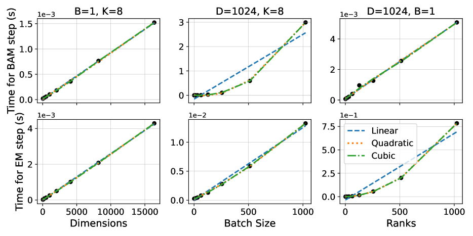
Figure 1: Scaling of pBaM algorithm with dimensions, batch size and rank. The top row shows the timing for BaM step (without evaluating the scores of the target) and the bottom row shows timing for a single EM step. All timings are in seconds.

Before proceeding to numerical experiments, we study the scaling of our algorithm with different components. Here we only show the empirical results, and a detailed discussion of these scalings is deferred to Appendix A.3. Every iteration of our approach consists of two steps—a BaM update and the patch step, which is implemented as series of EM updates. In Figure 1, we show the time taken for the BaM update and a single EM step for increasing dimensions ($D$), batch size ($B$) and ranks ($K$), varying each component while keeping others fixed. For the BaM step, we use a dummy model in which the time taken for evaluating scores is negligible.

There are two important takeaways from this figure. First, as desired, the scaling of both steps is linear with dimensions. The scaling of BaM step is linear with ranks and cubic with batch size, which is the same as BaM with full covariance. On the other hand, the scaling of EM steps is linear with batch size and cubic with ranks.

Second, though EM step seems more expensive than BaM step, EM step is independent of the target distribution. On the other hand, BaM step in practice will involve evaluating the score, i.e., the gradients of the target distributions. For any physical model of reasonable complexity, this will likely be more expensive than a single iteration of EM step.

4 Related work

Structured covariances have been considered in several variational inference algorithms. In particular, Miller et al. (2017) and Ong et al. (2018) propose using the Gaussian family with low rank plus diagonal structured covariances as a variational family in a BBVI algorithm based on reparameterization of the ELBO objective. Tomczak et al. (2020) study the use of low-rank plus diagonal Gaussians for variational inference in Bayesian neural networks.

Bhatia et al. (2022) study the problem of fitting a low-rank plus diagonal Gaussian to a target distribution; they show that when the target itself is Gaussian, gradient-based optimization of the (reverse) KL divergence results in a power iteration. However, their approach restricts the diagonal to be constant.

Many alternative types of structured variational families have also been proposed (Saul and Jordan, 1995; Hoffman and Blei, 2015; Tan and Nott, 2018; Ko et al., 2024). In terms of alternative covariance structures, Tan and Nott (2018) enforce sparsity in the precision matrix that captures conditional independence structures, and Ko et al. (2024) propose a structured covariance with block diagonal structure.

5 Experiments

The patched BaM algorithm (pBaM) is implemented in JAX (Bradbury et al., 2018), and publicly available on Github. We compare pBaM against factorized and low rank plus diagonal ADVI (ADVI-D and ADVI-LR respectively) (Miller et al., 2017; Ong et al., 2018), both of which can scale to high dimensions. For smaller dimensions, we will also compare against ADVI with full covariance (ADVI-F) and Batch-and-Match (BaM) with full covariance. Unless otherwise mentioned, all experiments are done with batch size $B=32$.

pBaM Setup:

We set the parameters of the patch step to default values of $\eta=1.2$ and tolerance $t=10^{-4}$. We experimented with different values and found the algorithm to be robust in broad parameter range of $1<\eta<1.5$ and $t<10^{-3}$. We initialize the learning rate parameter to $\lambda_{0}=1$ and schedule it over iterations as $\lambda_{t}=\lambda_{0}/(1+t)$.

ADVI Implementation:

Our implementation of all three cases of ADVI leverages automatic differentiation in JAX and uses the ADAM optimizer (Kingma and Ba, 2015) to minimize the reverse KL divergence. In all experiments, we run a grid of learning rate and only show the best results. We schedule the learning rate to decrease linearly to the smallest value of $10^{-5}$ over the course of iterations. We also experimented with other forms of scheduling, e.g., cosine scheduling, but did not find significant differences in them.

Factorized and multivariate normal distributions are implemented in Numpyro. We implement our own version of the Gaussian distribution with low-rank plus diagonal covariance matrix that efficiently generates samples and evaluates log-probability using the Woodbury matrix inversion identity without constructing the full covariance matrix.

5.1 Synthetic Gaussian targets

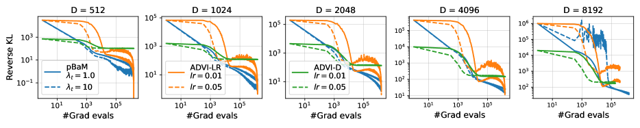
Figure 2: Performance with increasing dimensions for Gaussian with low-rank ($K=32$) plus diagonal covariance as target. We monitor reverse KL divergence for pBaM (blue) and ADVI-LR (orange) with $K=32$, and ADVI-D (green) for two different $\lambda_{t}$ and learning rate respectively (solid vs dashed).

We consider Gaussian target distributions with a low-rank plus diagonal covariance to study the performance of pBaM with dimensions and ranks:

$$p(z) =\mathcal{N}(z\,|\,\mu,\Psi+\Lambda\Lambda^{\top})$$

$$\mu\sim\mathcal{N}(0,1),\quad \Psi\sim\mathcal{U}(0,1),\quad\Lambda\sim\mathcal{N}(0,1),$$ (21)

where $\mu,\Psi\in\mathbb{R}^{D}$ and $\Lambda\in\mathbb{R}^{D\times K}$. Note that this distribution has strong off-diagonal components and the condition number $(\kappa)$ of this covariance matrix increases with increasing dimensions, e.g., $\kappa>10^{6}$ for $D>2048$ and $K=32$.

5.1.1 Performance with increasing dimensions

We begin by studying the performance of pBaM in the setting where the variational distribution and the target distribution are in the same family, and we show that despite the patch step, the algorithm converges to match the target, even in high dimensions.

Figure 2 shows the results on Gaussian targets with increasing dimensions, where we have fixed the rank $K=32$ for $\Lambda$. We show results for pBaM and ADVI-LR that fit this target distribution with variational approximations of the same rank, $K=32$. We monitor the reverse KL divergence as a function of gradient evaluations. Both algorithms are able to fit the target distribution, but pBaM converges much faster. We also show results for the best two learning rates for ADVI and two different values of $\lambda_{t}$ for pBaM. While the large learning rate of ADVI-LR converges faster initially, it gets stuck closer to the solution despite scheduling learning rate linearly. The performance of pBaM on the other hand is largely insensitive to $\lambda_{t}$, though $\lambda_{t}=1$ is more stable than $\lambda_{t}=10$ for $D=8192$.

5.1.2 Performance with increasing ranks

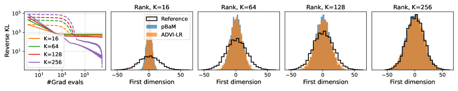
Figure 3: Performance with increasing ranks ($K$) for variational family. Target is 512 dimension Gaussian with low-rank ($K=256$) plus diagonal. We monitor reverse KL divergence for pBaM (solid) and ADVI-LR (dashed), and show marginal histograms for first dimension.

Next, we study the performance of pBaM with increasing ranks for the variational approximation. The results are in Figure 3. Here we have fixed the target to be low-rank plus Gaussian target (Eq. 21) with $D=512$ and $K=256$, and we fit it with variational distribution of ranks $K=16,64,128$ and $256$. In the last setting, the variational approximation and the target again belong to the same family, and expect an exact fit.

In the left panel of Figure 3, we again monitor the reverse KL divergence while the other panels show marginal histograms for the first dimension. Again, we find that while both ADVI-LR and pBaM converge to the same quality of solution, pBaM converges much faster. When the rank of the variational distribution is less than the target, the final approximation is more concentrated (smaller marginal variance). With increasing rank, the final approximation becomes a better fit, both in terms of reverse KL and capturing the variance of the target distribution.

5.2 Gaussian process inference

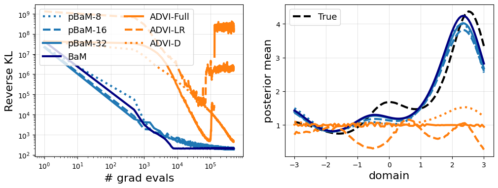
Figure 4: Synthetic GP-Poisson regression, $D=100$. We show the reverse KL (left) and the estimated rate using the posterior means (right).

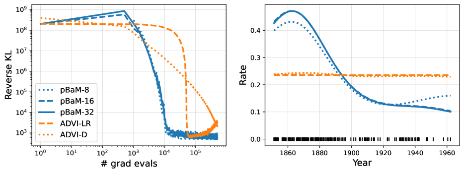
Figure 5: Log Gaussian Cox Process, $D=811$. We plot the reverse KL (left) and the estimated rate (right).

Consider a generative model of the form

$$f\sim\text{GP}(m,\tilde{\kappa}),\quad y_{1:N}|f \stackrel{{\scriptstyle iid}}{{\sim}}P_{f},$$ (22)

where $m$ is a mean function, $\tilde{\kappa}$ is a kernel function, and $P_{f}$ is a distribution that characterizes the likelihood of a data point. This structure describes many popular models with intractable posteriors, such as Gaussian process regression (with e.g., Poisson or Negative Binomial likelihoods), Gaussian process classification, and many spatial statistics models (e.g., the log-Gaussian Cox process).

The function $f$ is typically represented as a vector of function evaluations on a set of $D$ points, and thus can be itself high-dimensional (even if the data are low dimensional).

Poisson regression.

We consider a Poisson regression problem in $D=100$ dimensions, where

$$p(y_{1},\ldots,y_{N};f)=\prod_{n=1}^{N}\text{Pois}(y_{n};\lambda_{n}),\quad\lambda_{n}=\exp(f_{n}).$$

Data were generated from this model using a GP with mean function 0 and an RBF kernel with a lengthscale of 1.

In Figure 4, we compare pBaM with ranks $K=8,16,32$ against the BaM algorithm and ADVI (with full, rank 32, and diagonal covariances). In the left plot, we report the reverse KL vs the number of gradient evaluations. Here we observe that the low-rank BaM algorithms converge almost as quickly as the full-rank BaM algorithm. We found that even with extensive tuning of the learning rate, the ADVI algorithms tended to perform poorly for this model; the full covariance ADVI algorithm diverges. In the right plot, we show the true rate function along with the inferred rate functions (we report the posterior mean from the VI algorithms). For the BaM/pBaM methods, we found that increasing the rank results in a better fit.

Log-Gaussian Cox process.

Now we consider the log-Gaussian Cox process (LGCP) (Møller et al., 1998), which is used to model point process data. One approach to approximate the log-Gaussian Cox process is to bin the points, and to consider a Poisson likelihood for the counts in each bin. Specifically, we consider $p(y_{1},\ldots,y_{N};f)=\prod_{n=1}^{N}\text{Pois}(y_{n};\exp(f(x_{n})+m)$, where $m$ represents a mean offset.

We apply this model to a coal mining disasters data set (Carlin et al., 1992), which contains 191 events of mining explosions in Britain between March 15, 1851 and March 22, 1962. Following Murray et al. (2010), we bin the points into $811$ bins, and so the latent space is $D=811$ dimensional; in addition, we use an RBF kernel with a lengthscale of $37$ and set the mean to $m=\log(191/811)$.

The left panel of Figure 5 shows the results of pBaM on ranks $8,16,32$, ADVI-LR and ADVI-D. Here we report the reverse KL divergence, and pBaM converges much faster than the ADVI methods. Notably, the varying ranks for pBaM perform similarly. The right panel of Figure 5 shows the estimated rate functions using the posterior mean of the variational inference algorithms; the event data are visualized in the black rug plot points. Compared with MCMC sampled for this problem (e.g., Nguyen and Bonilla (2014, Figure 4)), the estimated intensity from pBaM is much more accurate than the ADVI solutions.

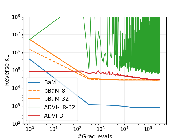
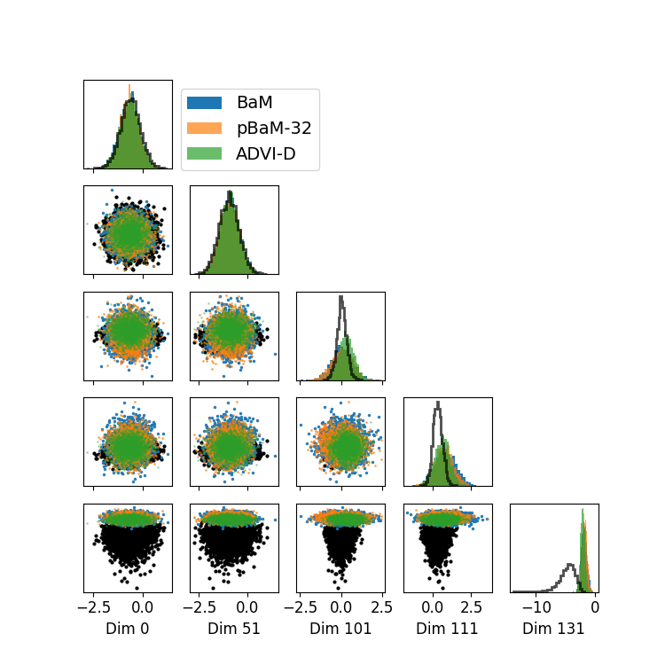
Figure 6: We show the reverse KL as well as 2-D marginals for five randomly selected dimensions for fitting IRT model with BaM, pBaM for ranks K=8 and 32, and ADVI-D. ADVI-LR and ADVI-F did not converge for this model.

5.3 IRT model

Given $I$ students and $J$ questions, item response theory (IRT) models how students answer questions on a test depending on student ability ($\alpha_{i}$), question difficulty ($\beta_{j}$), and the discriminatinative power of the questions ($\theta_{j}$) (Gelman and Hill, 2006). The observations given are the binary correctness $y_{ij}$ of $i$th student answer for question $j$. Both the mean-centered ability of the student $\alpha_{i}$, and the difficulty of questions $\beta_{j}$ have hierarchical priors. These terms are combined into something like a logistic regression with a multiplicative discrimination parameter.

We show the results for this model in Figure 6. Here $I=20$ and $J=100$, leading to dimensionality $D=143$. Despite tuning learning rates, ADVI-LR and ADVI-F diverged on this model. Full-rank BAM converges to a better reverse KL divergence than the low-rank pBaM or the factorized approximation of ADVI-D. However the two-dimensional marginals for pBaM look closer to BAM than the factorized approximation.

6 Discussion and future work

We have developed a score-based black-box variational inference algorithm for high-dimensional problems that fits a structured Gaussian variational family where the covariance can be represented as a sum of a low-rank and diagonal (LR+D) component. In particular, we extend the batch-and-match algorithm by adding a patch step that projects the dense covariance matrix to one that is structured. The computational and storage costs of this algorithm scale linearly in the dimension $D$. Empirically, we find that our algorithm converges faster than ADVI with LR+D, and is more stable on real world examples. We provide a Python implementation of pBaM at https://github.com/modichirag/GSM-VI/tree/dev.

A number of future directions remain. One direction is to study pBaM for a larger variety of high dimensional problems, particularly Bayesian neural networks. Another would be to adapt the algorithm to successively increase the rank of variational approximation (boosting) after an initial low-rank fit. Finally, we can also consider other structured covariances, e.g. sparse matrices, for scaling score-based VI to high dimensions.

Appendix A The patch step: additional details

A.1 Derivation of the patch step update

In this section, we derive the infinite-data-limit EM algorithm for factor analysis in the context of the setting considered here. In particular, we consider the model in Eq. 14 and the objective in Eq. 17.

Recall that $\tilde{q}_{t+\scriptscriptstyle\frac{1}{2}}(z)=\mathcal{N}(z\,|\,0,\Sigma_{t+\scriptscriptstyle\frac{1}{2}})$, where we assume we are given $\Sigma_{t+\scriptscriptstyle\frac{1}{2}}$ (as we discuss in Section 3.1, we do not need to form this matrix explicitly).

First note that the joint distribution under the model in Eq. 14 is

$$\begin{bmatrix}\zeta\\ z\end{bmatrix}\sim\mathcal{N}\left(\begin{bmatrix}0\\ 0\end{bmatrix},\begin{bmatrix}I&\Lambda^{\top}\\ \Lambda&\Lambda\Lambda^{\top}+\Psi\end{bmatrix}\right).$$ (A.1)

Defining $\beta~{}:=~{}\Lambda^{\top}(\Lambda\Lambda^{\top}+\Psi)^{-1}$, the conditional distribution of $\zeta|z,\Psi,\Lambda$ is Gaussian with mean and covariance

$$\mathbb{E}_{q}[\zeta\,|\,z] :=\Lambda^{\top}(\Lambda\Lambda^{\top}+\Psi)^{-1}z=\beta z$$ (A.2)

$$\text{Cov}_{q}[\zeta\,|\,z] :=I-\Lambda^{\top}(\Lambda\Lambda^{\top}+\Psi)^{-1}\Lambda=I-\beta\Lambda.$$ (A.3)

In what follows, we denote the conditional expectation with respect to $q(\zeta\,|\,z,\Lambda_{\tau},\Psi_{\tau})$ as $\mathbb{E}_{q}[\cdot]$, where $\tau$ represents the current EM iteration number. In the E-step, we compute the following statistics of the conditional distribution (Eq. A.2 and Eq. A.3) of the hidden variable $\zeta$ given $z$ and the current parameters $\Lambda_{\tau},\Psi_{\tau}$:

$$\mathbb{E}_{q}[\zeta] =\beta_{\tau}z$$ (A.4)

$$\mathbb{E}_{q}[\zeta\zeta^{\top}] =\mathbb{E}_{q}[\zeta]\mathbb{E}_{q}[\zeta]^{\top}+\text{Cov}_{q}[\zeta]=\beta_{\tau}zz^{\top}\beta_{\tau}^{\top}+I-\beta_{\tau}\Lambda_{\tau},$$ (A.5)

where $\beta_{\tau}:=\Lambda_{\tau}^{\top}(\Lambda_{\tau}\Lambda_{\tau}^{\top}+\Psi_{\tau})^{-1}$.

In the M-step, we maximize the objective in Eq. 17. First, we rewrite the objective in terms of the optimization variables $(\Lambda,\Psi)$ and constants. The log joint distribution is

$$\log q(\zeta,z) =-\tfrac{1}{2}(z-\Lambda\zeta)^{\top}\Psi^{-1}(z-\Lambda\zeta)-\tfrac{\log|\Psi|}{2}+\text{const.},$$

and so the objective is

$$\mathcal{L} :=\!-\mathbb{E}_{\tilde{q}_{t+\scriptscriptstyle\frac{1}{2}}}\!\left[\mathbb{E}_{q}\!\left[\log\!\left({q(\zeta,z\,|\,\Lambda,\Psi)}\!\right)\!\right]\right]+\text{const.},$$ (A.6)

$$=\tfrac{1}{2}\mathbb{E}_{\tilde{q}_{t+\scriptscriptstyle\frac{1}{2}}}\!\left[\mathbb{E}_{q}\!\left[z^{\top}\Psi^{-1}z-2z^{\top}\Psi^{-1}\Lambda\zeta+\zeta^{\top}\Lambda^{\top}\Psi^{-1}\Lambda\zeta\right]\right]+\tfrac{\log|\Psi|}{2}+\text{const.},$$ (A.7)

$$=\tfrac{1}{2}\mathbb{E}_{\tilde{q}_{t+\scriptscriptstyle\frac{1}{2}}}\!\left[z^{\top}\Psi^{-1}z\!-\!2z^{\top}\Psi^{-1}\Lambda\mathbb{E}_{q}[\zeta]\!+\!\text{tr}(\Lambda^{\top}\Psi^{-1}\Lambda\mathbb{E}_{q}[\zeta\zeta^{\top}])\right]+\tfrac{\log|\Psi|}{2}+\text{const.},$$ (A.8)

Assuming we can exchange limits (and thus derivatives) and integration, below, we compute the derivatives with respect to the optimization parameters. We will use the following identities (Petersen and Pedersen, 2008):

$$\nabla_{\mathcal{C}}a^{\top}\mathcal{C}b =ab^{\top}$$ (A.9)

$$\nabla_{\mathcal{C}}\text{tr}(\mathcal{C}A\mathcal{C}^{\top}) =2\mathcal{C}A$$ (A.10)

$$\nabla_{\mathcal{C}}\log(|\mathcal{C}|) =\mathcal{C}^{-1}$$ (A.11)

$$\nabla_{\mathcal{C}}\text{tr}\{\mathcal{C}B\} =B^{\top},$$ (A.12)

where we assume above that $A=A^{\top}$.

Derivative w.r.t. $\Lambda$.

Setting the derivative of Eq. A.8 with respect to $\Lambda$ to 0, i.e.,

$$\nabla_{\Lambda}\mathcal{L} =\mathbb{E}_{\tilde{q}_{t+\scriptscriptstyle\frac{1}{2}}}\left[\Psi^{-1}z\mathbb{E}_{q}[\zeta]^{\top}-\Psi^{-1}\Lambda\mathbb{E}[\zeta\zeta^{\top}]\right]=0,$$ (A.13)

implies that

$$\Lambda^{*} =\mathbb{E}_{\tilde{q}_{t+\scriptscriptstyle\frac{1}{2}}}[z\mathbb{E}_{q}[\zeta]^{\top}]\left(\mathbb{E}_{\tilde{q}_{t+\scriptscriptstyle\frac{1}{2}}}\mathbb{E}_{q}[\zeta\zeta^{\top}]\right)^{-1}$$ (A.14)

$$=\mathbb{E}_{\tilde{q}_{t+\scriptscriptstyle\frac{1}{2}}}[zz^{\top}]\beta_{\tau}^{\top}(\beta_{\tau}\mathbb{E}_{\tilde{q}_{t+\scriptscriptstyle\frac{1}{2}}}[zz^{\top}]\beta_{\tau}^{\top}+I-\beta_{\tau}\Lambda_{\tau})^{-1}$$ (A.15)

$$=\Sigma_{t+\scriptscriptstyle\frac{1}{2}}\beta_{\tau}^{\top}(\beta_{\tau}\Sigma_{t+\scriptscriptstyle\frac{1}{2}}\beta_{\tau}^{\top}+I-\beta_{\tau}\Lambda_{\tau})^{-1},$$ (A.16)

where in the second line we plugged in the statistics from Eq. A.4 (note that the statistics are evaluated with respect to the current parameters $\Lambda_{\tau},\Psi_{\tau}$), and in the third line we used $\mathbb{E}_{\tilde{q}_{t+\scriptscriptstyle\frac{1}{2}}}[zz^{\top}]=\Sigma_{t+\scriptscriptstyle\frac{1}{2}}$.

Derivative w.r.t. $\Psi$.

Taking the derivative w.r.t. $\Psi^{-1}$ and setting $\nabla_{\Psi^{-1}}\mathcal{L}=0$, i.e.,

$$\tfrac{1}{2}\mathbb{E}_{\tilde{q}_{t+\scriptscriptstyle\frac{1}{2}}}\left[zz^{\top}\!\!-\!2\Lambda\mathbb{E}_{q}[\zeta]z^{\top}\!+\!\Lambda\mathbb{E}_{q}[\zeta\zeta^{\top}]\Lambda^{\top}\right]-\tfrac{1}{2}\Psi=0$$ (A.17)

results in

$$\Psi^{*} =\mathbb{E}_{\tilde{q}_{t+\scriptscriptstyle\frac{1}{2}}}\left[zz^{\top}-2\Lambda\mathbb{E}_{q}[\zeta]z^{\top}+\Lambda\mathbb{E}_{q}[\zeta\zeta^{\top}]\Lambda^{\top}\right]$$ (A.18)

$$=\mathbb{E}_{\tilde{q}_{t+\scriptscriptstyle\frac{1}{2}}}[zz^{\top}]-\Lambda\mathbb{E}_{\tilde{q}_{t+\scriptscriptstyle\frac{1}{2}}}[\mathbb{E}_{q}[\zeta]z^{\top}]$$ (A.19)

$$=\Sigma_{t+\scriptscriptstyle\frac{1}{2}}-\Lambda\beta_{\tau}\Sigma_{t+\scriptscriptstyle\frac{1}{2}}$$ (A.20)

$$=(I-\Lambda\beta_{\tau})\Sigma_{t+\scriptscriptstyle\frac{1}{2}},$$ (A.21)

where the second line follows from substituting the $\Lambda^{*}$ update into the third term of Eq. A.18.

The final update results from taking the diagonal part of $\Psi^{*}$ above. Note that this update depends on the newly updated $\Lambda^{*}$ term in Eq. A.18 (as opposed to the current $\Lambda_{\tau}$).

A.2 The path step updates monotonically improve KL divergence

Suppose we have an auxiliary function that has the following properties:

1. $\mathcal{A}(\theta,\theta)=\text{KL}(\tilde{q}_{t+\scriptscriptstyle\frac{1}{2}},q_{\theta})$

2. $\mathcal{A}(\theta,\theta^{\prime})\geq\text{KL}(\tilde{q}_{t+\scriptscriptstyle\frac{1}{2}},q_{\theta^{\prime}})$ for all $\theta^{\prime}\in\Theta$.

Then the update

$$\theta_{\tau+1}=\arg\min_{\theta\in\Theta}\mathcal{A}(\theta_{\tau},\theta)$$ (A.22)

monotonically decreases $\text{KL}(\tilde{q}_{t+\scriptscriptstyle\frac{1}{2}};q)$ at each iteration. The property that the KL divergence monotonically decreases holds because

$$\text{KL}(\tilde{q}_{t+\scriptscriptstyle\frac{1}{2}},q_{\theta_{\tau}}) =\mathcal{A}(\theta_{\tau},\theta_{\tau})$$ (A.23)

$$\geq\mathcal{A}(\theta_{\tau},\theta_{\tau+1})$$ (A.24)

$$\geq\text{KL}(\tilde{q}_{t+\scriptscriptstyle\frac{1}{2}},q_{\theta_{\tau+1}}),$$ (A.25)

where Eq. A.23 is due to Property 1, Eq. A.24 is by construction from the update, and Eq. A.25 is due to Property 2.

We now show that an auxiliary function satisfying Property 1 and 2 above exists. In particular, consider

$$\mathcal{A}(\theta,\theta^{\prime}) =\mathbb{E}_{\tilde{q}_{t+\scriptscriptstyle\frac{1}{2}}}\!\left[\log\tilde{q}_{t+\scriptscriptstyle\frac{1}{2}}(z)\!-\!\!\int\!\log\!\left(\tfrac{q(\zeta,z\,|\,\theta^{\prime})}{q(\zeta\,|\,z,\theta)}\!\right)\!q(\zeta\,|\,z,\theta)d\zeta\right],$$ (A.26)

where $q(\zeta\,|\,z,\theta)\propto q(\zeta)q(z\,|\,\zeta,\theta)$ is the conditional distribution of the hidden variable induced by Eq. 14.

If $\theta^{\prime}=\theta$, then Property 1 is satisfied: since $\log\frac{q(\zeta,z\,|\,\theta)}{q(\zeta\,|\,z,\theta)}=\log q_{\theta}(z)$ and $\int q(\zeta\,|\,z)dz=1$, this results in $\mathcal{A}(\theta,\theta)=\text{KL}(\tilde{q}_{t+\scriptscriptstyle\frac{1}{2}},q_{\theta})$.

Property 2 can be verified using an application of Jensen’s inequality to the second term of Eq. A.26:

$$\mathcal{A}(\theta,\theta^{\prime}) \geq\mathbb{E}_{\tilde{q}_{t+\scriptscriptstyle\frac{1}{2}}}\!\left[\log\tilde{q}_{t+\scriptscriptstyle\frac{1}{2}}(z)\!-\!\log\!\int\!\!\left(\tfrac{q(\zeta,z\,|\,\theta^{\prime})}{q(\zeta\,|\,z,\theta)}\!\right)\!q(\zeta|z,\theta)d\zeta\right]$$

$$=\mathbb{E}_{\tilde{q}_{t+\scriptscriptstyle\frac{1}{2}}}\!\left[\log\tilde{q}_{t+\scriptscriptstyle\frac{1}{2}}(z)\!-\!\log\!\int\!\!{q(\zeta,z\,|\,\theta^{\prime})}d\zeta\right]$$

$$=\text{KL}(\tilde{q}_{t+\scriptscriptstyle\frac{1}{2}},q_{\theta^{\prime}}).$$

Thus, minimizing the function in Eq. A.26 monotonically decreases the KL divergence.

Summary of objective and updates.

Combining Eq. A.22 and Eq. A.26 results in the iteration in Eq. 17: i.e.,

$$\theta_{\tau+1}\!=\!\arg\min_{\theta\in\Theta}\mathbb{E}_{\tilde{q}_{t+\scriptscriptstyle\frac{1}{2}}}\!\left[\!-\!\!\!\int\!\log({q(\zeta,z\,|\,\theta)})q(\zeta\,|\,z,\theta_{\tau})d\zeta\right]\!\!+\!\text{const.},$$ (A.27)

where the constant represents factors that are independent of $\theta$.

A.3 Computational cost of BaM update and the patch step

We first show that the computational cost of the BaM update with a structured covariance is linear in the dimension $D$. Next we discuss the computational cost of the patch step, which in combination with the BaM update, results in a computational cost linear in $D$.

Recall from Eq. 12 that the covariance can be written as

$$\Sigma_{t+\scriptscriptstyle\frac{1}{2}} =\Psi_{t}+R_{t}R_{t}^{\top}-(\Psi_{t}+R_{t}R_{t}^{\top})^{\top}Q_{t}M_{t}Q_{t}^{\top}(\Psi_{t}\!+\!R_{t}R_{t}^{\top}),$$

where $Q_{t}~{}\in~{}\mathbb{R}^{D\times(B+1)}$ and $R_{t}~{}\in~{}\mathbb{R}^{D\times(K+B+1)}$, and $\Psi_{t}$ is a $D$-dimensional diagonal matrix.

First consider $H_{t}:=(\Psi_{t}+R_{t}R_{t}^{\top})^{\top}Q_{t}$, where $H_{t}\in\mathbb{R}^{D\times(B+1)}$; this matrix can be constructed with $\mathcal{O}((K+B)BD)$ computation.

Then we store $\Sigma_{t+\scriptscriptstyle\frac{1}{2}}$ implicitly by storing the matrices $\Psi_{t},\,R_{t},H_{t}$ and $M_{t}$:

$$\Sigma_{t+\scriptscriptstyle\frac{1}{2}} =\Psi_{t}+R_{t}R_{t}^{\top}-H_{t}M_{t}H_{t}^{\top},$$ (A.28)

Note that evaluating $R_{t}R_{t}^{\top}$ can be a $\mathcal{O}(D^{2})$ operation, but since we store $R_{t}$, we do not need to explicitly evaluate it now, and we will be able to contract it with other elements in the patch update to maintain $\mathcal{O}(D)$ computation.

The matrix $M_{t}\in~{}\mathbb{R}^{(B+1)\times(B+1)}$ defined in the update is:

$$M_{t}:=\big{[}\tfrac{1}{2}I_{B+1}\!+\!\left(Q_{t}^{\top}(\Psi_{t}+R_{t}R_{t}^{\top})Q_{t}+\tfrac{1}{4}I_{B+1}\right)^{\frac{1}{2}}\big{]}^{-2}=\big{[}\tfrac{1}{2}I_{B+1}\!+\!\left(H_{t}^{\top}Q_{t}+\tfrac{1}{4}I_{B+1}\right)^{\frac{1}{2}}\big{]}^{-2}.$$

Here evaluating the matrix in the square-root takes $\mathcal{O}(DB^{2})$ computation, and it takes $\mathcal{O}(B^{3})$ to compute the square root of and the inverse of the matrix. Thus, overall, the total computational cost of BaM update is $\mathcal{O}(DB^{2}+B^{3}+KBD)$; that is, it is linear in $D$.

Next, we turn to the computational cost of the patch step. Every iteration of patch step requires us to compute:

$$\beta_{\tau} =\Lambda_{\tau}^{\top}\Psi_{\tau}^{-1}[I_{K}\!-\!\Lambda_{\tau}(I+\Lambda_{\tau}^{\top}\Psi_{\tau}^{-1}\Lambda_{\tau})^{-1}\Lambda_{\tau}^{\top}\Psi_{\tau}^{-1}]\quad\text{(via~{}Woodbury~{}inverse~{}identity)}$$

$$\Lambda_{\tau+1} =\Sigma_{t+\scriptscriptstyle\frac{1}{2}}\beta_{\tau}^{\top}(\beta_{\tau}\Sigma_{t+\scriptscriptstyle\frac{1}{2}}\beta_{\tau}^{\top}+I_{K}-\beta_{\tau}\Lambda_{\tau})^{-1},$$

$$\Psi_{\tau+1} =\mathrm{diag}((I_{D}-\Lambda_{\tau+1}\beta_{\tau})\Sigma_{t+\scriptscriptstyle\frac{1}{2}})$$

Here $\beta_{\tau}\in\mathbb{R}^{K\times D}$, and evaluating $\beta_{\tau}$ requires forming matrix products that take $\mathcal{O}(K^{2}D$) computation and inverting a $K\times K$ matrix, which in total takes $\mathcal{O}(K^{2}D+K^{3})$ computation.

Using Eq. A.28, $\Sigma_{t+\scriptscriptstyle\frac{1}{2}}\beta_{\tau}^{\top}$ can be evaluated in $\mathcal{O}(DK(K+B))$, and hence the $\Lambda_{\tau}$ update can be evaluated in $\mathcal{O}(DK(K+B)+K^{3})$ computation, with a similar complexity for $\Psi$ update.

Appendix B Additional experiments

In Table B.1, we provide an overview of the problems studied in this paper.

Table B.1: Summary of problems

Problem	Target	$D$
Synthetic	Gaussian	512
Synthetic	Gaussian	1024
Synthetic	Gaussian	2048
Synthetic	Gaussian	4096
Synthetic	Gaussian	8192
Poisson regression	Non-Gaussian	100
Log Gaussian Cox process	Non-Gaussian	811
IRT model	Non-Gaussian	143

B.1 Impact of hyperparameters on Gaussian example

Here we show the impact of varying choices of parameters like scheduling, learning rate, and batch size for ADVI-LR and pBaM on the synthetic Gaussian example. We always work in the setting where the rank of the low-rank component of the target and the variational distribution is the same ($K=32$).

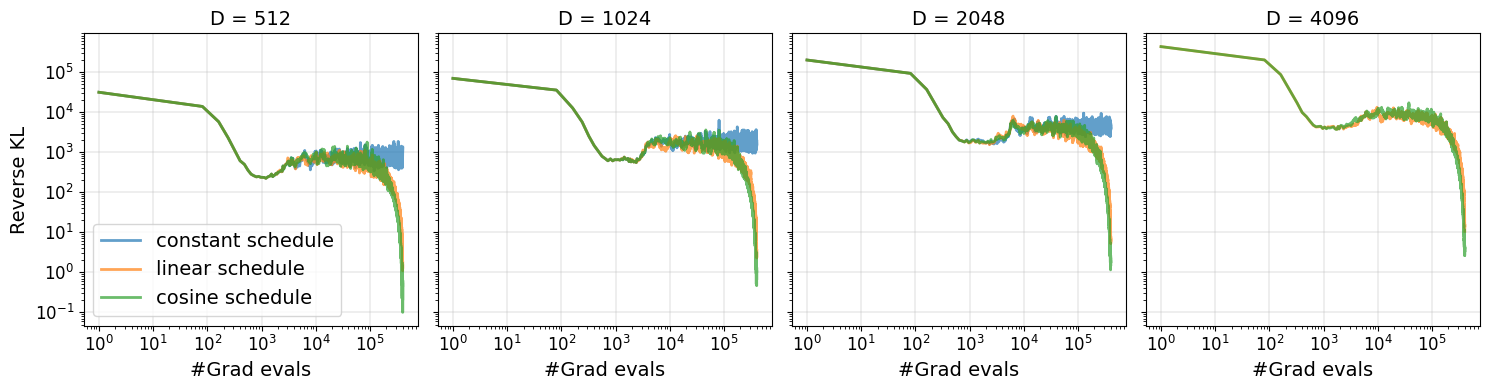
Figure B.1: Impact of scheduling the learning rate for ADVI-LR.

Figure B.1 shows the impact of scheduling the learning rate. We consider no scheduling (constant learning rate), linear and cosine scheduling. We fix the inital and final learning rate to be $0.1$ and $10^{-5}$ respectively, and batch size $B=8$. All three schedules converge at the same rate initially, however the constant learning rate asymptotes at a higher loss (KL divergence) once it reaches closer to the solution. Both linear and cosine scheduling give similar performance. Hence we use linear scheduling for all experiments.

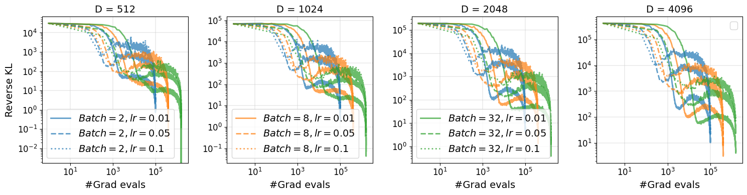
Figure B.2: Impact of changing the batch size and the learning rate for ADVI-LR.

Next in Figure B.2, we study the impact of learning rate and batch size. Broadly, we find that the higher learning rate converges more quickly initially, but plateaus to a larger loss before decreasing sharply again. Smaller batch sizes show faster convergence initially, while they plateau at a lower KL divergence. Hence we use batch size $B=32$ for all the experiments. However, the conclusion of this figure along with Figure B.1 suggests that the relationship with learning rate is more complicated. Given that pBaM seems to outperform all these learning rates considered nevertheless, we show results for two best learning rates in the main text.

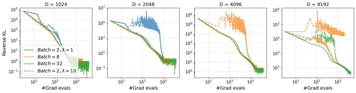
Figure B.3: Impact of changing the batch size and the learning rate parameter $\lambda_{t}$ for pBaM.

Finally we study the impact of batch size and learning rate parameter $\lambda_{t}$ for pBaM in Figure B.3. Overall, the algorithm seems to get increasingly more stable for larger batch size, and smaller $\lambda_{t}$ for a given batch size. However the convergence rate for any stable run seems to broadly be insensitive to these choices.

B.2 Gaussian process inference

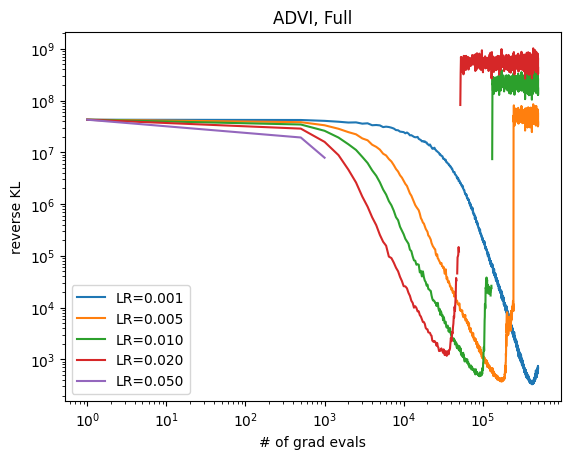
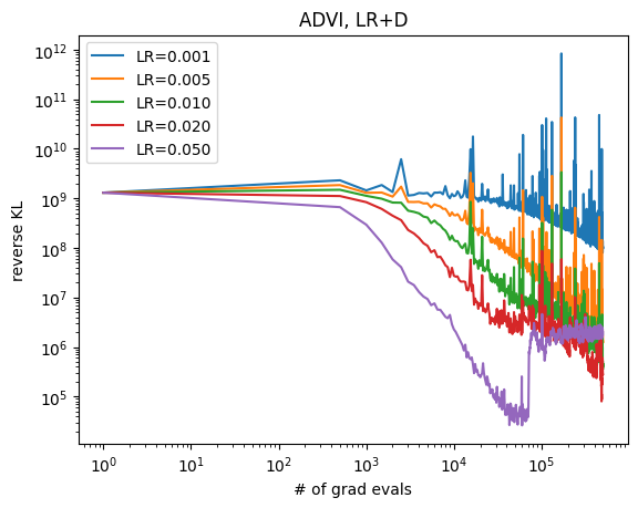
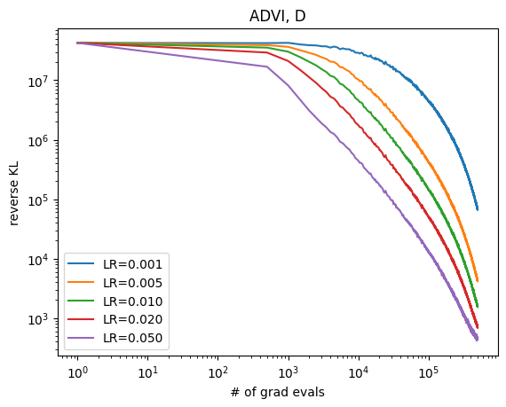
Figure B.4: Poisson regression $D=100$ with varying learning rates for ADVI

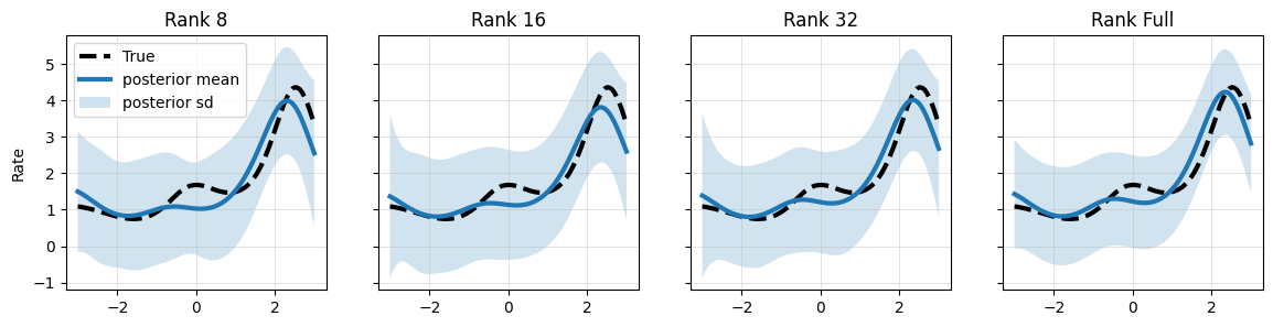
Figure B.5: Poisson regression $D=100$. BaM/pBaM with varying ranks.

B.2.1 Poisson regression

In Section 5, we studied a $D=100$ Poisson regression problem. First, we show in Figure B.4 the results of the different ADVI methods on a range of learning rates: $0.001,0.005,0.01,0.02,0.05$. For the final plots, the learning rate was set to 0.02. For the full covariance family, we also tried a linear schedule and found similar results. We also found larger batch sizes to be more stable, and so in all plots for this example, we set $B=50$. In Figure B.5 we visualize the results of BaM/pBaM for varying ranks; the estimated mean rates in the right panel of Figure 4, but here we additionally show the uncertainties estimated from the posterior standard deviations.

B.2.2 Log Gaussian Cox process

In this example, the dimension was 811, and so we only ran the variational inference methods with diagonal and low-rank plus diagonal families. We show in Figure B.6 ADVI for these families, varying the learning rate on a grid. In Figure B.7, we show the BaM/pBaM estimated mean rate and uncertainty computed using the variational posterior mean and standard deviation. Overall, the differences in this set of ranks were small.

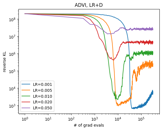
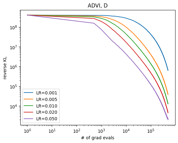
Figure B.6: LGCP, $D=811$. ADVI with varying learning rate.

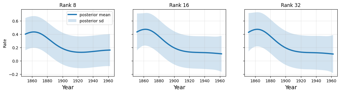
Figure B.7: LGCP, $D=811$. BaM/pBaM with varying ranks.

References

- Bhatia et al. (2022) K. Bhatia, N. L. Kuang, Y.-A. Ma, and Y. Wang. Statistical and computational trade-offs in variational inference: A case study in inferential model selection. arXiv eprint 2207.11208, 2022.
- Blei et al. (2017) D. M. Blei, A. Kucukelbir, and J. D. McAuliffe. Variational inference: A review for statisticians. Journal of the American Statistical Association, 112(518):859–877, 2017.
- Bradbury et al. (2018) J. Bradbury, R. Frostig, P. Hawkins, M. J. Johnson, C. Leary, D. Maclaurin, G. Necula, A. Paszke, J. VanderPlas, S. Wanderman-Milne, and Q. Zhang. JAX: composable transformations of Python+NumPy programs, 2018.
- Cai et al. (2024a) D. Cai, C. Modi, C. Margossian, R. Gower, D. Blei, and L. Saul. EigenVI: score-based variational inference with orthogonal function expansions. In Advances in Neural Information Processing Systems, to appear, 2024a.
- Cai et al. (2024b) D. Cai, C. Modi, L. Pillaud-Vivien, C. Margossian, R. Gower, D. Blei, and L. Saul. Batch and match: black-box variational inference with a score-based divergence. In International Conference on Machine Learning, 2024b.
- Carlin et al. (1992) B. P. Carlin, A. E. Gelfand, and A. F. Smith. Hierarchical Bayesian analysis of changepoint problems. Journal of the Royal Statistical Society: Series C (Applied Statistics), 41(2):389–405, 1992.
- Gelman and Hill (2006) A. Gelman and J. Hill. Data analysis using regression and multilevel/hierarchical models. Cambridge University Press, 2006.
- Ghahramani and Hinton (1996) Z. Ghahramani and G. E. Hinton. The EM algorithm for mixtures of factor analyzers. Technical report, Technical Report CRG-TR-96-1, University of Toronto, 1996.
- Hoffman and Blei (2015) M. D. Hoffman and D. M. Blei. Structured stochastic variational inference. In Artificial Intelligence and Statistics, pages 361–369, 2015.
- Jordan et al. (1999) M. I. Jordan, Z. Ghahramani, T. S. Jaakkola, and L. K. Saul. An introduction to variational methods for graphical models. Machine Learning, 37:183–233, 1999.
- Kingma and Ba (2015) D. P. Kingma and J. Ba. Adam: A method for stochastic optimization. In International Conference on Learning Representations, 2015.
- Kingma and Welling (2014) D. P. Kingma and M. Welling. Auto-encoding variational Bayes. In International Conference on Learning Representations, 2014.
- Ko et al. (2024) J. Ko, K. Kim, W. C. Kim, and J. R. Gardner. Provably scalable black-box variational inference with structured variational families. In International Conference on Machine Learning, 2024.
- Kucukelbir et al. (2017) A. Kucukelbir, D. Tran, R. Ranganath, A. Gelman, and D. M. Blei. Automatic differentiation variational inference. Journal of Machine Learning Research, 2017.
- Miller et al. (2017) A. C. Miller, N. J. Foti, and R. P. Adams. Variational boosting: Iteratively refining posterior approximations. In International Conference on Machine Learning, pages 2420–2429. PMLR, 2017.
- Modi et al. (2023) C. Modi, C. Margossian, Y. Yao, R. Gower, D. Blei, and L. Saul. Variational inference with Gaussian score matching. Advances in Neural Information Processing Systems, 36, 2023.
- Møller et al. (1998) J. Møller, A. R. Syversveen, and R. P. Waagepetersen. Log Gaussian Cox processes. Scandinavian Journal of Statistics, 25(3):451–482, 1998.
- Murray et al. (2010) I. Murray, R. Adams, and D. MacKay. Elliptical slice sampling. In Artificial Intelligence and Statistics, volume 9, pages 541–548, 2010.
- Nguyen and Bonilla (2014) T. V. Nguyen and E. V. Bonilla. Automated variational inference for Gaussian process models. Advances in Neural Information Processing Systems, 27, 2014.
- Ong et al. (2018) V. M.-H. Ong, D. J. Nott, and M. S. Smith. Gaussian variational approximation with a factor covariance structure. Journal of Computational and Graphical Statistics, 27(3):465–478, 2018.
- Petersen and Pedersen (2008) K. B. Petersen and M. S. Pedersen. The matrix cookbook. Technical University of Denmark, 7(15):510, 2008.
- Ranganath et al. (2014) R. Ranganath, S. Gerrish, and D. Blei. Black box variational inference. In Artificial Intelligence and Statistics, pages 814–822. PMLR, 2014.
- Rubin and Thayer (1982) D. B. Rubin and D. T. Thayer. EM algorithms for ML factor analysis. Psychometrika, 47:69–76, 1982.
- Saul and Jordan (1995) L. Saul and M. Jordan. Exploiting tractable substructures in intractable networks. Advances in Neural Information processing Systems, 8, 1995.
- Saul and Rahim (2000) L. K. Saul and M. G. Rahim. Maximum likelihood and minimum classification error factor analysis for automatic speech recognition. IEEE Transactions on Speech and Audio Processing, 8(2):115–125, 2000.
- Tan and Nott (2018) L. S. Tan and D. J. Nott. Gaussian variational approximation with sparse precision matrices. Statistics and Computing, 28:259–275, 2018.
- Titsias and Lázaro-Gredilla (2014) M. Titsias and M. Lázaro-Gredilla. Doubly stochastic variational Bayes for non-conjugate inference. In International Conference on Machine Learning. PMLR, 2014.
- Tomczak et al. (2020) M. Tomczak, S. Swaroop, and R. Turner. Efficient low rank Gaussian variational inference for neural networks. Advances in Neural Information Processing Systems, 33:4610–4622, 2020.
- Wainwright et al. (2008) M. J. Wainwright, M. I. Jordan, et al. Graphical models, exponential families, and variational inference. Foundations and Trends® in Machine Learning, 1(1–2):1–305, 2008.
- Yang et al. (2019) Y. Yang, R. Martin, and H. Bondell. Variational approximations using Fisher divergence. arXiv preprint arXiv:1905.05284, 2019.
- Zhang et al. (2018) C. Zhang, B. Shahbaba, and H. Zhao. Variational Hamiltonian Monte Carlo via score matching. Bayesian Analysis, 13(2):485, 2018.