Piecewise geodesic Jordan curves II: Loewner energy, projective structures, and accessory parameters

Abstract

Consider a Jordan curve on the Riemann sphere passing through $n\geq 3$ given points. We show that in each relative isotopy class of such curves, there exists a unique curve that minimizes the Loewner energy. These curves have the property that each arc between two consecutive points is a hyperbolic geodesic in the domain bounded by the other arcs. This geodesic property lets us define a complex projective structure on the punctured sphere. We show that its associated quadratic differential has simple poles, whose residues (accessory parameters) are given by the Wirtinger derivatives of the minimal Loewner energy, a result resembling Polyakov’s conjecture for the Fuchsian projective structure that was later proven by Takhtajan and Zograf. Finally, we show that the projective structures we obtain are related to the Fuchsian projective structures via a $\pi$-grafting.

1 Introduction

Let $n\geq 3$ be an integer. We call a Jordan curve $\gamma$ on the Riemann sphere $\widehat{\mathbb{C}}=\mathbb{C}\cup\{\infty\}$ through distinct points $z_{1},...,z_{n}$ piecewise geodesic if $\gamma\smallsetminus\{z_{1},...,z_{n}\}=\gamma_{1}\cup\gamma_{2}\cup\ldots\cup\gamma_{n}$ where $\gamma_{j}$ is a hyperbolic geodesic in $\widehat{\mathbb{C}}\smallsetminus(\gamma\smallsetminus\gamma_{j})$ for all $j=1,\ldots,n$. This class of Jordan curves was introduced and investigated from geometric function theoretic viewpoints in [12] (see also [23, 17, 15, 2]). Specifically, the conformal welding of these curves was characterized, the role of smoothness was elucidated, and explicit conformal maps were computed.

In the present paper, which is mostly self-contained, we investigate these curves from the Loewner theory perspectives and their relation to (complex) projective structures on the $n$-punctured sphere. Throughout this article, we call a function or a Jordan curve smooth if it is once continuously differentiable. Smooth piecewise geodesic curves arise naturally as minimizers of a certain functional related to Loewner theory, namely Loewner energy (see also [14, 26] for closely related energy minimizing problems). In Section 2, we review the basic properties of Loewner energy and show (Lemma 2.15) that every relative isotopy class of curves through points $z_{1},...,z_{n}$ contains at least one Loewner energy minimizer. Furthermore, each minimizer is piecewise geodesic. We also describe in Section 2.1 that these isotopy classes are in bijection with the Teichmüller space $T_{0,n}$ of the $n$-punctured sphere.

The first main result (Theorem 3.1) of this paper is the uniqueness of the smooth piecewise geodesic curve in its relative isotopy class. Hence, the unique smooth piecewise geodesic curve coincides with the energy minimizer. The proof relies on potential theory and does not refer to the Loewner theory. In other words, we obtain a parametrization of $T_{0,n}$ by the family of smooth piecewise geodesic Jordan curves. The welding homeomorphism associated with a Jordan curve is a homeomorphism of $\widehat{\mathbb{R}}=\mathbb{R}\cup\{\infty\}$. It was known that the welding homeomorphisms of piecewise geodesic curves are precisely the piecewise Möbius weldings (see [12] and Section 2.4), hence Theorem 3.1 also yields a simple parametrization of $T_{0,n}$ by smooth piecewise Möbius weldings as described in Section 4. Theorem 4.4, the main result of Section 4, shows that this parametrization provides a diffeomorphism between the space of smooth piecewise Möbius maps and $T_{0,n}$.

In Section 5, we associate a projective structure $Z_{\gamma}$ on the punctured sphere with each piecewise geodesic curve $\gamma$. The projective charts are given by the uniformizing conformal maps in the complement of the curve, which can be extended across each arc $\gamma_{j}$ thanks to the piecewise geodesic property. Theorem 3.1 then implies that we obtain a well-defined section of projective structures over the Teichmüller space $T_{0,n}$ given by the unique smooth piecewise geodesic curve in each relative isotopy class.

Furthermore, we observe that the holonomy of $Z_{\gamma}$ around each puncture is parabolic (Theorem 5.3) and that the quadratic differential comparing $Z_{\gamma}$ to the trivial projective structure has simple poles. The main result of Section 5 is Theorem 5.10, identifying the residues of the poles at the punctures $z_{k}$ as the Wirtinger derivatives $\partial_{z_{k}}$ of the Loewner energy of the smooth piecewise geodesic curve through the punctures. This result is very similar to the relation between the accessory parameters of the Fuchsian projective structure and the classical Liouville action, first conjectured by Polyakov and proved by Takhtajan and Zograf in [28, Thm. 1]. Our proof relies on the explicit computation of the conformal map of geodesic pairs from [12] (recalled in Section 2.5) and the differentiability results of Section 4.

The final Section 6 studies the relation between the Fuchsian projective structures on an $n$-punctured sphere and the projective structures $Z_{\gamma}$ described above. We show that they are related by a $\pi$-angle grafting along a hyperbolic geodesic in the $n$-punctured sphere (Proposition 6.2). Using the results above, we obtain that the $\pi$-angle grafting induces a diffeomorphism of $T_{0,n}$ (Corollary 6.3), which confirms the grafting conjecture for an $n$-punctured sphere in a special case. We also mention [18, 13] for the proof of the grafting conjecture for compact surfaces and general measured laminations.

2 Preliminaries

2.1 Teichmüller space of the $n$-punctured sphere

Recall that two Jordan curves $\gamma_{0},\gamma_{1}$ are isotopic relatively to $z_{1},...,z_{n}\in\widehat{\mathbb{C}}$ if there is a continuous family of Jordan curves $\gamma_{t}$ through $z_{1},...,z_{n}$ beginning with $\gamma_{0}$ and ending with $\gamma_{1}.$ We write $\mathcal{L}(z_{1},\ldots,z_{n};\gamma)$ for the isotopy class of Jordan curves containing (a representative curve) $\gamma$ which goes through $z_{1},\ldots,z_{n}$ in this order.

In Section 2.4 we will show that each isotopy class of curves contains a minimizer of the Loewner energy, and in the following section that the minimizer is unique. In the present section, we briefly discuss the role of the Teichmüller space $T_{0,n}$ of the $n-$punctured sphere as the natural domain of definition of the function that gives the minimal energy of Jordan curves through a prescribed set of $n$ points. To this end, we will describe how each isotopy class of Jordan curves through $n$ given points can be viewed as a point in $T_{0,n}$.

To fix a definition of $T_{0,n}$, we fix the base Riemann surface

$$\Sigma_{0}=\widehat{\mathbb{C}}\smallsetminus\{-(n-3),\ldots,-2,-1,0,1,\infty\}$$

and think of the extended real line $\widehat{\mathbb{R}}$ as a Jordan curve on the sphere through the $n$ punctures $-(n-3),-(n-2),\ldots,1,\infty$ of $\Sigma_{0}.$ A marked $n$-punctured sphere is a pair $(\Sigma,f)$ where $\Sigma=\widehat{\mathbb{C}}\smallsetminus\{z_{1},\ldots,z_{n-3},0,1,\infty\}$ and $f:\Sigma_{0}\to\Sigma$ a quasiconformal homeomorphism sending punctures to punctures (more precisely, sending $-(n-3)$ to $z_{1}$,…, and $0,1,\infty$ to $0,1,\infty$ in this order). Two marked surfaces $(\Sigma_{1},f_{1})$ and $(\Sigma_{2},f_{2})$ are equivalent if the quasiconformal homeomorphism $f_{2}\circ f_{1}^{-1}:\Sigma_{1}\to\Sigma_{2}$ is isotopic to a conformal map while fixing the marked points, hence isotopic to the identity map. Then $T_{0,n}$ is the set of equivalence classes of marked $n$-punctured spheres.

Now we turn the attention to Jordan curves passing through $n$ points $z_{1},...,z_{n}$ in this order. By composing with the Möbius transformation that sends $z_{n-2},z_{n-1}$ and $z_{n}$ to $0,1,\infty$, we may restrict our attention to Jordan curves $\gamma$ passing through points $z_{1},...,z_{n-3},0,1,\infty$ (in this order). As will become clear later, we are only interested in quasicircles, slightly simplifying the following presentation. Given a quasicircle $\gamma$ through $z_{1},...,z_{n-3},0,1,\infty,$ there is a quasiconformal homeomorphism $\phi$ of $\widehat{\mathbb{C}}$ mapping $\widehat{\mathbb{R}}$ to $\gamma$ and $-(n-3),\ldots,-2,-1,0,1,\infty$ to $z_{1},...,z_{n-3},0,1,\infty$ (in this order). Any two such quasiconformal maps $\phi_{1},\phi_{2}$ are isotopic, and we therefore obtain a map

$$F:\{((z_{1},...,z_{n-3},0,1,\infty),\gamma)\}\to T_{0,n}$$

by setting $F((z_{1},...,z_{n-3},0,1,\infty),\gamma)=(\Sigma,\phi)$ with $\Sigma=\widehat{\mathbb{C}}\smallsetminus\{z_{1},...,z_{n-3},0,1,\infty\}.$ Furthermore, if $\gamma_{1}$ and $\gamma_{2}$ are isotopic quasicircles through the same set of points, and if $\phi_{1}$ and $\phi_{2}$ are quasiconformal homeomorphisms mapping $\widehat{\mathbb{R}}$ to $\gamma_{1}$ and $\gamma_{2}$ as above, then $\phi_{1}$ and $\phi_{2}$ are again isotopic so that the map $F$ descends to the desired map from the set of isotopy classes $\{\mathcal{L}(z_{1},...,z_{n-3},0,1,\infty;\gamma)\}$ to $T_{0,n}$.

Conversely, every point of $T_{0,n}$ is represented by some quasiconformal map $f:\Sigma_{0}\to\widehat{\mathbb{C}}\smallsetminus\{z_{1},...,z_{n-3},0,1,\infty\}$ fixing $0,1,\infty$, and the points $z_{1},...,z_{n-3}$ are independent of the choice of the representative $f$. Moreover, the isotopy class of the Jordan curve $f(\widehat{\mathbb{R}})$ is independent of $f$, so that every point of $T_{0,n}$ corresponds to a unique point $\mathcal{L}(z_{1},...,z_{n-3},0,1,\infty;\gamma)$. We summarize our discussion as follows.

Proposition 2.1.

The space of relative isotopy classes of quasicircles marked by $n$ ordered points $z_{1},...,z_{n-3},0,1,\infty$ can be naturally identified with $T_{0,n}$ as above.

The marking $f$ also provides a marking of the elements of the fundamental group $\pi_{1}(\Sigma)$. We write $\eta_{1}\in\pi_{1}(\Sigma_{0})$ for the loop starting from $\mathfrak{i}\in\widehat{\mathbb{C}}$ and going around $-(n-3)$ by crossing first the interval $(-\infty,-(n-3))$ then $(-(n-3),-(n-2))$ before going back to $\mathfrak{i}$; $\eta_{2}$ for the loop from $\mathfrak{i}$ and going around $-(n-2)$ by crossing first $(-(n-3),-(n-2))$ then $(-(n-2),-(n-1))$ before going back to $\mathfrak{i}$, etc. The family $\{\eta_{1},\ldots,\eta_{n}\}$ is a generator of $\pi_{1}=\pi_{1}(\Sigma_{0})$ with the only relation $\eta_{1}\eta_{2}\cdots\eta_{n}=\operatorname{Id}$.

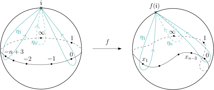
Figure 1: The marking of $\pi_{1}$ and a set of generators.

2.2 Marked projective structure and Schwarzian

The space of marked projective structures on a surface fibers over the Teichmüller space. We refer the readers to the survey paper by D. Dumas [6] for the general theory and describe here the relevant notions for the $n$-punctured sphere.

Recall that the group

$$\operatorname{PSL}(2,\mathbb{C})=\left\{A=\begin{pmatrix}a&b\\ c&d\end{pmatrix}\colon a,b,c,d\in\mathbb{C},\,ad-bc=1\right\}_{/A\sim-A}$$

acts on $\widehat{\mathbb{C}}=\mathbb{C}\mathbb{P}^{1}$ by fractional linear transformations (also called Möbius transformations) $z\mapsto(az+b)/(cz+d)$. And the subgroup

$$\mathrm{M\ddot{o}b}(\widehat{\mathbb{R}})=\operatorname{PSL}(2,\mathbb{R})=\left\{A=\begin{pmatrix}a&b\\ c&d\end{pmatrix}\colon a,b,c,d\in\mathbb{R},\,ad-bc=1\right\}_{/A\sim-A}$$

acts on $\mathbb{H}=\{z\in\widehat{\mathbb{C}}\colon\operatorname{Im}(z)>0\}$, $\widehat{\mathbb{R}}$, and $\mathbb{H}^{*}=\{z\in\widehat{\mathbb{C}}\colon\operatorname{Im}(z)<0\}$ in a similar way.

A complex projective structure $Z$ (or projective structure for short) on $\Sigma$ is a maximal atlas of projective local charts $(U,\varphi_{U})_{U\in I}$, meaning that the coordinate changes $\varphi_{V}\circ\varphi_{U}^{-1}$ belong to $\operatorname{PSL}(2,\mathbb{C})$, see Example 2.2 below.

A marked projective structure on the $n$-punctured sphere is a triple $(\Sigma,Z,f)$, where $(\Sigma,f)\in T_{0,n}$ and such that the projective structure $Z$ on $\Sigma$ induces the complex structure on $\Sigma$. We write $\mathcal{P}(\Sigma,f)$ for the set of projective structures over $(\Sigma,f)\in T_{0,n}$.

Each marked projective structure $Z$ defines a developing map and a holonomy map as follows. Here and in the sequel, let $\tilde{\Sigma}$ be the universal cover of $\Sigma$ and $\Pi:\tilde{\Sigma}\to\Sigma$ a covering map. Each projective structure on $\Sigma$ lifts to a projective structure $\tilde{Z}$ on $\tilde{\Sigma}$. A developing map of $Z$ is a holomorphic immersion $h:\tilde{\Sigma}\to\widehat{\mathbb{C}}$ such that restricting to a small open set gives a local projective chart of $\tilde{Z}$. Two developing maps $h_{1},h_{2}$ are related by $h_{1}=A\circ h_{2}$ on $\tilde{\Sigma}$ for some $A\in\operatorname{PSL}(2,\mathbb{C})$.

The group of deck transformations consists of biholomorphic functions $\alpha:\tilde{\Sigma}\to\tilde{\Sigma}$ such that $\Pi\circ\alpha=\Pi$. This group is isomorphic to $\pi_{1}(\Sigma)$ via the map sending $\alpha$ to the loop $\Pi([\alpha(x),x])$, where $x\in\tilde{\Sigma}$ is a lift of $f(\mathfrak{i})$ and $[\alpha(x),x]$ is any continuous path in $\tilde{\Sigma}$ connecting $x$ and $\alpha(x)$. Since $\pi_{1}(\Sigma)$ is further identified with the fundamental group $\pi_{1}$ of $\Sigma_{0}$ through the marking $f$, we use $\pi_{1}$ to also denote the group of deck transformations.

Since $h\circ\alpha$ is also a developing map, there is $A_{\alpha}\in\operatorname{PSL}(2,\mathbb{C})$ such that

$$A_{\alpha}\circ h=h\circ\alpha,\qquad\forall\alpha\in\pi_{1}.$$

The group homomorphism $\rho:\alpha\mapsto A_{\alpha}$, $\pi_{1}\to\operatorname{PSL}(2,\mathbb{C})$ is called the holonomy representation of $\pi_{1}$ associated with the projective structure $Z$. Post-composing $h$ by $A\in\operatorname{PSL}(2,\mathbb{C})$ conjugates the holonomy representation:

$$(h,\rho)\mapsto(A\circ h,\rho^{A}),\qquad\text{where }\rho^{A}:\alpha\mapsto A\circ A_{\alpha}\circ A^{-1}.$$ (1)

Summarizing, the projective structure $Z$ uniquely determines the development-holonomy pair $(h,\rho)$ up to the conjugation (1). Conversely, $h$ determines $Z$ as restrictions of $h\circ\pi^{-1}$ to small neighborhood in $\Sigma$ are the projective local charts.

Example 2.2.

• Trivial projective structure on $\Sigma=\widehat{\mathbb{C}}\smallsetminus\{z_{1},...,z_{n-3},0,1,\infty\}$: The developing map $h_{0}=\Pi$, and $\rho_{0}$ is the trivial representation $\pi_{1}\to\{\operatorname{Id}\}$. Hence the projective local charts are given by the identity map.

• Fuchsian projective structure $Z_{F}$ on $\Sigma$. The developing map $h_{F}$ is taken to be a uniformizing map $\tilde{\Sigma}\to\mathbb{H}$. The holonomy representation $\rho_{F}$ takes values in $\operatorname{PSL}(2,\mathbb{R})$. Moreover, $\rho_{F}(\eta_{k})$ is parabolic (recall that $\{\eta_{k}\}_{k=1,\ldots n}$ is the family of generators of $\pi_{1}$ defined above). The local charts are $h_{F}\circ\Pi^{-1}$ restricted to small enough open sets. Any other choice of the biholomorphic map $\tilde{\Sigma}\to\mathbb{H}$ is obtained from $h_{F}$ by post-composing an element of $\operatorname{PSL}(2,\mathbb{R})$, which results in the same projective structure.

The set $\mathcal{P}(\Sigma,f)$ can be parametrized using Schwarzian derivatives which compare a projective structure to the trivial projective structure: If $Z\in\mathcal{P}(\Sigma,f)$ has the development-holonomy pair $(h,\rho)$, then $h\circ h_{0}^{-1}=h\circ\Pi^{-1}$ is a multi-valued function from $\Sigma\subset\widehat{\mathbb{C}}\to\widehat{\mathbb{C}}$. In fact, for a small open set of $\Sigma$, two choices of lift $\Pi^{-1}$ are related by $\hat{\Pi}^{-1}=\alpha\circ\Pi^{-1}$ for some $\alpha\in\pi_{1}:\tilde{\Sigma}\to\tilde{\Sigma}$. And

$$h\circ\hat{\Pi}^{-1}=h\circ\alpha\circ\Pi^{-1}=\rho(\alpha)\circ h\circ\Pi^{-1}.$$ (2)

Recall that the Schwarzian derivative of a holomorphic immersion, defined as

$$\mathcal{S}[\varphi]=\frac{\varphi^{\prime\prime\prime}}{\varphi^{\prime}}-\frac{3}{2}\left(\frac{\varphi^{\prime\prime}}{\varphi^{\prime}}\right)^{2},$$

satisfies $\mathcal{S}[A]\equiv 0$ for all $A\in\operatorname{PSL}(2,\mathbb{C})$ and the chain rule

$$\mathcal{S}[\varphi\circ\psi]=\mathcal{S}[\varphi]\circ\psi(\psi^{\prime})^{2}+\mathcal{S}[\psi].$$ (3)

Informally, the Schwarzian derivative measures the local deviation of a holomorphic immersion from an Möbius transformation. In particular, (2) shows that although $h\circ h_{0}^{-1}$ is multi-valued, its Schwarzian is a well-defined holomorphic function on $\Sigma$:

$$\mathcal{S}[h\circ\hat{\Pi}^{-1}]=\mathcal{S}[h\circ\Pi^{-1}].$$

Any other developing map of $Z$ is obtained from the transformation (1), which gives the same Schwarzian derivative $S[h\circ\Pi^{-1}]$.

Lemma 2.3.

Each projective structure $Z\in\mathcal{P}(\Sigma,f)$ uniquely defines a quadratic differential $q=\mathcal{S}[h\circ\Pi^{-1}]\,\mathrm{d}z^{2}$ on $\Sigma$, where $h$ is any developing map of $Z$. If $Z_{1}$ and $Z_{2}\in\mathcal{P}(\Sigma,f)$ define the same quadratic differential, then $Z_{1}=Z_{2}.$

Proof.

The function $q$ is a quadratic differential since if $A\in\operatorname{PSL}(2,\mathbb{C})$ and $\Sigma=A(\Sigma_{1})$, then the corresponding quadratic differential $q_{1}$ on $\Sigma_{1}$ transforms like

$$q_{1}=\mathcal{S}[h\circ\Pi^{-1}\circ A]\,\mathrm{d}z^{2}=q(A)(A^{\prime})^{2}\mathrm{d}z^{2}=A^{*}q$$ (4)

by the chain rule (3).

For the second claim, let $h_{j}$ be a developing map of $Z_{j}$, then the assumption $\mathcal{S}[h_{1}\circ\Pi^{-1}]=\mathcal{S}[h_{2}\circ\Pi^{-1}]$ shows that there exists $A\in\operatorname{PSL}(2,\mathbb{C})$ such that $h_{2}=A\circ h_{1}$. Therefore, the restrictions of $h_{1}$ and $h_{2}$ to small open sets are compatible projective charts and $Z_{1}=Z_{2}$. ∎

2.3 Loewner energy of curves and loops

In this section, we recall the definition and basic facts about Loewner energy.

We say that $\gamma$ is a simple curve in $(D;a,b)$, if $D$ is a simply connected domain, $a,b$ are two distinct prime ends of $D$, and $\gamma$ has a continuous and injective parametrization $(0,T)\to D$ such that $\gamma(t)\to a$ as $t\to 0$ and $\gamma(t)\to c\in D\cup\{b\}$ as $t\to T$. If $c=b$ then we say $\gamma$ is a chord in $(D;a,b)$.

Simple chords in $(\mathbb{H};0,\infty)$ can be encoded into a chordal driving function as follows (this procedure is called the Loewner transform). We first parameterize the curve by the half-plane capacity. More precisely, $\gamma$ is continuously parametrized by $[0,T]$, where $T\in(0,\infty]$ with $\gamma(0)=0$, such that the unique conformal map $g_{t}$ from ${\mathbb{H}}\smallsetminus\gamma[0,t]$ onto ${\mathbb{H}}$ with the expansion at infinity $g_{t}(z)=z+o(1)$ satisfies

$$g_{t}(z)=z+\frac{2t}{z}+o\left(\frac{1}{z}\right),\qquad\forall t\in(0,T).$$ (5)

The coefficient $2t$ is the half-plane capacity of $\gamma[0,t]$, and $2T$ is the total capacity of $\gamma$. The map $g_{t}$ can be extended by continuity to the boundary point $\gamma(t)$ and that the real-valued function $W(t):=g_{t}(\gamma(t))$ is continuous with $W(0)=0$ (i.e., $W\in C^{0}[0,T]$). This function $W$ is called the driving function of $\gamma$. The Loewner transform satisfies the following properties:

• (Additivity) Fix $s>0$, the driving function generating $(\overline{g_{s}(\gamma[s,t])}-W(s))_{t\in[0,T-s]}$ is $t\mapsto W(s+t)-W(s)$.

• (Scaling) Fix $\lambda>0$, the driving function generating the scaled and capacity-reparameterized curve $(\lambda\gamma(\lambda^{-2}t))_{t\in[0,\lambda^{2}T]}$ is $t\mapsto\lambda W(\lambda^{-2}t)$.

Definition 2.4.

Let $\gamma$ be a simple curve in $(D;a,b)$. Let $\phi$ be a conformal map from $D$ onto $\mathbb{H}$ with $\phi(a)=0$, $\phi(b)=\infty$, $T$ be the half-plane capacity of $\phi(\gamma)$. The chordal Loewner energy of $\gamma$ in $(D;a,b)$ is

$$I_{D;a,b}(\gamma):=I_{\mathbb{H};0,\infty}(\phi(\gamma)):=\frac{1}{2}\int_{0}^{T}\dot{W}(t)^{2}dt\in[0,\infty]$$

if the chordal driving function $W$ of $\phi(\gamma)$ is absolutely continuous, and $\infty$ otherwise.

If $\gamma$ makes it all the way to $b$ (namely, if $\gamma$ is a chord) and if $I_{D;a,b}(\gamma)<\infty$ then $T=\infty$ (namely, $\gamma$ has infinite total capacity).

Note that the definition does not depend on the conformal map $\phi$ chosen since, from the scaling property of the driving function, we have that for all $\lambda>0$, $I_{\mathbb{H},0,\infty}(\gamma)=I_{\mathbb{H},0,\infty}(\lambda\gamma)$.

Remark 2.5.

The Loewner energy of a chord attains its minimum $0$ if and only if the driving function is constantly $0$, namely $\phi(\gamma)$ is $\mathfrak{i}\mathbb{R}_{+}$ which is equivalent to the curve $\gamma$ being the hyperbolic geodesic of $D$ from $a$ to $b$. We note that a hyperbolic geodesic is an analytic curve.

The additivity of the Loewner transform immediately implies the following lemma.

Lemma 2.6 (Additivity of Loewner energy).

For any continuous parametrization $\gamma:[0,1]\to D$ with $\gamma(0)=a$ and $\gamma(1)=b$, and for any $t<1$, we have

$$I_{D;a,b}(\gamma[0,1])=I_{D;a,b}(\gamma[0,t])+I_{D\smallsetminus\gamma[0,t];\gamma(t),b}(\gamma[t,1]).$$

We note that although $\gamma$ is not necessarily parametrized by capacity, $I_{D;a,b}(\gamma[0,1])$ is understood as in Definition 2.4 where we start with parametrizing $\phi(\gamma)$ by capacity. Thus $I_{D;a,b}(\gamma[0,1])$ is trivially invariant under increasing parametrization. It was also shown in [23] that the chordal Loewner energy does not depend on the orientation of the curve. Therefore, we may view the curves as being unoriented.

Let us next recall the definition of Loewner energy for Jordan curves, introduced in [17]. Let $\gamma:[0,1]\to\widehat{\mathbb{C}}:=\mathbb{C}\cup\{\infty\}$ be a continuously parametrized Jordan curve with the marked point $\gamma(0)=\gamma(1)$. For every $\varepsilon>0$, $\gamma[\varepsilon,1]$ is a chord connecting $\gamma(\varepsilon)$ to $\gamma(1)$ in the simply connected domain $\widehat{\mathbb{C}}\smallsetminus\gamma[0,\varepsilon]$.

Definition 2.7.

The Loewner energy of $\gamma$ rooted at $\gamma(0)$ is

$$I^{L}(\gamma,\gamma(0)):=\lim_{\varepsilon\to 0}I_{\widehat{\mathbb{C}}\smallsetminus\gamma[0,\varepsilon];\gamma(\varepsilon),\gamma(0)}(\gamma[\varepsilon,1]).$$

The third and fourth authors proved the following result.

Theorem 2.8 (​​ [17]).

The Loewner energy of the rooted Jordan curve does not depend on the root chosen.

Hence, the Loewner energy is a quantity on the family of unrooted Jordan curves that is invariant under Möbius transformations. The root independence is further explained by the following equivalent expression of the Loewner energy involving only two conformal maps.

Theorem 2.9 ([24, Thm. 1.3]).

Let $\gamma$ be a bounded Jordan curve. Let $\Omega_{+}$ and $\Omega_{-}$ denote respectively the bounded and unbounded components of $\mathbb{C}\smallsetminus\gamma$. Let $g_{+}$ be a conformal map from $\Omega_{+}$ onto $\mathbb{D}$ and $g_{-}$ a conformal map from $\Omega_{-}$ onto $\mathbb{D}^{*}$ fixing $\infty$, we have the identity

$$I^{L}(\gamma)=\mathcal{D}_{\Omega_{+}}(\log\left\lvert g_{+}^{\prime}\right\rvert)+\mathcal{D}_{\Omega_{-}}(\log\left\lvert g_{-}^{\prime}\right\rvert)-4\log\left\lvert g_{+}^{\prime}(0)\right\rvert+4\log\left\lvert g_{-}^{\prime}(\infty)\right\rvert,$$ (6)

where $g_{-}^{\prime}(\infty):=\lim_{z\to\infty}g_{-}^{\prime}(z)$ and $\mathcal{D}_{\Omega}(u)=\int_{\Omega}\left\lvert\nabla u\right\rvert^{2}/\pi\,|\mathrm{d}z|^{2}$ denotes the Dirichlet energy of $u$ on $\Omega$.

This result also identifies the family of Jordan curves with finite energy with the family of Weil–Petersson quasicircles introduced in [21] where the right-hand side of (6) is called universal Liouville action. This family of Jordan curves has been the topic of very active research thanks to a large number of very different but equivalent descriptions [1, 19, 25, 4, 9, 10, 3].

2.4 Energy minimizers and the geodesic property

In this section, we study the basic properties of energy-minimizing chords and loops.

Lemma 2.10 ([23, Prop. 3.1]).

Let $\theta\in(0,\pi)$. The Loewner energy of any chord in $(\mathbb{H};0,\infty)$ passing through $z=e^{\mathfrak{i}\theta}$ is larger or equal to $-8\log\sin(\theta)$. The minimum is attained by a unique chord $\gamma^{z}$.

The energy minimizer turns out to be the unique $C^{1}$ smooth chord with the following geodesic property. It will be an essential building block in studying the Jordan curves with geodesic property.

Definition 2.11.

Let $z\in D$ be an interior point of $D$. We define a geodesic pair in $(D;a,b;z)$ to be a chord $\gamma$ in $(D;a,b)$ such that $\gamma=\gamma_{1}\cup\gamma_{2}$, $\gamma_{1}\cap\gamma_{2}=\{z\}$, $\gamma_{1}$ is the geodesic in $(D\smallsetminus\gamma_{2};a,z)$ and $\gamma_{2}$ is the geodesic in $(D\smallsetminus\gamma_{1};z,b)$.

Lemma 2.12.

The energy minimizing chord $\gamma^{z}$ is a geodesic pair in $(\mathbb{H};0,\infty;z)$ and is $C^{1,1-\varepsilon}$ for all $\varepsilon>0$.

Proof.

We write $\gamma^{z}=\gamma_{1}\cup\gamma_{2}$ such that $\gamma_{1}$ has the end points $a$ and $z$ and $\gamma_{2}$ has the end points $z$ and $b$. Lemma 2.6 shows that

$$I_{D;a,b}(\gamma^{z})=I_{D;a,b}(\gamma_{1})+I_{D\smallsetminus\gamma_{1};z,b}(\gamma_{2}).$$

Since $\gamma^{z}$ is minimizing the energy among all chords passing through $z$, $I_{D\smallsetminus\gamma_{1};z,b}(\gamma_{2})=0$. Otherwise, replacing $\gamma_{2}$ by the geodesic in $(D\smallsetminus\gamma_{1};z,b)$ decreases the energy. Similarly, considering $\gamma$ as a chord in $(D;b,a)$ shows that $\gamma_{1}$ is the hyperbolic geodesic in $(D\smallsetminus\gamma_{2};z,a)$.

The regularity of $\gamma^{z}$ follows from the fact that the driving function of $\gamma^{z}$ is $C^{1,1/2}$ regular. In fact, the driving function of $\gamma^{z}$ is studied in [23], see e.g. Equation (3.2) there. The main theorem of [27] shows that $\gamma^{z}$ is weakly $C^{1,1}$ (which implies that $\gamma^{z}$ is $C^{1,1-\varepsilon}$) regular. ∎

Remark 2.13.

The regularity of a $C^{1}$ geodesic pair at its vertex can also be seen from Lemma 2.19 below.

In the companion paper [12], we classified all geodesic pairs in $(\mathbb{H};0,\infty;z)$. In particular, [12, Thm. 3.9] shows that there is a unique $C^{1}$ smooth geodesic pair in $(\mathbb{H};0,\infty;z)$, hence the energy minimizer; [12, Cor. 3.10] shows that if a geodesic pair is not $C^{1}$, then it has a logarithmic spiral near $z$ which has necessarily infinite energy.

Corollary 2.14.

The energy minimizer $\gamma^{z}$ is the unique $C^{1}$ smooth geodesic pair in $(\mathbb{H};0,\infty;z)$.

Let us now move to the loop case. A Jordan curve $\gamma\subset\widehat{\mathbb{C}}$ through distinct points $z_{1},...,z_{n}$ is called piecewise geodesic if $\gamma\smallsetminus\{z_{1},...,z_{n}\}=\gamma_{1}\cup\gamma_{2}\cup\ldots\cup\gamma_{n}$ where $\gamma_{j}$ is a hyperbolic geodesic in $\widehat{\mathbb{C}}\smallsetminus(\gamma\smallsetminus\gamma_{j})$ for all $j=1,\ldots,n$. We also say that $\gamma$ has the geodesic property. Such curves arise naturally as Loewner energy minimizers:

Lemma 2.15.

There exists at least one minimizer of the Loewner energy in each isotopy class $\mathcal{L}(z_{1},z_{2},\cdots,z_{n};\tau)$. Any minimizer has the geodesic property and is $C^{1,1-\varepsilon}$ regular for all $\varepsilon>0$.

Proof.

In [17, Prop. 2.13], it was shown that there exists at least one minimizer of the Loewner energy passing through a collection of distinct points $z_{1},z_{2},\cdots,z_{n}$ (without the constraint on the isotopy class). The same proof can be easily modified to show that each isotopy class $\mathcal{L}(z_{1},z_{2},\cdots,z_{n};\tau)$ contains at least one energy minimizer by taking an energy-minimizing sequence within the isotopy class and passing it to a subsequential limit. For the geodesic property, it follows from the root-invariance (Theorem 2.8, Theorem 2.9) and the additivity Lemma 2.6 that $\gamma_{k-1}\cup\gamma_{k}$ has to be an energy minimizing chord through $z_{k}$ in $(\Omega_{+}\cup\Omega_{-}\cup\gamma_{k-1}\cup\gamma_{k};z_{k-1},z_{k+1})$ for every $k$. Lemma 2.12 then shows that it is a geodesic pair with $C^{1,1-\varepsilon}$ regularity which implies the geodesic property of $\gamma$ with the same regularity. ∎

Remark 2.16.

One may wonder if the geodesic property is related to the hyperbolic geodesics in the $n$-punctured sphere. [12, Lem. 4.2] shows that they are very different. In fact, if $\gamma$ is a Jordan curve with the geodesic property and if each arc $\gamma_{k}$ is a hyperbolic geodesic in the punctured sphere $\Sigma:=\widehat{\mathbb{C}}\smallsetminus\{z_{1},\ldots,z_{n}\}$ between $z_{k}$ and $z_{k+1}$, then $\gamma$ is a circle. In Section 6, we show that they are related by a $\pi$-angle grafting.

The geodesic property can easily be characterized in terms of conformal welding.

More precisely, let $\gamma$ be a Jordan curve through points $z_{1},\ldots,z_{n}$ (in this order), let $\Omega_{+}$ be the connected component of $\widehat{\mathbb{C}}\smallsetminus\gamma$ where $(z_{1},\ldots,z_{n})$ goes around $\Omega_{+}$ counterclockwisely, and denote $\Omega_{-}$ the other connected component. Let $g_{+}$ and $g_{-}$ be respectively a conformal map from $\Omega_{+}$ onto $\mathbb{H}$ and from $\Omega_{-}$ onto $\mathbb{H}^{*}$. Then the welding homeomorphism of $\gamma$ is given by $\varphi:=g_{-}\circ g_{+}^{-1}|_{\widehat{\mathbb{R}}}.$ It is determined by $\gamma$ only up to pre- and post-composition with Möbius automorphisms in $\operatorname{PSL}(2,\mathbb{R})$. Let $x_{k}=g_{+}(z_{k})$ and $y_{k}=g_{-}(z_{k})=\varphi(x_{k}).$ A homeomorphism $\varphi$ of $\widehat{\mathbb{R}}$ is called piecewise Möbius if $\widehat{\mathbb{R}}$ can be decomposed into finitely many intervals such that on each interval, $\varphi$ is (the restriction of) a Möbius automorphisms.

Theorem 2.17 ([12, Cor. 4.1 and Lem. 4.12]).

A Jordan curve $\gamma$ has the geodesic property if and only if the welding homeomorphism $w$ is piecewise Möbius. Moreover, $\gamma$ is $C^{1}$ smooth if and only if the welding $\varphi$ is $C^{1}$ smooth.

2.5 Geodesic pairs and conformal welding

In this section, we study the conformal welding of geodesic pairs. These auxiliary results will be used in Sections 4 and 5 to pinpoint the local behavior of the welding maps of piecewise geodesic loops.

Let us consider $\theta\in(0,\pi)$ and the geodesic pair $\gamma$ in $(\mathbb{D};e^{-\mathfrak{i}\theta},e^{\mathfrak{i}\theta};0)$. We write $\gamma=\gamma_{1}\cup\gamma_{2}$ where $\gamma_{1}$ connects $e^{\mathfrak{i}\theta}$ to $0$ and $\gamma_{2}$ connects $e^{-\mathfrak{i}\theta}$ to $0$. As shown in [12], the map

$$h_{\theta}(z)=G_{\pi/2-\theta}(\mathfrak{i}z)=\frac{1}{2}\left(\mathfrak{i}z+\frac{1}{\mathfrak{i}z}\right)-\mathfrak{i}\cos(\theta)\log(\mathfrak{i}z)$$

maps the two connected components of $\mathbb{D}\smallsetminus\gamma$ to upper and lower half-planes. Here the branch of $\log(\mathfrak{i}z)$ is chosen so that the imaginary part is $\pi/2$ for $z\in(0,1)$ and the branch cut is along $\gamma_{1}$. See Figure 2 for an illustration.

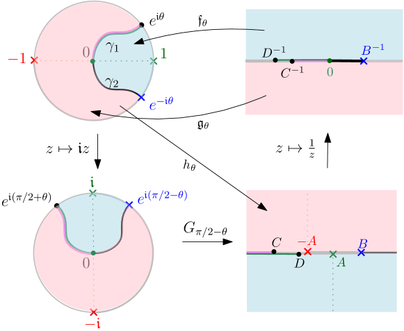
Figure 2: Illustration of the uniformizing conformal maps associated with a standard geodesic pair in $(\mathbb{D};e^{\mathfrak{i}\theta},e^{-\mathfrak{i}\theta};0)$. It was computed in [12] (see Figure 1 there) that $A=(\pi/2)\cos(\theta)$, $B=\sin(\theta)+(\pi/2-\theta)\cos(\theta)$, $C=-2A-B$, $D=2A-B$.

The map $h_{\theta}$ is analytic in $\mathbb{D}\smallsetminus\gamma_{1}$ and satisfies $h_{\theta}(0)=\infty$, $h_{\theta}(1)=-h_{\theta}(-1)=A:=(\pi/2)\cos(\theta)$ and $h(e^{-\mathfrak{i}\theta})=B:=\sin(\theta)+(\pi/2-\theta)\cos(\theta)$. The point $e^{\mathfrak{i}\theta}$ gets mapped to either $C=-2A-B$ or $D=2A-B$, depending on the side of the approach.

Finally, we define the conformal maps $\mathfrak{f}_{\theta}(z)=h_{\theta}^{-1}(1/z)$ (for $z\in\mathbb{H}$) and $\mathfrak{g}_{\theta}(z)=h_{\theta}^{-1}(1/z)$ (for $z\in\mathbb{H}^{*}$). They both map $0$ to $0$ and extend continuously to the boundary.

Lemma 2.18.

Let $\varphi_{\theta}\colon[1/D,1/B]\to[1/C,1/B]$ be the welding homeomorphism $\varphi_{\theta}(x)=(\mathfrak{g}_{\theta}^{-1}\circ\mathfrak{f}_{\theta})(x)$ for the geodesic pair. Then

$$\varphi_{\theta}(x)=\begin{cases}\dfrac{x}{(C-D)x+1},&\text{if }x\in[1/D,0]\\ x,&\text{if }x\in[0,1/B]\end{cases}$$

Moreover, the jump

$$\lambda[\varphi_{\theta}](0):=\varphi_{\theta}^{\prime\prime}/\varphi_{\theta}^{\prime}(0{\scriptstyle+})-\varphi_{\theta}^{\prime\prime}/\varphi_{\theta}^{\prime}(0{\scriptstyle-})$$ (7)

of the pre-Schwarzian $\varphi_{\theta}^{\prime\prime}/\varphi_{\theta}^{\prime}$ at $0$ equals $-4\pi\cos(\theta)$.

Proof.

It was computed in [12] that the welding homeomorphism $\omega$ for $h_{\theta}^{-1}$ (i.e. without composing with $1/z$, which also swaps upper and lower half-planes) is given by $\omega(x)=x+D-C$ when $x<C$ and $\omega(x)=x$ when $x>B$. The first claim follows since we have $\varphi_{\theta}(x)=1/\omega^{-1}(1/x)$. We note that the pre-Schwarzian of $\varphi_{\theta}$ is

$$\dfrac{\varphi_{\theta}^{\prime\prime}(x)}{\varphi_{\theta}^{\prime}(x)}=\begin{cases}\dfrac{-2(C-D)}{(C-D)x+1},&\text{when }x\in[1/D,0)\\ 0,&\text{when }x\in(0,1/B]\end{cases}$$

In particular,

$$\lambda[\varphi_{\theta}](0)=2(C-D)=-8A=-4\pi\cos(\theta).\qed$$

We will also need precise asymptotics of $\mathfrak{f}_{\theta}$ and $\mathfrak{g}_{\theta}$ at $0$.

Lemma 2.19.

We have the following asymptotic expansions as $z\to 0$:

$$\mathfrak{f}_{\theta}(z) =\frac{1}{2\mathfrak{i}}z-\frac{1}{2}\cos(\theta)z^{2}\log(z)+O(z^{2})$$

$$\mathfrak{f}_{\theta}^{\prime}(z) =\frac{1}{2\mathfrak{i}}-\cos(\theta)z\log(z)+O(z)$$

$$\partial_{\theta}\mathfrak{f}_{\theta}(z) =\frac{1}{2}\sin(\theta)z^{2}\log(z)+O(z^{2})$$

The same asymptotics hold with $\mathfrak{f}_{\theta}$ replaced by $\mathfrak{g}_{\theta}$.

Proof.

Let us write $\mathfrak{f}_{\theta}(z)=w$. By definition, we have

$$z=\mathfrak{f}_{\theta}^{-1}(w)=\frac{1}{h_{\theta}(w)}=\frac{2\mathfrak{i}w}{1+2\cos(\theta)w\log(\mathfrak{i}w)-w^{2}}.$$

Note that since $w\to 0$ as $z\to 0$, this implies that $|z|\geq|w|$ for $z$ small enough, so that

$$w=O(z).$$

We next write the above equation as

$$z=2\mathfrak{i}w-\frac{4\mathfrak{i}\cos(\theta)w^{2}\log(\mathfrak{i}w)-2\mathfrak{i}w^{3}}{1+2\cos(\theta)w\log(\mathfrak{i}w)-w^{2}},$$

implying that

$$w=\frac{z}{2\mathfrak{i}}+\frac{2\cos(\theta)w^{2}\log(\mathfrak{i}w)-w^{3}}{1+2\cos(\theta)w\log(\mathfrak{i}w)-w^{2}}=\frac{z}{2\mathfrak{i}}+2\cos(\theta)w^{2}\log(\mathfrak{i}w)+O(w^{2}).$$

In particular, $w=O(z)$ now implies that $w=z/(2\mathfrak{i})+O(z^{2}\log(z))=z/(2\mathfrak{i})+o(z)$, so that $w^{2}=-z^{2}/4+O(z^{3}\log(z))$ and $\log(\mathfrak{i}w)=\log(z/2+o(z))=\log(|z/2||1+o(1)|)+O(1)=\log(|z|)+O(1)=\log(z)+O(1).$ This gives us the first asymptotics in the statement,

$$\mathfrak{f}_{\theta}(z)=w=\frac{z}{2\mathfrak{i}}-\frac{1}{2}\cos(\theta)z^{2}\log(z)+O(z^{2}).$$

Next, we note that

$$(\mathfrak{f}_{\theta}^{-1})^{\prime}(w)=\frac{2\mathfrak{i}-4\mathfrak{i}\cos(\theta)w+2\mathfrak{i}w^{2}}{(1+2\cos(\theta)w\log(\mathfrak{i}w)-w^{2})^{2}},$$

so that

$$\mathfrak{f}_{\theta}^{\prime}(z)=\frac{1}{(\mathfrak{f}_{\theta}^{-1})^{\prime}(w)}=\frac{1+4\cos(\theta)w\log(\mathfrak{i}w)+O(w)}{2\mathfrak{i}+O(w)}.$$

Applying the asymptotics for $w$ obtained above, we get

$$\mathfrak{f}_{\theta}^{\prime}(z)=\frac{1}{2\mathfrak{i}}-\cos(\theta)z\log(z)+O(z)$$

as wanted. Finally, note that differentiating the identity $\mathfrak{f}_{\theta}(\mathfrak{f}_{\theta}^{-1}(w))=w$ with respect to $\theta$ on both sides gives us

$$\partial_{\theta}\mathfrak{f}_{\theta}(\mathfrak{f}_{\theta}^{-1}(w))+\mathfrak{f}_{\theta}^{\prime}(\mathfrak{f}_{\theta}^{-1}(w))\partial_{\theta}[\mathfrak{f}_{\theta}^{-1}](w)=0,$$

so that

$$\partial_{\theta}\mathfrak{f}_{\theta}(z)=-\mathfrak{f}_{\theta}^{\prime}(z)\partial_{\theta}[\mathfrak{f}_{\theta}^{-1}](w)=-\mathfrak{f}_{\theta}^{\prime}(z)\left(\frac{4\mathfrak{i}\sin(\theta)w^{2}\log(\mathfrak{i}w)}{(1+2\cos(\theta)w\log(\mathfrak{i}w)-w^{2})^{2}}\right).$$

Again, applying the already obtained asymptotics for $w$ gives us

$$\partial_{\theta}\mathfrak{f}_{\theta}(z)=\frac{1}{2}\sin(\theta)z^{2}\log(z)+O(z^{2}).$$

The same proof goes through verbatim for $\mathfrak{g}_{\theta}$ as well. ∎

We conclude this section with a warning to the reader: We will sometimes use the notation $g_{+},g_{-}$ and sometimes the notation $f,g$ for conformal maps associated with the two sides of a Jordan curve.

3 Uniqueness of piecewise geodesic $C^{1}$ Jordan curves

In this section, we will prove that every isotopy class $\mathcal{L}(z_{1},\dots,z_{n};\tau)$ contains a unique piecewise geodesic $C^{1}$ smooth Jordan curve. It follows in particular that the minimizer of Loewner energy obtained in Lemma 2.15 is unique.

Theorem 3.1.

Let $\gamma,\tilde{\gamma}\in\mathcal{L}(z_{1},\dots,z_{n};\tau)$ be two isotopic $C^{1}$ smooth Jordan curves. If $\gamma$ and $\tilde{\gamma}$ are piecewise geodesic, then $\gamma=\tilde{\gamma}$.

Roughly speaking, our proof will be based on constructing for each boundary arc $\gamma_{k}$ a suitable ‘distance’ or ‘potential’ function $h_{k}$ on the sphere and then using it to measure how far the corresponding arc $\tilde{\gamma}_{k}$ of $\tilde{\gamma}$ lies from $\gamma_{k}$, with the goal being to show that $h_{k}|_{\tilde{\gamma}_{k}}=0$. As the hyperbolic geodesic $\gamma_{k}$ consists of exactly those points which get mapped to the real axis when the domain $(\widehat{\mathbb{C}}\smallsetminus\gamma)\cup\gamma_{k}$ is mapped conformally to the strip $\{z\in\mathbb{C}:\operatorname{Im}(z)\in(-1,1)\}$, a natural candidate for $h_{k}$ is the imaginary part of this mapping. When trying to implement such a strategy, one quickly notices that $\tilde{\gamma}_{k}$ may get further away from $\gamma_{k}$ by going through other arcs of $\gamma$. It is therefore natural to shift our viewpoint from the sphere to the universal cover of $\Sigma$. For this purpose, let us fix some notation.

We let $\Pi\colon\mathbb{D}\to\Sigma$ be a holomorphic universal covering. The set $\Pi^{-1}(\gamma)$ is the union of countably many arcs $\ell_{\alpha}\subset\mathbb{D}$, each of them a lift of a single $\gamma_{k}$ for some $k\in\{1,\dots,n\}$. Here $\alpha\in I$ runs over some abstract index set $I$.

Each $\ell_{\alpha}$ in turn will be a hyperbolic geodesic in a domain $U_{\alpha}\subset\mathbb{D}$, corresponding to a lift of $\Omega_{+}\cup\Omega_{-}\cup\Pi(\ell_{\alpha})$. Moreover, each $U_{\alpha}$ naturally splits into subdomains $U_{\alpha}^{+}$ and $U_{\alpha}^{-}$ so that $\Pi(U_{\alpha}^{\pm})=\Omega_{\pm}$. Note that $U_{\alpha}$ is a fundamental domain of the covering $\Pi$, so that its translates by the deck transformations form a tiling of $\mathbb{D}$. It follows that also the domains $U_{\beta}^{\pm}$ ($\beta\in I$) form a tiling of $\mathbb{D}$ (with each tile appearing $n$ times).

Let next $f\colon[0,1]\times\Sigma\to\Sigma$ be an isotopy of $\Sigma$ such that $f_{0}(\gamma)=\gamma$ and $f_{1}(\gamma)=\tilde{\gamma}$. Then $f$ admits a lift $\hat{f}\colon[0,1]\times\mathbb{D}\to\mathbb{D}$ to the universal cover of $\Sigma$ such that $\hat{f}_{t}|_{\partial D}=\operatorname{Id}$ for all $t\in[0,1]$, see [11, V.1.4]. We use $\hat{f}$ to define the arcs and domains $\tilde{\ell}_{\alpha}=\hat{f}(\ell_{\alpha})$, $\tilde{U}_{\alpha}=\hat{f}(U_{\alpha})$ and $\tilde{U}_{\alpha}^{\pm}=\hat{f}(U_{\alpha}^{\pm})$ corresponding to the curve $\tilde{\gamma}$. Note in particular that $\ell_{\alpha}$ and $\tilde{\ell}_{\alpha}$ share the same endpoints.

We will next define, for each fixed $\alpha\in I$, a potential function $h_{\alpha}$ as hinted above. We start by constructing a tree $\mathcal{T}$ on $I$ where we connect two distinct labels $\nu,\mu\in I$ by an edge if either $U_{\nu}^{+}=U_{\mu}^{+}$ or $U_{\nu}^{-}=U_{\mu}^{-}$. In other words, there is an edge between $\nu$ and $\mu$ if $\ell_{\nu}$ and $\ell_{\mu}$ are both part of the boundary of a common tile. The graph obtained is a tree since every arc $\ell_{\nu}$ cuts $\mathbb{D}$ in two disjoint pieces. We let $d$ denote the graph distance in this tree and also let

$$\sigma(\alpha,\nu)=\begin{cases}0,&\text{if }\alpha=\nu\\ 1,&\text{if the path from }\alpha\text{ to }\nu\text{ goes through some }\mu\neq\alpha\text{ with }\ell_{\mu}\subset\partial U_{\alpha}^{+}\\ -1,&\text{if the path from }\alpha\text{ to }\nu\text{ goes through some }\mu\neq\alpha\text{ with }\ell_{\mu}\subset\partial U_{\alpha}^{-}\end{cases}$$

Finally, we let $h_{\alpha}\colon\mathbb{D}\to\mathbb{R}$ be the function which is harmonic outside of $\Pi^{-1}(\gamma)$ and which on any given arc $\ell_{\nu}$ ($\nu\in I$) takes the constant value $\sigma(\alpha,\nu)d(\alpha,\nu)$. For later purposes, let us also denote by $\mathcal{T}_{\alpha}$ the tree $\mathcal{T}$ with a distinguished root at $\alpha$, which also defines a partial order $\leq_{\alpha}$ by letting $\mu\leq_{\alpha}\nu$ if $\nu$ is a descendant of $\mu$ in $\mathcal{T}$.

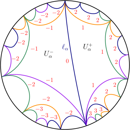
Figure 3: The covering space picture. The values of $h_{\alpha}$ on the arcs $\ell_{\beta}$ are written in red. Arcs with the same color are equivalent under the deck transformations.

As stated in the beginning, we aim to show that $h_{\alpha}$ vanishes on $\tilde{\ell}_{\alpha}$. We begin by showing that it is bounded.

Lemma 3.2.

There exists a constant $C>0$ such that $|h_{\alpha}(z)|\leq C$ for all $\alpha\in I$ and $z\in\tilde{\ell}_{\alpha}$.

Proof.

Note that since $\gamma$ and $\tilde{\gamma}$ are $C^{1}$ smooth arcs, $\tilde{\gamma}_{k}$ cannot hit both $\gamma_{k}$ and $\gamma_{k+1}$ (resp. $\gamma_{k-1}$) infinitely many times as it approaches $z_{k+1}$ (resp. $z_{k}$). It follows that if $\tilde{\ell}_{\alpha}$ is a lift of $\tilde{\gamma}_{k}$, it intersects at most finitely many domains $U_{\beta}$ and hence $|h_{\alpha}|$ is bounded on $\tilde{\ell}_{\alpha}$. The bound obtained does not depend on the particular lift. ∎

Let us next define the auxiliary function $\hat{\rho}\colon\mathbb{D}\to\mathbb{R}$ by setting $\hat{\rho}(z)=|h_{\alpha}(z)|$ for all $z\in\tilde{\ell}_{\alpha}$ and extending harmonically inside each tile $\tilde{U}_{\alpha}$. Note that $\hat{\rho}$ is invariant under the deck transformations of the covering $\Pi$, and hence there exists a continuous and bounded function $\rho\colon\Sigma\to\mathbb{R}$ such that $\hat{\rho}=\rho\circ\Pi$. The following could be considered the main lemma of our proof as it implies that $\rho$ has to be a constant.

Lemma 3.3.

The function $\rho$ is subharmonic.

Before proving the lemma, let us state and prove a couple of auxiliary results. We begin with the following elementary criterion for subharmonicity.

Lemma 3.4.

Suppose that $f\colon\mathbb{D}\to\mathbb{R}$ satisfies the following property: For every $z\in\mathbb{D}$, there exists a subharmonic function $u$ defined in a neighborhood of $z$ such that $u\leq f$ and $u(z)=f(z)$. Then $f$ is subharmonic.

Proof.

It is straightforward to check that the sub-mean value property of $f$ at $z$ follows from that of $u$. ∎

A second auxiliary result we will use is the subharmonicity of $|h_{\alpha}|$ itself.

Lemma 3.5.

The function $h_{\alpha}$ is harmonic in $U_{\alpha}$ and $|h_{\alpha}|$ is subharmonic in $\mathbb{D}$.

Proof of Lemma 3.5.

The harmonicity of $h_{\alpha}$ in $U_{\alpha}$ follows from the assumption that $\ell_{\alpha}$ is a hyperbolic geodesic in $U_{\alpha}$: Indeed, $h_{\alpha}$ coincides with the imaginary part of a conformal map from $U_{\alpha}$ to the strip $\{z\in\mathbb{C}:\operatorname{Im}(z)\in(-1,1)\}$ mapping the two boundary components $\partial U_{\alpha}^{\pm}\smallsetminus\ell_{\alpha}$ to the horizontal lines $\operatorname{Im}(w)=\pm 1$, respectively. Clearly, in the strip, the hyperbolic geodesic between $-\infty$ and $+\infty$ is the real line $\operatorname{Im}(w)=0$.

To show that $|h_{\alpha}|$ is subharmonic, we will verify the condition of Lemma 3.4. As $h_{\alpha}$ is harmonic and has a constant sign in each tile $U_{\beta}^{\pm}$, it is enough to consider the case $z\in\ell_{\beta}$ for some $\beta\in I$. Moreover, by symmetry, we may assume that $\sigma(\alpha,\beta)=1$. Consider the harmonic function $u$ in the domain $U_{\beta}$ which takes value $d(\alpha,\beta)+1$ on every boundary arc $\ell_{\nu}\subset\partial U_{\beta}$ such that $\nu>_{\alpha}\beta$ and $d(\alpha,\beta)-1$ on every other boundary arc. Clearly $u$ equals $|h_{\alpha}|$ on $\ell_{\beta}$ as well as on the boundary arcs $\ell_{\nu}$ for which $\nu>_{\alpha}\beta$. If $\mu$ is the parent in $\mathcal{T}_{\alpha}$ of $\beta$ we also have $u(w)=|h_{\alpha}(z)|$ for $w\in\ell_{\mu}$, while for $w$ on the rest of the boundary arcs we have $u(z)=|h_{\alpha}(z)|-1$. Thus $u\leq|h_{\alpha}|$ on the boundary of $U_{\beta}$ and hence also in $U_{\beta}$. ∎

The third and final result we need before proving Lemma 3.3 is the following inequality.

Lemma 3.6.

We have $|h_{\beta}|\geq|h_{\alpha}\mp 1|$ whenever $\ell_{\beta}\subset\partial U_{\alpha}^{\pm}\smallsetminus\ell_{\alpha}$. Moreover, the inequality is strict inside $U_{\alpha}^{\pm}$.

Proof.

Let us assume $\ell_{\beta}\subset\partial U_{\alpha}^{+}\smallsetminus\ell_{\alpha}$; the case where $\ell_{\beta}\subset\partial U_{\alpha}^{-}\smallsetminus\ell_{\alpha}$ is similar. As both $|h_{\beta}|$ and $|h_{\alpha}-1|$ are harmonic functions inside each tile $U_{\mu}^{\pm}$, it is enough to show that $|h_{\beta}(z)|\geq|h_{\alpha}(z)-1|$ when $z\in\ell_{\mu}$ for some arc $\ell_{\mu}$. Let us denote by $\mathcal{T}_{\alpha}(\nu)$ the subtree of $\mathcal{T}_{\alpha}$ rooted at $\nu$. Case-by-case checking yields that

$$|h_{\beta}(z)|=\begin{cases}|h_{\alpha}(z)-1|,&\text{when }\mu\in\{\alpha\}\cup\mathcal{T}_{\alpha}(\beta)\cup\bigcup_{\nu:\ell_{\nu}\subset\partial U_{\alpha}^{-}\smallsetminus\ell_{\alpha}}\mathcal{T}_{\alpha}(\nu)\\ |h_{\alpha}(z)-1|+1,&\text{when }\mu\in\bigcup_{\nu:\ell_{\nu}\subset\partial U_{\alpha}^{+}\smallsetminus(\ell_{\alpha}\cup\ell_{\beta})}\mathcal{T}_{\alpha}(\nu)\end{cases}.\qed$$

We are now ready to prove Lemma 3.3.

Proof of Lemma 3.3.

It suffices to show that $\hat{\rho}$ is subharmonic in $\mathbb{D}$. We will again use Lemma 3.4. It is enough to consider the case $z\in\tilde{\ell}_{\alpha}$. We claim that one can choose $u=|h_{\alpha}-\tilde{h}_{\alpha}|$ in the domain $\tilde{U}_{\alpha}$, where $\tilde{h}_{\alpha}$ is constructed analogously to $h_{\alpha}$ but using the arcs $\tilde{\ell}_{\beta}$ instead. It is clear that $u(z)=\hat{\rho}(z)$ and from Lemma 3.6 we see that on $\tilde{\ell}_{\beta}\subset\partial\tilde{U}_{\alpha}^{\pm}\smallsetminus\tilde{\ell}_{\alpha}$ we have $\hat{\rho}=|h_{\beta}|\geq|h_{\alpha}\mp 1|=|h_{\alpha}-\tilde{h}_{\alpha}|$. Thus it remains to show that $|h_{\alpha}-\tilde{h}_{\alpha}|$ is subharmonic near every $w\in\tilde{U}_{\alpha}$.

Notice that if $w\in\ell_{\alpha}$ or $w\in U_{\beta}$ for some $\beta\in I$, then $h_{\alpha}-\tilde{h}_{\alpha}$ is harmonic in a neighborhood of $w$ and thus $|h_{\alpha}-\tilde{h}_{\alpha}|$ is subharmonic in that same neighborhood. On the other hand if $w\in\ell_{\beta}$ for some $\beta\neq\alpha$, then $|h_{\alpha}(w)|\geq 1$ while $|\tilde{h}_{\alpha}(w)|<1$. Thus $u=|h_{\alpha}|-\textnormal{sgn}(h_{\alpha}(w))\tilde{h}_{\alpha}$ in a neighborhood of $w$. As $|h_{\alpha}|$ is subharmonic by Lemma 3.5 and $\tilde{h}_{\alpha}$ is harmonic around $w$, we see that $u$ is subharmonic around $w$. ∎

Let us close this section by proving Theorem 3.1.

Proof of Theorem 3.1.

By Lemmas 3.2 and 3.3 $\rho$ is a bounded subharmonic function on $\Sigma$ and hence equal to a constant $c\geq 0$. Let us fix $\alpha\in I$. As we saw in the proof of Lemma 3.3, we have $|h_{\alpha}-\tilde{h}_{\alpha}|\leq\hat{\rho}=c$ on the boundary of $\tilde{U}_{\alpha}$. Since $|h_{\alpha}-\tilde{h}_{\alpha}|$ is subharmonic in $\tilde{U}_{\alpha}$ and equals $c$ on $\tilde{\ell}_{\alpha}$, by maximum principle it has to equal $c$ everywhere in $\tilde{U}_{\alpha}$. Now, if there is an arc $\tilde{\ell}_{\beta}\subset\partial\tilde{U}_{\alpha}$ which also intersects $U_{\alpha}^{\pm}$ at some point $z$ we get a contradiction because of the strict inequality $c=|h_{\beta}(z)|>|h_{\alpha}-\tilde{h}_{\alpha}|$ from Lemma 3.6. As the endpoints of $\ell_{\alpha}$ and $\tilde{\ell}_{\alpha}$ match, we have $U_{\alpha}\subset\tilde{U}_{\alpha}$, and as both $U_{\alpha}$ and $\tilde{U}_{\alpha}$ are fundamental domains for the covering $\Pi$ we must have $U_{\alpha}=\tilde{U}_{\alpha}$. In particular $\ell_{\alpha}=\tilde{\ell}_{\alpha}$. ∎

4 Welding parametrization is a $C^{1}$ diffeomorphism

Recall that by Theorem 2.17, there is a correspondence between $C^{1}$ smooth piecewise geodesic loops and orientation preserving piecewise Möbius $C^{1}$ diffeomorphisms of $\widehat{\mathbb{R}}$. The main aim of this section is to prove that this correspondence gives us a diffeomorphism between their parameter spaces. We begin with a description of these spaces:

Definition 4.1.

For $n\geq 3$ we let $\mathcal{W}_{n}$ denote the space of piecewise Möbius $C^{1}$ diffeomorphisms on $\widehat{\mathbb{R}}$ with $n$ marked points, up to pre- and post composition with global Möbius transformations. Formally $\mathcal{W}_{n}$ can be defined as the set of equivalence classes of tuples $(\varphi;x_{1},\dots,x_{n})$ where $x_{1},\dots,x_{n}$ is a set of distinct points ordered counterclockwise on $\widehat{\mathbb{R}}$ and $\varphi\colon\widehat{\mathbb{R}}\to\widehat{\mathbb{R}}$ is a $C^{1}$ diffeomorphism such that its restriction to every interval $[x_{j},x_{j+1}]$ (with $x_{n+1}=x_{1}$) is a Möbius transformation in $\operatorname{PSL}(2,\mathbb{R}).$ Two tuples $(\varphi^{\sigma};x_{1}^{\sigma},\dots,x_{n}^{\sigma})$ ($\sigma=1,2$) are considered equivalent if there exist two global Möbius automorphisms $\alpha,\beta\in\operatorname{PSL}(2,\mathbb{R})$ such that $\varphi^{2}=\alpha\circ\varphi^{1}\circ\beta$ and $\beta(x_{j}^{2})=x_{j}^{1}$ for all $j=1,\dots,n$.

There are several natural charts on $\mathcal{W}_{n}$ which makes it a manifold, such as that described in [12, Thm. 4.7]. We will next describe a global chart which is particularly useful for our purpose. Notice first that every $p\in\mathcal{W}_{n}$ has a representative of the form $(\varphi;x_{1},\dots,x_{n-3},0,1,\infty)$ where $-\infty<x_{1}<\dots<x_{n-3}<0$ and $\varphi$ fixes $0,1,\infty$. From now on we will write $(\varphi_{p};x_{p,1},\dots,x_{p,{n-3}},x_{p,n-2}=0,x_{p,n-1}=1,x_{p,n}=x_{p,0}=\infty)$ for this particular representative. We will also often drop the subindex $p$ for brevity.

As $\varphi_{p}$ is $C^{1}$ and analytic outside of $\{x_{j}\}$, its pre-Schwarzian $\varphi_{p}^{\prime\prime}/\varphi_{p}^{\prime}$ is a piecewise smooth function, and we write $\lambda_{k}$ for the jump at $x_{k}$ as in (7). For later use, we note that the Schwarzian derivative of $\varphi_{p}$ can be written as

$$\mathcal{S}[\varphi_{p}]=\frac{\mathrm{d}}{\mathrm{d}x}\left(\frac{\varphi_{p}^{\prime\prime}}{\varphi_{p}^{\prime}}\right)-\frac{1}{2}\left(\frac{\varphi_{p}^{\prime\prime}}{\varphi_{p}^{\prime}}\right)^{2}=\sum_{k=1}^{n-1}\lambda_{k}\delta_{x_{k}}$$

by interpreting $\mathrm{d}/\mathrm{d}x$ as a distributional derivative, where $\delta_{x}$ is the Dirac-measure at $x.$ Thus to every $p\in\mathcal{W}_{n}$ we can associate points $x_{1},...,x_{n-3}$ and jumps $\lambda_{1},\dots,\lambda_{n-3},$ where the jumps satisfy certain constraints derived below. We will next reverse this process and use the variables $\lambda_{k},1\leq k\leq n-3,$ together with $x_{k}$ to define a global chart for $\mathcal{W}_{n}$.

Suppose that we are given $\lambda_{1},\dots,\lambda_{n-3}$ and the points $x_{1},\dots,x_{n-3}$. We will construct $\varphi$ by first constructing a map $\tilde{\varphi}$ whose restriction to $[x_{k},x_{k+1}]$, $k=0,\dots,n-3$ is given by $\tilde{\varphi}_{k}=T_{0}\circ T_{1}\circ\dots\circ T_{k}$ where $T_{0}(x)=x$ and for $k\geq 1,$

$$T_{k}(x)\coloneqq\frac{\big{(}1-\frac{1}{2}\lambda_{k}x_{k})x+\frac{1}{2}\lambda_{k}x_{k}^{2}}{-\frac{1}{2}\lambda_{k}x+1+\frac{1}{2}\lambda_{k}x_{k}}$$ (8)

is the Möbius map which satisfies $T_{k}(x_{k})=x_{k}$, $T_{k}^{\prime}(x_{k})=1$ and $T_{k}^{\prime\prime}(x_{k})=\lambda_{k}$. Note that for any Möbius transform $\psi$ (particularly also for $\psi=\tilde{\varphi}_{k-1}$) we have

$$\frac{(\psi\circ T_{k})^{\prime\prime}(x_{k})}{(\psi\circ T_{k})^{\prime}(x_{k})}=\frac{\psi^{\prime\prime}(x_{k})}{\psi^{\prime}(x_{k})}+\lambda_{k}$$

so that the pre-Schwarzian of $\tilde{\varphi}$ has the desired jumps $\lambda_{k}$ at $x_{k},$ for $1\leq k\leq n-3.$

To define $\tilde{\varphi}$ on $[0,\infty)=[x_{n-2},x_{n-1}]\cup[x_{n-1},x_{n}),$ assuming that $\tilde{\varphi}_{n-3}(x_{n-2})=\tilde{\varphi}_{n-3}(0)\neq\infty,$ we let $\tilde{\varphi}_{n-2}$ be the (unique) Möbius map that agrees with $\tilde{\varphi}_{n-3}$ at 0, has the same derivative there, has derivative $1$ at $1$, and does not have a pole on $[0,1]$ (there are two Möbius maps that satisfy these endpoint conditions, and only one of them satisfies $\tilde{\varphi}_{n-2}(0)<\tilde{\varphi}_{n-2}(1)$). Then we define $\tilde{\varphi}_{n-1}$ to be the affine map of slope 1 that agrees with $\tilde{\varphi}_{n-2}$ at 1. Finally, the map $\varphi$ is obtained by composing with an affine transformation,

$$\varphi(x)\coloneqq\frac{\tilde{\varphi}(x)-\tilde{\varphi}(0)}{\tilde{\varphi}(1)-\tilde{\varphi}(0)}.$$

This process always yields a piecewise-Möbius map, which is $C^{1}$ smooth at the $n$ marked points, but it is a homeomorphism only if none of the $\varphi_{k}$ has a pole on $[x_{k},x_{k+1}]$ for $1\leq k\leq n-3$. The following proposition explicitly identifies the necessary and sufficient condition on $\lambda_{k}$.

Proposition 4.2.

Given the parameters $-\infty<x_{1}<\dots<x_{n-3}<0$ and $\lambda_{1},\dots,\lambda_{n-3}\in\mathbb{R}$, the above procedure yields a well-defined $C^{1}$ piecewise Möbius homeomorphism of $\widehat{\mathbb{R}}$ if and only if the $\lambda_{k}$ satisfy the inequalities

$$-\infty<\lambda_{k}<\frac{2}{x_{k+1}-x_{k}}-\frac{\tilde{\varphi}_{k-1}^{\prime\prime}(x_{k})}{\tilde{\varphi}_{k-1}^{\prime}(x_{k})}$$ (9)

for every $k=1,\dots,n-3$.

Proof.

A short computation shows that if $\psi$ is a Möbius map whose pre-Schwarzian at $x$ is $c$, then it has a pole at $x+2/c$. Applying this with $\tilde{\varphi}_{k}$ and $c=\tilde{\varphi}_{k-1}^{\prime\prime}(x_{k})/\tilde{\varphi}_{k-1}^{\prime}(x_{k})+\lambda_{k}$, one easily checks that $x_{k}+2/c\notin[x_{k},x_{k+1}]$ is equivalent to (9). Thus assuming (9) for all $k=1,\dots n-3,$ $\varphi$ is a homeomorphism between $[-\infty,0]$ and $[-\infty,\tilde{\varphi}_{n-3}(0)]$, the assumption $\tilde{\varphi}_{n-3}(0)\neq\infty$ is satisfied, and $\tilde{\varphi}$ (hence $\varphi$) is a global homeomorphism of $\widehat{\mathbb{R}}$. ∎

In particular, we see that $x_{k}$ and $\lambda_{k}$ with the above restrictions can be used to define a global chart and give $\mathcal{W}_{n}$ the structure of a smooth $2n-6$ dimensional manifold.

Let us now introduce for each $p\in\mathcal{W}_{n}$ the conformal maps $f_{p}\colon\mathbb{H}\to\widehat{\mathbb{C}}$ and $g_{p}\colon\mathbb{H}^{*}\to\widehat{\mathbb{C}}$ that solve the welding problem and satisfy $\varphi_{p}=g_{p}^{-1}\circ f_{p}$ while fixing $0,1,\infty$. The maps $f_{p}$ and $g_{p}$ map $\mathbb{H}$ and $\mathbb{H}^{*}$ to $\Omega_{p}^{+}$ and $\Omega_{p}^{-}$, respectively, and $f_{p}(\mathbb{R})=g_{p}(\mathbb{R})$ is the piecewise geodesic loop $\gamma_{p}$.

Proposition 4.3.

The map $\mathcal{W}_{n}\times\overline{\mathbb{H}}\ni(p,z)\mapsto f_{p}(z)\in\mathbb{C}$ is $C^{1}$ smooth and $f_{p}^{\prime}(x)\neq 0$ for every $x\in\mathbb{R}$.

Proof.

Note that by Lemma 2.15 a $C^{1}$ piecewise geodesic Jordan curve is in fact $C^{1,1-\varepsilon}$-smooth and hence by [16, Thm. 3.5] we have $f_{p}^{\prime}(x)\neq 0$ for every $x\in\mathbb{R}$. Since $p\mapsto\varphi_{p}$ is a differentiable map to $\mathcal{W}_{n}\to C^{1+\varepsilon}(\mathbb{R},\mathbb{R})$, it follows, e.g., from [5, Thm. 5.1] that $p\mapsto f_{p}(z)$ is $C^{1}$ smooth. ∎

The main result of this section is that conformal welding yields a $C^{1}$ diffeomorphism $\mathcal{W}_{n}\to T_{0,n}$. More precisely, we have

Theorem 4.4.

The map $\mathcal{F}\colon\mathcal{W}_{n}\to\{\mathcal{L}(z_{1},...,z_{n-3},0,1,\infty;\gamma)\}\cong T_{0,n}$ given by

$$\mathcal{F}(p)=((f_{p}(x_{p,k}))_{k=1}^{n-3},0,1,\infty;f_{p}(\mathbb{R}))$$

is a $C^{1}$ diffeomorphism.

By the existence and uniqueness of geodesic loops and their welding characterization, we already know that $\mathcal{F}$ is a bijection. The main task left is to show that the inverse of $\mathcal{F}$ is also $C^{1}$ smooth. This will follow from the inverse function theorem once we show that the map $F\colon\mathcal{W}_{n}\to\widehat{\mathbb{C}}^{n-3}$,

$$F(p)=(f_{p}(x_{p,k}))_{k=1}^{n-3}$$

has an invertible tangent map at every point. Or equivalently, that for any $v\in T_{p}\mathcal{W}_{n}$, we have $\partial_{v}F=0$ if and only if $v=0$. To do this, it is important to quantify how $f_{p}$ behaves on the real line, especially near the points $x_{k}$.

Proposition 4.5.

For every $v\in T_{p}\mathcal{W}$ and $1\leq k\leq n-3$ we have the asymptotics

$$\frac{\partial_{v}f(z)}{f^{\prime}(z)}=\frac{\partial_{v}f(x_{k})}{f^{\prime}(x_{k})}+\Big{(}\frac{\partial_{v}f(x_{k})}{f^{\prime}(x_{k})}+\partial_{v}x_{k}\Big{)}\frac{\lambda_{k}}{2\pi\mathfrak{i}}(z-x_{k})\log(z-x_{k})+O_{z\to x_{k}}(z-x_{k}),$$

as well as

$$\frac{\partial_{v}f(z)}{f^{\prime}(z)}=O_{z\to 0}(z),\quad\frac{\partial_{v}f(z)}{f^{\prime}(z)}=O_{z\to 1}(z-1)\text{ and}\quad\frac{\partial_{v}f(z)}{f^{\prime}(z)}=O_{z\to\infty}(z).$$

Analogous claims hold for the map $g_{p}$.

The proof of Proposition 4.5 will be based on the following factorization result.

Lemma 4.6.

For every $1\leq k\leq n-1$ and $p\in\mathcal{W}_{n}$ there exist a unique conformal map $\psi\colon\mathbb{D}\to(\widehat{\mathbb{C}}\smallsetminus\gamma)\cup\gamma_{k}\cup\gamma_{k-1}\cup\{z_{k}\}$, an angle $\theta\in(0,\pi)$ and a Möbius transformation $\alpha\in\operatorname{PSL}(2,\mathbb{R})$ such that

$$f=\psi\circ\mathfrak{f}_{\theta}\circ\alpha$$

where $\mathfrak{f}_{\theta}$ is the conformal map of a geodesic pair defined in Section 2.5. All of $\psi$, $\theta$ and $\alpha$ are $C^{1}$ functions of $p$.

Proof.

Let $\psi\colon\mathbb{D}\to(\widehat{\mathbb{C}}\smallsetminus\gamma)\cup\gamma_{k}\cup\gamma_{k-1}\cup\{z_{k}\}$ be the conformal map which takes $0$ to $z_{k}$, $e^{\mathfrak{i}\theta}$ to $z_{k-1}$ and $e^{-\mathfrak{i}\theta}$ to $z_{k+1}$, where $\theta\in(0,\pi)$ is determined by $\gamma$ and hence is a function of $p\in\mathcal{W}_{n}$. We may then write $f=\psi\circ\mathfrak{f}_{\theta}\circ\alpha$, where $\alpha$ is the Möbius transformation taking $x_{k}$ to $0$, $x_{k-1}$ to $1/D$ and $x_{k+1}$ to $1/B$, with $B=\big{(}\pi/2-\theta\big{)}\cos(\theta)+\sin(\theta)$ and $D=\big{(}\pi/2+\theta\big{)}\cos(\theta)-\sin(\theta)$ (we recall Figure 2 in Section 2.5 for the mapping properties of $\mathfrak{f}_{\theta}$).

Similarly, if we let $y_{\ell}=\varphi_{p}(x_{\ell})$ for $\ell=1,\ldots,n$ and let $\beta$ be the Möbius transformation taking $y_{k-1}$ to $1/C$, $y_{k}$ to $0$ and $y_{k+1}$ to $1/B$ with $C=-(3\pi/2)\cos(\theta)-\sin(\theta)+\theta\cos(\theta)$, then $g=\psi\circ\mathfrak{g}_{\theta}\circ\beta$, and in particular $\varphi_{p}(z)=\beta^{-1}\circ\varphi_{\theta}\circ\alpha(z)$ for $z\in[x_{k-1},x_{k+1}]$, where $\varphi_{\theta}$ is the map from Lemma 2.18. If we compute the jump in the pre-Schwarzian at $z=x_{k}$ on both sides of this equation, we get by Lemma 2.18 that $\lambda_{k}=-4\pi\cos(\theta)\alpha^{\prime}(x_{k})$. Moreover, one can compute that

$$\alpha^{\prime}(x_{k})=\frac{x_{k+1}-x_{k-1}}{(x_{k}-x_{k-1})(x_{k+1}-x_{k})(B-D)},$$

and noting that $B-D=2\sin(\theta)-2\theta\cos(\theta)$, we get

$$\frac{2\pi}{\theta-\tan(\theta)}=\frac{(x_{k}-x_{k-1})(x_{k+1}-x_{k})\lambda_{k}}{x_{k+1}-x_{k-1}}.$$

The left hand side is $C^{1}$ and strictly increasing function for $\theta\in(0,\pi)$ (when defined to be $0$ at $\theta=\pi/2$). In particular, by the inverse function theorem, $\theta$ is a $C^{1}$ function of $p\in\mathcal{W}_{n}$. It is easy to check that also $\mathfrak{f}_{\theta}$, $\alpha$ and $\alpha^{-1}$ are all $C^{1}$ functions of $p$. Moreover $\mathfrak{f}_{\theta}^{-1}$ and $\mathfrak{g}_{\theta}^{-1}$ are $C^{1}$ functions of $p$ and $z$ in their respective domains of definition (see Figure 2). In particular we have either $\psi=f\circ\alpha^{-1}\circ\mathfrak{f}_{\theta}^{-1}$ or $\psi=f\circ\alpha^{-1}\circ\mathfrak{g}_{\theta}^{-1}$ depending on which connected component of the complement of the geodesic pair one looks at, and both formulas extend as $C^{1}$ smooth maps of $z$ to the boundary geodesic pair. In the closure of either connected component, $\psi$ is a $C^{1}$ smooth function of $p$. Since $\psi$ is analytic in $z$, it follows from Morera’s theorem that for any $v\in T_{p}\mathcal{W}_{n}$ the map $\partial_{v}\psi$ is analytic in $\mathbb{D}$. In particular, $p\mapsto\psi$ is $C^{1}$ smooth in the whole unit disc. ∎

Proof of Proposition 4.5.

Using the factorization, we now have

$$\partial_{v}f=\partial_{v}\psi\circ\mathfrak{f}_{\theta}\circ\alpha+\psi^{\prime}\circ\mathfrak{f}_{\theta}\circ\alpha\cdot\partial_{v}\mathfrak{f}_{\theta}\circ\alpha+\psi^{\prime}\circ\mathfrak{f}_{\theta}\circ\alpha\cdot\mathfrak{f}_{\theta}^{\prime}\circ\alpha\cdot\partial_{v}\alpha.$$

Since $\partial_{v}\psi$ is $C^{1}$ smooth (or even analytic) in $\mathbb{D}$, we have by Lemma 2.19 the asymptotics

$$\partial_{v}\psi(\mathfrak{f}_{\theta}(\alpha(z)))=\partial_{v}\psi(0)+O_{z\to x_{k}}(z-x_{k}).$$

By the same lemma we also have

$$\partial_{v}\mathfrak{f}_{\theta}(z)=\partial_{v}\theta\cdot\Big{(}\frac{1}{2}\sin(\theta)z^{2}\log(z)+O_{z\to 0}(z^{2})\Big{)},$$

which implies that $\psi^{\prime}(\mathfrak{f}_{\theta}(\alpha(z)))\cdot\partial_{v}\mathfrak{f}_{\theta}(\alpha(z))=o_{z\to x_{k}}(z-x_{k})$. Finally (still by Lemma 2.19) we have

$$\mathfrak{f}^{\prime}_{\theta}(z)=\frac{1}{2\mathfrak{i}}-\cos(\theta)z\log(z)+O_{z\to 0}(z),$$

giving us

$$\psi^{\prime}(\mathfrak{f}_{\theta}(\alpha(z)))\mathfrak{f}_{\theta}^{\prime}(\alpha(z))\partial_{v}\alpha(z)$$

$$=\frac{1}{2\mathfrak{i}}\psi^{\prime}(0)\partial_{v}\alpha(x_{k})-\psi^{\prime}(0)\cos(\theta)\partial_{v}\alpha(x_{k})\alpha^{\prime}(x_{k})(z-x_{k})\log(z-x_{k})+O_{z\to x_{k}}(z-x_{k}).$$

Similarly

$$f^{\prime}(z)=\psi^{\prime}(\mathfrak{f}_{\theta}(\alpha(z)))\mathfrak{f}_{\theta}^{\prime}(\alpha(z))\alpha^{\prime}(z)$$

$$=\frac{1}{2\mathfrak{i}}\psi^{\prime}(0)\alpha^{\prime}(x_{k})-\psi^{\prime}(0)\cos(\theta)\alpha^{\prime}(x_{k})^{2}(z-x_{k})\log(z-x_{k})+O_{z\to x_{k}}(z-x_{k}).$$

Note that by differentiating the identity $\alpha(x_{k})=0$ we get $\partial_{v}\alpha(x_{k})=-\alpha^{\prime}(x_{k})\partial_{v}x_{k}$ and that Lemma 2.18 together with the fact that $\varphi=\alpha^{-1}\circ\varphi_{p}\circ\alpha$ gives us $\lambda_{k}=\lambda[\varphi_{\theta}](0)\alpha^{\prime}(x_{k})=-4\pi\cos(\theta)\alpha^{\prime}(x_{k})$. Hence we get

$$\partial_{v}f(z)=\partial_{v}f(x_{k})+\frac{\lambda_{k}}{2\pi\mathfrak{i}}f^{\prime}(x_{k})\partial_{v}x_{k}(z-x_{k})\log(z-x_{k})+O_{z\to x_{k}}(z-x_{k})$$

and

$$f^{\prime}(z)=f^{\prime}(x_{k})-\frac{\lambda_{k}}{2\pi\mathfrak{i}}f^{\prime}(x_{k})(z-x_{k})\log(z-x_{k})+O_{z\to x_{k}}(z-x_{k}),$$

which together yield the claimed asymptotics at $x_{k}$. The same computation shows the asymptotics at $0$ and $1$, since $\partial_{v}\alpha(0)=\partial_{v}\alpha(1)=0$. Finally, to check the behavior at $\infty$, one can compare it to the behavior at $0$ after composing with $1/z$. ∎

We will next characterize those $v\in T\mathcal{W}_{n}$ for which $\partial_{v}\varphi=0$. On the punctured sphere, this corresponds to the situation where the curve $\gamma$ stays fixed. The upshot is that this can only happen if some of $z_{k}$ move along the hyperbolic geodesic between $z_{k-1}$ and $z_{k+1}$.

Lemma 4.7.

Suppose that $\partial_{v}\varphi=0$ for some $v\in T\mathcal{W}_{n}$. Then $v=\sum_{k=1}^{n-3}c_{k}\mathbf{1}[\lambda_{k}=0]\frac{\partial}{\partial x_{k}}$ for some constants $c_{k}\in\mathbb{R}$.

Proof.

Let us consider both $\varphi$ and $\mathcal{S}[\varphi]$ as distributions on $\mathbb{R}^{2n-6+1}$. If $\partial_{v}\varphi=0$, then since distributional derivatives commute we also have

$$0=\partial_{v}\mathcal{S}[\varphi]=\sum_{k=1}^{n-3}\partial_{v}[\lambda_{k}\delta(x-x_{k})].$$

Assuming that $v=\sum_{k=1}^{n-3}\big{(}c_{k}\partial/\partial x_{k}+d_{k}\partial/\partial\lambda_{k}\big{)}$ we have

$$\partial_{v}[\lambda_{k}\delta(x-x_{k})]=d_{k}\delta(x-x_{k})-c_{k}\lambda_{k}\delta^{\prime}(x-x_{k}),$$

which can only be $0$ if $d_{k}=0$ and either $c_{k}=0$ or $\lambda_{k}=0$. ∎

As a corollary, we get the following.

Lemma 4.8.

Suppose that $v\in T_{p}\mathcal{W}_{n}\smallsetminus\{0\}$ satisfies $\partial_{v}\varphi_{p}=0$. Then $\partial_{v}F\neq 0$.

Proof.

As $\partial_{v}\varphi_{p}=0$, by the aforementioned differentiability of the map $\varphi\mapsto f$ ([5, Thm. 5.1]) we also have $\partial_{v}f_{p}(x)=0$. Hence

$$\partial_{v}[f_{p}(x_{p,k})]=f_{p}^{\prime}(x_{p,k})\partial_{v}x_{p,k}$$

for every $1\leq k\leq n-3$. The claim follows since by Proposition 4.3 we have $f_{p}^{\prime}(x_{p,k})\neq 0$ and by Lemma 4.7 there exists $k\in\{1,\dots,n-3\}$ such that $\partial_{v}x_{p,k}\neq 0$. ∎

Geometrically, the next lemma says that if $\varphi_{p}$ is changing, then the loop $\gamma_{p}$ as parametrized by $f_{p}$ is moving in its normal direction at some point on its boundary when $p$ moves along $v$.

Lemma 4.9.

If $\partial_{v}\varphi_{p}\neq 0$, then for some $x\in\mathbb{R}$, we have $\operatorname{Im}\big{(}\partial_{v}f_{p}(x)/f_{p}^{\prime}(x)\big{)}\neq 0$.

Proof.

Let us set $h(z)=\partial_{v}f(z)/f^{\prime}(z)$ for $z\in\overline{\mathbb{H}}$. By Proposition 4.5 the analytic function $h(z)/(z(1-z))$ is bounded and $O(1/z)$ as $z\to\infty$. Assuming to the contrary that its imaginary part vanishes, we see that $h(z)/(z(1-z))$ has to be identically $0$, implying also that $\partial_{v}f(z)=0$. A similar computation yields that $\partial_{v}g(z)=0$ as well, and hence $\partial_{v}\varphi=\partial_{v}[g^{-1}]\circ f+[g^{-1}]^{\prime}\circ f\cdot\partial_{v}f=0$. ∎

The main part of our argument is the following lemma, whose proof uses ideas similar to those employed in Section 3.

Lemma 4.10.

Suppose that $\partial_{v}F=0$. Then $\operatorname{Im}\big{(}\partial_{v}f/f^{\prime}\big{)}=0$.

Proof.

Let $\varphi_{k}$ denote the $k-$th Möbius transformation of $\varphi$, i.e. $\varphi_{k}$ is defined on all of $\widehat{\mathbb{C}}$ and $\varphi|_{[x_{k},x_{k+1}]}(x)=\varphi_{k}(x)$. We begin by defining for every $k\in\{0,\dots,n-1\}$ the function

$$f_{k}(z)=\begin{cases}f(z),\quad\text{if }z\in\mathbb{H}\cup\mathbb{R}\\ g\circ\varphi_{k}(z),\quad\text{if }z\in\mathbb{H}^{*}\end{cases}$$

which is analytic in the domain $\mathbb{H}\cup\mathbb{H}^{*}\cup(x_{k},x_{k+1})$. We then define a harmonic function $u_{k}$ on the domain $\Omega_{+}\cup\Omega_{-}\cup\gamma_{k}$ by setting

$$u_{k}(f_{k}(z))=\operatorname{Im}\Big{(}\frac{x_{k+1}-x_{k}}{(x_{k+1}-z)(z-x_{k})}\cdot\Big{(}\frac{\partial_{v}f_{k}(z)}{f_{k}^{\prime}(z)}+\frac{x_{k+1}-z}{x_{k+1}-x_{k}}\partial_{v}x_{k}+\frac{z-x_{k}}{x_{k+1}-x_{k}}\partial_{v}x_{k+1}\Big{)}\Big{)},$$

with the natural interpretations of the fractions if $x_{k}$ or $x_{k+1}$ equals $\infty$. Note that we can also extend $u_{k}$ to the boundary $\gamma\smallsetminus\gamma_{k}$ of the domain as a bounded function. Indeed, on $\Omega^{+}$ the function is bounded since by the assumption $\partial_{v}F=0$ we have $0=\partial_{v}[f(x_{k})]=\partial_{v}f(x_{k})+f^{\prime}(x_{k})\partial_{v}x_{k}$, from which it together with Proposition 4.5 follows that

$$\frac{\partial_{v}f_{k}(z)}{f_{k}^{\prime}(z)}+\frac{x_{k+1}-z}{x_{k+1}-x_{k}}\partial_{v}x_{k}+\frac{z-x_{k}}{x_{k+1}-x_{k}}\partial_{v}x_{k+1}$$

is $O(z-x_{k})$ at $x_{k}$. Similarly one sees that it is also $O(z-x_{k+1})$ at $x_{k+1}$. It also grows at most linearly so that together with the front factor, the quantity is bounded as $z\to\infty$. On $\Omega^{-}$, on the other hand, it suffices to consider what happens at the point $y_{0}=\varphi_{k}^{-1}(\infty)$. If $y_{0}=\infty$, then we are fine because $g(z)=O(z)$, $\varphi_{k}$ is linear, and the front factor will again make the quantity bounded. If $y_{0}$ is finite, then $f_{k}^{\prime}(z)=g^{\prime}(\varphi_{k}(z))\varphi_{k}^{\prime}(z)$ has a second order pole at $y_{0}$, while $\partial_{v}[g\circ\varphi_{k}](z)=\partial_{v}g(\varphi_{k}(z))+g^{\prime}(\varphi_{k}(z))\partial_{v}\varphi_{k}(z)=O((z-y_{0})^{-2})$ is also blowing up at most quadratically. Note that when $z$ is real, we simply have

$$u_{k}(f_{k}(z))=\operatorname{Im}\Big{(}\frac{x_{k+1}-x_{k}}{(x_{k+1}-z)(z-x_{k})}\cdot\frac{\partial_{v}f_{k}(z)}{f_{k}^{\prime}(z)}\Big{)}.$$

Let us now define the function $u\colon\widehat{\mathbb{C}}\smallsetminus\{z_{1},\dots,z_{n}\}\to\mathbb{R}$ by setting $u(z)=u_{k}(z)$ if $z\in\gamma_{k}$ and extending harmonically into the two domains $\Omega_{+}$ and $\Omega_{-}$. We claim that $|u|$ is a bounded subharmonic function and hence a constant. To see this, it is enough to check subharmonicity at $z\in\gamma_{k}$, which will follow if we can show that $|u_{k}(w)|\leq|u(w)|$ for all $w\in\partial\Omega_{k}$. Let us first consider the case when $w=f(x)\in\Omega_{k}^{+}$ for some $x\in(x_{\ell},x_{\ell+1})$ with $\ell\neq k$. In this case

$$u_{k}(w) =\operatorname{Im}\Big{(}\frac{x_{k+1}-x_{k}}{(x_{k+1}-x)(x-x_{k})}\cdot\frac{\partial_{v}f(x)}{f^{\prime}(x)}\Big{)}$$

$$=\frac{x_{k+1}-x_{k}}{(x_{k+1}-x)(x-x_{k})}\cdot\frac{(x_{\ell+1}-x)(x-x_{\ell})}{x_{\ell+1}-x_{\ell}}\cdot u(w).$$

Let us assume that $x_{k+1}\leq x_{\ell}$, the case $x_{\ell+1}\leq x_{k}$ being similar. It is then enough to show that

$$\frac{x_{k+1}-x_{k}}{(x-x_{k+1})(x-x_{k})}\leq\frac{x_{\ell+1}-x_{\ell}}{(x_{\ell+1}-x)(x-x_{\ell})},$$

but this is evident by writing both sides as partial fractions:

$$\frac{1}{x-x_{k+1}}-\frac{1}{x-x_{k}}\leq\frac{1}{x_{\ell+1}-x}+\frac{1}{x-x_{\ell}}.$$

This takes care of the $+$-side of the boundary of $\Omega_{k}$. For $\Omega_{k}^{-}$ let us write $y_{\ell}=\varphi(x_{\ell})$ for all $\ell$ and suppose that $w=f_{k}(x)=g(\varphi_{k}(x))\in\Omega_{k}^{-}$ for some $x\in(\varphi_{k}^{-1}(y_{\ell}),\varphi_{k}^{-1}(y_{\ell+1}))$. Using that $f_{k}=f_{\ell}\circ\varphi_{\ell}^{-1}\circ\varphi_{k}$ on $\mathbb{H}^{*}$ we have

$$f_{k}^{\prime}(f_{k}^{-1}(w)) =f_{\ell}^{\prime}(f_{\ell}^{-1}(w))\frac{\varphi_{k}^{\prime}(f_{k}^{-1}(w))}{\varphi_{\ell}^{\prime}(f_{\ell}^{-1}(w))},$$

$$\partial_{v}f_{k}(f_{k}^{-1}(w)) =\partial_{v}f_{\ell}\circ(f_{\ell}^{-1}(w))+f_{\ell}^{\prime}(f_{\ell}^{-1}(w))\partial_{v}[\varphi_{\ell}^{-1}\circ\varphi_{k}](f_{k}^{-1}(w))$$

so that

$$\frac{\partial_{v}f_{k}(f_{k}^{-1}(w))}{f_{k}^{\prime}(f_{k}^{-1}(w))}=\frac{\varphi_{\ell}^{\prime}(f_{\ell}^{-1}(w))}{\varphi_{k}^{\prime}(f_{k}^{-1}(w)}\Big{(}\frac{\partial_{v}f_{\ell}(f_{\ell}^{-1}(w))}{f_{\ell}^{\prime}(f_{\ell}^{-1}(w))}+\partial_{v}[\varphi_{\ell}^{-1}\circ\varphi_{k}](f_{k}^{-1}(w))\Big{)}.$$

Note that the second term is real when $w$ is on the boundary of $\Omega_{k}$. Hence we have

$$u_{k}(w)=\frac{x_{k+1}-x_{k}}{(x_{k+1}-x)(x-x_{k})}\cdot\frac{(x_{\ell+1}-f_{\ell}^{-1}(w))(f_{\ell}^{-1}(w)-x_{\ell})}{x_{\ell+1}-x_{\ell}}\cdot\frac{\varphi_{\ell}^{\prime}(f_{\ell}^{-1}(w))}{\varphi_{k}^{\prime}(f_{k}^{-1}(w))}\cdot u(w).$$

Let us write $\psi_{j}(z)=\varphi_{j}^{-1}(z)$ for all $j\in\{1,\dots,n\}$ and also let $\varphi_{k}(x)=y$. Then we can write the above as

$$u_{k}(w)=\frac{(\psi_{k}(y_{k+1})-\psi_{k}(y_{k}))\psi_{k}^{\prime}(y)}{(\psi_{k}(y_{k+1})-\psi_{k}(y))(\psi_{k}(y)-\psi_{k}(y_{k}))}\cdot\frac{(\psi_{\ell}(y_{\ell+1}-\psi_{\ell}(y))(\psi_{\ell}(y)-\psi_{\ell}(y_{\ell}))}{(\psi_{\ell}(y_{\ell+1})-\psi_{\ell}(y_{\ell}))\psi_{\ell}^{\prime}(y)}\cdot u(w).$$

As Möbius transformations preserve cross-ratios, one can (after taking a limit so that the derivative appears) deduce that the front factor equals

$$\frac{y_{k+1}-y_{k}}{(y_{k+1}-y)(y-y_{k})}\cdot\frac{(y_{\ell+1}-y)(y-y_{\ell})}{y_{\ell+1}-y_{\ell}},$$

which is at most $1$ in absolute value, as was seen above.

Thus it follows that $|u|$ is subharmonic and hence a constant. In fact, as the inequalities obtained above are strict outside of the vertices, we must have $|u|=0$ and thus $\operatorname{Im}(\partial_{v}f/f^{\prime})=0$. ∎

We are now ready to prove Theorem 4.4.

Proof of Theorem 4.4.

As indicated above, it is enough to show that for every $v\in T_{p}\mathcal{W}_{n}$ we have $\partial_{v}F=0$ if and only if $v=0$. By Lemma 4.10, $\partial_{v}F=0$ implies that $\operatorname{Im}\big{(}\partial_{v}f/f^{\prime}\big{)}=0$, which in turn by Lemma 4.9 implies that $\partial_{v}\varphi=0$. To avoid contradiction in Lemma 4.8 we then need to have $v=0$. ∎

5 Accessory parameters and Loewner energy

The goal of this section is to show that the unique $C^{1}$ piecewise geodesic Jordan curve in the isotopy class $\mathcal{L}(z_{1},\ldots,z_{n-3},0,1,\infty;\tau)$ defines a special marked projective structure over the corresponding point in $T_{0,n}$. Furthermore, the corresponding Schwarzian derivative has at most simple poles at the points $z_{1},\ldots,z_{n-3},0,1,\infty$, whose residues are given by the variation $\partial_{z_{k}}I^{L}(\gamma)/2$ of the minimal Loewner energy. This result is analogous to the fact that the accessory parameters of the $n$-punctured sphere associated with the Fuchsian projective structure can be expressed using the classical Liouville action [20, 28].

5.1 Projective structure associated with a piecewise geodesic curve

We now show that any Jordan curve with the geodesic property passing through $\{z_{1},\cdots,z_{n}\}$ determines a projective structure on the $n$-punctured sphere $\Sigma=\widehat{\mathbb{C}}\smallsetminus\{z_{1},\cdots,z_{n}\}$ by constructing a developing map. Note that we do not assume in this section that $\gamma$ is $C^{1}$ smooth.

Let $\gamma$ be the Jordan curve with geodesic property in $\mathcal{L}(z_{1},\ldots,z_{n};\tau)$ and write $\gamma\smallsetminus\{z_{1},\dots,z_{n}\}=\gamma_{1}\cup\gamma_{2}\cup\cdots\cup\gamma_{n}$, such that $\gamma_{k}$ is the geodesic arc connecting $z_{k}$ and $z_{k+1}$. Let $\Omega_{+}$ be the connected component of $\widehat{\mathbb{C}}\smallsetminus\gamma$ where $(z_{1},\ldots,z_{n})$ goes around $\Omega_{+}$ counterclockwise and $\Omega_{-}$ be the other connected component. Let $g_{+}$ and $g_{-}$ be respectively a conformal map from $\Omega_{+}$ onto $\mathbb{H}$ and from $\Omega_{-}$ onto $\mathbb{H}^{*}$. We write $\varphi:=g_{-}\circ g_{+}^{-1}|_{\widehat{\mathbb{R}}}$ for the welding homeomorphism of $\gamma$. There are $x_{1}=x_{n+1},x_{2},\ldots,x_{n}\in\widehat{\mathbb{R}}$ in counterclockwise order such that $g_{+}(\gamma_{k})=(x_{k},x_{k+1})=:l_{k}\subset\widehat{\mathbb{R}}$ for $k=1,\ldots,n$. Here, $(x_{k},x_{k+1})$ denotes the interval on $\widehat{\mathbb{R}}$ going from $x_{k}$ to $x_{k+1}$ counterclockwise.

We now consider a conformal map $H:\Omega_{+}\cup\Omega_{-}\cup\gamma_{1}\to\mathbb{H}\cup\mathbb{H}^{*}\cup l_{1}$ such that $H|_{\Omega_{+}}=g_{+}$. This is possible since $\gamma_{1}$ and $l_{1}$ are respectively the conformal geodesic in $\Omega_{+}\cup\Omega_{-}\cup\gamma_{1}$ and $\mathbb{H}\cup\mathbb{H}^{*}\cup l_{1}$. In other words, we extended the map $g_{+}$ analytically across $\gamma_{1}$. Similarly, $g_{+}$ extends analytically across each $\gamma_{k}$, and these extensions can again be analytically extended across each $\gamma_{j}.$

Lemma 5.1.

By repeatedly extending $g_{+}$ across every arc of $\gamma$ using the geodesic property, we obtain a holomorphic function $h:\tilde{\Sigma}\to\widehat{\mathbb{C}}$, where $\tilde{\Sigma}$ is the universal cover of $\Sigma$. The function $h$ is a developing map of a projective structure on $\Sigma$. Furthermore, the projective structure on $\Sigma$ obtained does not depend on the choice of $g_{+}$.

Proof.

We need to show that the projective structure on $\tilde{\Sigma}$ projects to a projective structure on $\Sigma$, namely, $h\circ\Pi^{-1}$ restricted to small open sets defines an atlas of local charts (projectively compatible while taking different lifts in $\Pi^{-1}$), where $\Pi:\tilde{\Sigma}\to\Sigma$ is the covering map. Note that from the construction, for any simply connected pre-image $\Omega=\Pi^{-1}(\Omega_{+})$, we have $h|_{\Omega}$ is a conformal map $\Omega\to\mathbb{H}$. Therefore, for all $\alpha\in\pi_{1}$, there exists $A_{\alpha}\in\operatorname{PSL}(2,\mathbb{R})$ such that $h\circ\alpha=A_{\alpha}\circ h$. The local charts are, therefore, projectively compatible.

Any other choice of $g_{+}$ is obtained from $g_{+}$ by post-composing an element in $\operatorname{PSL}(2,\mathbb{R})$. Therefore the projective structure on $\Sigma$ obtained does not depend on the choice of $g_{+}$. ∎

We can compute the holonomy representation explicitly.

Proposition 5.2.

The holonomy representation of the projective structure with the developing map $h$ is given by

$$\rho_{\gamma}(\eta_{k})=\varphi_{k-1}^{-1}\circ\varphi_{k}\in\operatorname{PSL}(2,\mathbb{R}),\quad\text{ for all }k=1,\ldots,n,$$

where $(\eta_{1},\ldots,\eta_{n})$ is the generator of $\pi_{1}$ described at the end of Section 2.1, and $\varphi_{k}$ denotes the restriction of $\varphi$ to $l_{k}.$ Furthermore, $\gamma$ is $C^{1}$ smooth if and only if $\rho_{\gamma}(\eta_{k})$ is parabolic for all $1\leq k\leq n$.

Proof.

We prove the statement for $\eta_{2}$, which starts from a point in $\Omega_{+}$, goes around $z_{2}$ by first crossing $\gamma_{1}$, then $\gamma_{2}$. The other cases are similar. Since $g_{-}\circ g_{+}^{-1}|_{l_{1}}=\varphi_{1}$ and $g_{+}^{-1}|_{l_{1}}=H^{-1}|_{l_{1}}$, we have $g_{-}=\varphi_{1}\circ H|_{\Omega_{-}}$ on $\gamma_{1}$. As both $g_{-}$ and $H|_{\Omega_{-}}$ map $\Omega_{-}$ onto $\mathbb{H}^{*}$, we have

$$\varphi_{1}^{-1}\circ g_{-}=H|_{\Omega_{-}},$$

where with slight abuse of notation, here $\varphi_{1}$ refers to the Möbius map in $\operatorname{PSL}(2,\mathbb{R})$ acting on $\widehat{\mathbb{C}}$.

Similarly, we may extend analytically $H|_{\Omega_{+}}$ to a conformal map $\hat{H}:\Omega_{+}\cup\Omega_{-}\cup\gamma_{2}\to\mathbb{H}\cup\mathbb{H}^{*}\cup l_{2}$ such that $\hat{H}|_{\Omega_{-}}=H|_{\Omega_{-}}$ using the geodesic property of $\gamma_{2}$. We have

$$\hat{H}|_{\gamma_{2}}=H|_{\gamma_{2}}=\varphi_{1}^{-1}\circ g_{-}|_{\gamma_{2}}=\varphi_{1}^{-1}\circ\varphi_{2}\circ g_{+}|_{\gamma_{2}}.$$

As both $\hat{H}$ and $g_{+}$ map $\Omega_{+}$ onto $\mathbb{H}$, we obtain

$$\hat{H}|_{\Omega_{+}}=\varphi_{1}^{-1}\circ\varphi_{2}\circ g_{+}.$$ (10)

In terms of the developing map, we obtain that $h\circ\eta_{2}=\varphi_{1}^{-1}\circ\varphi_{2}\circ h$. That is $\rho_{\gamma}(\eta_{2})=\varphi_{1}^{-1}\circ\varphi_{2}\in\operatorname{PSL}(2,\mathbb{R})$.

Since $\varphi$ is continuous, we have $\varphi_{1}(x_{2})=\varphi_{2}(x_{2})$ where $x_{k}=g_{+}(z_{k})$. Therefore, $\rho_{\gamma}(\eta_{2})(x_{2})=x_{2}$. If $\gamma$ is $C^{1}$ smooth, from Theorem 2.17, we have $\varphi^{\prime}$ is continuous. Hence, $(\varphi_{1}^{-1}\circ\varphi_{2})^{\prime}(x_{2})=1$ which shows that $\rho_{\gamma}(\eta_{2})$ is parabolic. ∎

Summarizing the observation above, we obtain:

Theorem 5.3.

A Jordan curve $\gamma\in\mathcal{L}(z_{1},\ldots,z_{n};\tau)$ with the geodesic property determines a projective structure $Z_{\gamma}$ with a developing map $h$ whose holonomy representation takes values in $\operatorname{PSL}(2,\mathbb{R})$. Moreover, if $\gamma$ is $C^{1}$ smooth, the holonomy around each puncture $z_{k}$ is parabolic.

Remark 5.4.

Although the Fuchsian projective structure on $\Sigma$ also has holonomy representation in $\operatorname{PSL}(2,\mathbb{R})$ and $\rho_{F}(\eta_{k})$ are parabolic, $Z_{\gamma}$ is different as $h$ maps onto $\widehat{\mathbb{C}}$ and cannot be projectively equivalent to the uniformizing map $h_{F}$.

The rest of Section 5 is devoted to studying the Schwarzian associated with $Z_{\gamma}$.

5.2 The variation of the energy of geodesic pairs

The goal of this section is to show the following result. We fix a simply connected domain with two marked boundary points $(D;a,b)$. For $z\in D$, we define

$$I_{D;a,b}(z)=\min_{\gamma}I_{D;a,b}(\gamma)=I_{D;a,b}(\gamma^{z})$$

where the minimum is taken over all chords in $(D;a,b)$ passing through $z,$ and $\gamma^{z}$ is the unique energy minimizer as in Section 2.4.

Theorem 5.5.

Let $h$ be a uniformizing map from a connected component of $D\smallsetminus\gamma^{z}$ to $\mathbb{D}$. Then the Schwarzian derivative $\mathcal{S}[h]$ extends to an analytic function in $D\smallsetminus\{z\}$, has a simple pole at $z$, and

$$\mathcal{S}[h](w)\sim\frac{\partial_{z}I_{D;a,b}(z)/2}{w-z}\qquad\text{as }w\to z,$$ (11)

where $\partial_{z}=(\partial_{x}-\mathfrak{i}\partial_{y})/2$ is the Wirtinger derivative.

The fact that $\mathcal{S}[h]$ extends to an analytic function in $D\smallsetminus\{z\}$ follows from the geodesic property of $\gamma$, see Lemma 5.1. The proof of (11) has two parts. We first use an explicit expression of $h$ to compute $\mathcal{S}[h]$ in the case of a geodesic pair $(\mathbb{D};e^{\mathfrak{i}\theta},e^{-\mathfrak{i}\theta};0)$ (Lemma 5.7), then relate the residue to the Loewner energy and extend the result to general geodesic pairs.

For any conformal map $f$, if the Schwarzian $\mathcal{S}[f]$ has a simple pole at $z$, we write $C(f)(z)\in\mathbb{C}$ for the residue of $\mathcal{S}[f]$ at $z$ so that

$$\mathcal{S}[f](w)\sim\frac{C(f)(z)}{w-z},\quad\text{as }w\to z.$$

Note that $C(f)$ transforms like a $(1,0)$-form:

Lemma 5.6.

If $g$ is a conformal map and $g(z)$ is a simple pole of $\mathcal{S}[f]$, then $z$ is a simple pole of $\mathcal{S}[f\circ g]$ and

$$C(f\circ g)(z)=C(f)\circ g(z)\cdot g^{\prime}(z).$$

If $z$ is a simple pole of $\mathcal{S}[g]$ and $f\in\operatorname{PSL}(2,\mathbb{C})$, then

$$C(f\circ g)(z)=C(g)(z).$$

Proof.

From the chain rule for Schwarzian derivatives, $\mathcal{S}[f\circ g](w)=\mathcal{S}[f](g(w))g^{\prime}(w)^{2}+\mathcal{S}[g](w)$. As $\mathcal{S}[g]$ is holomorphic at $z$, we have

$$\mathcal{S}[f\circ g](w)\sim\frac{C(f)(g(z))}{g(w)-g(z)}[g^{\prime}(w)]^{2}\sim\frac{C(f)(g(z))g^{\prime}(z)}{w-z}$$

as $w\to z$. Similarly, if $f\in\operatorname{PSL}(2,\mathbb{C})$, then $\mathcal{S}[f\circ g]=\mathcal{S}[g]$ which shows the second claim. ∎

Lemma 5.7.

For $0\leq\theta<\pi/2$, let $h_{\theta}$ be the conformal map $\mathbb{D}\smallsetminus\gamma\to\mathbb{H}\cup\mathbb{H}^{*}$ defined in Section 2.5. The Schwarzian of $h_{\theta}$ extends meromorphically to $\mathbb{D}$ and has a simple pole at $0$ with $C(h_{\theta})(0)=-4\cos(\theta)$.

Proof.

This is essentially Corollary 3.11 in [12], with a slightly altered normalization. Indeed, Equation (6) in [12] and Lemma 5.6 show that $\mathcal{S}[h_{\theta}]$ has a simple pole at $0$ and

$$C(h_{\theta})(0)=\mathfrak{i}C(G_{\pi/2-\theta})(0)=-4\cos(\theta)$$

as claimed. ∎

We will now relate the pole of the Schwarzian to the minimal Loewner energy. For this, we take the domain $(\mathbb{H};0,\infty)$ as a reference domain and vary the interior marked point. There is a unique Möbius map $\phi_{\theta}:\mathbb{D}\to\mathbb{H}$ sending $e^{\mathfrak{i}\theta}$ to $0$, $e^{-\mathfrak{i}\theta}$ to $\infty$, and $0$ to a point on the unit circle, namely

$$\phi_{\theta}(w)=\frac{w-e^{\mathfrak{i}\theta}}{we^{\mathfrak{i}\theta}-1}.$$

In particular, $\phi_{\theta}(0)=e^{\mathfrak{i}\theta}$ and $\phi_{\theta}^{\prime}(0)=e^{2\mathfrak{i}\theta}-1=2\mathfrak{i}e^{\mathfrak{i}\theta}\sin(\theta)$.

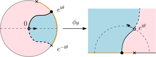
Figure 4: $C^{1}$ smooth geodesic pairs in $\mathbb{D}$ and $\mathbb{H}$.

Lemma 5.8.

The Schwarzian derivative of the uniformizing map $h_{\theta}\circ\phi_{\theta}^{-1}$ extends meromorphically with a simple pole at $z=e^{\mathfrak{i}\theta}$, and

$$C(h_{\theta}\circ\phi_{\theta}^{-1})(e^{\mathfrak{i}\theta})=\partial_{z}I_{\mathbb{H};0,\infty}(z)/2|_{z=e^{\mathfrak{i}\theta}}.$$

Proof.

It follows from Lemma 5.6 and Lemma 5.7 that

$$C(h_{\theta}\circ\phi_{\theta}^{-1})(e^{\mathfrak{i}\theta})=-\frac{4\cos\theta}{\phi^{\prime}_{\theta}(0)}=-\frac{2\cot\theta}{\mathfrak{i}e^{\mathfrak{i}\theta}}.$$

On the other hand, by Lemma 2.10,

$$I_{\mathbb{H};0,\infty}(z)=-8\log\frac{\operatorname{Im}z}{\left\lvert z\right\rvert}=-8\log\frac{z-\overline{z}}{2\mathfrak{i}}+4\log z\overline{z}.$$

We have

$$\partial_{z}I_{\mathbb{H};0,\infty}(z)|_{z=e^{\mathfrak{i}\theta}}=\frac{-8}{z-\overline{z}}+\frac{4}{z}\Big{|}_{z=e^{\mathfrak{i}\theta}}=\frac{-4(z+\overline{z})}{(z-\overline{z})z}\Big{|}_{z=e^{\mathfrak{i}\theta}}=\frac{-4\cot\theta}{\mathfrak{i}e^{\mathfrak{i}\theta}}=2C(h_{\theta}\circ\phi_{\theta}^{-1})(e^{\mathfrak{i}\theta})$$

as claimed. ∎

Proof of Theorem 5.5.

The Loewner chordal energy is conformally invariant, i.e., for $\psi:\mathbb{H}\to D$ a conformal map such that $a=\psi(0)$ and $b=\psi(\infty)$, we have $I_{D;a,b}(\psi(\gamma))=I_{\mathbb{H};0,\infty}(\gamma).$ Then we clearly have

$$I_{D;a,b}(\psi(z))=I_{\mathbb{H};0,\infty}(z).$$

This implies that $\partial_{z}I_{D;a,b}(z)$ also transforms like a $(1,0)$-form:

$$\partial_{z}I_{\mathbb{H};0,\infty}(z)=(\partial_{z}I_{D;a,b})\circ\psi(z)\cdot\psi^{\prime}(z),$$

with concludes the proof by Lemma 5.6 and Lemma 5.8. ∎

5.3 Schwarzian and the jump parameter

We now relate the residue $C$ in the Schwarzian to the parameter $\lambda$ of the jump of the pre-Schwarzian of the welding homeomorphism.

Let $\gamma$ be the $C^{1}$ smooth geodesic pair in $(D;a,b;z_{0})$, $\Omega$ the connected component of $D\smallsetminus\gamma$ where $(a,z_{0},b)$ are in counter-clockwise order in $\partial\Omega$, and $\Omega^{*}$ the connected component where $(a,z_{0},b)$ are in clockwise order of $\partial\Omega^{*}$. Let $f:\mathbb{H}\to\Omega$ and $g:\mathbb{H}^{*}\to\Omega^{*}$ be conformal maps such that the $x_{0}:=f^{-1}(z_{0})$ and $g^{-1}(z_{0})$ are not $\infty$. As before, we write the part of $\gamma$ from $a$ to $z_{0}$ as $\gamma_{1}$, and the part from $z_{0}$ to $b$ as $\gamma_{2}$.

Theorem 5.9.

The welding homeomorphism of $\gamma$, defined as $\varphi:=g^{-1}\circ f$ on the interval $f^{-1}(\gamma)\subset\hat{\mathbb{R}}$, is $C^{1}$, and in $\operatorname{PSL}(2,\mathbb{R})$ on $I_{1}:=f^{-1}(\gamma_{1})$ and on $I_{2}:=f^{-1}(\gamma_{2})$. Moreover, the jump $\lambda[\varphi](x_{0})$ of $\varphi^{\prime\prime}/\varphi^{\prime}$ at $\{x_{0}\}=I_{1}\cap I_{2}=\{f^{-1}(z_{0})\}$ satisfies

$$\frac{\lambda[\varphi](x_{0})}{f^{\prime}(x_{0})}=2\pi\mathfrak{i}\,C[f^{-1}](z_{0}).$$ (12)

Proof.

We consider first the case of a geodesic pair in $(\mathbb{D};e^{\mathfrak{i}\theta},e^{-\mathfrak{i}\theta};0)$, where $\theta\in(0,\pi/2]$ and choose $f=\mathfrak{f}_{\theta}$ and $g=\mathfrak{g}_{\theta}$ as defined in Section 2.5. Recall that by Lemma 2.18 we have

$$\lambda[\varphi_{\theta}](0)=-4\pi\cos(\theta).$$ (13)

and by Lemma 2.19 we also have

$$\mathfrak{f}_{\theta}^{\prime}(0)=(2\mathfrak{i})^{-1}.$$

On the other hand, $\mathfrak{f}_{\theta}^{-1}$ has the same Schwarzian as $h_{\theta}$, which was computed in Lemma 5.7. Hence by (13) we have

$$2\pi\mathfrak{i}C[\mathfrak{f}_{\theta}^{-1}](0)=-8\pi\mathfrak{i}\cos(\theta)=\frac{\lambda[\varphi_{\theta}](0)}{\mathfrak{f}_{\theta}^{\prime}(0)}.$$

Now we consider an arbitrary $C^{1}$ smooth geodesic pair in $(D;a,b;z_{0})$ and conformal maps $f:\mathbb{H}\to\Omega$ and $g:\mathbb{H}^{*}\to\Omega^{*}$. From the assumption, $f^{-1}(z_{0})=x_{0}\in\mathbb{R}$. We assume that $D$ is a simply connected domain conformally equivalent to $\mathbb{D}$ and $a\neq b$. Otherwise, we can cut open a piece of $\gamma_{1}$ near $a$, and the remaining curve is still a geodesic pair in the complement of the piece, and the corresponding welding is simply the restriction to a smaller interval containing $x_{0}$.

There exists $\theta\in(0,\pi/2]$ such that either $(D;a,b;z_{0})$ or $(D;b,a;z_{0})$ is conformally equivalent to $(\mathbb{D};e^{\mathfrak{i}\theta},e^{-\mathfrak{i}\theta};0)$. Assume without loss of generality that $(D;a,b;z_{0})$ is conformally equivalent to $(\mathbb{D};e^{\mathfrak{i}\theta},e^{-\mathfrak{i}\theta};0)$ by a conformal map $\psi:\mathbb{D}\to D$ respecting the marked points (otherwise, we switch $f$ and $g$ and replace $\varphi$ by $\varphi^{-1}$).

Now let $\alpha\in\operatorname{PSL}(2,\mathbb{R})$ such that $f=\psi\circ\mathfrak{f}_{\theta}\circ\alpha$. In particular, $\alpha(x_{0})=0$. Similarly, let $\beta\in\operatorname{PSL}(2,\mathbb{R})$ such that $g=\psi\circ\mathfrak{g}_{\theta}\circ\beta$. The assumption that $g^{-1}(z_{0})=:y_{0}\neq\infty$ implies that $\beta(y_{0})=0$ and $\beta^{-1}$ is regular near $0$. We obtain

$$\varphi=\beta^{-1}\circ\varphi_{\theta}\circ\alpha.$$

Using the chain rules

$$\lambda[\varphi](x_{0})=\lambda[\varphi_{\theta}](0)\alpha^{\prime}(x_{0}),\qquad f^{\prime}(x_{0})=\psi^{\prime}(0)\mathfrak{f}_{\theta}^{\prime}(0)\alpha^{\prime}(x_{0})$$

and

$$C[f^{-1}](z_{0})=C[\mathfrak{f}_{\theta}^{-1}\circ\psi^{-1}](z_{0})=\frac{C[\mathfrak{f}_{\theta}^{-1}](0)}{\psi^{\prime}(0)},$$

we obtain

$$\frac{\lambda[\varphi](x_{0})}{f^{\prime}(x_{0})}=\frac{\lambda[\varphi_{\theta}](0)}{\psi^{\prime}(0)f_{\theta}^{\prime}(0)}=2\pi\mathfrak{i}\frac{C[\mathfrak{f}_{\theta}^{-1}](0)}{\psi^{\prime}(0)}=2\pi\mathfrak{i}C[f^{-1}](z_{0})$$

which completes the proof. ∎

5.4 Schwarzian and piecewise geodesic Jordan curve

We fix an isotopy class $\mathcal{L}(z_{1},\ldots,z_{n};\tau)$. Let $\gamma$ be the unique piecewise geodesic Jordan curve in this class and define $I(z_{1},\ldots,z_{n};\tau)=I^{L}(\gamma)$. As before, we write $\gamma\smallsetminus\{z_{1},\dots,z_{n}\}=\gamma_{1}\cup\ldots\cup\gamma_{n}$ where $\gamma_{k}$ connects $z_{k}$ to $z_{k+1}$, and $\Omega_{+}$ (resp. $\Omega_{-}$) for the connected component of $\widehat{\mathbb{C}}\smallsetminus\gamma$ where the marked points are ordered counterclockwise (resp. clockwise) on the boundary. For small enough $\varepsilon>0$, the ball $B_{\varepsilon}(z_{k})$ of Euclidean radius $\varepsilon$ centered at $z_{k}$ does not intersect $\gamma\smallsetminus(\gamma_{k-1}\cup\gamma_{k}\cup\{z_{k}\})$. For $z\in B_{\varepsilon}(z_{k})$, we write $\gamma^{z}_{k}$ for the unique $C^{1}$ smooth geodesic pair in $(\Omega_{+}\cup\Omega_{-}\cup\gamma_{k-1}\cup\gamma_{k}\cup\{z_{k}\};z_{k-1},z_{k+1};z)$. We define $I(z_{1},\ldots,z_{k-1},z,z_{k+1},\ldots z_{n};\tau)$ to be the minimal energy of Jordan curves isotopic to $(\gamma\smallsetminus\gamma^{z_{k}}_{k})\cup\gamma^{z}_{k}$.

Theorem 5.10.

Let $Z_{\gamma}$ be the associated projective structure defined in Section 5.1 and $q$ the corresponding quadratic differential defined in Lemma 2.3. Assume that $z_{k}\neq\infty$ for all $k=1,\ldots,n$. We have

$$q(w)=\sum_{k=1}^{n}\frac{\partial_{k}I(z_{1},\ldots,z_{n};\tau)/2}{w-z_{k}}\,\mathrm{d}w^{2},$$

where $\partial_{k}=(\partial_{x_{k}}-\mathfrak{i}\partial_{y_{k}})/2$ if $z_{k}=x_{k}+\mathfrak{i}y_{k}$.

Remark 5.11.

Let us first make a few remarks.

• If we normalize the $n$-punctured sphere such that $z_{n-2}=0$, $z_{n-1}=1$, and $z_{n}=\infty$, then the expression of $q$ can be easily obtained using the property of quadratic differentials, see (4). The assumption of $\infty$ not being a marked point makes the expression of $q$ cleaner, so we only consider this case.

• This result is very similar to the result on the accessory parameter of the Fuchsian projective structure, first conjectured by Polyakov and proved by Takhtajan and Zograf in [28, Thm. 1], which shows that the associated quadratic differential is given by

  $$q_{F}(w)=\sum_{k=1}^{n}\left(\frac{1}{2(w-z_{k})^{2}}-\frac{\partial_{k}S_{cl}}{2\pi}\frac{1}{(w-z_{k})}\right)\,\mathrm{d}w^{2}$$

  where $S_{cl}$ is the classical Liouville action on the $n$-punctured sphere.

• Note that $q$ also uniquely determines $\gamma$. In fact, if $q_{j}$, $j=1,2$, is the quadratic differential associated with a piecewise geodesic Jordan curve $\gamma_{j}$ and if $q_{1}=q_{2}$, then Lemma 2.3 shows that $Z_{\gamma_{1}}=Z_{\gamma_{2}}$. In particular, there exists $A\in\operatorname{PSL}(2,\mathbb{C})$ such that $h_{1}=A\circ h_{2}$, where $h_{j}$ is the developing map with the holonomy representation in $\operatorname{PSL}(2,\mathbb{R})$. As any lift $h_{j}\circ\Pi^{-1}|_{\Omega_{j,+}}$ maps $\Omega_{j,+}$ to $\mathbb{R}$ and the marked points into $\widehat{\mathbb{R}}$, as $n\geq 3$, $A$ has to map at least $3$ points on $\widehat{\mathbb{R}}$ into $\widehat{\mathbb{R}}$, hence $A\in\operatorname{PSL}(2,\mathbb{R})$. Since $\gamma_{j}=\Pi\circ h_{j}^{-1}(\widehat{\mathbb{R}})$ and $h_{1}^{-1}(\widehat{\mathbb{R}})=h_{2}^{-1}\circ A^{-1}(\widehat{\mathbb{R}})=h_{2}^{-1}(\widehat{\mathbb{R}})$, we obtain $\gamma_{1}=\gamma_{2}$.

Proposition 5.12.

The function

$$I(\cdot;\tau)\colon(z_{1},\ldots,z_{n})\mapsto I(z_{1},\ldots,z_{n};\tau)$$

is $C^{1}$ smooth and for all $k=1,\cdots,n$,

$$\partial_{z_{k}}I(z_{1},\ldots,z_{n};\tau)=\partial_{z}I_{D_{k};z_{k-1},z_{k+1}}(z_{k}),$$

where $D_{k}=\Omega_{+}\cup\Omega_{-}\cup\gamma^{z_{k}}_{k}$ and $I_{D_{k};z_{k-1},z_{k+1}}(z)=I_{D_{k};z_{k-1},z_{k+1}}(\gamma^{z}_{k})$.

Proof.

We first notice that if $I(z_{1},\ldots,z_{n};\tau)$ is differentiable at $z_{k}$, then

$$\partial_{z_{k}}I(z_{1},\ldots,z_{n};\tau)=\partial_{z}I_{D_{k};z_{k-1},z_{k+1}}(z_{k}),$$ (14)

since by definition,

$$I(z_{1},\ldots,z_{k-1},\cdot,z_{k+1},\ldots,z_{n};\tau)\leq I_{D_{k};z_{k-1},z_{k+1}}(\cdot)+I^{A}(\gamma\smallsetminus\gamma^{z_{k}}_{k})$$

and they coincide at $z_{k}$.

To show the differentiability, we show first that $I(z_{1},\ldots,z_{k-1},\cdot,z_{k+1},\ldots,z_{n};\tau)$ is locally Lipschitz. From Theorem 4.4, the unique piecewise geodesic Jordan curve $\gamma^{z_{k}}$ in $\mathcal{L}(z_{1},\cdots,z_{n};\tau)$ depends continuously on $z_{k}$ with respect to the Hausdorff metric. Therefore for every $z_{k}$, there exist a ball $B_{r}(z_{k})$ with some radius $r>0$ centered at $z_{k}$, such that for all $z\in B_{r}(z_{k})$, we have $B_{2r}(z_{k})\cap\hat{\gamma}^{z}=\emptyset$ where $\hat{\gamma}^{z}$ is the arc in $\gamma^{z}$ obtained by removing the geodesic pair passing through $z$. In particular, this implies that the image of $B_{r}(z_{k})$ under the conformal map $h_{z}:\widehat{\mathbb{C}}\smallsetminus\hat{\gamma}^{z}\to\mathbb{H}$ sending $z_{k-1}\mapsto 0$, $z_{k+1}\mapsto\infty$, $z\mapsto e^{\mathfrak{i}\theta}$ for some $\theta$, is contained in a compact set $K\subset\mathbb{H}$ (which is independent of $z\in B_{r}(z_{k})$).

Therefore, for $z,z^{\prime}\in B_{r}(z_{k})$,

$$I(z_{1},\ldots,z_{k-1},z^{\prime},z_{k+1},\ldots,z_{n};\tau)-I(z_{1},\ldots,z_{k-1},z,z_{k+1},\ldots,z_{n};\tau)$$

$$\leq I^{A}(\hat{\gamma}^{z})+I_{\widehat{\mathbb{C}}\smallsetminus\hat{\gamma}^{z};z_{k-1},z_{k+1}}(z^{\prime})-I(z_{1},\ldots,z_{k-1},z,z_{k+1},\ldots z_{n};\tau)$$

$$=I_{\mathbb{H};0,\infty}(h_{z}(z^{\prime}))-I_{\mathbb{H};0,\infty}(h_{z}(z)).$$

Since $h_{z}(z^{\prime}),h_{z}(z)\in K$, $I_{\mathbb{H};0,\infty}(\cdot)$ is smooth in $K$ and $h_{z}^{\prime}$ is uniformly bounded in $B_{r}(z_{k})$ for all $z\in B_{r}(z_{k})$, we obtain that there exists $c=c(z_{k},r)$ such that for all $z,z^{\prime}\in B_{r}(z_{k})$,

$$I(z_{1},\ldots,z_{k-1},z^{\prime},z_{k+1},\ldots,z_{n};\tau)-I(z_{1},\ldots,z_{k-1},z,z_{k+1},\ldots,z_{n};\tau)\leq c|z^{\prime}-z|.$$

This proves that $I(\cdot;\tau)$ is locally Lipschitz.

From the Rademacher theorem, the Lipschitz function $I(\cdot;\tau)$ is differentiable almost everywhere. Let $(z_{1},\ldots,z_{k-1},z_{k},z_{k+1},\ldots,z_{n})$ be a differentiable point of $I(\cdot;\tau)$. Let $\gamma$ be the unique minimizer in the isotopy class $(z_{1},\ldots,z_{k-1},z_{k},z_{k+1},\ldots,z_{n};\tau)$, and let $f:\mathbb{H}\to\Omega$ and $g:\mathbb{H}^{*}\to\Omega^{*}$ be two conformal maps as before. We parametrize the welding homeomorphism $\varphi=g^{-1}\circ f$ by the coordinates $(x_{k},\lambda_{k}=\lambda[\varphi](x_{k}))$ as in Section 4. We have for all $k=1,\cdots,n$,

$$\partial_{z_{k}}I(z_{1},\ldots,z_{n};\tau)=\partial_{z}I_{D_{k};z_{k-1},z_{k+1}}(z_{k})=2C[f^{-1}](z_{k})=\frac{\lambda_{k}}{\pi\mathfrak{i}f^{\prime}(x_{k})}.$$

The first equality follows from the observation (14), the second equality follows from Theorem 5.5, and the last equality follows from Theorem 5.9.

Recalling the factorization $f=\psi\circ\mathfrak{f}_{\theta}\circ\alpha$ from Lemma 4.6 we see that $f^{\prime}(x_{k})=\frac{1}{2\mathfrak{i}}\psi^{\prime}(0)\alpha^{\prime}(x_{k})$, which is a continuous function of $p\in\mathcal{W}_{n}$. Hence $\lambda_{k}/f^{\prime}(x_{k})$ depends continuously on $(z_{1},\cdots,z_{n})$. Thus the almost everywhere defined partial derivatives of $I(\cdot;\tau)$ extend to continuous functions. As $I(\cdot;\tau)$ is absolutely continuous on lines, it is determined by its partial derivatives and hence is a $C^{1}$ function, which completes the proof. ∎

Proof of Theorem 5.10.

Recall that the quadratic differential $q$ is defined as $\mathcal{S}[h\circ\pi^{-1}]$. Here, $h:\tilde{\Sigma}\to\widehat{\mathbb{C}}$ is a developing map constructed in Section 5.1 such that any lift of $h\circ\pi^{-1}$ restricted to $\Omega_{+}$, is a conformal map from $\Omega_{+}$ onto $\mathbb{H}$. Since for all $1\leq k\leq n$, $\gamma^{z_{k}}_{k}=\gamma_{k-1}\cup\gamma_{k}\cup\{z_{k}\}$ is a geodesic pair in $(D_{k};z_{k-1},z_{k+1})$, Theorem 5.5 and Proposition 5.12 show that

$$q(w)\sim\frac{\partial_{z}I_{D_{k};z_{k-1},z_{k+1}}(z_{k})/2}{w-z_{k}}=\frac{\partial_{k}I(z_{1},\ldots z_{n};\tau)/2}{w-z_{k}},\qquad\text{as }w\to z_{k}.$$

As $q$ does not have a pole at $\infty$, as a Schwarzian derivative, it means that

$$q(w)=O(w^{-4})\qquad\text{as }w\to\infty.$$

We obtain the claimed expression of $q$ since the difference of the left- and right-hand sides is holomorphic on $\widehat{\mathbb{C}}$ and vanishes as $w\to\infty$. ∎

6 Relation to Fuchsian projective structures

In this section, we will show how one can obtain piecewise geodesic Jordan curves and their associated projective structures by grafting the Fuchsian projective structures.

We first notice that there is another natural way to associate a unique Jordan curve in an isotopy class $\mathcal{L}(w_{1},\ldots,w_{n};\tau)$ with a marked Fuchsian projective structure, which gives another parametrization of $T_{0,n}$ by Jordan curves.

Lemma 6.1.

Let $w_{1},\ldots,w_{n}\in\widehat{\mathbb{C}}$, $n\geq 3$, be distinct points, $\tau$ be a Jordan curve passing through $w_{1},\ldots,w_{n}$ in cyclic order, and $\Sigma^{\prime}\coloneqq\widehat{\mathbb{C}}\smallsetminus\{w_{1},\dots,w_{n}\}$ be the $n$-punctured sphere endowed with its complete hyperbolic metric. Then in the isotopy class $\mathcal{L}(w_{1},\ldots,w_{n};\tau)$ there exists a unique Jordan curve $\gamma^{\prime}$ such that each arc of $\gamma^{\prime}$ between consecutive cusps is a hyperbolic geodesic in $\Sigma^{\prime}$.

Proof.

We denote by $\Pi^{\prime}\colon\mathbb{H}\to\Sigma^{\prime}$ the (essentially unique) holomorphic universal covering map and by $\Gamma^{\prime}\subset\operatorname{PSL}(2,\mathbb{R})$ the group of deck transformations. The preimage of $\tau$ by $\Pi^{\prime}$ (see Figure 3) is a union of disjoint chords in $\mathbb{H}$ invariant under $\Gamma^{\prime}$. We now replace each chord with the hyperbolic geodesic in $\mathbb{H}$ with the same endpoints. In this way we get a $\Gamma^{\prime}$-invariant family of hyperbolic geodesics. No pair of these geodesics can cross, because this would lead to a corresponding crossing of the chords arising from $\tau$. This implies that the images of these geodesics under $\Pi^{\prime}$ with the cusps in $\Sigma^{\prime}$ added give a Jordan curve $\gamma^{\prime}$. It is easy to see that this the unique Jordan curve sought after. ∎

In [12, Lem. 4.2], it was shown that $\gamma^{\prime}$ is different from the unique curve in $\mathcal{L}(w_{1},\ldots,w_{n};\tau)$ with the geodesic property discussed in the rest of the paper, except when $\gamma^{\prime}$ is a circle. We now show that their corresponding projective structures are related by a $\pi$-angle grafting.

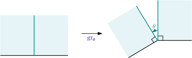
Figure 5: Grafting by $\theta$ along $\mathfrak{i}\mathbb{R}_{+}$.

Grafting is a way to deform a Riemann surface by inserting a new space along a measured lamination (see, e.g., [8, 22]). In the simplest case, grafting by an angle $\theta>0$ along the imaginary axis in the upper half-plane model can be defined by constructing a Riemann surface where one inserts a wedge of angle $\theta$ at the origin as in Figure 5. Grafting along other geodesics in $\mathbb{H}$ can always be reduced to this case by conjugating by a Möbius transformation. Grafting along a geodesic on a general hyperbolic surface is realized in such a way that it lifts to the grafting along all the lifts of the geodesic on the universal cover $\mathbb{H}$. Grafting also defines a projective structure on the resulting surface, since locally the construction takes place on the Riemann sphere and defines a developing map in a natural way.

We will only consider grafting along countably many geodesics by the angle $\theta=\pi$ where the inserted wedge is a half-plane, or in the case where we graft along a semicircle and the inserted region becomes a disc, see Figure 6.

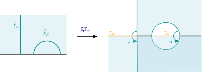
Figure 6: Grafting by $\pi$ along two geodesics $\alpha$ and $\beta$.

Let $\gamma^{\prime}$ be a Jordan curve as in Lemma 6.1. Let $\gamma_{k}^{\prime}$ be the geodesic on $\Sigma^{\prime}$ between $w_{k}$ and $w_{k+1}$ (which is part of $\gamma^{\prime}$) and $\Pi^{\prime}:\mathbb{H}\to\Sigma^{\prime}$ be a covering map. Let $\tilde{\Sigma}$ be the Riemann surface obtained by grafting along all lifts $\tilde{\ell}_{\alpha}$ of the geodesics $\gamma_{k}^{\prime}$ ($k=1,\dots,n$), inserting a $\pi$-angle wedge $\tilde{V}_{\alpha}$. Let $\Sigma=\widehat{\mathbb{C}}\smallsetminus\{z_{1},\ldots,z_{n}\}$ be the corresponding $n$-punctured Riemann surface obtained by grafting into each $\gamma_{k}^{\prime}$ a $\pi$-angle wedge $V_{k}$. This way, we obtain a covering map $\Pi:\tilde{\Sigma}\to\Sigma$. We denote by $\tilde{\gamma}_{\alpha}$ the central line of $\tilde{V}_{\alpha}$ and $\gamma_{k}$ the central line of $V_{k}$, so that the image of $\tilde{\gamma}_{\alpha}$ under $\Pi$ is one of $\{\gamma_{1},\ldots,\gamma_{n}\}$. See Figure 7 illustrating the grafting map on a $4$-punctured sphere.

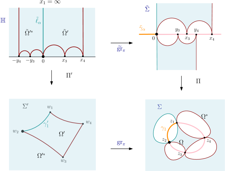
Figure 7: Illustration of the grafting by $\pi$ along the geodesics $\gamma^{\prime}_{k}$ on a $4$-punctured sphere $\Sigma^{\prime}$, for $k=1,\ldots,4$, in a local chart.

Proposition 6.2.

The central lines $\tilde{\gamma}_{\alpha}$ form a graph $\tilde{G}$ on $\tilde{\Sigma}$ with geodesic property. In particular, this implies that the Jordan curve $\gamma:=\gamma_{1}\cup\cdots\cup\gamma_{n}$ formed by the union of the central lines of $(V_{k})_{k=1,\ldots,n}$ has the geodesic property. Moreover, the welding homeomorphism of $\gamma$ is $C^{1}$ smooth, and the inverse of $\Pi$ is a projective chart of the projective structure associated with $\gamma$ as in Section 5.1. It has a holonomy representation given by

$$\rho_{\gamma}(\eta_{k})=S_{k-1}\circ\rho_{F}(\eta_{k}^{\prime})\circ S_{k},$$ (15)

where $\rho_{F}$ is a holonomy representation of the uniformizing structure on $\Sigma^{\prime}$, $\eta_{k}$ and $\eta_{k}^{\prime}$ are the standard generators of $\pi_{1}(\Sigma)$ and $\pi_{1}(\Sigma^{\prime})$, respectively, and $S_{k}$ is the Möbius transform that rotates by angle $\pi$ around the two fixed points $x_{k}$ and $x_{k+1}$ of $\rho_{F}(\eta_{k}^{\prime})$ and $\rho_{F}(\eta_{k+1}^{\prime})$, respectively.

Proof.

Let $\tilde{\ell}_{\alpha}\subset\mathbb{H}$ be a lift of the geodesic $\gamma_{1}^{\prime}$ (the same proof works for $\gamma_{k}^{\prime}$). We now check that the corresponding central line $\tilde{\gamma}_{\alpha}$ is the hyperbolic geodesic in the union of the two adjacent faces of $\tilde{G}$. Without loss of generality, we assume that $\tilde{\ell}_{\alpha}=\mathfrak{i}\mathbb{R}_{+}$, and the covering map $\Pi^{\prime}$ maps $\infty$ to $w_{1}$ and $0$ to $w_{2}$. A fundamental domain of $\Pi^{\prime}$ is given by a union of two ideal $n$-gons $\tilde{\Omega}^{\prime}$ and $\tilde{\Omega}^{\prime*}$ with $\mathfrak{i}\mathbb{R}_{+}$ being one of the edges. See Figure 7. It is immediate that after grafting by $\pi$ along all the edges of $\tilde{\Omega}^{\prime}$ and $\tilde{\Omega}^{\prime*}$, the central line $\tilde{\gamma}_{\alpha}$ obtained is $\mathbb{R}_{-}$, and the union of the central lines associated with the other edges of $\tilde{\Omega}^{\prime}$ (resp. of $\tilde{\Omega}^{\prime*}$) is $\mathbb{R}_{+}$. Since $\mathbb{R}_{-}$ is the hyperbolic geodesic of $\mathbb{C}\smallsetminus\mathbb{R}_{+}$, this shows the geodesic property of $\tilde{G}$.

In the local chart $\mathbb{C}\smallsetminus\mathbb{R}_{-}$ around $\tilde{\gamma}_{\alpha}=\mathbb{R}_{-}$, the covering map $\Pi:\tilde{\Sigma}\to\Sigma$ maps respectively the upper and lower halfplanes to the two connected components of $\widehat{\mathbb{C}}\smallsetminus\gamma$. This shows that $\gamma_{1}$ is also a hyperbolic geodesic of the simply connected domain $\widehat{\mathbb{C}}\smallsetminus(\cup_{k\geq 2}\gamma_{k})$, proving the geodesic property of $\gamma$.

Now we show that the welding homeomorphism of $\gamma$ is $C^{1}$. Notice that in the local chart illustrated in Figure 7, we may already read a welding homeomorphism $\varphi$ of $\gamma$. Indeed, we can write $\varphi:=\Pi_{-}^{-1}\circ\Pi_{+}|_{\widehat{\mathbb{R}}}$, where $\Pi_{+}=\Pi|_{\mathbb{H}}$ and $\Pi_{-}=\Pi|_{\mathbb{H}^{*}}$ and in this chart $\Pi$ is continuous along $\tilde{\gamma}_{\alpha}=\mathbb{R}_{-}$, so that $\varphi|_{\mathbb{R}_{-}}$ is the identity map. We also notice that $\varphi(x_{k})=y_{k}$ for $k=3,\ldots,n.$ By Proposition 5.2, $\varphi|_{[0,x_{3}]}$ is given by the holonomy $\rho_{\gamma}(\eta_{2})\in\operatorname{PSL}(2,\mathbb{R})$ around $z_{2}$, which is of the form $\rho_{\gamma}(\eta_{2})=S_{1}\circ\rho_{F}(\eta_{2}^{\prime})\circ S_{2}$. Here, $\rho_{F}(\eta_{2}^{\prime})\in\operatorname{PSL}(2,\mathbb{R})$ is the holonomy around $w_{2}$ for the Fuchsian projective structure which is parabolic and fixes $0$, $S_{1}(z)=-z$ realizes the $\pi$-grafting along $\tilde{\ell}_{\alpha}=\mathfrak{i}\mathbb{R}_{+}$, and $S_{2}$ realizes the $\pi$-grafting along the geodesic passing through $0$ and $x_{3}$ (which is a conjugate of $S_{1}$). In particular, both $S_{1}$ and $S_{2}$ have derivative $-1$ at $0$. We obtain that $\rho(\eta_{2})^{\prime}(0)=1$. This shows that $\varphi^{\prime}$ is continuous at $0$. Similarly, if $S_{k}$ realizes the $\pi$-grafting along the geodesic between $x_{k}$ and $x_{k+1}$, we see that $\rho_{\gamma}(\eta_{k})=S_{k-1}\circ\rho_{F}(\eta_{k})\circ S_{k}$ is parabolic, and by Proposition 5.2 and induction we have

$$\varphi|_{[x_{k},x_{k+1}]}=\rho_{\gamma}(\eta_{2})\circ\dots\circ\rho_{\gamma}(\eta_{k}).$$ (16)

This completes the proof. ∎

Proposition 6.2 shows that from a marked Fuchsian projective structure and its unique geodesic Jordan curve $\gamma^{\prime}$, the $\pi$-angle grafting along all the arcs of $\gamma^{\prime}$ gives the projective structure associated with a Jordan curve with the geodesic property. Projecting down to $T_{0,n}$, we obtain a map $\operatorname{gr}_{\pi}:T_{0,n}\to T_{0,n}$.

Corollary 6.3.

The map $\operatorname{gr}_{\pi}$ is a differentiable bijection $T_{0,n}\to T_{0,n}$.

Proof.

We first show that $\operatorname{gr}_{\pi}$ is bijective by identifying its inverse, namely, a de-grafting map.

Let $\mathcal{L}(z_{1},\ldots,z_{n};\tau)$ be an isotopy class of Jordan curves representing a point in $T_{0,n}$. Theorem 3.1 shows that there exists a unique Jordan curve $\gamma=\gamma_{1}\cup\cdots\cup\gamma_{n}$ in $\mathcal{L}(z_{1},\ldots,z_{n};\tau)$ with the geodesic property. Let $\Omega$ and $\Omega^{*}$ denote the two connected components of $\widehat{\mathbb{C}}\smallsetminus\gamma$.

From the construction of the projective structure associated with $\gamma$ in Section 5.1, there is a projective chart $H:\Omega\cup\Omega^{*}\cup\gamma_{1}\to\mathbb{H}\cup\mathbb{H}^{*}\cup\mathbb{R}_{-}$, such that $H(\gamma_{1})=\mathbb{R}_{-}$. We note that $H$ coincides with $\Pi^{-1}$ in the local chart shown in Figure 7. Let $V_{1}$ denote $H^{-1}(\{z\colon\operatorname{Re}(z)<0\})$ and similarly $V_{k}$ for all $k=2,\ldots,n$. We note that $\partial V_{1}\cap\Omega$ is a hyperbolic geodesic in $\Omega$. This implies that $V_{k}$ are pairwise disjoint. Let $V=\cup_{k=1}^{n}V_{k}$.

We let $\Sigma^{\prime}=\widehat{\mathbb{C}}\smallsetminus\{w_{1},\ldots,w_{n}\}$ be the Riemann surface obtained by identifying $\partial V_{k}\cap\Omega$ with $\partial V_{k}\cap\Omega^{*}$ such that in the chart $H$, $\mathfrak{i}x$ is identified with $-\mathfrak{i}x$. We modify the projective chart by degrafting by $\pi$, so that the new chart is given by

$$H^{\prime}(z)=\begin{cases}H(z),\quad&z\in\Omega\smallsetminus V\\ -H(z),&z\in\Omega^{*}\smallsetminus V.\end{cases}$$

In particular, it takes value in $\tilde{\Omega}^{\prime}\cup\tilde{\Omega}^{\prime*}\subset\mathbb{H}$, where $\tilde{\Omega}^{\prime}$ and $\tilde{\Omega}^{\prime*}$ are illustrated in Figure 7. By induction, the analytic continuation $\tilde{H}$ of $H$ to the universal cover of $\Sigma^{\prime}$ takes value in $\mathbb{H}$ and is injective. The same argument as in the proof of Proposition 6.2 shows that the holonomy associated with the projective structure on $\Sigma^{\prime}$ is parabolic and in $\operatorname{PSL}(2,\mathbb{R})$ around each puncture. Therefore, $H$ defines a hyperbolic metric on $\Sigma^{\prime}$ by pulling back the metric on $\mathbb{H}$ for which the arcs of $\gamma^{\prime}$ are geodesics (as the holonomies are isometries of $\mathbb{H}$).

Moreover, the parabolic holonomy around $w_{k}$ implies that there is a neighborhood of $w_{k}$ that is isometric to a cusp for all $k$. Hence, $\Sigma^{\prime}$ is complete. We deduce that $\tilde{H}$ is surjective onto $\mathbb{H}$ and defines a Fuchsian projective structure on $\Sigma^{\prime}$.

To see that $\operatorname{gr}_{\pi}$ is differentiable, we note that by [28, Lemma 3] the (multi-valued) map $(w_{1},\dots,w_{n})\mapsto\rho_{F}$ is complex analytic, while $\rho_{F}\mapsto\rho_{\gamma}$ is differentiable by the explicit formula (15), $\rho_{\gamma}\mapsto\varphi$ is differentiable by formula (16) and finally $\varphi\mapsto(z_{1},\dots,z_{n})$ is differentiable by Theorem 4.4. ∎

Let us end by making a few comments about connections to existing literature. In [18], it is shown that grafting laminations of (limits of) simple closed geodesics gives a self-homeomorphism of the Teichmüller space. We have thus given an example where the same result holds for a lamination consisting of open geodesics connecting punctures. It would be interesting to see whether our methods could be generalized to more general half-integral laminations, a question that has also appeared in the context of the analytic Langlands program in [7, Appendix A1]. Such laminations are closely related to projective structures with real holonomy, which in general can also include extra data such as the spiraling rate of a logarithmic spiral at a given puncture. In the grafting construction, spiraling would correspond to adding an earthquake to the grafting.

Acknowledgments: We thank Peter Lin, Donald Marshall, and Curtis McMullen for helpful discussions. M.B. is supported by NSF grant DMS-1808856. J.J. is supported by The Finnish Centre of Excellence (CoE) in Randomness and Structures. S.R. is supported by NSF Grants DMS-1954674 and DMS-2350481. Y.W. is supported by the European Union (ERC, RaConTeich, 101116694). This work is also supported by NSF Grant DMS-1928930 while the authors participated in a program hosted by the Mathematical Sciences Research Institute in Berkeley, California, during the Spring 2022 semester.

References

- [1] C. J. Bishop. Weil–Petersson curves, -numbers, and minimal surfaces. Annals of Math., to appear.
- [2] M. Bonk and A. Eremenko. Canonical embeddings of pairs of arcs. Comput. Methods Funct. Theory, 21(4):825–830, 2021.
- [3] M. Bridgeman, K. Bromberg, F. Vargas-Pallete, and Y. Wang. Universal Liouville action as a renormalized volume and its gradient flow. Preprint, arXiv:2311.18767, 2023.
- [4] G. Cui. Integrably asymptotic affine homeomorphisms of the circle and Teichmüller spaces. Sci. China Ser. A, 43(3):267–279, 2000.
- [5] M. L. de Cristoforis and L. Preciso. Differentiability properties of some nonlinear operators associated to the conformal welding of Jordan curves in schauder spaces. Hiroshima Math. J., 33(1):59–86, 2003.
- [6] D. Dumas. Complex projective structures. In Handbook of Teichmüller theory. Vol. II, volume 13 of IRMA Lect. Math. Theor. Phys., pages 455–508. Eur. Math. Soc., Zürich, 2009.
- [7] D. Gaiotto and J. Teschner. Quantum analytic langlands correspondence. Preprint, arXiv:2402.00494, 2024.
- [8] W. M. Goldman. Projective structures with fuchsian holonomy. J. Dff. Geom., 25(3):297–326, 1987.
- [9] K. Johansson. Strong Szegö theorem on a Jordan curve. In Toeplitz operators and random matrices—in memory of Harold Widom, volume 289 of Oper. Theory Adv. Appl., pages 427–461. Birkhäuser/Springer, Cham, 2022.
- [10] K. Johansson and F. Viklund. Coulomb gas and the Grunsky operator on a Jordan domain with corners. Preprint, arXiv:2309.00308, 2023.
- [11] O. Lehto. Univalent functions and Teichmüller spaces, volume 109 of Graduate Texts in Mathematics. Springer, New York, 1987.
- [12] D. Marshall, S. Rohde, and Y. Wang. Piecewise geodesic Jordan curves I: weldings, explicit computations, and Schwarzian derivatives. Preprint, arXiv:2202.01967, 2022.
- [13] C. T. McMullen. Complex earthquakes and Teichmüller theory. J. Amer. Math. Soc., 11(2):283–320, 1998.
- [14] T. Mesikepp. A deterministic approach to Loewner-energy minimizers. Math. Z., 305(4), 2023.
- [15] E. Peltola and Y. Wang. Large deviations of multichordal , real rational functions, and zeta-regularized determinants of Laplacians. J. Eur. Math. Soc. (JEMS), 26(2):469–535, 2024.
- [16] C. Pommerenke. Boundary behaviour of conformal maps, volume 299 of Grundlehren der Mathematischen Wissenschaften. Springer, Berlin, 1992.
- [17] S. Rohde and Y. Wang. The Loewner energy of loops and regularity of driving functions. Int. Math. Res. Not., 2021(10):7715–7763, 2021.
- [18] K. Scannell and M. Wolf. The grafting map of Teichmüller space. J. Amer. Math. Soc., 15(4):893–927, 2002.
- [19] Y. Shen. Weil-Petersson Teichmüller space. Amer. J. Math., 140(4):1041–1074, 2018.
- [20] L. Takhtajan and P. Zograf. Hyperbolic 2-spheres with conical singularities, accessory parameters and Kähler metrics on . Trans. Amer. Math. Soc., 355(5):1857–1867, 2003.
- [21] L. A. Takhtajan and L.-P. Teo. Weil-Petersson metric on the universal Teichmüller space. Mem. Amer. Math. Soc., 183(861), 2006.
- [22] H. Tanigawa. Grafting, harmonic maps and projective structures on surfaces. J. Diff. Geom., 47(3):399–419, 1997.
- [23] Y. Wang. The energy of a deterministic Loewner chain: reversibility and interpretation via . J. Eur. Math. Soc., 21(7):1915–1941, 2019.
- [24] Y. Wang. Equivalent descriptions of the Loewner energy. Invent. Math., 218(2):573–621, 2019.
- [25] Y. Wang. A note on Loewner energy, conformal restriction and Werner’s measure on self-avoiding loops. Ann. Inst. Fourier (Grenoble), 71(4):1791–1805, 2021.
- [26] Y. Wang. Two optimization problems for the Loewner energy, 2024. Preprint, arXiv:2402.10054, 2024.
- [27] C. Wong. Smoothness of Loewner slits. Trans. Amer. Math. Soc., 366(3):1475–1496, 2014.
- [28] P. G. Zograf and L. A. Takhtadzhyan. On the Liouville equation, accessory parameters and the geometry of Teichmüller space for Riemann surfaces of genus . Mat. Sbornik (N.S.), 132(174)(2):147–166, 1987.