Fourier Head:
Helping Large Language Models
Learn Complex Probability Distributions

Abstract

As the quality of large language models has improved, there has been increased interest in using them to model non-linguistic tokens. For example, the Decision Transformer recasts agentic decision making as a sequence modeling problem, using a decoder-only LLM to model the distribution over the discrete action space for an Atari agent. However, when adapting LLMs to non-linguistic domains, it remains unclear if softmax over discrete bins captures the continuous structure of the tokens and the potentially complex distributions needed for high quality token generation. We introduce a neural network layer, constructed using Fourier series, which we can easily substitute for any linear layer if we want the outputs to have a more continuous structure. We perform extensive analysis on synthetic datasets, as well as on large-scale decision making and time series forecasting tasks. We also provide theoretical evidence that this layer can better learn signal from data while ignoring high-frequency noise. All of our results support the effectiveness of our proposed Fourier head in scenarios where the underlying data distribution has a natural continuous structure. For example, the Fourier head improves a Decision Transformer agent’s returns by 46% on the Atari Seaquest game, and increases a state-of-the-art times series foundation model’s forecasting performance by 3.5% across 20 benchmarks unseen during training. We release our implementation at https://nategillman.com/fourier-head.

Fourier Head Learns Higher Quality Densities

Figure 1: We task an MLP with learning to approximate a continuous bimodal density using a categorical distribution and a cross entropy objective. We observe that a standard linear classification head fails to distinguish between the two modes, and overfits to high-frequency noise in the training set. In contrast, our proposed Fourier head learns a smoother, more accurate categorical distribution.

1 Introduction

Human language can be viewed as a discretization for a continuous, often probabilistic representation of the world that is construed in our mind (Spivey, 2008). The continuous structure can be partially captured by language models with their token embeddings, where “nearby” tokens are embedded to have latent representations with high cosine similarities. The embeddings themselves are acquired as a result of the data-driven learning process. Can we, based on rich prior knowledge about the continuous world, inform the language model about the underlying continuity of its inputs, like the fact that the word “emerald” is more similar to “shamrock” than “pine” when they are used to describe different shades of green? As large language models (LLMs) have evolved into “foundation models” that are adapted to a diverse range of tasks, tokens that are a priori continuous are more essential than ever, for example for arithmetic computations (Liu et al., 2023), decision making with continuous or discrete actions (Chen et al., 2021), future anticipation and time-series forecasting (Ansari et al., 2024), or simply drawing random numbers given a probability distribution (Hopkins et al., 2023).

We view the problem of informing LLMs to utilize the continuity prior from the perspective of probability density estimation. For simplicity, we adopt the standard next token prediction framework whose training objective is softmax cross entropy. Assuming non-overlapping vocabulary, continuous values can be discretized via binning (Ansari et al., 2024). On one hand, the linear head adopted by LLMs independently projects each token into probabilities, and has the expressive power to flexibly approximate arbitrary probability density functions subject to the “quantization” errors. The linear head however does not consider any continuous structure that resides among the tokens (i.e. a random re-shuffle of the tokens in the vocabulary would not change the predictions). On the other hand, a head based on a parameterized distribution (e.g. Gaussian or Gaussian Mixtures) naturally incorporates the continuous structure, but is often too simple (and overly “smooth”) to account for multi-modal distributions for future prediction or decision making. Can we design a head that is both expressive and incorporates continuous structures?

We introduce the Fourier head, motivated by Fourier series as universal function approximators. The Fourier head learns a continuous probability density function, and returns a discrete approximation of it. Intuitively, returning a discretization of a continuous density in this way allows the classification head to better model the low-frequency signals from the training data, because overfitting to high-frequency noise is explicitly penalized by the Fourier head’s built-in regularization. At a high level, the Fourier head inputs $x\in\mathbb{R}^{n}$, uses a linear layer to learn the coefficients for a Fourier series with $N$ frequencies over $[-1,1]$, and quantizes the interval $[-1,1]$ into $m$ equal bins. Then, the Fourier head evaluates the learned Fourier PDF at those $m$ bin center points, and returns those $m$ likelihoods as a categorical distribution.

Our main contributions are as follows.

1. First, we reveal the underlying principle on the trade-off between the Fourier head’s expressive power and the “smoothness” of the predicted distributions. We have proven a theorem which demonstrates a scaling law for the Fourier head. Namely, as we increase the quantity of Fourier coefficients that the Fourier head learns, the layer is able to model increasingly more complicated distributions; however, the Fourier head will necessarily fit to more high-frequency noise, thereby outputting categorical distributions which are less smooth.

2. Second, we propose a practical implementation of the Fourier head that allows us to handle sequential prediction tasks by modeling complex multi-modal distributions. Alongside our implementation, we propose strategies to improve the layer’s performance, including Fourier coefficient norm regularization, weight initialization, and the choice of how many Fourier frequencies to use.

We demonstrate the effectiveness of the Fourier head on two large scale tasks, where intuitively a continuity inductive bias over the output dimensions ought to help the model’s generation performance. In the first task, an offline RL agent which uses a decoder-only transformer to model the next-action distribution for an Atari game, we improve returns by $46\%$. And in the second, we outperform a state-of-the-art time series foundation model on zero-shot forecasting by 3.5% across a benchmark of 20 datasets unseen during training.

2 Fourier Head

2.1 Fourier Head: Motivation

When practitioners apply LLMs to model complex probability distributions over non-linguistic tokens, a standard technique is to quantize the latent space into $m$ tokens and learn a conditional categorical distribution over those tokens. We share two examples here:

• The Decision Transformer (Chen et al., 2021) models an Atari agent’s behavior in the Seaquest game by learning a categorical distribution over the 18 possible actions (move left, move right, shoot left, etc.). They use an decoder-only transformer architecture.

• The Chronos time series foundation model (Ansari et al., 2024) models the distribution of next numerical values by quantizing the closed interval $[-15,15]$ into $4096$ bins, and learning a categorical distribution over those bins. They use an encoder-decoder transformer.

In a pure language modeling task, token ID $1000$ and token ID $1001$ likely represent unrelated words. However, in a task where the token IDs represent numerical values, the token ID $1000$ and $1001$ would represent numbers that are close together.

The final layers of an LLM for such a task are generally a linear layer, followed by softmax, followed by cross entropy loss. We hypothesize that in scenarios where nearby token IDs encode similar items, an inductive bias that encourages them to have similar probabilities will improve performance. A generic linear layer learns an unstructured categorical distribution and thereby allows more arbitrary probabilities. In this work, we propose to give the model this inductive bias by letting the classification head learn a categorical distribution as the discretization of a continuous learned function from a suitably flexible class. In this paper, we consider the very flexible class of truncated Fourier series with $N$ frequencies. These are functions of the form

$$f(x)=c_{0}+\sum_{k=1}^{N}c_{k}\exp(ik\pi z).$$ (2.1)

Fourier series are a classical tool for solving quantitative problems (Stein & Shakarchi, 2003) because functions like Equation 2.1 are universal function approximators, with the approximation improving as $N$ increases.

2.2 Fourier Head: Definition

We now propose a replacement for the generic linear layer token classification head, built using Fourier series. We call our replacement the Fourier Series Classification Head, or the Fourier head for short. The Fourier head inputs any vector $x\in\mathbb{R}^{n}$, and outputs a categorical distribution in $\mathbb{R}^{m}$. For a high level summary of how it works–the Fourier head inputs $x\in\mathbb{R}^{m}$, uses a linear layer to extract the coefficients for a Fourier series over $[-1,1]$, quantizes the interval $[-1,1]$ into $m$ equal bins, evaluates the learned Fourier PDF at those $m$ bin centerpoints, and returns those $m$ likelihoods as a categorical distribution. We formally define this layer in Algorithm 1, and we present a concrete low-dimensional demonstration of the Fourier head in action in Section 2.3.

Algorithm 1 Fourier head

the input dimension $n$, output dimension $m$, number of frequencies $N$

define a linear layer $A:\mathbb{R}^{n}\to\mathbb{R}^{2(N+1)}$ // maps input to autocorrelation coefficients

INPUT $x=(x_{1},\dots,x_{n})\in\mathbb{R}^{n}$

$(\alpha_{0},\beta_{0},\dots,\alpha_{N},\beta_{N})\leftarrow Ax$

$a_{k}\leftarrow\alpha_{k}+i\beta_{k}\in\mathbb{C}$, for every $k=0,\dots,N$ // compute autocorrelation coefficients

$c_{k}\leftarrow\sum_{\ell=0}^{N-k}a_{\ell}a_{\ell+k}^{*}\in\mathbb{C}$, for every $k=0,\dots,N$ // compute Fourier coefficients

$p(z)=\frac{1}{2}+\Re\left(\sum_{k=1}^{N}\frac{c_{k}}{\Re(c_{0})}\exp(ik\pi z)\right)$ // define Fourier PDF over $[-1,1]$

$b_{k}\leftarrow(-m+1+2k)/m$, for every $k=0,\dots,m-1$ // define $m$ bin centerpoints

$y_{k}\leftarrow\frac{p(b_{k})}{\sum_{j=0}^{m-1}p(b_{j})}$, for every $k=0,\dots,m-1$ // evaluate PDF at $m$ bin centerpoints

OUTPUT $(y_{1},\dots y_{m})\in\mathbb{R}^{m}$ // by design, $\sum_{k=1}^{m}y_{k}=1$ and each $y_{k}\geq 0$

2.3 Fourier Head: Motivating Example

To illustrate a simple problem setting where the design of the Fourier head is appropriate, we use it as a drop-in replacement for a linear classification head in the Audio Spectrogram Transformer (Gong et al., 2021). We consider the task of beats per minute (BPM) classification for metronome-like audio samples (Wei et al., 2024) within the tempo range $\{50,51,\dots,210\}$. While this task is not difficult, we use this audio classification task to illustrate some of the design choices one can make when using the Fourier head. In this case, it is natural to group the BPMs into contiguous bins $\{[50,54],[55,59],\dots\}$ and use the Fourier head to classify them. These bins have a natural continuous structure, which is where the Fourier head performs well. We also expect that the categorical distribution over possible BPMs for a given audio clip ought to be unimodal and therefore require few frequencies to approximate. In fact, our best performing model for this example uses only one frequency.

We initialize the Audio Spectrogram Transformer with pretrained weights from AudioSet (Gemmeke et al., 2017), and we train two different models–one with a standard linear classification head, and one with the Fourier head. The Fourier head outperforms the linear classification head by an F1 score improvement of $+118\%$. We attribute this success to the inductive bias of continuity that the Fourier head imparts. In Figure 2 we present the learned probability masses of both heads on the same input sample. This graph illustrates that the Fourier head learns smoother PMFs than the linear head, a concept which we will later formalize and explore.

Audio Classification Task: Learned Linear vs. Fourier PMFs

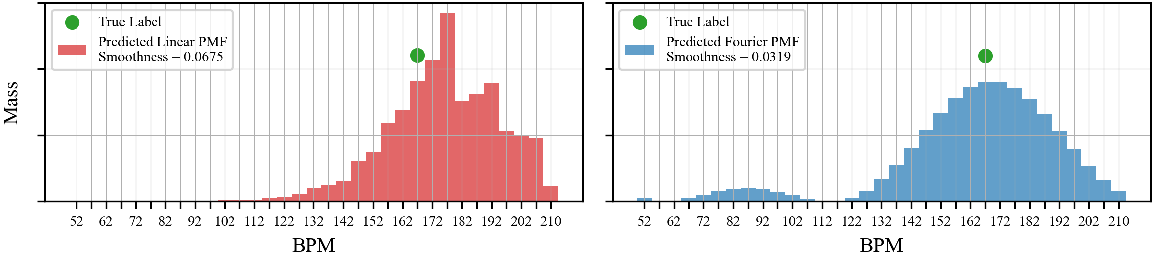
Figure 2: Comparison between the PMF learned by the linear head, and the Fourier head with 2 frequencies, for the toy BPM classification task, on a single audio example. We observe that the Fourier head learns a smoother categorical distribution over its predicted values, and is better centered around the ground truth label. We also note the small mini-sine wave artifacting on the left side of the Fourier model, which tends to occur when using few frequencies.

2.4 Fourier Head: Considerations for Using it During Training

We highlight the main design choices for a user when applying the Fourier head in practice.

Training objective: The Fourier head inputs a signal $x\in\mathbb{R}^{n}$ and extracts from that signal an intermediate representation of a probability distribution $p_{x}(z)$ defined over $z\in[-1,1]$. This probability distribution has a closed formula equal to a Fourier series. In our experiments, we optimize the parameters of the Fourier PDF by discretizing it over the latent space and training using cross entropy loss. However, we should note that the Fourier layer allows MLE training directly on continuous values, by evaluating the Fourier PDF directly on the ground truth value in the latent space. But for consistency of comparison, and to demonstrate how easy it is to swap the Fourier head with a linear layer, we use softmax cross-entropy loss as the objective.

Choice of hyperparameter $N$: The Fourier head has one crucial hyperparameter–namely, the number of frequencies. How should one choose this in practice? We offer Theorem 3.3 as guiding principle beyond simple trial and error. This result provides a scaling law which formalizes the smoothness-expressive power trade-off in choosing the number of frequencies. In general, using more frequencies leads to more expressive power, and generally better success metrics, but at the cost of a learning less smooth densities, as well as more model parameters.

Fourier regularization: A generic Fourier series such as Equation 2.1 has Fourier coefficients which decay quickly enough for the infinite series to converge absolutely. For example, for the class of Fourier series which have continuous second derivatives, the Fourier coefficients decay on the order of $1/k^{2}$. To impose this regularity assumption on the learned Fourier densities, we follow (De la Fuente et al., 2024) and add a regularization term to the loss to prevent higher order Fourier coefficients from growing too large during training. This helps ensure that the learned Fourier PDF doesn’t overfit to noise in the data. In the notation from Algorithm 1, this means adding a regularization term of $\gamma\cdot\frac{2\pi^{2}}{m}\sum_{k=1}^{m}k^{2}|c_{n}|^{2}$ to the loss function, where $\gamma$ is a hyperparameter. We find that in the low-frequency domain, using $\gamma=0$ can give better performance than $\gamma>0$; and in the high frequency domain, $\gamma=10^{-6}$ works well.

Binning strategy: The choice of how we bin the data can affect performance significantly. As we already discussed, we should only apply the Fourier head when nearby bins are “similar” in some sense. This means we should order our bins in a semantically meaningful ordering. Further, in the case where the bins represent quantized numerical values over a continuous latent space, it can be helpful to use a “mixed-precision” binning strategy. For instance, if we want to model all values from $[-15,15]$, but we find that most values lie in the range $[-1,10]$, then we should allocate a higher proportion of bins to the dense data interval. Specifically, if we would like to use $m$ total bins to quantize the data, then we control the allocation of bins using a hyperparameter $d\in[0,1)$, where $\lfloor d\cdot m\rfloor$ uniformly spaced bins are allocated to the sparse data interval while the remaining $m-\lfloor d\cdot m\rfloor$ bins are allocated to the dense range (estimated from training data). This is motivated and supported by the Fourier theory as well, since by increasing precision in the dense data range we are effectively de-localizing the quantized data distribution, which leads to a more localized Fourier spectrum. This lets us obtain a quicker decay of higher frequency content, which ensures that we can more effectively learn the same distribution with lower-frequency Fourier heads.

Weight initialization: The learned parameters for the Fourier head consist of the learned linear layer which extracts autocorrelation parameters. In PyTorch, the linear layers uses the He initialization (He et al., 2015) by default, which ensures that the linear layer outputs values close to zero in expectation. Similarly, it’s better for the learning dynamics for the Fourier densities to be initialized to uniform $p(z)\approx 1/2$. We accomplish this by dividing the weights and biases by a large number, such as $1000$, after He initialization; this guarantees that the linear layer outputs very small values, so that Fourier coefficients output from the autocorrelation step are very small as well.

3 Theory

3.1 “Smoothness”: A Metric for High Frequency Content

In this section we propose a smoothness metric which inputs a categorical distribution $y=(y_{1},\dots,y_{m})\in\mathbb{R}^{m}$, and assigns a numerical value depending on how smooth it is. The score will output $0$ if $y$ is the smoothest possible categorical distribution, and larger values if $y$ is less smooth. We will first specify what we mean by “smooth”:

Heuristic 3.1.

We say a function is smooth if it contains very little high-frequency information.

For example, the uniform categorical distribution contains no high-frequency information, so it is the smoothest possible function, and should get a smoothness score of $0$. In contrast, a categorical distribution containing samples from $\sin(100\pi x)$ contains lots of high frequency information, so it should get a smoothness score greater than $0$. We seek to define a metric which measures smoothness according to Heuristic 3.1.

We will first develop a smoothness metric in the general case of a function $f:[a,b]\to\mathbb{R}$, then specialize to case of the discrete categorical distribution that we consider in the paper. If we let $\alpha_{\sigma}\in\mathbb{R}$ be weights satisfying $\int_{0}^{\infty}\alpha_{\sigma}d\sigma=1$, and $D$ be some measure of discrepancy such as $L^{2}$, and let $g_{\sigma}(x)*f(x)$ denote the convolution of $f(x)$ with a Gaussian kernel of standard deviation $\sigma$, then it is reasonable to define the smoothness of $f$ to be the quantity

$$s(f):=\int_{0}^{\infty}\int_{a}^{b}\alpha_{\sigma}D[f(x),g_{\sigma}(x)*f(x)]dxd\sigma.$$ (3.1)

In this expression, the discrepancy $D[f(x),g_{\sigma}(x)*f(x)]$ measures how different $f(x)$ is from a Gaussian-smoothed version of itself. Because the Gaussian is a low-pass filter, we can interpret Equation 3.1 as saying, at a high level, that a function is “smooth” if it doesn’t change that much when you remove high frequency content from it.

In our experiments, we consider discrete categorical distributions, and wish to evaluate how smooth they are in a numerically tractable way. Accordingly, we define a specific case of this as follows.

Definition 3.2 (Smoothness metric for categorical distributions).

Suppose $y=(y_{1},\dots,y_{m})\in\mathbb{R}^{m}$ is a categorical distribution, so every $y_{k}\geq 0$ and $\sum_{k=1}^{m}y_{k}=1$. Denote by $g_{\sigma}\in\mathbb{R}^{2m-1}$ the discrete Gaussian kernel of standard deviation $\sigma$ and radius $m-1$. Define the weights $\alpha_{\sigma}=6/\pi^{2}\sigma^{2}$. Then we define the smoothness of $y$ to be the constant

$$s(y):=\sum_{\sigma=1}^{\infty}\alpha_{\sigma}\|y-g_{\sigma}*y\|_{2}.$$ (3.2)

We direct the curious reader to Appendix B, where we conduct additional experiments to justify this choice of smoothness metric for our experiments.

3.2 A Scaling Law for the Fourier Head, in Frequency-aspect

In this subsection, we share a theorem that analyzes the quality of the Fourier head as the quantity of frequencies changes. We refer to this as the Fourier head scaling law as it quantifies the trade-off between modeling capacity and smoothness as the number of frequencies increases. On one hand, it is a celebrated result from Fourier analysis that a Fourier series with a greater number of frequencies models a larger class of functions; but on the other hand, we show that increasing frequencies also incurs loss in smoothness. This is to be expected, as we designed our smoothness metric with the intention of identifying a distribution as less smooth if it contains more high-frequency information.

Theorem 3.3.

(Fourier head scaling law.) Consider a Fourier head with input dimension $n$, output dimension $m$, and $N$ frequencies. Suppose that $1\ll N<\frac{m}{2}$. Then the following are true:

1. (Increasing $N$ improves modeling power.) As $N$ increases, the Fourier head is capable of learning a larger class of densities.

2. (Increasing $N$ degrades smoothness.) Consider an input to the Fourier head $x\in\mathbb{R}^{n}$, and denote by $f_{x}:[-1,1]\to\mathbb{R}$ the optimal conditional distribution that we would like the Fourier head to approximate for this input. Suppose that there exists some $t\geq 2$ such that the Fourier coefficients of $f_{x}$ decay on the order of $1/k^{t}$. Denote by $f_{x,N}$ the truncation of $f_{x}$ to its first $N$ frequencies, denote by $\vec{b}\in\mathbb{R}^{m}$ the $m$ bin centerpoints in $[-1,1]$, and denote by $y^{(N)}=f_{x,N}(\vec{b})/(f_{x,N}(b_{0})+\cdots+f_{x,N}(b_{m-1}))\in\mathbb{R}^{m}$ the discretization of $f_{x,N}$ into $m$ bins. Then, there exist constants $C_{1},C_{2}>0$ such that

   $$s(y^{(N)})=C_{1}-\frac{C_{2}}{N^{2t-1}}+O(1/N^{2t}).$$ (3.3)

Note that the smoothness scaling law asymptotic in Equation 3.3 shows that as $N$ increases, so does $s(y^{(N)})$. Further, note that if the Fourier spectrum of the underlying distribution decays quicker (controlled by $t$) then the rate at which smoothness degrades is slower; this is because if what we are learning has little high frequency content, then increasing the frequencies shouldn’t affect the smoothness of the learned distribution very much. In part (2), our assumption that the Fourier coefficients decay at least quadratically is reasonable since if $f_{x}$ is at least twice continuously differentiable, we already know its Fourier coefficients corresponding to the $k$-th frequency are in $O(1/k^{2})$ (Stein & Shakarchi, 2003, Ch.2, Cor. 2.4). Our Fourier quadratic weight decay regularization helps toward ensuring that this condition is met in practice as well. We include a full proof of this result in Appendix A.

4 Toy Example: Learning A Continuous Conditional Distribution

We demonstrate the advantage of using the Fourier head to learn a probability distribution for a simple task: learning the conditional distribution of the third number in the sequence given the first two. Here we will use $q(z)$ to denote the quantization of $z$.

Dataset: We create 3 synthetic datasets, which we name Gaussian, GMM, and GMM-2. Each dataset consists of $5000$ quantized triples $\{(q(x),q(y),q(z))\}\subseteq\mathbb{[}-1,1]^{3}$. Crucially, $z$ is sampled from a distribution which is conditioned on $x$ and $y$, and we have an explicit closed formula for this distribution. By design, the Gaussian dataset is unimodal in $z$, whereas the more challenging GMM and GMM-2 datasets are not unimodal. Full details about the datasets can be found in Appendix C.

Task: Predict the conditional distribution of $q(z)$ given the quantized tuple $(q(x),q(y))$.

Model architecture: Our model is an MLP with ReLU activations and one hidden layer, which maps $\mathbb{R}^{2}\to\mathbb{R}^{64}\to\mathbb{R}^{32}\to\mathbb{R}^{50}$. The output of the model has dimension $50$ because we quantize the interval $[-1,1]$ into 50 bins. For the baseline, the classification head is a linear layer followed by a softmax; for the Fourier model, the classification head is the Fourier head. We sweep over frequencies $N=2,4,\dots,20$, and we consider regularization $\gamma\in\{0,10^{-6}\}$. We train all models using cross entropy loss.

Model evaluation: We use three metrics for evaluation. Let $\mathcal{P}(x,y)$ denote the fixed conditional distribution of $z$ given $(x,y)$. Our first metric is the average KL divergence $D_{\text{KL}}(q(\mathcal{P}_{2}(x,y))||M(q(x),q(y)))$, where $M(q(x),q(y))$ denotes the predicted categorical conditional distribution of $q(z)$, and $q(\mathcal{P}(x,y))$ is the quantized approximation of $\mathcal{P}(x,y)$, where $\mathcal{P}(x,y)$ is the fixed conditional distribution, obtained by evaluating the density function of $\mathcal{P}(x,y)$ at the bin centers, multiplying by the bin width, and finally scaling by the sum of the likelihoods. Our second metric is MSE. To compute this, we use the point of maximum likelihood under the learned categorical distribution as a prediction for $q(z)$ and compute the difference between the prediction and true value in the test set. And our third metric is smoothness.

	KL Divergence ($\downarrow$)		Smoothness ($\downarrow$)
Dataset	Linear	Fourier	Linear	Fourier
Gaussian	0.170 $\pm$ 0.052	0.116 $\pm$ 0.043	0.116 $\pm$ 0.049	0.057 $\pm$ 0.011
GMM	0.185 $\pm$ 0.037	0.091 $\pm$ 0.004	0.078 $\pm$ 0.041	0.034 $\pm$ 0.010
GMM-2	0.238 $\pm$ 0.032	0.146 $\pm$ 0.033	0.068 $\pm$ 0.022	0.038 $\pm$ 0.007

Table 1: We compare metrics between the linear head, and the Fourier head with $12$ frequencies and no regularization (i.e. $\gamma=0$), for every dataset in our toy example. We observe that the Fourier head outperforms the linear head across all metrics. Notably, using Fourier head improves the KL divergence (the primary success metric) on average by approximately 40%. We aggregate metrics over 4 different seeds and report the standard deviation.

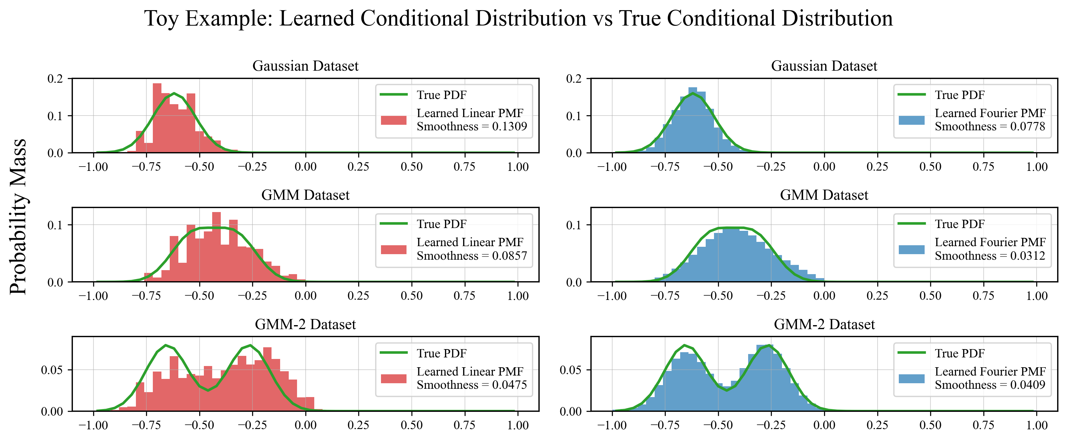
Figure 3: Comparison between the PMFs learned by the linear head, and the best performing Fourier head, for each of the datasets in the toy example. We observe that the Fourier head learns a smoother categorical distribution than the linear head over its predicted values. Furthermore, the Fourier head better fits the true conditional PDF; this is reflected in our KL divergence and smoothness metrics.

Results: The metrics for the best performing model on each dataset are reported in Table 1. Figure 3 presents sample visualizations of the learned conditional distributions alongside the true densities. And in Appendix C, we present the results of a study on the impact of number of frequencies and Fourier regularization. Notably, this study provides empirical evidence for the Fourier head scaling law in Theorem 3.3, as it demonstrates that for all datasets, as frequency increases, the smoothness degrades, and model performance improves until it reaches a saturation point. Crucially, we observe that the Fourier head flexibly learns all three distributions better than the linear baseline does. We note that the Fourier head outperforms the linear head on MSE as well; for details, see Appendix C.

5 Large-Scale Study: Offline Reinforcement Learning

The Decision Transformer (Chen et al., 2021) casts the problem of reinforcement learning as sequentially modeling rewards, states, and actions. Here, we study the performance of the Decision Transformer on the Seaquest game in the Atari (Bellemare et al., 2013) benchmark. The Seaquest game contains 18 actions, with two groups of eight actions that have a natural “closeness” metric defined on them: move left, up left, up, up right, right, down right, down, down left; as well as shooting in those eight directions. In their architecture, a decoder-only language model (Radford et al., 2018) encodes the context and then maps it through a linear layer, outputting a categorical distribution over the 18 possible actions. In our study, we replace that linear classification head with a Fourier head. Intuitively, this ought to give the model the prior that actions like “move left” and “move up left” are semantically similar, and therefore should have similar likelihoods. Our study confirms that the Fourier head outperforms the linear head in returns obtained by as much as $46\%$, in the reward conditioned setting considered in the paper, using identical training hyperparameters.

Dataset: We use the same dataset from the original Decision Transformer implementation (Chen et al., 2021). This dataset consists of 500k transitions experienced by an online deep Q-network agent (Mnih et al., 2015) during training on the Seaquest game.

Task: In the Seaquest game, the agent moves a submarine to avoid enemies, shoot at enemies, and rescue divers. The Seaquest game contains 18 actions: move left, up left, up, up right, right, down right, down, down left; as well as shooting in those eight directions; as well as no move, and a generic fire move. We consider this task in the Offline RL setting. The agent observes the past states, actions, and rewards, as well as the return-to-go, and attempts to predict the action that matches what an agent operating like the dataset would likely do.

Model architecture: (Chen et al., 2021) used the GPT-1 model (Radford et al., 2018) to autoregressively encode the context, which is then fed through a linear layer of dimension $18$, and the model ultimately optimizes the cross entropy loss between the action logits and the ground truth action from the dataset. We refer to this model as the linear baseline. To create our Fourier-$N$ version, we simply replace the linear head with a Fourier head with $N$ frequencies and Fourier regularization $\gamma=10^{-6}$. In our experiments we consider frequencies $N\in\{2,4,6,8,\dots,30,32\}$.

Model evaluation: We present mean reward totals for rollouts across $4$ seeds. In Table 2 we can see that normalized returns are as much as $46.2\%$ higher for sufficiently large frequencies. In Figure 4, we can see that, as we increase the quantity of frequencies, the returns increase and the learned PMFs become less smooth, in accordance with Theorem 3.3. Qualitatively, we can also see that in Figure 5 the PMFs learned by the Fourier head are smoother.

Decision Transformer Model	Normalized Return $(\uparrow)$	Smoothness $(\downarrow)$
Linear	2.53 $\pm$ 0.63	0.48 $\pm$ 0.14
Fourier-8	2.78 $\pm$ 0.47	0.22 $\pm$ 0.04
Fourier-14	3.70 $\pm$ 0.47	0.39 $\pm$ 0.11

Table 2: We present Decision Transformer results for the linear baseline, and for two representative Fourier head experiments. We observe that the Fourier head with 14 frequencies improves on the linear baseline by 46.2%. We report normalized return values (mean, and standard deviation) from (Chen et al., 2021), and we compute all other metrics ourselves. We compute the returns (mean and standard deviation) by averaging over four seeds, and we compute smoothness using all the evaluation rollouts from a single seed.

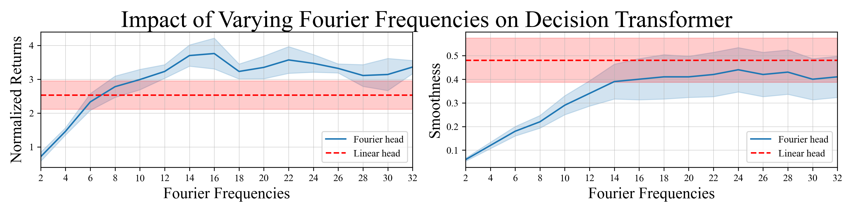
Figure 4: We present empirical results for how the quantity of Fourier frequencies impacts returns and smoothness for the imitation learning task. For normalized returns, higher is better; for smoothness, lower is better. We can see that the Fourier agent achieves higher normalized returns than the linear baseline agent when sufficiently many Fourier frequencies are used, while still learning smoother next-action distributions.

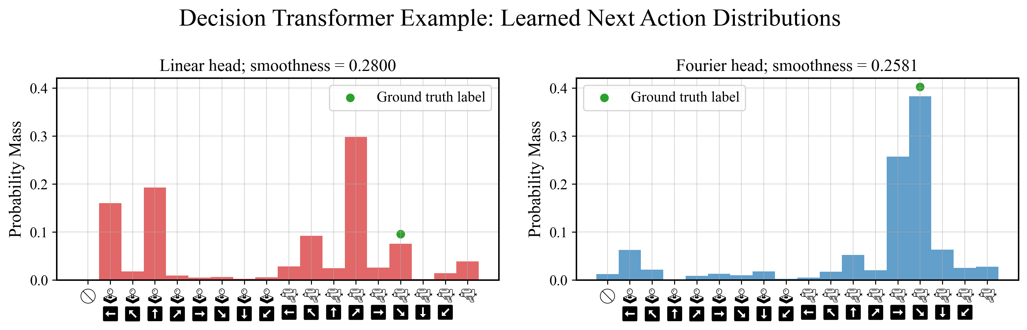
Figure 5: We present example next action distributions for a single step in the Decision Transformer test split. The Fourier agent with 8 frequencies produces a “clump” of actions that is semantically meaningful. Namely, this agent almost certainly wants to shoot in the down right or right direction, presumably because there is a submarine in that direction. In contrast, the linear agent’s next-action distribution doesn’t clearly depict a strategy, and incorrectly assigns higher likelihoods to incorrect actions. Because the Fourier head outputs a smoother PMF, it learns to concentrate more probability mass near the correct action.

Chronos Time Series Model	MASE $(\downarrow)$	WQL $(\downarrow)$	Smoothness $(\downarrow)$
Linear	0.883	0.750	0.1689 $\pm$ 0.1087
Fourier-64	0.875	0.798	0.0032 $\pm$ 0.0012
Fourier-128	0.872	0.767	0.0068 $\pm$ 0.0035
Fourier-256	0.859	0.755	0.0139 $\pm$ 0.0087
Fourier-550	0.852	0.749	0.0283 $\pm$ 0.0224
Fourier-550 (no regularization)	0.861	0.753	0.0286 $\pm$ 0.0219
Fourier-550 (uniform precision binning)	0.873	0.747	0.0395 $\pm$ 0.0252

Table 3: We present large-scale experiments on Chronos time series forecasting. Notably, every Fourier model outperforms the linear baseline on MASE and smoothness metrics. We can see that within the Fourier model class, decreasing the number of frequencies lets you trade off the continuity of the learned probability mass functions (smoothness) for the quality of the forecasts (MASE, WQL). In the bottom two rows, we present an ablation for our large-scale experiments on Chronos time series forecasting. The best overall performing Fourier-550 model uses Fourier regularization and mixed precision binning, which are both techniques informed by Fourier analysis. We observe that both of these interventions improve the MASE, but have minimal effect on the WQL. Note that the choice of binning strategy doesn’t affect the performance of the linear baseline.

6 Large-Scale Study: Probabilistic Time Series Forecasting

The Chronos time series foundation models (Ansari et al., 2024) “learn the language of time series”. They do this by approaching time series forecasting as language modeling, by tokenizing the quantized number line, learning token embeddings for each of those quantized values, and finally learning a categorical distribution to decide what the next value ought to be. This model is built on top of the encoder-decoder T5 model (Raffel et al., 2020). In particular, this model normalizes time series values to the range $[-15,15]$ and quantizes this interval into $4096$ tokens. As usual for language modeling, the final layer is a linear map which learns a categorical distribution over next tokens. In particular, we observe that token $i$ represents a number very close to tokens $i-1$ and $i+1$. However, we note that there is no inductive bias in the T5 architecture which pushes their likelihoods to be similar. This is not a hypothetical problem; in Figure 9 (Appendix), we can see that the linear next-token prediction PMFs fit to the noise, and appear very jagged.

The motivation for replacing the linear head with the Fourier head is to “smooth” out the distribution in the left side of Figure 9, to help the forecasting model better learn the signal, and ignore the noise. In this figure, we can see that the Fourier head accomplishes this successfully.

In this section, we study how the performance of the Chronos time series foundation model changes when we pre-train using the Fourier head, instead of the linear head. For all of the frequencies that we consider, the Fourier head outperforms the Chronos linear baseline on the MASE metric, while learning next token multinomials which are at least 8x smoother, with fewer parameters than the baseline.

Dataset: We use the same training dataset for large-scale pretraining that Ansari et al. (2024) used. We gather an evaluation benchmark of 20 time series datasets which were not seen during training. These 20 come from the zero-shot eval from (Ansari et al., 2024). The reader can check Appendix D for details on the training and evaluation datasets we used.

Model architecture: We use the Chronos model, which is built using the T5 architecture (Raffel et al., 2020). The original model has a linear classification head. For our study, we will replace this with a Fourier head with frequencies $N=64,128,256,550$. We use mixed precision binning; this is informed by an analysis of the Fourier spectrum of the next-token distribution, as described in Section 2.4. We also use Fourier quadratic weight decay regularization with $\gamma=10^{-6}$. For the task, the model learns to input time series context of length 512, and output a probabilistic forecast of length 64.

Model evaluation: We have two sets of metrics: model performance from (Ansari et al., 2024) (MASE measures the accuracy of median forecast, and WQL measures the quality of the probabilistic forecast), as well as our smoothness metric. Our Fourier metrics in Table 3 demonstrate that every Fourier model outperforms the linear baseline for MASE and smoothness. And for the largest Fourier model that we consider, Fourier outperforms linear on WQL as well. We also conduct an ablation study; the results in Table 3 show that mixed precision binning and regularization improve the MASE and smoothness for the Fourier head.

7 Related Work

LLMs outside of natural language domains: LLMs are often adapted to domains beyond natural language, as general purpose sequence models. For example, they have been used in protein synthesis (Madani et al., 2023), time series forecasting (Ansari et al., 2024; Das et al., 2024; Jin et al., 2024), music generation (Dhariwal et al., 2020; Agostinelli et al., 2023; Copet et al., 2023; Yuan et al., 2024), and as well as in decision making (Li et al., 2022; Chen et al., 2021).

We consider three categories to adapt LLMs to non-language domains: when the output of a language-trained LLM is used as a feature for some out-of-domain task; when a language-pretrained LLM is fine-tuned on a domain-specific task; and when an LLM architecture is trained on a domain-specific dataset from scratch. Our work directly considers the latter method of LLM adaptation, particularly in settings where the outputs approximate continuous values. We note that using LLMs to model numerical functions has seen success in continuing sequences (Mirchandani et al., 2023) but has been challenging for modeling samplers for probability distributions (Hopkins et al., 2023). In a related direction, Razeghi et al. (2022) found that model performance on numerical reasoning tasks is correlated with the frequency of specific numbers in its corpus. Further, some have re-framed continuous regression as a descretized classification problem to leverage LLMs in numerical modeling contexts (Song et al., 2024). While even frozen LLMs with no further training show interesting empirical results as regressors (Vacareanu et al., 2024), there is a conceptual mismatch between the downstream task and model construction because tokenized numerical values trained using cross-entropy loss does not explicitly enforce numerical relationships between the tokens.

Fourier series in neural networks: Many works leverage the Fourier transform as a data pre-processing step or a deterministic transformation within the network, or use Fourier analysis to motivate design choices. It is far less common to learn the Fourier series directly. De la Fuente et al. (2024) learned marginal univariate densities parameterized using a Fourier basis; our work extends their Fourier Basis Density model to multivariate settings with an autoregressive scheme. Our method learns conditional univariate densities using a Fourier basis, where the coefficients of the Fourier density model are input dependent. Sitzmann et al. (2020) proposed sinusoidal activation functions, which can be seen as learning the frequencies of a Fourier series; in contrast, we fix the frequencies to the canonoical choice $\{1,2,\dots,N\}$, and learn the amplitudes. This allows the Fourier head to directly benefit from approximation results from Fourier analysis.

8 Conclusion

We propose the Fourier head and demonstrate its positive impact on performance on several tasks. We prove a scaling law that characterizes the trade-off between the model’s expressivity and the smoothness of its output distribution. The Fourier head is a modular architecture that can be easily added to existing models that would benefit from the continuity inductive bias that the head imparts. The Fourier head extends the already extensive reach of LLMs into more diverse, numerical, and probabilistic domains. Future work includes exploring alternative training objectives that do not depend on discretizing probability density functions, and incorporating the Fourier head in general-purpose LLM training, where the head can be adaptively employed when needed.

Acknowledgments

We would like to thank Jona Balle, Alfredo De la Fuente, Calvin Luo, Singh Saluja, Matthew Schoenbauer, and Megan Wei for the useful discussions. This work is supported by the Samsung Advanced Institute of Technology, NASA, and a Richard B. Salomon Award for Chen Sun. Our research was conducted using computational resources at the Center for Computation and Visualization at Brown University.

Appendix A Proof of Fourier Head Scaling Law, Theorem 3.3

In this section we prove Theorem 3.3, the Fourier head scaling law. To do this, we must first discuss the Nyquist-Shannon Sampling Theorem. This result states that in order to avoid distortion of a signal (such as aliasing) the sampling rate must be at least twice the bandwidth of the signal. In the setting of the Fourier head, our sampling rate is $m/2$ because we have $m$ bins uniformly spaced in $(-1,1)$, and the bandwidth is $N/2$ because the frequency of $\sin(\pi Nx)$ is $N/2$. Thus the Nyquist Theorem requires us to have

$$m/2\geq 2\cdot(N/2)=N$$

in order for the higher order frequency content learned by our model to not be fallacious when we are learning from only $m$ bins. This justifies why we only theoretically study the case $1\ll N<m/2$ in the scaling law.

A.1 Definitions

Consider an input $x\in\mathbb{R}^{n}$ to the Fourier head, and denote by $f_{x}:[-1,1]\to\mathbb{R}$ the optimal conditional distribution that we would like the Fourier head to approximate for this input. We will assume that $f_{x}$ is periodic, since the Fourier head learns a $2$-periodic Fourier density. We denote by $f_{x,N}$ the truncation of the Fourier series of $f_{x}$ to its first $N$ frequencies. Note that $f_{x,N}$ also integrates to 1 over $[-1,1]$ since its first Fourier coefficient is the same as that of $f_{x}$. Further, $f_{x,N}$ is non-negative on $[-1,1]$ since its Fourier coefficients, being a subsequence of the coefficients of $f_{x}$, are non-negative definite; a periodic function with non-negative definite Fourier coefficients is non-negative by Herglotz’s Theorem (Brockwell & Davis, 1991, Corollary 4.3.2). For completeness, we will recall the convolution formulas, specialized to the cases we consider in our argument.

Definition A.1 (Discrete convolution).

Let $b_{j}:=-1+\frac{2j+1}{m},0\leq j<m$ be the center points of the $m$ bins in $(-1,1)$, and let us denote $\vec{b}:=(b_{0},\dots,b_{m-1})$. Denote by $G_{\sigma}(z):=\frac{e^{-z^{2}/2\sigma^{2}}}{\sqrt{2\pi}\sigma}$ the Gaussian PDF with standard deviation $\sigma$. Then the discrete Gaussian convolution filter of radius $m-1$ is

$$g_{\sigma}:=\frac{G_{\sigma}(\left[1-m,2-m,3-m,\dots,m-1\right])}{S(m,\sigma)}\in\mathbb{R}^{2m-1},$$ (A.1)

where the normalization constant is

$$S(m,\sigma):=\sum_{k=1-m}^{m-1}G_{\sigma}(k).$$ (A.2)

The discrete convolution of $g_{\sigma}\in\mathbb{R}^{2m-1}$ and $f_{x,N}(\vec{b})\in\mathbb{R}^{m}$ is the vector $(g_{\sigma}*f_{x,N})(\vec{b})\in\mathbb{R}^{m}$ whose $j$’th coordinate is given by

$$(g_{\sigma}*f_{x,N})(b_{j})=\frac{1}{S(m,\sigma)}\sum_{k=1-m}^{m-1}G_{\sigma}(k)\cdot f_{x,N}\left(b_{j-k}\right).$$ (A.3)

Definition A.2 (Continuous convolution).

The continuous Gaussian convolution filter $\tilde{g}_{\sigma}:\mathbb{[}-2,2]\to\mathbb{R}_{>0}$ is

$$\tilde{g}_{\sigma}(z)=\frac{G_{\frac{2\sigma}{m}}(z)}{S(m,\sigma)}=\frac{m}{2S(m,\sigma)}G_{\sigma}\left(\frac{mz}{2}\right).$$ (A.4)

This function $\tilde{g}_{\sigma}(z)$ is a normalized truncation of a Gaussian PDF with mean $0$ and standard deviation $2\sigma/m$. The continuous convolution of $\tilde{g}_{\sigma}:[-2,2]$ and the periodic function $f_{x,N}:[-1,1]\to\mathbb{R}$ is

$$\tilde{g}_{\sigma}*f_{x,N}(z):=\int_{-2}^{2}\tilde{g}_{\sigma}(u)f_{x,N}(z-u)\,du.$$ (A.5)

A.2 Overview of proof

In this subsection, we provide an overview of the proof of Theorem 3.3 by presenting the statements of the lemmata that we will need, and connecting each one to the overall argument. In the next subsection, we rigorously prove the scaling law by careful applications of these lemmata. And in the following subsection, we will rigorously prove each of the lemmata.

This first lemma allows us to replace the discrete Gaussian convolution in the definition with a continuous Gaussian convolution.

Lemma A.3.

(Discrete convolution is close to continuous convolution) If we define the constant $B_{1}(m,\sigma):=1+\frac{G_{\sigma}(m)}{S(m,\sigma)}$, then we have that

$$\|f_{x,N}(\vec{b})-g_{\sigma}*f_{x,N}(\vec{b})\|_{2} =\|B_{1}(m,\sigma)f_{x,N}(\vec{b})-\tilde{g}_{\sigma}*f_{x,N}(\vec{b})\|_{2}+\sqrt{m}O(1/N^{2t+1}).$$ (A.6)

Furthermore, $B_{1}(m,\sigma)$ satisfies the following bound, uniformly in $\sigma$,

$$B_{1}(m,\sigma)\leq 1+\frac{1}{2m-1}.$$ (A.7)

This next lemma, a standard result from analytic number theory allows us to upper bound the sums of the norms of the Fourier series coefficients. This is proved in various places, see e.g. (Tao, 2014, Equation 21).

Lemma A.4 (Asymptotic expansion of Riemann zeta function).

Consider the Riemann zeta function $\zeta(t):=\sum_{k=1}^{\infty}\frac{1}{k^{t}}$. If $t\geq 2$, then

$$\sum_{k=1}^{N}\frac{1}{k^{t}}=\zeta(t)-\frac{1}{t-1}\frac{1}{N^{t-1}}+O(1/N^{t}).$$ (A.8)

This next lemma allows us to extract the main asymptotic behavior in the scaling law.

Lemma A.5.

(Main term asymptotic) Denote by $a_{0}(x)$ the constant coefficient of $f_{x,N}$. Let us suppose that the Fourier coefficients of $f_{x,N}$ decay like $B_{3}(x)/k^{t}$, and define the constant

$$B_{2}(\sigma,m,x):=\sqrt{a_{0}(x)^{2}B_{1}(m,\sigma)^{2}+2B_{1}(m,\sigma)^{2}B_{3}(x)^{2}\zeta(2t)}.$$ (A.9)

Then we know that

$$\|B_{1}(m,\sigma)f_{x,N}(\vec{b})-\tilde{g}_{\sigma}*f_{x,N}(\vec{b})\|_{2} =\sqrt{m}\left(B_{2}(\sigma,m,x)-\frac{B_{1}(m,\sigma)^{2}B_{3}(x)^{2}}{2t-1}\cdot\frac{1}{N^{2t-1}}+O(1/N^{2t})\right).$$ (A.10)

Furthermore, $B_{2}(\sigma,m,x)$ is bounded from above and below as a function of $\sigma$ and $m$.

This final lemma allows us to relate the continuous case, where our analysis works out easier, to the discrete case, where our smoothness metric is actually defined.

Lemma A.6.

(The average value of the truncated Fourier PDF is $1/2$) If $N<m/2$, then

$$\sum_{j=0}^{m-1}f_{x,N}(b_{j})=\frac{m}{2}.$$ (A.11)

A.3 Proving Theorem 3.3 using the lemmata

We now prove the theorem that provides a scaling law for the Fourier head. This result quantifies the trade-off between modeling capacity and smoothness as the number of frequencies increases. In order to prove this, we must assume that $f_{x}$, the conditional distribution being learned by the Fourier head, is sufficiently smooth. For example, if $f_{x}$ is twice continuously differentiable, then the Fourier coefficients corresponding to the $k$-th frequency of $f_{x}$ are in $O(1/k^{2})$ (Stein & Shakarchi, 2003, Ch.2, Cor. 2.4). Thus, our assumption that the Fourier coefficients decay quadratically is reasonable, and our Fourier quadratic weight decay regularization helps ensure that this condition is met in practice as well. In our theorem, we generalize this hypothesis to the cases where the Fourier coefficients corresponding to the $k$-th frequency of $f_{x}$ are in $O(1/k^{t})$.

See 3.3

Proof of Claim 2 of Theorem 3.3.

We can estimate that

$$s(y^{(N)}) =\frac{1}{\sum_{j=0}^{m-1}f_{x,N}(b_{j})}\sum_{\sigma=1}^{\infty}\alpha_{\sigma}\|f_{x,N}(\vec{b})-g_{\sigma}*f_{x,N}(\vec{b})\|_{2}$$ (Definition 3.2) (A.12)

$$=\frac{1}{\sum_{j=0}^{m-1}f_{x,N}(b_{j})}\sum_{\sigma=1}^{\infty}\alpha_{\sigma}\Big{(}\|B_{1}(m,\sigma)f_{x,N}(\vec{b})-(\tilde{g}_{\sigma}*f_{x,N})(\vec{b})\|_{2}$$ (Lemma A.3) (A.13)

$$\qquad\qquad\qquad\qquad\qquad\qquad\qquad+\sqrt{m}O(1/N^{2t+1})\Big{)}$$

$$=\frac{\sqrt{m}}{\sum_{j=0}^{m-1}f_{x,N}(b_{j})}\sum_{\sigma=1}^{\infty}\alpha_{\sigma}\Big{(}B_{2}(\sigma,m,x)-\frac{B_{1}(m,\sigma)^{2}B_{3}(x)^{2}}{(2t-1)N^{2t-1}}$$ (Lemma A.5) (A.14)

$$\qquad\qquad\qquad\qquad\qquad\qquad\qquad+O(1/N^{2t})+O(1/N^{2t+1})\Big{)}$$

$$=\frac{2}{\sqrt{m}}\cdot\left(C_{3}-\frac{C_{4}}{N^{2t-1}}+O(1/N^{2t})\right).$$ (Lemmata A.5, A.6) (A.15)

In the last step we used the convergence of the respective series (which follows from boundedness of $B_{2}(\sigma,m,x)$ and $B_{1}(m,\sigma)$ in $\sigma$) and we assigned $C_{3}$ and $C_{4}$ to be those sums. This completes the proof. ∎

Proof of Claim 1 of Theorem 3.3.

The proof of this claim is more straightforward. For any function $f$ on $[-1,1]$ that is at least twice continuously differentiable, we know that the Fourier series of $f$ converges uniformly and absolutely to $f$ (Stein & Shakarchi, 2003, Ch. 2, Cor. 2.4). In other words, the function $f_{N}$ being learnt by the Fourier head converges uniformly and absolutely to $f$. ∎

A.4 Proving all of the Lemmata

In this subsection, we will restate and prove Lemmata A.3, A.5, and A.6.

See A.3

Proof of Lemma A.3.

Extending $f_{x,N}$ periodically to $[-2,2]$, we can compute that the continuous convolution $\tilde{g}_{\sigma}*f_{x,N}(z)$ is

$$(\tilde{g}_{\sigma}*f_{x,N})(z) =\int_{-2}^{2}\tilde{g}_{\sigma}(u)f_{x,N}(z-u)\,du$$ (A.16)

$$=\frac{m}{2S(m,\sigma)}\int_{-2}^{2}G_{\sigma}\left(\frac{mu}{2}\right)f_{x,N}(z-u)\,du$$ (A.17)

$$=\frac{1}{S(m,\sigma)}\int_{-m}^{m}G_{\sigma}(s)f_{x,N}\left(z-\frac{2s}{m}\right)\,ds,$$ (A.18)

where in the third step we applied the change of variables $s=\frac{mu}{2}$. We claim that this is precisely a continuous approximation of the discrete convolution in Definition 3.2. To see this, we will apply the Euler-Maclaurin formula. This formula says that the integral in Equation A.18 is a Riemann sum over rectangles of width $1$ evaluated at the right endpoints of each interval, minus an error term $E(m,\sigma)$, as follows:

$$(\tilde{g}_{\sigma}*f_{x,N})(b_{j})+E(m,\sigma) =\frac{1}{S(m,\sigma)}\sum_{k=1-m}^{m}G_{\sigma}(k)\cdot f_{x,N}\left(b_{j}-\frac{2k}{m}\right)$$ (A.19)

$$=\frac{1}{S(m,\sigma)}\sum_{k=1-m}^{m}G_{\sigma}(k)\cdot f_{x,N}\left(-1+\frac{2j+1}{m}-\frac{2k}{m}\right)$$ (A.20)

$$=\frac{1}{S(m,\sigma)}\sum_{k=1-m}^{m}G_{\sigma}(k)\cdot f_{x,N}\left(-1+\frac{2(j-k)+1}{m}\right)$$ (A.21)

$$=\frac{1}{S(m,\sigma)}\left(\sum_{k=1-m}^{m-1}G_{\sigma}(k)\cdot f_{x,N}\left(b_{j-k}\right)+G_{\sigma}(m)f_{x,N}(b_{j-m})\right)$$ (A.22)

$$=\frac{1}{S(m,\sigma)}\left(S(m,\sigma)\cdot(g_{\sigma}*f_{x,N})(b_{j})+G_{\sigma}(m)f_{x,N}(b_{j})\right)$$ (A.23)

$$=(g_{\sigma}*f_{x,N})(b_{j})+\frac{1}{S(m,\sigma)}G_{\sigma}(m)f_{x,N}(b_{j}),$$ (A.24)

where the error term is defined as

$$E(m,\sigma) :=\frac{1}{S(m,\sigma)}{\int_{-m}^{m}\frac{d\left(G_{\sigma}(s)f_{x,N}\left(z-\frac{2s}{m}\right)\right)}{ds}{P_{1}(s)}\,ds}$$ (A.25)

$$\qquad+\frac{1}{2S(m,\sigma)}\left(G_{\sigma}(m)f_{x,N}(z-2)-G_{\sigma}(-m)f_{x,N}(z+2)\right),$$ (A.26)

where $P_{1}(s):=s-\lfloor s\rfloor-1/2$ is the periodized Bernoulli polynomial. We will now estimate this error term. Note that since $G_{\sigma}$ is an even function and $f_{x,N}$ is periodic with period $2$, the difference in A.26 is $0$. Therefore, we can compute that

$$E(m,\sigma) =\frac{1}{S(m,\sigma)}\int_{-m}^{m}G_{\sigma}^{\prime}(s)P_{1}(s)f_{x,N}\left(z-\frac{2s}{m}\right)\,ds$$ (A.27)

$$\qquad-\frac{2}{mS(m,\sigma)}\int_{-m}^{m}G_{\sigma}(s)P_{1}(s)f^{\prime}_{x,N}\left(z-\frac{2s}{m}\right)\,ds.$$ (A.28)

Using the triangle inequality, we can bound $E(m,\sigma)$ in terms of convolutions with $\tilde{g}_{\sigma}$:

$$\left|E(m,\sigma)\right| \leq\frac{1}{S(m,\sigma)}\left|\int_{-m}^{m}G_{\sigma}^{\prime}(s)P_{1}(s)f_{x,N}\left(z-\frac{2s}{m}\right)\,ds\right|$$ (A.29)

$$\qquad+\frac{1}{S(m,\sigma)}\left|\int_{-m}^{m}G_{\sigma}(s)P_{1}(s)f^{\prime}_{x,N}\left(z-\frac{2s}{m}\right)\frac{-2}{m}\,ds\right|$$ (A.30)

$$\leq\frac{1}{S(m,\sigma)}\left(\frac{m}{2\sigma^{2}}\int_{-m}^{m}G_{\sigma}(s)f_{x,N}\left(z-\frac{2s}{m}\right)\,ds+\frac{1}{m}\int_{-m}^{m}G_{\sigma}(s)\left|f^{\prime}_{x,N}\left(z-\frac{2s}{m}\right)\right|ds\right)$$ (A.31)

$$=\frac{m}{2\sigma^{2}}(\tilde{g}_{\sigma}*f_{x,N})(z)+\frac{1}{m}(\tilde{g}_{\sigma}*\left|f^{\prime}_{x,N}\right|)(z),$$ (A.32)

where in Equation A.31 we used that $\left|P_{1}(s)\right|\leq 1/2$ and that $\left|G^{\prime}_{\sigma}(s)\right|=\left|s\right|G_{\sigma}(s)/\sigma^{2}\leq mG_{\sigma}(s)/\sigma^{2}$ for $s\in[-m,m]$.

Note that since $\tilde{g}_{\sigma}$ is a truncated Gaussian on $[-2,2]$, it is infinitely differentiable on the open set $(-2,2)$, however, it is not differentiable at the endpoints $-2$ and $2$ when treated as a 4-periodic function. This technical difficulty can be resolved using mollifiers: we can replace $\tilde{g}_{\sigma}$ with $\tilde{g}_{\sigma}*\varphi_{\epsilon}$, where $\{\varphi_{\epsilon}\}$ is a family of mollifiers indexed by $\epsilon>0$. The key properties of a mollifier are that $\tilde{g}_{\sigma}*\varphi_{\epsilon}$ is infinitely differentiable as a 4-periodic function for all $\epsilon>0$ and $\lim_{\epsilon\to 0}\tilde{g}_{\sigma}*\varphi_{\epsilon}=\tilde{g}_{\sigma}$ (Stein & Shakarchi, 2005, Ch. 3). We are ultimately interested in only bounds on absolute values of $\tilde{g}_{\sigma}$ convolved with various functions, and since absolute values are continuous and inequalities are preserved under taking limits, all our bounds are still true. In particular, this shows that the $k$’th Fourier coefficients of $\tilde{g}_{\sigma}$ decay faster than any polynomial. And on the other hand, by assumption we know that the Fourier coefficients of $f_{x,N}$ decay on the order of $1/k^{t}$; and we know that $|f_{x,N}^{\prime}|$ is continuous and $2\pi$ periodic, so its Fourier coefficients converge. So by the convolution theorem, we can deduce that the Fourier coefficients of $\tilde{g}*f_{x,N}$ and $\tilde{g}_{\sigma}*|f_{x,N}^{\prime}|$ decay faster than any polynomial. Summed over the $N$ frequencies, this shows that $|\tilde{g}_{\sigma}*f_{x,N}(x)|$ and $|\tilde{g}_{\sigma}*\left|f^{\prime}_{x,N}\right|(z)|$ decay faster than any polynomial as well. Since $m$ is fixed and $\sigma\geq 1$, this implies that

$$\left|E(m,\sigma)\right| =O(1/N^{2t+1}).$$ (A.33)

Using Definition A.1 and Equation A.19, we have that

$$g_{\sigma}*f_{x,N}(b_{j}) =\frac{1}{S(m,\sigma)}\sum_{k=1-m}^{m}G_{\sigma}(k)\cdot f_{x,N}\left(b_{j}-\frac{2k}{m}\right)-\frac{1}{S(m,\sigma)}G_{\sigma}(m)f_{x,N}(b_{j})$$ (A.34)

$$=(\tilde{g}_{\sigma}*f_{x,N})(b_{j})+E(m,\sigma)-\frac{1}{S(m,\sigma)}G_{\sigma}(m)f_{x,N}(b_{j}).$$ (A.35)

If we define $C_{1}(m,\sigma):=\frac{G_{\sigma}(m)}{S(m,\sigma)}$, then Equation A.35 combined with A.33 together imply that

$$\Big{|}g_{\sigma}*f_{x,N}(b_{j})-\tilde{g}_{\sigma}*f_{x,N}(b_{j})+C_{1}(\sigma,m)f_{x,N}(b_{j})\Big{|}=O(1/N^{2t+1}).$$ (A.36)

Finally, we can estimate that

$$\|f_{x,N}(\vec{b})-g_{\sigma}*f_{x,N}(\vec{b})\|_{2} =\|f_{x,N}(\vec{b})-\tilde{g}_{\sigma}*f_{x,N}(\vec{b})+C_{1}(\sigma,m)f_{x,N}(\vec{b})\|_{2}$$ (A.37)

$$\qquad+\|g_{\sigma}*f_{x,N}(\vec{b})-\tilde{g}_{\sigma}*f_{x,N}(\vec{b})+C_{1}(m,\sigma)f_{x,N}(\vec{b})\|$$ (A.38)

$$=\|f_{x,N}(\vec{b})-\tilde{g}_{\sigma}*f_{x,N}(\vec{b})+C_{1}(m,\sigma)f_{x,N}(\vec{b})\|_{2}+\sqrt{m}\|O(1/N^{2t+1})\|_{2}$$ (A.39)

$$=\|(1+C_{1}(m,\sigma))f_{x,N}(\vec{b})-\tilde{g}_{\sigma}*f_{x,N}(\vec{b})\|_{2}+\sqrt{m}O(1/N^{2t+1}).$$ (A.40)

This completes the first part of the proof. For the second part of the proof, since $S(m,\sigma)\geq(2m-1)G_{\sigma}(m-1)$, we can estimate that

$$B_{1}(m,\sigma)\leq 1+\frac{G_{\sigma}(m)}{(2m-1)G_{\sigma}(m-1)}\leq 1+\frac{1}{2m-1}e^{-(2m-1)/2\sigma^{2}}\leq 1+\frac{1}{2m-1}.$$ (A.41)

This completes the proof. ∎

See A.5

Proof of Lemma A.5.

We will first argue that $B_{2}(\sigma,m,x)$, as a function of $\sigma$ and $m$, is bounded from above and below. Indeed, from its definition, $B_{2}(\sigma,m,x)\geq\sqrt{a_{0}(x)^{2}B_{1}(m,\sigma)^{2}}\geq|a_{0}(x)|.$ But the Fourier PDF has integral $1$ over $[-1,1]$, so its constant term is $a_{0}(x)=1/2$. This implies that $B_{2}(\sigma,m,x)\geq 1/2$. To see $B_{2}(\sigma,m,x)$ is bounded from above, we simply recall that in Lemma A.3 we showed that $\left|B_{1}(m,\sigma)\right|\leq 2$, which implies that $|B_{2}(\sigma,m,x)|\leq\sqrt{4a_{0}(x)^{2}+8B_{3}(x)^{2}\zeta(2t)}$. This shows that $B_{2}(\sigma,m,x)$ is bounded above and below as a function of $m$ and $\sigma$, as claimed.

Now, let $(d_{0}(x),\dots,d_{m-1}(x))\in\mathbb{R}^{m}$ be the discrete Fourier transform of $(B_{1}(m,\sigma)f_{x,N}-\tilde{g}_{\sigma}*f_{x,N})(\vec{b})\in\mathbb{R}^{m}$. For notational simplicity, we will write $B_{1}=B_{1}(m,\sigma)$ as long as $\sigma$ is fixed. By Plancherel’s Theorem, we have

$$\sum_{j=0}^{m-1}\left|(B_{1}f_{x,N}-\tilde{g}_{\sigma}*f_{x,N})(b_{j})\right|^{2} =\frac{1}{m}\sum_{k=0}^{m-1}\left|d_{k}(x)\right|^{2}.$$ (A.42)

Let $h_{\sigma,j}$ be the Fourier coefficients of $\tilde{g}_{\sigma}$, treated as a periodic function with period $4$, and defined over $[-2,2]$:

$$\tilde{g}_{\sigma}(z)=\sum_{j=-\infty}^{\infty}h_{\sigma,j}e^{\pi ijz/2}.$$ (A.43)

Since $f_{x,N}$ is defined over $[-1,1]$ and is periodic with period $2$, we can likewise treat it as a function over $[-2,2]$ with period $4$, in which case we can rewrite its Fourier series as

$$f_{x,N}(z)=\sum_{j=-2N}^{2N}\tilde{a}_{j}(x)e^{\pi ijz/2},$$ (A.44)

where

$$\tilde{a}_{j}(x)=\begin{cases}a_{j/2}(x)&\text{ if }j\equiv 0\pmod{2}\\ 0&\text{ else.}\end{cases}$$ (A.45)

Then, by the Convolution Theorem, we have

$$(B_{1}f_{x,N}-\tilde{g}_{\sigma}*f_{x,N})(b_{l}) =\sum_{j=-2N}^{2N}\tilde{a}_{j}(x)(B_{1}-h_{\sigma,j})\cdot e^{\pi ijb_{l}/2}$$ (A.46)

$$=\sum_{k=-N}^{N}\tilde{a}_{2k}(x)(B_{1}-h_{\sigma,2k})\cdot e^{\pi ikb_{l}}$$ (A.47)

$$=\sum_{k=-N}^{N}{a}_{k}(x)(B_{1}-h_{\sigma,2k})\cdot e^{\pi ikb_{l}},$$ (A.48)

where in the second equality we used the fact that $\tilde{a}_{j}$ is 0 for odd $j$ and therefore re-indexed using $k=j/2$. Thus, using the definition of DFT along with Equation A.48, we get

$$d_{k}(x) =\sum_{l=0}^{m-1}(B_{1}f_{x,N}-\tilde{g}_{\sigma}*f_{x,N})(b_{l})\cdot e^{-2\pi ikl/m}$$ (A.49)

$$=\sum_{l=0}^{m-1}\sum_{j=-N}^{N}a_{j}(x)(B_{1}-h_{\sigma,2j})e^{\pi ijb_{l}}\cdot e^{-2\pi ikl/m}$$ (A.50)

$$=\sum_{j=-N}^{N}a_{j}(x)(B_{1}-h_{\sigma,2j})\sum_{l=0}^{m-1}e^{\pi ij(-1+\frac{2l+1}{m})}\cdot e^{-2\pi ikl/m}$$ (A.51)

$$=\sum_{j=-N}^{N}a_{j}(x)(B_{1}-h_{\sigma,2j})\cdot e^{\pi ij(-1+1/m)}\sum_{l=0}^{m-1}e^{2\pi i(j-k)l/m}.$$ (A.52)

First, we claim that at most a single summand (in $j$) is represented. Towards this, we note that

$$\sum_{l=0}^{m-1}e^{2\pi i(j-k)l/m}=\begin{cases}0&j\not\equiv k\pmod{m}\\ m&j\equiv k\pmod{m}.\end{cases}$$ (A.53)

Then, we note that since $0<N<m/2$, for each $0\leq k<m$, there is at most one $j\in\{-N,-N+1,\dots,N\}$, such that $j\equiv k\pmod{m}$. This shows that there is at most a single summand. We will now find the exact formula for each summand. We consider three cases.

• Case 1: $0\leq k\leq N$. In this case, $j=k$ satisfies $j\equiv k\pmod{m}$, so this index gives the exponential sum of $m$.

• Case 2: $N<k<m-N$. In this case, $k$ is too large to be an index in the sum, so we can’t choose $j=k$; the next smallest equivalent value is $j=k-m$, which satisfies $j\equiv k\pmod{m}$. But $N-m<j<-N$ in this case, so $k$ is too small to be an index in the sum; therefore, every exponential sum is zero in this range.

• Case 3: $m-N\leq k\leq m-1$. In this case, $j=k-m$ satisfies $j\equiv k\pmod{m}$. We have $-N\leq j\leq 1$, so this is a valid index in the sum.

This gives the following closed formula:

$$d_{k}(x) =\begin{cases}m\cdot a_{k}(x)(B_{1}-h_{\sigma,2k})e^{\pi ik(-1+1/m)}&0\leq k\leq N\\ 0&N<k<m-N\\ m\cdot a_{k-m}(B_{1}-h_{\sigma,2(k-m)})e^{\pi i(k-m)(-1+1/m)}&m-N\leq k\leq m-1.\end{cases}$$ (A.54)

Using this closed formula in A.42, we obtain

$$\sum_{j=0}^{m-1}\left|(B_{1}f_{x,N}-\tilde{g}_{\sigma}*f_{x,N})(b_{j})\right|^{2} =\frac{1}{m}\sum_{k=0}^{N}\left|m\cdot a_{k}(x)(B_{1}-h_{\sigma,2k})e^{\pi ik(-1+1/m)}\right|^{2}$$ (A.55)

$$\qquad+\frac{1}{m}\sum_{k=m-N}^{m-1}\left|m\cdot a_{k-m}(B_{1}-h_{\sigma,2(k-m)})e^{\pi i(k-m)(-1+1/m)}\right|^{2}$$ (A.56)

$$=m\sum_{k=0}^{N}\left|a_{k}(x)(B_{1}-h_{\sigma,2k})\right|^{2}+m\sum_{k=m-N}^{m-1}\left|a_{k-m}(B_{1}-h_{\sigma,2(k-m)})\right|^{2},$$ (A.57)

where in the last step we used that $\left|e^{\pi ik(1-1/m)}\right|=1=\left|e^{\pi i(k-m)(1-1/m)}\right|$ since they are both complex exponentials. Now, since $\tilde{g}_{\sigma}$ is a real and even function, we know that its Fourier coefficients $h_{\sigma,k}$ are real. Further, since $\tilde{g}_{\sigma}$ is infinitely differentiable, we also know that $h_{\sigma,k}=O(1/k^{t})$ (in fact they decay faster than $1/k^{p}$ for any $p\geq 1$). Thus, using that $\left|a_{k}(x)\right|$ decays like $B_{3}(x)/k^{t}$, we see

$$\left|a_{k}(x)(B_{1}-h_{\sigma,2k})\right|^{2} =\left|a_{k}(x)\right|^{2}(B_{1}^{2}-2h_{\sigma,2k}(x)+h_{\sigma,2k}^{2})$$ (A.58)

$$=\frac{B_{3}^{2}B_{1}^{2}}{k^{2t}}+O\left(\frac{1}{k^{2t}(2k)^{t}}\right)+O\left(\frac{1}{k^{2t}(2k)^{2t}}\right).$$ (A.59)

From A.59, it is clear that since we are interested in only the dominant asymptotic, we can safely ignore the higher order terms coming from the $h_{\sigma,k}$. As a result, we can estimate that

$$\sum_{j=0}^{m-1}\left|(B_{1}f_{x,N}-\tilde{g}_{\sigma}*f_{x,N})(b_{j})\right|^{2} \approx mB_{1}^{2}a_{0}(x)^{2}+m\sum_{k=1}^{N}\frac{B_{3}^{2}B_{1}^{2}}{k^{2t}}+m\sum_{k=m-N}^{m-1}\frac{B_{3}^{2}B_{1}^{2}}{(k-m)^{2t}}$$ (A.60)

$$=ma_{0}(x)^{2}B_{1}^{2}+m\sum_{k=1}^{N}\frac{B_{3}^{2}B_{1}^{2}}{k^{2t}}+m\sum_{k=-N}^{-1}\frac{B_{3}^{2}B_{1}^{2}}{k^{2t}}$$ (A.61)

$$=ma_{0}(x)^{2}B_{1}^{2}+m\sum_{k=1}^{N}\frac{B_{3}^{2}B_{1}^{2}}{k^{2t}}+m\sum_{k=1}^{N}\frac{B_{3}^{2}B_{1}^{2}}{k^{2t}}$$ (A.62)

$$=ma_{0}(x)^{2}B_{1}^{2}+2m\sum_{k=1}^{N}\frac{B_{3}^{2}B_{1}^{2}}{k^{2t}}.$$ (A.63)

Next, we note that our asymptotic in Lemma A.4, applied at $2t$, yields

$$\sum_{k=1}^{N}\frac{1}{k^{2t}} =\zeta(2t)-\frac{1}{2t-1}\frac{1}{N^{2t-1}}+O(1/N^{2t}).$$ (A.64)

Substituting this into A.63, we obtain

$$\sum_{j=0}^{m-1}\left|(B_{1}f_{x,N}-\tilde{g}_{\sigma}*f_{x,N})(b_{j})\right|^{2} =ma_{0}(x)^{2}B_{1}^{2}+2mB_{1}^{2}B_{3}^{2}\left(\zeta(2t)-\frac{1}{2t-1}\frac{1}{N^{2t-1}}+O(1/N^{2t})\right)$$ (A.65)

$$=m\left(B_{2}^{2}-\frac{2B_{1}^{2}B_{3}^{2}}{2t-1}\frac{1}{N^{2t-1}}+B_{1}^{2}B_{3}^{2}O(1/N^{2t})\right)$$ (A.66)

$$=m\left(B_{2}^{2}-\frac{2B_{1}^{2}B_{3}^{2}}{2t-1}\frac{1}{N^{2t-1}}+O(1/N^{2t})\right),$$ (A.67)

where we defined $B_{2}=B_{2}(\sigma,m,x):=\sqrt{a_{0}(x)^{2}B_{1}^{2}+2B_{1}^{2}B_{3}^{2}\zeta(2t)}$ as in the statement of the Lemma, and in the third line we applied Lemma A.3 to estimate that $B_{1}\leq 2$, and we used that $B_{3}=B_{3}(x)$ only depends on $x$. Then, using the Taylor expansion $(1+x)^{1/2}=1+\frac{x}{2}+O(x^{2})$ about $0$, we can estimate that

$$\left(\sum_{j=0}^{m-1}\left|(B_{1}f_{x,N}-\tilde{g}_{\sigma}*f_{x,N})(b_{j})\right|^{2}\right)^{1/2} =\left(mB_{2}^{2}-\frac{m2B_{1}^{2}B_{3}^{2}}{2t-1}\frac{1}{N^{2t-1}}+mO(1/N^{2t})\right)^{1/2}$$ (A.68)

$$=\sqrt{m}B_{2}\left(1-\frac{2B_{1}^{2}B_{3}^{2}}{(2t-1)B_{2}^{2}}\frac{1}{N^{2t-1}}+\frac{1}{B_{2}^{2}}O(1/N^{2t})\right)^{1/2}$$ (A.69)

$$=\sqrt{m}B_{2}\left(1-\frac{1}{2}\cdot\frac{2B_{1}^{2}B_{3}^{2}}{(2t-1)B_{2}^{2}}\frac{1}{N^{2t-1}}+O(1/N^{2t})\right)$$ (A.70)

$$=\sqrt{m}\left(B_{2}-\frac{B_{1}^{2}B_{3}^{2}}{2t-1}\cdot\frac{1}{N^{2t-1}}+O(1/N^{2t})\right).$$ (A.71)

To justify our application of the Taylor expansion, we note that $N\gg 1$, and $B_{2}=B_{2}(\sigma,m,x)$ is bounded below as a function of $\sigma$ and $m$. This completes the proof. ∎

See A.6

Proof of Lemma A.6.

Denote by $a_{k}$ the Fourier coefficients of $f_{x,N}$. We can compute that

$$\sum_{j=0}^{m-1}f_{x,N}(b_{j}) =\sum_{j=0}^{m-1}\sum_{k=-N}^{N}a_{k}e^{i\pi k\left(-1+\frac{2j+1}{m}\right)}$$ (A.72)

$$=\sum_{k=-N}^{N}a_{k}e^{-i\pi k}e^{\frac{i\pi k}{m}}\sum_{j=0}^{m-1}e^{\frac{2\pi ijk}{m}}.$$ (A.73)

Note that by hypothesis, $N<m/2$, which implies that $|k|<m$ for every outer sum index $k$. We consider two cases; if $k=0$, then the innermost summand is $e^{\frac{2\pi ijk}{m}}=1$; and if $k\neq 0$, then the innermost sum is a truncated geometric series with first term $1$, common ratio $e^{\frac{2\pi ik}{m}}$, and $m$ terms. In summary, the innermost summand is

$$\sum_{j=0}^{m-1}e^{\frac{2\pi ijk}{m}} =\begin{cases}m&k=0\\ 0&k\neq 0,\end{cases}$$ (A.74)

which implies that $\sum_{j=0}^{m-1}f_{x,N}(b_{j})=ma_{0}$. But $a_{0}=1/2$ because $f_{x,N}$ is a PDF implies it has average value $1/2$ over $[-1,1]$. This completes the proof. ∎

Appendix B Smoothness Metric

We will examine how the proposed smoothness metric Equation 3.1 behaves in a toy example setting to gain intuition for its behavior. Consider a square wave, which can be expressed as an infinite sum of odd integer harmonics that decay in amplitude proportional to their frequency:

$$f(x)=\frac{4}{\pi}\sum_{n=1,3,5,\ldots}^{\infty}\frac{1}{n}\sin\left(\frac{n\pi x}{L}\right).$$ (B.1)

Here, the wavelength is $2L$ (Weisstein, 2024).

We construct a truncated version of the square wave with a finite and fixed number of frequencies. The waveform will slowly approach its jagged, square shape as more sine waves are added. We frame these increasingly jagged waves as descritized multinomial densities to simulate the output of the Fourier head. To do this, we simply set the height to zero when the wave crest becomes negative and normalize the sum to $1$. The output of this transformation for a few representative waveforms is pictured in Figure 6.

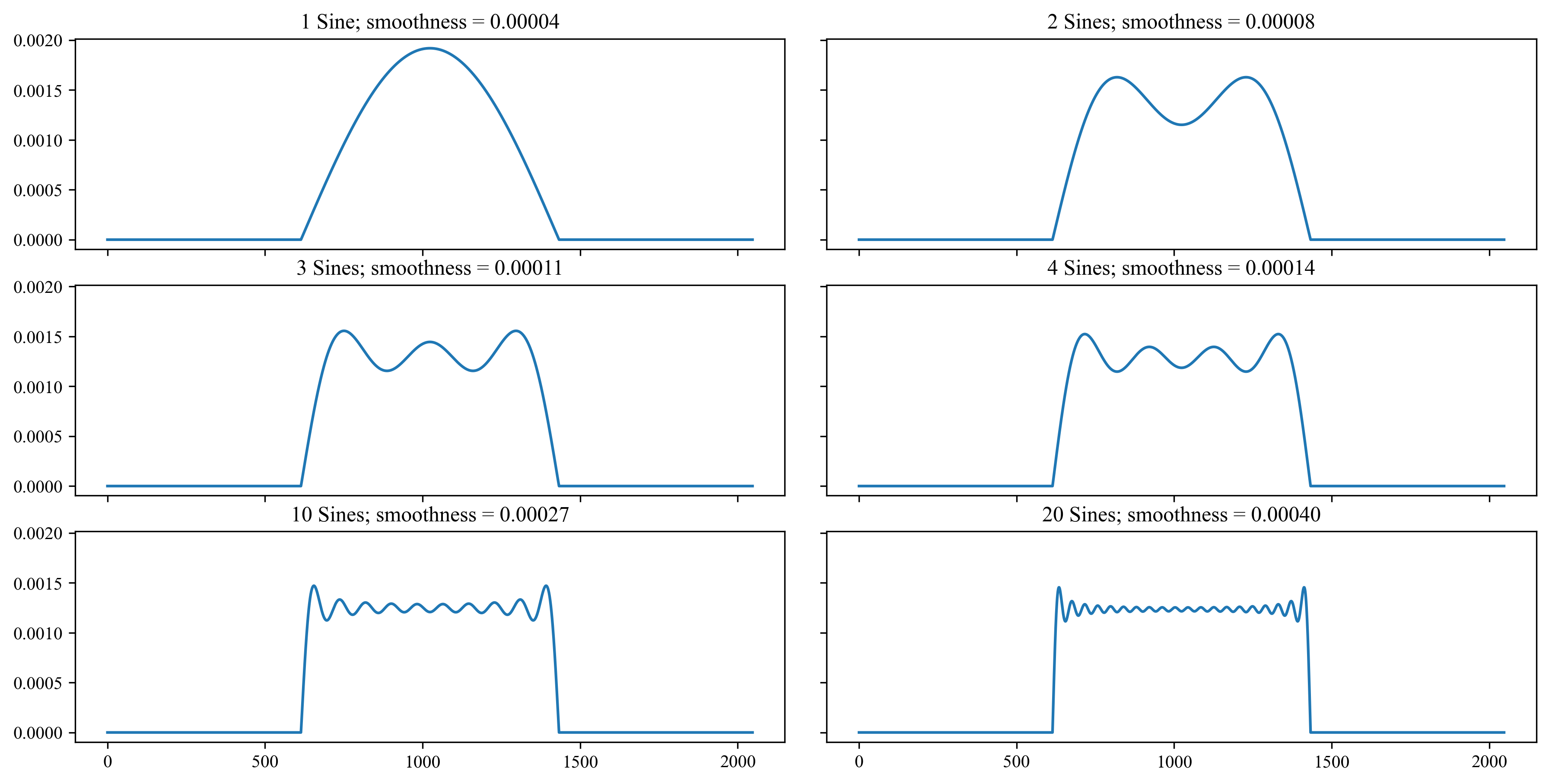
Figure 6: Truncated square waves framed as densities and their smoothness.

Intuitively, the truncated square wave with a single sine wave ought to be the smoothest. Thus our metric in this context should be smallest at that point, and increase monotonically as we add more sine waves. The plot in 7 demonstrates that this is indeed the case.

Choice of L2 Distance over L1 Distance: The proposed smoothness metric Equation 3.1 permits a general measure of discrepancy $D$, and we’ve chosen $D$ to be $L^{2}$ distance as indicated in 3.2. We empirically observe that $L^{2}$ distance better preserves monotonicity than the $L^{1}$ for higher frequency content, thus motivating this choice. With a sample rate of $2048$Hz, the $L^{1}$ distance exhibits some undesirable warping when our square-wave multinomial uses over 80 sine waves (see Figure 7). A Fourier head in a practical setting may possess several more than $80$ frequencies; accordingly, we favor the $L^{2}$ distance as our discrepancy measure.

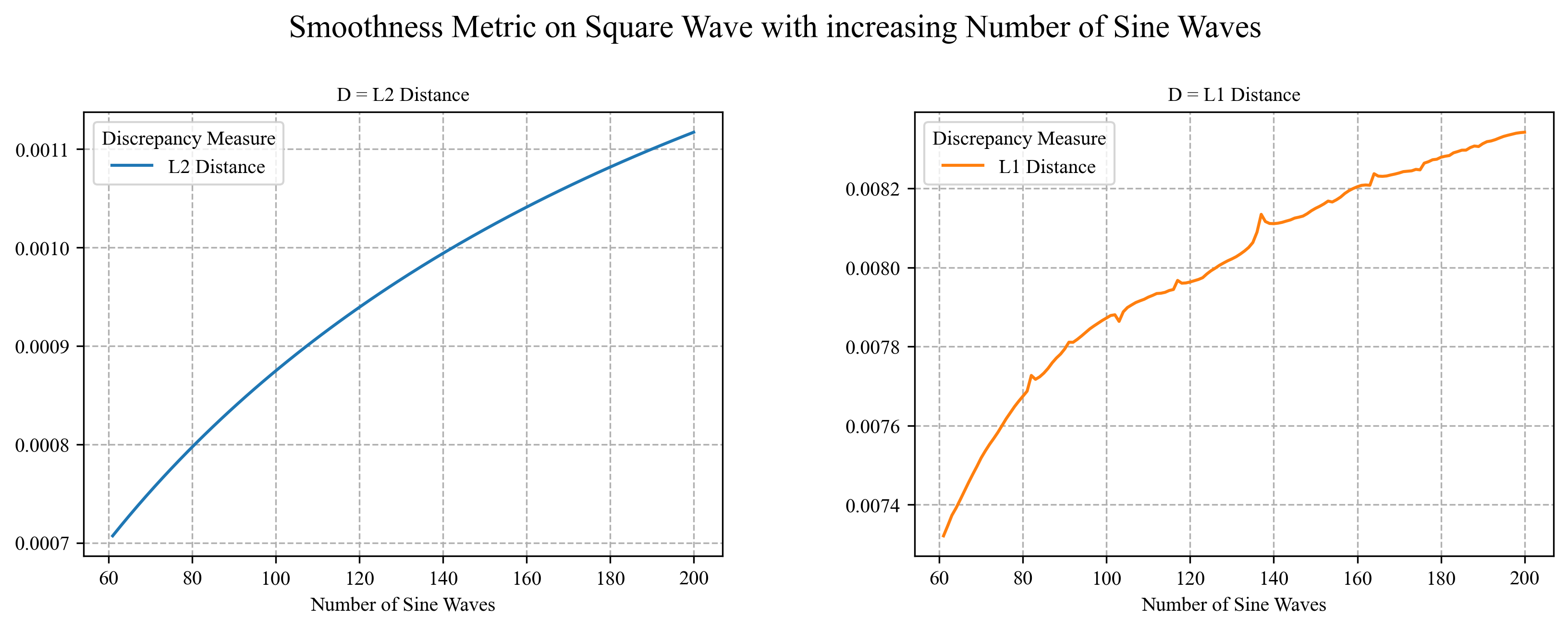
Figure 7: Values of the smoothness metric 3.2 on our square-wave-like multinomials as we increase the number of sine waves. We desire the value of this metric to be close to zero when there are few sine waves, and be monotonically increasing with each additional wave, indicating that adding more high frequency content results in a less smooth distribution. On the right, we can see that $L^{1}$ as a discrepancy measure leads to non-monotonicity, motivating our choice of $L^{2}$ distance in measuring our results.

Alternative Notions of Smoothness: In validating our choice of smoothness metric, we compare it to the spectral entropy (Inouye et al., 1991), which has a similar purpose in quantifying the “smoothness” of the frequency content of a signal. Spectral entropy is defined as the Shannon entropy of the power spectral density of a sampled signal $f$, which is defined as follows:

$$H(f;N)=\sum_{n\in N}p(n)\log_{2}\left(\frac{1}{p(n)}\right)=-\sum_{n\in N}\frac{S_{n}}{S_{total}}\log_{2}\left(\frac{S_{n}}{S_{total}}\right)$$ (B.2)

Here, $N$ is the number of Fourier frequencies and $S$ is the power of a frequency $n\in N$; $S_{n}$ is the power spectrum of the $n$th frequency, and $S_{total}$ is the power of the signal using all $N$ frequencies. For some frequency at index $n$, $S_{n}/S_{total}$ is called its relative power and $\sum_{n\in N}\frac{S_{n}}{S_{total}}=1$ enables us to consider each frequency’s power as a probability.

In the discrete case, the maximum entropy distribution is the uniform distribution. Thus, white noise will have the highest spectral entropy. This has the consequence that power spectral densities have more high frequency information will have lower entropy than that of white noise, provided that there is a relationship between amplitude and frequency. More concretely, blue noise, which is defined by the amplitude increasing proportionally to the frequency, will have lower spectral entropy than white noise. We sought a metric that always quantified ‘sharper’ signals like blue noise as less smooth. In Table  4, we frame sampled noises of different types as multinomial distributions to match our model setting by normalizing their amplitudes to be in $[0,1]$ and normalizing their sum to $1$. Our noise types are defined before normalization, in order of smoothest to sharpest:

• Brown: $S\propto\frac{1}{F^{2}}$

• Pink: $S\propto\frac{1}{F}$

• White: $S\sim\mathcal{N}(0,1)$

• Blue: $S\propto F$

where $S$ is the power density and $F$ is the frequency. To obtain samples of each type, we first generate white noise. We do this by sampling a Gaussian with mean $0$ and standard deviation $1$ to obtain amplitudes for $t$ samples. We then apply the Fourier transform, and multiply (or divide) the amplitudes of each component by their frequency, and apply the inverse Fourier transform to recover the waveform. Finally we adjust the range of amplitudes of the signal to be within $[0,1]$ and normalize the sum to $1$.

Discrepancy	Noise	Mean $\pm$ Std. Deviation	Diff	Delta	Desired Delta
L2	Brown	0.0003 $\pm$ 0.0001	n/a	n/a	n/a
L2	Pink	0.0017 $\pm$ 0.0002	0.0014	+	+
L2	White	0.0034 $\pm$ 0.0003	0.0016	+	+
L2	Blue	0.0038 $\pm$ 0.0003	0.0005	+	+
Spectral Entropy	Brown	0.4516 $\pm$ 0.0894	n/a	n/a	n/a
Spectral Entropy	Pink	0.3878 $\pm$ 0.0603	-0.0638	-	+
Spectral Entropy	White	0.4266 $\pm$ 0.0614	0.0388	+	+
Spectral Entropy	Blue	0.4191 $\pm$ 0.0583	-0.0076	-	+

Table 4: Smoothness measurements for four types of noise bootstrap aggregated over 1,000 trials. The color red emphasizes how the value of Spectral Entropy is undesirably not monotonic increasing for what we consider increasingly “sharp” noise types.

Appendix C Toy example details

Here we provide full details of the datasets used in our toy example of learning a known conditional distribution.

Dataset: We create a synthetic dataset $\mathcal{D}=\{(q(x),q(y),q(z))\}\subset\mathbb{R}^{3}$ as follows. Fix a probability distribution $\mathcal{P}_{1}=\mathcal{P}_{1}(x)$ that is parameterized by one variable and a second distribution $\mathcal{P}_{2}=\mathcal{P}_{2}(x,y)$ parameterized by two variables. Fix an interval $I\subset\mathbb{R}$. Sample $x$ uniformly from $I$, sample $y\sim\mathcal{P}_{1}(x)$, and finally sample $z\sim\mathcal{P}_{2}(x,y)$. We can repeat this sampling procedure $N$ times to obtain a set of $N$ triples for which we know the conditional distribution of $z$ given $x$ and $y$. Finally, we quantize this set to a fixed number of uniformly spaced bins in the range $[-1,1]$ to obtain the dataset $\mathcal{D}_{\mathcal{P}_{1},\mathcal{P}_{2}}$. We will denote the quantization of $z$ by $q(z)$. We quantize into 50 bins and our dataset has size 5000, with a 80-20 split between the train and test set. We describe three choices for the distributions we used to create our datasets. We fix $I=[-0.8,0.8]$ and $\sigma^{2}=0.01$ in all of them.

1. Gaussian dataset: $\mathcal{P}_{1}(x)=\mathcal{N}(x,\sigma^{2}),$ and $\mathcal{P}_{2}(x,y)=\mathcal{N}(y,\sigma^{2})$.

2. GMM dataset: $\mathcal{P}_{1}(x)=\mathcal{N}(x,\sigma^{2})$, and $\mathcal{P}_{2}(x,y)$ is a GMM centered at $\min\{x,y\}-0.1$ and $\max\{x,y\}+0.1$ with variance $\sigma^{2}$.

3. GMM-2 dataset: $\mathcal{P}_{1}=\text{Uniform}(I)$, and $\mathcal{P}_{2}(x,y)$ is a GMM centered at $x$ and $y$ with variance $\sigma^{2}$.

Additional results: In Figure 8, we present results from training over a range of frequencies, and for each frequency we ran experiments with and without Fourier regularization. In Table 6 we present results on the MSE metric, that show that the Fourier head outperforms the linear classification head.

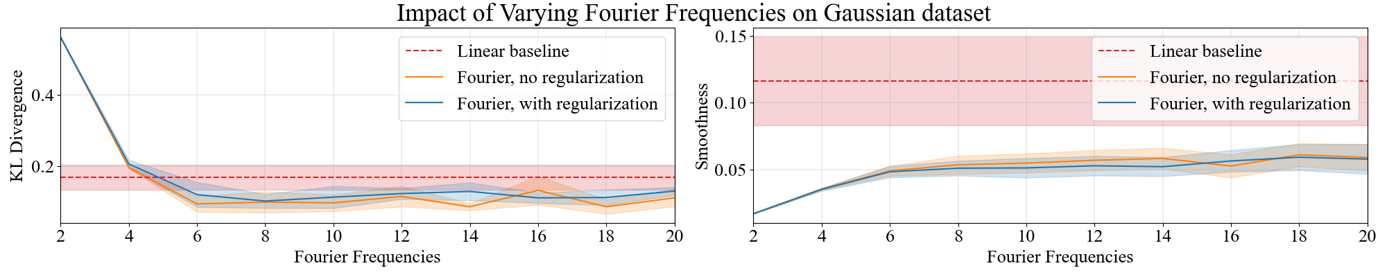
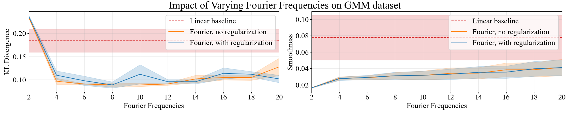
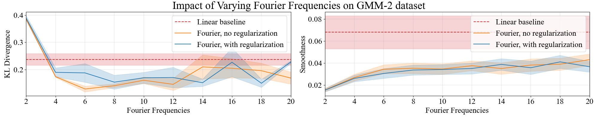
Figure 8: We study how the quantity of Fourier frequencies impacts KL divergence and smoothness for the toy example on each dataset. For both KL divergence and smoothness, lower is better. We observe that the Fourier models with and without regularization performed similarly to each other, and outperformed the linear baseline. We also note that the 50% error bars are larger for the linear baseline model; this indicates that the Fourier models (both with and without regularization) are in general more stable. This is in contrast to our large scale time series forecasting experiments, where we find that regularization helps; this is likely because those experiments use an order of magnitude more frequencies, and their conditional distributions are more complicated. Notice also how on each of the datasets, the smoothness degrades as frequency increases, in a fashion that follows the asymptotic from our Theorem 3.3(2).

	Linear	Fourier
Gaussian	0.013 $\pm$ 0.001	0.012 $\pm$ 0.001
GMM	0.041 $\pm$ 0.005	0.037 $\pm$ 0.002
GMM-2	0.224 $\pm$ 0.004	0.211 $\pm$ 0.016

Table 5: MSE ($\downarrow$)

Table 6: We compare the MSE between the linear head, and the Fourier head with $12$ frequencies and no regularization, on for every dataset in our toy example. We observe that the Fourier head outperforms the linear head across all metrics. We aggregate metrics over 4 different seeds and report the standard deviation.

Appendix D Additional Chronos experiment details

See Table 7 for the datasets we used to train and evaluate Chronos. And in Figure 9 we present a learned next-token PMF from a linear Chronos model, and a next-token PMF from a Chronos model which uses the linear head. The Fourier head is about 4x smoother. For all models in the paper, we use the “mini” version of the T5 model, as in (Ansari et al., 2024).

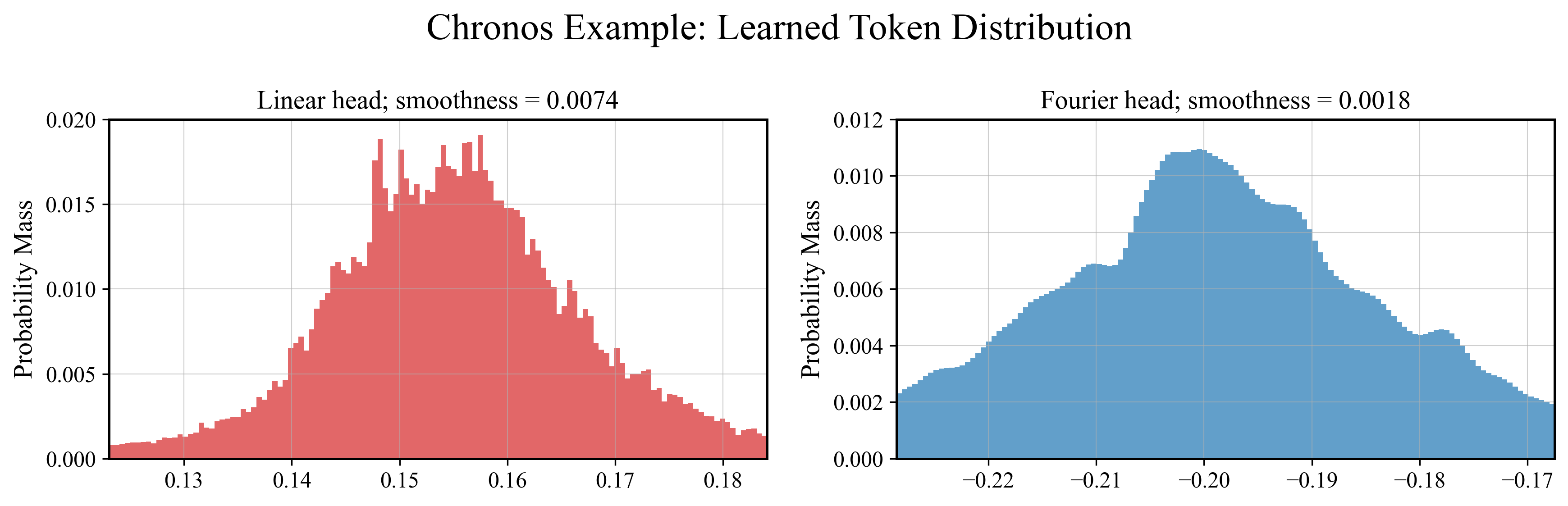
Figure 9: We present the next token value distribution for a single forecasted timestep on the Tourism Monthly dataset. We observe that the Fourier head’s learned conditional distribution is smoother, fitting signal more robustly, whereas the linear head overfits to the noise, and is therefore more jagged. We note that the $x$-axis represents the bins in the latent space $[-1,1]$; the $x$-axis values for the Fourier head are lower because the linear head uses uniform binning, and the Fourier head uses mixed precision binning.

Table 7: All datasets that are used for our time series forecasting experiments. We built our time series forecasting experiments on top of Chronos (Ansari et al., 2024), and this table is mostly copied from their paper. The datasets are partitioned according to how they are used for training and evaluation of models: pretraining-only data is only used for training; evaluation data is not used in training models, but only for evaluation (final $H$ observations). All of our evaluation datasets came from the zero-shot evaluation set from Chronos.

Dataset	Domain	Freq.	# Series	Series Length			Prediction
				min	avg	max	Length ($H$)
Pretraining
Brazilian Cities Temperature	nature	M	12	492	757	1320	-
Mexico City Bikes	transport	1H	494	780	78313	104449	-
Solar (5 Min.)	energy	5min	5166	105120	105120	105120	-
Solar (Hourly)	energy	1H	5166	8760	8760	8760	-
Spanish Energy and Weather	energy	1H	66	35064	35064	35064	-
Taxi (Hourly)	transport	1H	2428	734	739	744	-
USHCN	nature	1D	6090	5906	38653	59283	-
Weatherbench (Daily)	nature	1D	225280	14609	14609	14610	-
Weatherbench (Hourly)	nature	1H	225280	350633	350639	350640	-
Weatherbench (Weekly)	nature	1W	225280	2087	2087	2087	-
Wiki Daily (100k)	web	1D	100000	2741	2741	2741	-
Wind Farms (Daily)	energy	1D	337	71	354	366	-
Wind Farms (Hourly)	energy	1H	337	1715	8514	8784	-
Evaluation
Australian Electricity	energy	30min	5	230736	231052	232272	48
CIF 2016	banking	1M	72	28	98	120	12
Car Parts	retail	1M	2674	51	51	51	12
Hospital	healthcare	1M	767	84	84	84	12
M1 (Monthly)	various	1M	617	48	90	150	18
M1 (Quarterly)	various	3M	203	18	48	114	8
M1 (Yearly)	various	1Y	181	15	24	58	6
M3 (Monthly)	various	1M	1428	66	117	144	18
M3 (Quarterly)	various	3M	756	24	48	72	8
M3 (Yearly)	various	1Y	645	20	28	47	6
M4 (Quarterly)	various	3M	24000	24	100	874	8
M4 (Yearly)	various	1Y	23000	19	37	841	6
M5	retail	1D	30490	124	1562	1969	28
NN5 (Daily)	finance	1D	111	791	791	791	56
NN5 (Weekly)	finance	1W	111	113	113	113	8
Tourism (Monthly)	various	1M	366	91	298	333	24
Tourism (Quarterly)	various	1Q	427	30	99	130	8
Tourism (Yearly)	various	1Y	518	11	24	47	4
Traffic	transport	1H	862	17544	17544	17544	24
Weather	nature	1D	3010	1332	14296	65981	30

References

- Agostinelli et al. (2023) Andrea Agostinelli, Timo I Denk, Zalán Borsos, Jesse Engel, Mauro Verzetti, Antoine Caillon, Qingqing Huang, Aren Jansen, Adam Roberts, Marco Tagliasacchi, et al. Musiclm: Generating music from text. arXiv preprint arXiv:2301.11325, 2023.
- Ansari et al. (2024) Abdul Fatir Ansari, Lorenzo Stella, Caner Turkmen, Xiyuan Zhang, Pedro Mercado, Huibin Shen, Oleksandr Shchur, Syama Sundar Rangapuram, Sebastian Pineda Arango, Shubham Kapoor, et al. Chronos: Learning the language of time series. arXiv preprint arXiv:2403.07815, 2024.
- Bellemare et al. (2013) Marc G Bellemare, Yavar Naddaf, Joel Veness, and Michael Bowling. The arcade learning environment: An evaluation platform for general agents. Journal of Artificial Intelligence Research, 47:253–279, 2013.
- Brockwell & Davis (1991) Peter J Brockwell and Richard A Davis. Time series: theory and methods. Springer science & business media, 1991.
- Chen et al. (2021) Lili Chen, Kevin Lu, Aravind Rajeswaran, Kimin Lee, Aditya Grover, Michael Laskin, Pieter Abbeel, Aravind Srinivas, and Igor Mordatch. Decision transformer: Reinforcement learning via sequence modeling. arXiv preprint arXiv:2106.01345, 2021.
- Copet et al. (2023) Jade Copet, Felix Kreuk, Itai Gat, Tal Remez, David Kant, Gabriel Synnaeve, Yossi Adi, and Alexandre Défossez. Simple and controllable music generation. In Thirty-seventh Conference on Neural Information Processing Systems, 2023.
- Das et al. (2024) Abhimanyu Das, Weihao Kong, Rajat Sen, and Yichen Zhou. A decoder-only foundation model for time-series forecasting. In International Conference on Machine Learning, 2024.
- De la Fuente et al. (2024) Alfredo De la Fuente, Saurabh Singh, and Johannes Ballé. Fourier basis density model. arXiv preprint arXiv:2402.15345, 2024.
- Dhariwal et al. (2020) Prafulla Dhariwal, Heewoo Jun, Christine Payne, Jong Wook Kim, Alec Radford, and Ilya Sutskever. Jukebox: A generative model for music. arXiv preprint arXiv:2005.00341, 2020.
- Gemmeke et al. (2017) Jort F. Gemmeke, Daniel P. W. Ellis, Dylan Freedman, Aren Jansen, Wade Lawrence, R. Channing Moore, Manoj Plakal, and Marvin Ritter. Audio set: An ontology and human-labeled dataset for audio events. In Proc. IEEE ICASSP 2017, New Orleans, LA, 2017.
- Gong et al. (2021) Yuan Gong, Yu-An Chung, and James Glass. Psla: Improving audio tagging with pretraining, sampling, labeling, and aggregation. IEEE/ACM Transactions on Audio, Speech, and Language Processing, 2021. doi: 10.1109/TASLP.2021.3120633.
- He et al. (2015) Kaiming He, Xiangyu Zhang, Shaoqing Ren, and Jian Sun. Delving deep into rectifiers: Surpassing human-level performance on imagenet classification. In Proceedings of the IEEE international conference on computer vision, pp. 1026–1034, 2015.
- Hopkins et al. (2023) Aspen K Hopkins, Alex Renda, and Michael Carbin. Can llms generate random numbers? evaluating llm sampling in controlled domains. In ICML 2023 Workshop: Sampling and Optimization in Discrete Space, 2023.
- Inouye et al. (1991) Tsuyoshi Inouye, Kazuhiro Shinosaki, H. Sakamoto, Seigo Toi, Satoshi Ukai, Akinori Iyama, Y Katsuda, and Makiko Hirano. Quantification of eeg irregularity by use of the entropy of the power spectrum. Electroencephalography and Clinical Neurophysiology, 79(3):204–210, 1991. ISSN 0013-4694. doi: https://doi.org/10.1016/0013-4694(91)90138-T. URL https://www.sciencedirect.com/science/article/pii/001346949190138T.
- Jin et al. (2024) Ming Jin, Shiyu Wang, Lintao Ma, Zhixuan Chu, James Y Zhang, Xiaoming Shi, Pin-Yu Chen, Yuxuan Liang, Yuan-Fang Li, Shirui Pan, and Qingsong Wen. Time-LLM: Time series forecasting by reprogramming large language models. In International Conference on Learning Representations (ICLR), 2024.
- Li et al. (2022) Shuang Li, Xavier Puig, Chris Paxton, Yilun Du, Clinton Wang, Linxi Fan, Tao Chen, De-An Huang, Ekin Akyürek, Anima Anandkumar, et al. Pre-trained language models for interactive decision-making. Advances in Neural Information Processing Systems, 35:31199–31212, 2022.
- Liu et al. (2023) Yixin Liu, Avi Singh, C Daniel Freeman, John D Co-Reyes, and Peter J Liu. Improving large language model fine-tuning for solving math problems. arXiv preprint arXiv:2310.10047, 2023.
- Madani et al. (2023) Madani, Krause, and et al. Greene. Large language models generate functional protein sequences across diverse families. Nature Biotechnology, 41:1099–1106, 2023. doi: 10.1038/s41587-022-01618-2.
- Mirchandani et al. (2023) Suvir Mirchandani, Fei Xia, Pete Florence, Brian Ichter, Danny Driess, Montserrat Gonzalez Arenas, Kanishka Rao, Dorsa Sadigh, and Andy Zeng. Large language models as general pattern machines. In Proceedings of the 7th Conference on Robot Learning (CoRL), 2023.
- Mnih et al. (2015) Volodymyr Mnih, Koray Kavukcuoglu, David Silver, Andrei A Rusu, Joel Veness, Marc G Bellemare, Alex Graves, Martin Riedmiller, Andreas K Fidjeland, Georg Ostrovski, et al. Human-level control through deep reinforcement learning. nature, 518(7540):529–533, 2015.
- Radford et al. (2018) Alec Radford, Karthik Narasimhan, Tim Salimans, and Ilya Sutskever. Improving language understanding by generative pre-training. OpenAI website, 2018.
- Raffel et al. (2020) Colin Raffel, Noam Shazeer, Adam Roberts, Katherine Lee, Sharan Narang, Michael Matena, Yanqi Zhou, Wei Li, and Peter J Liu. Exploring the limits of transfer learning with a unified text-to-text transformer. Journal of machine learning research, 21(140):1–67, 2020.
- Razeghi et al. (2022) Yasaman Razeghi, Robert L Logan IV, Matt Gardner, and Sameer Singh. Impact of pretraining term frequencies on few-shot numerical reasoning. In Yoav Goldberg, Zornitsa Kozareva, and Yue Zhang (eds.), Findings of the Association for Computational Linguistics: EMNLP 2022, pp. 840–854, Abu Dhabi, United Arab Emirates, December 2022. Association for Computational Linguistics. doi: 10.18653/v1/2022.findings-emnlp.59.
- Sitzmann et al. (2020) Vincent Sitzmann, Julien Martel, Alexander Bergman, David Lindell, and Gordon Wetzstein. Implicit neural representations with periodic activation functions. Advances in neural information processing systems, 33:7462–7473, 2020.
- Song et al. (2024) Xingyou Song, Oscar Li, Chansoo Lee, Bangding Yang, Daiyi Peng, Sagi Perel, and Yutian Chen. Omnipred: Language models as universal regressors. CoRR, abs/2402.14547, 2024. doi: 10.48550/ARXIV.2402.14547. URL https://doi.org/10.48550/arXiv.2402.14547.
- Spivey (2008) Michael Spivey. The continuity of mind. Oxford University Press, 2008.
- Stein & Shakarchi (2003) Elias M Stein and Rami Shakarchi. Fourier analysis: an introduction, volume 1. Princeton University Press, 2003.
- Stein & Shakarchi (2005) Elias M Stein and Rami Shakarchi. Real Analysis: Measure Theory, Integration, and Hilbert Spaces, volume 3. Princeton University Press, 2005.
- Tao (2014) Terry Tao, Dec 2014. URL https://terrytao.wordpress.com/2014/12/09/254a-notes-2-complex-analytic-multiplicative-number-theory/#nxx.
- Vacareanu et al. (2024) Robert Vacareanu, Vlad Andrei Negru, Vasile Suciu, and Mihai Surdeanu. From words to numbers: Your large language model is secretly a capable regressor when given in-context examples. In First Conference on Language Modeling, 2024. URL https://openreview.net/forum?id=LzpaUxcNFK.
- Wei et al. (2024) Megan Wei, Michael Freeman, Chris Donahue, and Chen Sun. Do music generation models encode music theory? In International Society for Music Information Retrieval, 2024.
- Weisstein (2024) Eric W. Weisstein. Square wave. From MathWorld–A Wolfram Web Resource, 2024. URL https://mathworld.wolfram.com/SquareWave.html. Accessed: September 16, 2024.
- Yuan et al. (2024) Ruibin Yuan, Hanfeng Lin, Yi Wang, Zeyue Tian, Shangda Wu, Tianhao Shen, Ge Zhang, Yuhang Wu, Cong Liu, Ziya Zhou, Ziyang Ma, Liumeng Xue, Ziyu Wang, Qin Liu, Tianyu Zheng, Yizhi Li, Yinghao Ma, Yiming Liang, Xiaowei Chi, Ruibo Liu, Zili Wang, Pengfei Li, Jingcheng Wu, Chenghua Lin, Qifeng Liu, Tao Jiang, Wenhao Huang, Wenhu Chen, Emmanouil Benetos, Jie Fu, Gus Xia, Roger Dannenberg, Wei Xue, Shiyin Kang, and Yike Guo. Chatmusician: Understanding and generating music intrinsically with llm. arXiv preprint arXiv:2307.07443, 2024.