LipKernel: Lipschitz-Bounded Convolutional
Neural Networks via Dissipative Layers

Abstract

We propose a novel layer-wise parameterization for convolutional neural networks (CNNs) that includes built-in robustness guarantees by enforcing a prescribed Lipschitz bound. Each layer in our parameterization is designed to satisfy a linear matrix inequality (LMI), which in turn implies dissipativity with respect to a specific supply rate. Collectively, these layer-wise LMIs ensure Lipschitz boundedness for the input-output mapping of the neural network, yielding a more expressive parameterization than through spectral bounds or orthogonal layers. Our new method LipKernel directly parameterizes dissipative convolution kernels using a 2-D Roesser-type state space model. This means that the convolutional layers are given in standard form after training and can be evaluated without computational overhead. In numerical experiments, we show that the run-time using our method is orders of magnitude faster than state-of-the-art Lipschitz-bounded networks that parameterize convolutions in the Fourier domain, making our approach particularly attractive for improving robustness of learning-based real-time perception or control in robotics, autonomous vehicles, or automation systems. We focus on CNNs, and in contrast to previous works, our approach accommodates a wide variety of layers typically used in CNNs, including 1-D and 2-D convolutional layers, maximum and average pooling layers, as well as strided and dilated convolutions and zero padding. However, our approach naturally extends beyond CNNs as we can incorporate any layer that is incrementally dissipative.

I Introduction

Deep learning architectures such as deep neural networks (NNs), convolutional neural networks (CNNs) and recurrent neural networks have ushered in a paradigm shift across numerous domains within engineering and computer science [1]. Some prominent applications of such NNs include image and video processing tasks, natural language processing tasks, nonlinear system identification, and learning-based control [2, 3]. In these applications, NNs have been found to exceed other methods in terms of flexibility, accuracy, and scalability. However, as black box models NNs in general lack robustness guarantees, limiting their utility for safety-critical applications.

In particular, it has been shown that NNs are highly sensitive to small “adversarial” input perturbations [4]. This sensitivity can be quantified by the Lipschitz constant of an NN, and numerous approaches have been proposed for its estimation [5, 6, 7, 8]. While calculating the Lipschitz constant is an NP-hard problem [5, 9], computationally cheap but loose upper bounds are obtained as the product of the spectral norms of the matrices [4], and much tighter bounds can be determined using semidefinite programming (SDP) methods derived from robust control [7, 10, 8, 11, 12].

While analysis of a given NN is of interest, it naturally raises the question of synthesis of NNs with built-in Lipschitz bounds, which is the subject of the present work. Motivated by the composition property of Lipschitz bounds, most approaches assume 1-Lipschitz activation functions [13, 14] and attempt to constrain the Lipschitz constant (i.e., spectral bound) of matrices and convolution operators appearing in the network, however this can be conservative.

To impose more sophisticated linear matrix inequality (LMI) based Lipschitz bounds, [15, 16, 17] include constraints or regularization terms into the training problem. However, the resulting constrained optimization problem tends to have a high computational overhead, e.g., due to costly projections or barrier calculations [15, 16]. Alternatively, [18, 19, 20, 21] construct so-called direct parameterizations that map free variables to the network parameters in such a way that LMIs are satisfied by design, which in turn ensures Lipschitz boundedness for equilibrium networks [18], recurrent equilibrium networks [19], deep neural networks [20], and 1-D convolutional neural networks [21], respectively. The major advantage of direct parameterization is that it poses the training of robust NNs as an unconstrained optimization problem, which can be tackled with existing gradient-based solvers. In this work, we develop a new direct parameterization for Lipschitz-bounded CNNs.

Lipschitz-bounded convolutions can be parameterized in the Fourier domain, as in the Orthogonal and Sandwich layers in [22, 20], however this adds computational overhead of performing fast Fourier transforms (FFT) and their inverses, or alternatively full-image size kernels leading to longer computation times for inference. In contrast, in this paper we use a Roesser-type 2-D systems representation [23] for convolutions [24, 25]. This in turn allows us to directly parameterize the kernel entries of the convolutional layers, hence we denote our method as LipKernel. This direct kernel parameterization has the advantage that at inference time we can evaluate convolutional layers of CNNs in standard form, which can be advantageous for system verification and validation processes. It also results in significantly reduced compute requirements for inference compared to Fourier representations, making our approach especially suitable for real-time control systems, e.g. in robotics, autonomous vehicles, or automation. Furthermore, LipKernel offers additional flexibility in the architecture choice, enabling pooling layers and any kind of zero-padding to be easily incorporated.

Our work extends and generalizes the results in [21] for parameterizing Lipschitz-bounded 1-D CNNs. In this work, we frame our method in a more general way than [21] such that any dissipative layer can be included in the Lipschitz-bounded NN and we discuss a generalized Lipschitz property. We then focus the detailed derivations of our layer-wise parameterizations on the important class of CNNs. One main difference to [21] and a key technical contribution of this work is the non-trivial extension from 1-D to 2-D CNNs, also considering a more general form including stride and dilation. Our parameterization relies on the Cayley transform, as also used in [22, 20]. Additionally, we newly construct solutions for a specific 2-D Lyapunov equation for 2-D finite impulse response (FIR) filters, which we then leverage in our parameterization.

The remainder of the paper is organized as follows. In Section II, we state the problem and introduce feedforward NNs and all considered layer types. Section III is concerned with the dissipation analysis problem used for Lipschitz constant estimation via semidefinite programming, followed by Section IV, wherein we discuss our main results, namely the layer-wise parameterization of Lipschitz-bounded CNNs via dissipative layers. Finally, in Section V, we demonstrate the advantage in run-time at inference time and compare our approach to other methods used to design Lipschitz-bounded CNNs.

Notation: By $I_{n}$, we mean the identity matrix of dimension $n$. We drop $n$ if the dimension is clear from context. By $\mathbb{S}^{n}$ ($\mathbb{S}_{++}^{n}$), we denote (positive definite) symmetric matrices and by $\mathbb{D}^{n}$ ($\mathbb{D}_{++}^{n}$) we mean (positive definite) diagonal matrices of dimension $n$, respectively. By $\operatorname{chol}(\cdot)$ we mean the Cholesky decomposition $L=\operatorname{chol}(A)$ of matrix $A=L^{\top}L$. Within our paper, we study CNNs processing image signals. For this purpose, we understand an image as a sequence $(u[i_{1},\ldots,i_{d}])$ with free variables $i_{1},\ldots,i_{d}\in\mathbb{N}_{0}$. In this sequence, $u[i_{1},\ldots,i_{d}]$ is an element of $\mathbb{R}^{c}$, where $c$ is called the channel dimension (e.g., $c=3$ for RGB images). The signal dimension $d$ will usually be $d=1$ for time signals (one time dimension) and $d=2$ for images (two spatial dimensions). The space of such signals/sequences is denoted by $\ell_{2e}^{c}(\mathbb{N}_{0}^{d}):=\{u:\mathbb{N}_{0}^{d}\to\mathbb{R}^{c}\}$. Images are sequences in $\ell_{2e}^{c}(\mathbb{N}_{0}^{d})$ with a finite square as support. For convenience, we sometimes use multi-index notation for signals, i. e., we denote $u[i_{1},\ldots,i_{d}]$ as $u[\boldsymbol{i}]$ for $\boldsymbol{i}\in\mathbb{N}_{0}^{d}$. For these multi-indices, we use the notation $\boldsymbol{i}+\boldsymbol{j}$ for $(i_{1}+j_{1},\ldots,i_{d}+j_{d})$ and $\boldsymbol{i}\boldsymbol{j}=(i_{1}j_{1},\ldots,i_{d}j_{d})$. We further denote by $[\boldsymbol{i},\boldsymbol{j}]=\{\boldsymbol{t}\in\mathbb{N}_{0}^{d}\mid\boldsymbol{i}\leq\boldsymbol{t}\leq\boldsymbol{j}\}$ the interval of all multi-indices between $\boldsymbol{i},\boldsymbol{j}\in\mathbb{N}_{0}^{d}$ and by $|[\boldsymbol{i},\boldsymbol{j}]|$ the number of elements in this set and the interval $[\boldsymbol{i},\boldsymbol{j}[=[\boldsymbol{i},\boldsymbol{j}-1]$. By $\|\cdot\|$ we mean the $\ell_{2}$ norm of a signal, which reduces to the Euclidean norm for vectors, i.e., signals of length $1$, and $\|u\|_{X}^{2}\coloneqq\sum_{\boldsymbol{i}=0}^{\boldsymbol{N}-1}u[\boldsymbol{i}]^{\top}Xu[\boldsymbol{i}]$ is a signal norm weighted by some positive semidefinite matrix $X\succeq 0$ fo some signal of length $\boldsymbol{N}$.

II Problem Statement and Neural Networks

In this work, we consider deep NNs as a composition of $l$ layers

$$\mathrm{NN}_{\theta}=\mathcal{L}_{l}\circ\mathcal{L}_{l-1}\circ\cdots\circ\mathcal{L}_{2}\circ\mathcal{L}_{1}.$$ (1)

The individual layers $\mathcal{L}_{k}$, $k=1,\dots,l$ encompass many different layer types, including but not limited to convolutional layers, fully-connected layers, activation functions, and pooling layers. Some of these layers, e.g., fully-connected and convolutional layers, are characterized by parameters $\theta_{k}$ that are adjusted during training. In contrast, other layers such as activation functions and pooling layers do not contain tuning parameters.

The mapping from the input to the NN $u_{1}$ to its output $y_{l}$ is recursively given by

$$y_{k} =\mathcal{L}_{k}(u_{k}) u_{k+1} =y_{k} k=1,\ldots,l,$$ (2)

where $u_{k}\in\mathcal{D}_{k-1}$ and $y_{k}\in\mathcal{D}_{k}$ are the input and the output of the $k$-th layer and $\mathcal{D}_{k-1}$ and $\mathcal{D}_{k}$ the input and output domains. In (2), we assume that the output space of the $k$-th layer coincides with the input space of the $k+1$-th layer, which is ensured by reshaping operations at the transition between different layer types.

The goal of this work is to synthesize Lipschitz-bounded NNs, i.e., NNs of the form (1)(2) that satisfy the generalized Lipschitz condition

$$\|\operatorname{NN}_{\theta}(u^{a})-\operatorname{NN}_{\theta}(u^{b})\|_{Q}\leq\|u^{a}-u^{b}\|_{R}\quad\forall u^{a},u^{b}\in\mathbb{R}^{n}.$$ (3)

by design and we call NNs that satisfy (3) for some given $Q,R$ $(Q,R)$-Lipschitz NNs. Choosing $Q=I$ and $R=\rho^{2}I$, we recover the standard Lipschitz inequality

$$\|\operatorname{NN}_{\theta}(u^{a})-\operatorname{NN}_{\theta}(u^{b})\|\leq\rho\|u^{a}-u^{b}\|\quad\forall u^{a},u^{b}\in\mathbb{R}^{n}$$ (4)

with Lipschitz constant $\rho$. However, through our choice of $Q$ and $R$ we can incorporate domain knowledge and enforce tailored dissipativity-based robustness measures with respect to expected or worst-case input perturbations, including direction information. In this sense, we can view $\tilde{u}^{\top}\tilde{u}=u^{\top}X_{0}u=u^{\top}L_{0}^{\top}L_{0}u$, i.e, $\tilde{u}=L_{0}u$ as a rescaling of the expected input perturbation set to the unit ball. We can also weigh changes in the output of different classes (= entries of the output vector) differently according to their importance. In [26], the authors suggest a last layer normalization, which corresponds to rescaling every row of $W_{l}$ such that all rows have norm $1$, i.e., using $L_{l}W$ instead of $W$ with some diagonal scaling matrix $L_{l}$. We can interpret this scaling matrix $L_{l}^{\top}L_{l}$ as the output gain $X_{l}=L_{l}^{\top}L_{l}$.

Remark 1.

To parameterize input incrementally passive (i.e. strongly monotone) NNs, i.e., NNs which satisfy

$$(u^{a}-u^{b})^{\top}(\operatorname{NN}_{\theta}(u^{a})-\operatorname{NN}_{\theta}(u^{b}))\geq 0\quad\forall u^{a},u^{b}\in\mathbb{R}^{n}$$

one can include a residual path $f(u)=\mu u+\operatorname{NN}_{\theta}(u)$ with $\mu>0$ and constrain $\operatorname{NN}_{\theta}$ to have a Lipschitz bound $<\mu$, see e.g. [27, 28, 29, 30]. Recurrent equilibrium networks extend this to dynamic models with more general incremental $(QSR)$-dissipativity [19].

II-A Problem statement

To train a Lipschitz-bounded NN, one can include constraints on the parameters $\theta=(\theta_{k})_{k=1}^{l}$ in the underlying optimization problem that ensures the desired Lipschitz property, e.g., LMI constraints, yielding an unconstrained optimization problem

$$\min_{\theta}\frac{1}{m}\sum_{i=1}^{m}\mathcal{J}(f(x^{(i)},\theta),y^{(i)})\quad\text{s.\,t.}\quad\theta\in\Theta(Q,R),$$ (5)

wherein $(x^{(i)},y^{(i)})_{i=1}^{m}$ are training data, $\mathcal{J}(\cdot,\cdot)$ is the training objective, e.g., the mean squared error or the cross-entropy loss. It is, however, an NP-hard problem to find constraints $\theta\in\Theta(Q,R)$ that characterize all $(Q,R)$-Lipschitz NNs and conventional characterizations by NNs with norm constraints are conservative. This motivates us to derive LMI constraints that hold for a large subset of $(Q,R)$-Lipschitz NNs.

Problem 1.

Given some matrices $Q\in\mathbb{S}_{++}^{c_{l}}$ and $R\in\mathbb{S}_{++}^{c_{0}}$, find a set of LMIs $\theta\in\Theta(Q,R)$ such that for all NNs that satisfy $\theta\in\Theta(Q,R)$ the generalized Lipschitz inequality (3) holds.

To avoid projections or barrier functions to solve such a constrained optimization problem (5) as utilized in [15, 16], we instead use a direct parameterization $\phi\mapsto\theta$. This means that we parameterize $\theta$ in such a way that the underlying LMI constraints are satisfied by design. We can then train the Lipschitz-bounded NN by solving an unconstrained optimization problem

$$\min_{\phi}\frac{1}{m}\sum_{i=1}^{m}\mathcal{J}(f(x^{(i)},\theta(Q,R,\phi)),y^{(i)}),$$

using common first-order optimizers. In doing so, we optimize over the unconstrained variables $\phi\in\mathbb{R}^{N}$, while the parameterization ensures that the NN satisfies the LMI constraints $\theta\in\Theta(Q,R)$, which in turn imply (3). This leads us to Problem 2 of finding a direct parameterization $\phi\mapsto\theta$.

Problem 2.

Given some matrices $Q\in\mathbb{S}_{++}^{c_{l}}$ and $R\in\mathbb{S}_{++}^{c_{0}}$, find a parameterization $\phi\mapsto\theta$ for $\operatorname{NN}_{\theta}$ such that $\operatorname{NN}_{\theta}$ satisfies the generalized Lipschitz inequality (3).

II-B CNN architecture

This subsection defines all relevant layer types for the parameterization of $(Q,R)$-Lipschitz CNNs. An example architecture of (1) is a classifying CNN

with $\mathcal{L}_{k}\in\{\mathcal{F},\mathcal{C},\mathcal{P},\sigma,\mathcal{R}\}$, wherein $\mathcal{F}$ denote fully-connected layers, $\mathcal{C}$ denote convolutional layers, $\mathcal{P}$ denote pooling layers, and $\mathcal{R}$ denote reshape layers. In what follows, we formally define these layers.

Convolutional layer

A convolutional layer with layer index $k$

$$\mathcal{C}_{k}:\quad y_{k}=K_{k}\ast u_{k}+b_{k},$$

where $\ast$ denotes the convolution operator, is characterized by a convolution kernel $K_{k}$, and a bias term $b_{k}$, i.e., $\theta_{k}=(K_{k},b_{k})$. The input signal $u_{k}$ may be a 1-D signal, such as a time series, a 2-D signal, such as an image, or even a d-D signal.

For general dimensions $d$, a convolutional layer maps from $\mathcal{D}_{k-1}=\ell_{2e}^{c_{k-1}}(\mathbb{N}_{0}^{d})$ to $\mathcal{D}_{k}=\ell_{2e}^{c_{k}}(\mathbb{N}_{0}^{d})$. Using a compact multi-index notation, we write

$$y_{k}[\boldsymbol{i}]=b_{k}+\sum_{0\leq\boldsymbol{t}\leq\boldsymbol{r}_{k}}K_{k}[\boldsymbol{t}]u_{k}[\boldsymbol{s}_{k}\boldsymbol{i}-\boldsymbol{t}],$$ (6)

where $u_{k}[\boldsymbol{s}_{k}\boldsymbol{i}-\boldsymbol{t}]$ is set to zero if $\boldsymbol{s}_{k}\boldsymbol{i}-\boldsymbol{t}$ is not in the domain of $u_{k}[\cdot]$ to account for possible zero-padding. The convolution kernel $K_{k}[\boldsymbol{t}]\in\mathbb{R}^{c_{k}\times c_{k-1}}$ for $0\leq\boldsymbol{t}\leq\boldsymbol{r}_{k}$ and the bias $b_{k}\in\mathbb{R}^{c_{k}}$ characterize the convolutional layer and the stride $\boldsymbol{s}_{k}$ determines by how many propagation steps the kernel is shifted along the respective propagation dimension.

Remark 2.

We use the causal representation (6) for convolutional layers, i.e., $y_{k}[\boldsymbol{i}]$ is evaluated based on past information. By shifting the kernel, we can retrieve an acausal representation

$$y_{k}[\boldsymbol{i}]=b_{k}+\sum_{-\boldsymbol{r}_{k}/2\leq\boldsymbol{t}\leq\boldsymbol{r}_{k}/2}K_{k}[\boldsymbol{t}]u_{k}[\boldsymbol{s}_{k}\boldsymbol{i}-\boldsymbol{t}]$$ (7)

with symmetric kernels. The outputs of (6) and (7) are shifted accordingly.

In this work, we focus on 1-D and 2-D CNNs whose main building blocks are 1-D and 2-D convolutional layers, respectively. A 1-D convolutional layer is a special case of (6) with $d=1$, given by

$$y_{k}[i]=b_{k}+\sum_{t=0}^{r_{k}}K_{k}[t]u_{k}[s_{k}i-t].$$ (8)

Furthermore, a 2-D convolutional layer ($d=2$) reads

$$\begin{split}y_{k}[i_{1},i_{2}]\!=\!b_{k}\!+\!\sum_{t_{1}=0}^{r_{k}^{1}}\sum_{t_{2}=0}^{r_{k}^{2}}K_{k}[t_{1},t_{2}]u_{k}[s_{k}^{1}i_{1}-t_{1},s_{k}^{2}i_{2}-t_{2}],\end{split}$$ (9)

where $\boldsymbol{r}_{k}=(r_{k}^{1},r_{k}^{2})$ is the kernel size and $\boldsymbol{s}_{k}=(s_{k}^{1},s_{k}^{2})$ the stride.

Fully-connected layer

Fully-connected layers $\mathcal{F}_{k}$ are static mappings with domain space $\mathcal{D}_{k-1}=\mathbb{R}^{c_{k-1}}$ and image space $\mathcal{D}_{k}=\mathbb{R}^{c_{k}}$ with possibly large channel dimensions $c_{k-1},c_{k}$ (= neurons in the hidden layers). We define a fully-connected layer as

$$\mathcal{F}_{k}:\mathbb{R}^{c_{k-1}}\to\mathbb{R}^{c_{k}},u_{k}\mapsto y_{k}=b_{k}+W_{k}u_{k}$$ (10)

with bias $b_{k}\in\mathbb{R}^{c_{k}}$ and weight matrix $W_{k}\in\mathbb{R}^{c_{k}\times c_{k-1}}$, i.e., $\theta_{k}=(W_{k},b_{k})$.

Activation function

Convolutional and fully-connected layers are affine layers that are typically followed by a nonlinear activation function. These activation functions $\sigma$ can be applied to both domain spaces $\mathcal{D}_{k-1}=\mathbb{R}^{c_{k-1}}$ or $\mathcal{D}_{k-1}=\ell_{2e}^{c_{k-1}}(\mathbb{N}_{0}^{d})$, but they necessitate $\mathcal{D}_{k}\cong\mathcal{D}_{k-1}$. Activation functions $\sigma:\mathbb{R}\to\mathbb{R}$ are applied element-wise to the input $u_{k}\in\mathcal{D}_{k-1}$. For vector inputs $u_{k}\in\mathbb{R}^{c_{k}}$, $\sigma$ is then defined as

$$\sigma:\mathbb{R}^{c_{k}}\to\mathbb{R}^{c_{k}},u_{k}\mapsto y_{k}=\begin{bmatrix}\sigma(u_{k1})&\cdots&\sigma(u_{kc_{k}})\end{bmatrix}^{\top}.$$

Furthermore, we lift the scalar activation function to signal spaces $\ell_{2e}^{c_{k-1}}(\mathbb{N}_{0}^{d_{k-1}})$, which results in $\sigma:\ell_{2e}^{c_{k}}(\mathbb{N}_{0}^{d})\to\ell_{2e}^{c_{k}}(\mathbb{N}_{0}^{d})$,

$$(u_{k}[\boldsymbol{i}])_{\boldsymbol{i}\in\mathbb{N}_{0}^{d}}\mapsto(y_{k}[\boldsymbol{i}])_{\boldsymbol{i}\in\mathbb{N}_{0}^{d}}=(\sigma(u_{k}[\boldsymbol{i}]))_{\boldsymbol{i}\in\mathbb{N}_{0}^{d}}.$$

Pooling layer

A convolutional layer may be followed by an additional pooling layer $\mathcal{P}$, i. e., a downsampling operation from $\mathcal{D}_{k-1}=\ell_{2e}^{c_{k}}(\mathbb{N}_{0}^{d})$ to $\mathcal{D}_{k}=\ell_{2e}^{c_{k}}(\mathbb{N}_{0}^{d})$ that is applied channel-wise. Pooling layers generate a single output signal entry $y[\boldsymbol{i}]$ from the input signal batch $(u_{k}[\boldsymbol{s}_{k}\boldsymbol{i}-\boldsymbol{t}]\mid\boldsymbol{t}\in[0,\boldsymbol{r}_{k}])$. The two most common pooling layers are average pooling $\mathcal{P}^{\mathrm{av}}:\ell_{2e}^{c_{k}}(\mathbb{N}_{0}^{d})\to\ell_{2e}^{c_{k}}(\mathbb{N}_{0}^{d})$,

$$y_{k}[\boldsymbol{i}]\coloneqq \mathrm{mean}(u_{k}[\boldsymbol{s}_{k}\boldsymbol{i}-\boldsymbol{t}]\mid\boldsymbol{t}\in[0,\boldsymbol{r}_{k}])$$

$$= \frac{1}{|[0,\boldsymbol{r}_{k}]|}\sum_{0\leq\boldsymbol{t}\leq\boldsymbol{r}_{k}}u_{k}[\boldsymbol{s}_{k}\boldsymbol{i}-\boldsymbol{t}]$$

and maximum pooling $\mathcal{P}^{\mathrm{max}}:\ell_{2e}^{c_{k}}(\mathbb{N}_{0}^{d})\to\ell_{2e}^{c_{k}}(\mathbb{N}_{0}^{d})$,

$$y_{k}[\boldsymbol{i}] \coloneqq\max(u_{k}[\boldsymbol{s}_{k}\boldsymbol{i}-\boldsymbol{t}]\mid\boldsymbol{t}\in[0,\boldsymbol{r}_{k}]),$$

where the maximum is applied channel-wise. Other than [21], we allow for all $\boldsymbol{s}_{k}\leq\boldsymbol{r}_{k}$, meaning that the kernel size is either larger than the shift or the same.

Reshape operation

An NN (1) may include signal processing layers such as convolutional layers and layers that operate on vector spaces such as fully-connected layers. At the transition of such different layer types, we require a reshape operation

$$\mathcal{R} :\ell_{2e}^{c}(\mathbb{N}_{0}^{d})\to\mathbb{R}^{|[1,\boldsymbol{N}]|\cdot c},~{}(y[\boldsymbol{i}])_{\boldsymbol{i}\in\mathbb{N}_{0}^{d}}\mapsto\mathcal{R}(y),$$

that flattens a signal into a vector

$$\mathcal{R}(y_{k})=\begin{bmatrix}y_{k}[1]^{\top}&\dots&y_{k}[\boldsymbol{N}_{k}]^{\top}\end{bmatrix}^{\top}=u_{k+1}$$

or vice versa a vector into a signal.

III Dissipation Analysis of Neural Networks

Prior to presenting the direct parameterization of Lipschitz-bounded CNNs in Section IV, in this section, we address Problem 1 of characterizing $(Q,R)$-Lipschitz NNs by LMIs. In Subsection III-A, we first discuss incrementally dissipative layers followed by Subsection III-B, wherein we introduce state space representations of the Roesser type for convolutions. In Subsection III-C, we then state quadratic constraints for slope-restricted nonlinearities and discuss layer-wise LMIs that certify dissipativity for the layers and (3) for the CNN in Subsection III-D, followed by stating the semidefinite program for Lipschitz constant estimation in Subsection III-E based on [12]. Throughout this section, where possible, we drop layer indices for improved readability. The subscript “$-$” refers to the previous layer, for example $c$ is short for $c_{k}$ and $c_{-}$ is short for $c_{k-1}$.

III-A Incrementally dissipative layers

To design Lipschitz-bounded NNs, previous works have parameterized the individual layers of a CNN to be orthogonal or to have constrained spectral norms [13, 22, 14], thereby ensuring that they are 1-Lipschitz. An upper bound on the Lipschitz constant of the end-to-end mapping is then given by

$$\rho=\prod_{k=1}^{l}\mathrm{Lip}(\mathcal{L}_{k}),$$

where $\mathrm{Lip}(\mathcal{L}_{k})$ are upper Lipschitz bounds for the $k=1,\dots,l$ layers. In contrast, our approach does not constrain the individual layers to be orthogonal but instead requires them to be incrementally dissipative, hence providing more degrees of freedom, while also guaranteeing a Lipschitz upper bound for the end-to-end mapping.

Definition 1 (Incremental dissipativity [31]).

A layer $\mathcal{L}_{k}:\mathcal{D}_{k-1}\to\mathcal{D}_{k}:u_{k}\mapsto y_{k}$ is incrementally dissipative with respect to a supply rate $s(\Delta u_{k}[\boldsymbol{i}],\Delta y_{k}[\boldsymbol{i}])$ if for all inputs $u_{k}^{a},u_{k}^{b}\in\mathcal{D}_{k-1}$ and all $\boldsymbol{N}_{k}\in\mathbb{N}_{0}^{d}$

$$\sum_{\boldsymbol{i}=0}^{\boldsymbol{N}_{k}-1}s(\Delta u_{k}[\boldsymbol{i}],\Delta y_{k}[\boldsymbol{i}])\geq 0,$$ (11)

where $\Delta u_{k}[\boldsymbol{i}]=u_{k}^{a}[\boldsymbol{i}]-u_{k}^{b}[\boldsymbol{i}]$, $\Delta y_{k}[\boldsymbol{i}]=y_{k}^{a}[\boldsymbol{i}]-y_{k}^{b}[\boldsymbol{i}]$.

In particular, we design layers to be incrementally dissipative with respect to the supply

$$\sum_{\boldsymbol{i}=0}^{\boldsymbol{N}_{k}-1}s(\Delta u_{k}[\boldsymbol{i}],\Delta y_{k}[\boldsymbol{i}])=\|\Delta u_{k}\|_{X_{k-1}}^{2}-\|\Delta y_{k}\|_{X_{k}}^{2},$$ (12)

which can be viewed as a generalized incremental gain/Lipschitz property with directional gain matrices $X_{k}\in\mathbb{S}_{++}^{c}$ and $X_{k-1}\in\mathbb{S}_{++}^{c_{k-1}}$. Note that (11) includes vector inputs, in which case $\boldsymbol{N}_{k}=0$. Furthermore, our approach naturally extends beyond the main layer types of CNNs presented in Section II-B as any function that is incrementally dissipative with respect to (12) can be included as a layer $\mathcal{L}_{k}$ into a $(Q,R)$-Lipschitz feedforward NN (1).

Figure 1: For $\mathcal{F}_{2}\circ\sigma\circ\mathcal{F}_{1}$ with $c_{0}=c_{1}=c_{2}=2$, we compare over-approximations for reachability sets shown in blue, we obtain ellipsoidal sets using incrementally dissipative layers (top) and circles using Lipschitz bounds (bottom).

In Fig. 1, we illustrate the additional degrees of freedom through incrementally dissipative layers over only considering layer-wise Lipschitz bounds for the layers on a fully-connected 2-layer NN with input, hidden layer and output dimension all 2. For input increments taken from a unit ball, we find an ellipse $\mathcal{E}=\{y_{1}^{a},y_{1}^{b}\in\mathbb{R}^{c}\mid(y_{1}^{a}-y_{1}^{b})^{\top}X_{1}(y_{1}^{a}-y_{1}^{b})\leq 1\}$ that over-approximates the reachability set in the hidden layer or a Lipschitz bound that characterizes a circle for this purpose, respectively. Using these over-approximations as inputs to the final layer, the third and final reachability set then is a circle scaled by a Lipschitz upper bound using either the ellipse characterized by $X_{1}$ or the circle of the previous layer as inputs, both of which were chosen such that the final reachability set is minimized. We see a clear difference between the two approaches. Using ellipses obtained by incremental dissipativity approach, the Lipschitz bound is $1$, using circles as in the Lipschitz approach, it is almost 2, illustrating that we can find tighter Lipschitz upper bounds.

Figure 2: Fit of a cosine function using NN from LMI-based parameterization with dissipative layers and an NN with 1-Lipschitz layers with weights which are constrained to have spectral norm $1$.

In NN design this translates into more degrees of freedom and a higher model expressivity. To illustrate this, we consider the regression problem of fitting the cosine function between $\frac{-\pi}{2}$ and $\frac{\pi}{2}$, also utilized in [15]. We use a simple NN architecture $\mathcal{F}_{2}\circ\sigma\circ\mathcal{F}_{1}$ with $c_{0}=c_{2}=1$, $c_{1}=2$, and activation function $\mathrm{tanh}$ and construct weights and biases as

$$W_{1}=\begin{bmatrix}-1\\ -1\end{bmatrix},~{}b_{1}=\begin{bmatrix}-1\\ 1\end{bmatrix},~{}W_{2}=\begin{bmatrix}-1&1\end{bmatrix},~{}b_{2}=-0.5.$$

Both layers are incrementally dissipative and the weights satisfy LMI constraints that verify that the end-to-end mapping is guaranteed to be $1$-Lipschitz, as will be discussed in detail in Subsection III-D. Clearly the weights have spectral norms of $\sqrt{2}$, meaning that the individual layers are not $1$-Lipschitz. Next, we construct an NN to best fit the cosine with $1$-Lipschitz weights obtained by spectral normalization as

$$W_{1}=\frac{1}{\sqrt{2}}\begin{bmatrix}-1\\ -1\end{bmatrix},~{}b_{1}=\begin{bmatrix}-\sqrt{2}\\ \sqrt{2}\end{bmatrix},$$

$$W_{2}=\begin{bmatrix}-1&1\end{bmatrix},~{}b_{2}=-0.5.$$

In Fig. 2, we see the resulting fit of the two functions and a clear advantage in expressiveness of the LMI-based parameterization using dissipative layers.

III-B State space representation for convolutions

In kernel representation (6), convolutions are not amenable to SDP-based methods, yet they can be recast as fully-connected layers using a Toeplitz matrix representation [32, 16, 33], their Fourier transform can be parameterized [20] or, alternatively, we can find a state space representation [24, 25]. The latter is more compact than its alternatives and our representation of choice in this work. In this section, we therefore present state space representations for 1-D and 2-D convolutions. In particular, we present a mapping from the kernel parameters to the matrices of the state space representation [25]. This representation will subsequently be used to parameterize the kernel parameters of the convolution.

1-D convolutions

A possible discrete-time state space representation of a convolutional layer (8) with stride $s=1$ is given by

$$\begin{split}x[i+1]&=\boldsymbol{A}x[i]+\boldsymbol{B}u[i],\\ v[i]&=\boldsymbol{C}x[i]+\boldsymbol{D}u[i]+b,\end{split}$$ (13)

with initial condition $x[0]=0$, where

$$\boldsymbol{A}=\begin{bmatrix}0&I_{c_{-}}&&0\\ 0&0&\ddots&\\ \vdots&&\ddots&I_{c_{-}}\\ 0&\dots&&0\\ \end{bmatrix}, \boldsymbol{B} =\begin{bmatrix}0\\ \vdots\\ 0\\ I_{c_{-}}\end{bmatrix},$$ (14a)

$$\boldsymbol{C}=\begin{bmatrix}K[r]&\dots&K[1]\end{bmatrix}, \boldsymbol{D} =K[0].$$ (14b)

In (13), we denote the state, input, and output by $x[i]\in\mathbb{R}^{n}$, $u[i]\in\mathbb{R}^{c_{-}}$ and $y[i]\in\mathbb{R}^{c}$, respectively, and the state dimension is $n=rc_{-}$.

It should be noted that in the state space representation (14), all parameters $K[i]$, $i=0,\dots,r$ are collected in the matrices $\boldsymbol{C}$ and $\boldsymbol{D}$, and $\boldsymbol{A}$ and $\boldsymbol{B}$ account for shifting previous inputs into memory.

2-D convolutions

We describe a 2-D convolution using the Roesser model [23]

$$\begin{split}\begin{bmatrix}x_{1}[i+1,j]\\ x_{2}[i,j+1]\end{bmatrix}&=\underbrace{\begin{bmatrix}A_{11}&A_{12}\\ A_{21}&A_{22}\end{bmatrix}}_{\eqqcolon\boldsymbol{A}}\begin{bmatrix}x_{1}[i,j]\\ x_{2}[i,j]\end{bmatrix}+\underbrace{\begin{bmatrix}B_{1}\\ B_{2}\end{bmatrix}}_{\eqqcolon\boldsymbol{B}}u[i,j]\\ y[i,j]&=\underbrace{\begin{bmatrix}C_{1}&C_{2}\end{bmatrix}}_{\eqqcolon\boldsymbol{C}}\begin{bmatrix}x_{1}[i,j]\\ x_{2}[i,j]\end{bmatrix}+\underbrace{D}_{\eqqcolon\boldsymbol{D}}u[i,j]+b.\end{split}$$ (15)

with states $x_{1}[i,j]\in\mathbb{R}^{n_{1}}$, $x_{2}[i,j]\in\mathbb{R}^{n_{2}}$, input $u[i,j]\in\mathbb{R}^{n_{u}}$, and output $y[i,j]\in\mathbb{R}^{n_{y}}$. A possible state space representation for the 2-D convolution (9) is given by Lemma 1 [25].

Lemma 1 (Realization of 2-D convolutions [25]).

Consider a convolutional layer $\mathcal{C}:\ell_{2e}^{c_{-}}(\mathbb{N}_{0}^{2})\to\ell_{2e}^{c}(\mathbb{N}_{0}^{2})$ with representation (9) and stride $s_{1}=s_{2}=1$ characterized by the convolution kernel $K$ and the bias $b$. This layer is realized in state space (15) by the matrices

$$\begin{split}&\left[\begin{array}[]{c|c}A_{12}&B_{1}\\ \hline\cr C_{2}&D\end{array}\right]\!=\!\left[\begin{array}[]{ccc|c}K[r_{1},r_{2}]&\cdots&K[r_{1},1]&K[r_{1},0]\\ \vdots&\ddots&\vdots&\vdots\\ K[1,r_{2}]&\cdots&K[1,1]&K[1,0]\\ \hline\cr K[0,r_{2}]&\cdots&K[0,1]&K[0,0]\\ \end{array}\right]\!,\\ &\left[\begin{array}[]{c}A_{11}\\ \hline\cr C_{1}\end{array}\right]=\left[\begin{array}[]{cc}0&0\\ I_{c(r_{1}-1)}&0\\ \hline\cr 0&I_{c}\end{array}\right],~{}A_{21}=0,\\ &\left[\begin{array}[]{c|c}A_{22}&B_{2}\end{array}\right]=\left[\begin{array}[]{cc|c}0&I_{c_{-}(r_{2}-1)}&0\\ 0&0&I_{c_{-}}\end{array}\right],\end{split}$$ (16)

where $K[i_{1},i_{2}]\in\mathbb{R}^{c\times c_{-}},~{}i_{1}=0,\dots,r_{1},~{}i_{2}=0,\dots,r_{2}$ with initial conditions $x_{1}[0,i_{2}]=0$ for all $i_{2}\in\mathbb{N}_{0}$, and $x_{2}[i_{1},0]=0$ for all $i_{1}\in\mathbb{N}_{0}$. The state, input, and output dimensions are $n_{1}=cr_{1}$, $n_{2}=c_{-}r_{2}$, $n_{u}=c_{-}$, $n_{y}=c$.

Remark 3.

For stride $\boldsymbol{s}>1$, [25] constructs state space representations (14) and (16). Such layers additionally require a reshape operation, i.e., the input of size $s_{1}\times s_{2}\times c_{-}$ is reshaped into a vector. Based on these state space representations, our method directly extends to strided convolutions. Due to space constraints, we omit the details of this extension.

III-C Slope-restricted activation functions

Due to their nonlinear nature and their large scale, the analysis of NNs is often complicated or intractable. However, an over-approximation of the nonlinear activation functions by quadratic constraints for example enables SDP-based Lipschitz constant estimation for NNs or NN verification [34, 7]. In particular, the most common nonlinear activation functions, e.g., $\mathrm{ReLU}$ or $\mathrm{tanh}$, are slope-restricted on $[0,1]$ and they satisfy the following incremental quadratic constraint.

Lemma 2 (Slope-restriction [7, 15]).

Suppose $\sigma:\mathbb{R}\to\mathbb{R}$ is slope-restricted on $[0,1]$. Then for all $\Lambda\in\mathbb{D}_{++}^{n}$, the vector-valued function $\sigma(u)^{\top}=\begin{bmatrix}\sigma(u_{1})&\dots&\sigma(u_{n})\end{bmatrix}:\mathbb{R}^{n}\to\mathbb{R}^{n}$ satisfies

$$\begin{bmatrix}\Delta u\\ \Delta y\end{bmatrix}^{\top}\begin{bmatrix}0&\Lambda\\ \Lambda&-2\Lambda\end{bmatrix}\begin{bmatrix}\Delta u\\ \Delta y\end{bmatrix}\geq 0\quad\forall u^{a},u^{b}\in\mathbb{R}^{n},$$ (17)

where $\Delta u=u^{a}-u^{b}$ and $\Delta y=\sigma(u^{a})-\sigma(u^{b})$.

III-D Layer-wise LMI conditions

Using the quadratic constraints (17) to over-approximate the nonlinear activation functions, [7, 24, 11, 12] formulate SDPs for Lipschitz constant estimation. The works [11, 12] derive layer-wise LMI conditions for 1-D and 2-D CNNs, respectively. In this work, we characterize Lipschitz NNs by these LMIs, thus addressing Problem 1. More specifically, the LMIs in [11, 12] yield incrementally dissipative layers and, as a result, the end-to-end mapping satisfies (3), as detailed next in Theorem 1.

Theorem 1.

Let every layer $k=1,\dots,l$ of an NN (1)(2) be incrementally dissipative with respect to the supply (12) and let $X_{0}=R$, $X_{l}=Q$. Then the input-output mapping $u_{1}\mapsto y_{l}$ satisfies (3).

Proof.

For all layers $k=1,\dots,l$, we sum up (11), using the supply (12), and insert $X_{0}=R$, $X_{l}=Q$. This yields

$$\|\Delta u_{1}\|_{R}^{2}-\|\Delta y_{1}\|_{X_{1}}^{2}+\|\Delta u_{2}\|_{X_{1}}^{2}-\dots$$ (18)

$$-\|\Delta y_{l-1}\|_{X_{l-1}}^{2}+\|\Delta u_{l}\|_{X_{l-1}}^{2}-\|\Delta y_{l}\|_{Q}^{2}\geq 0.$$

Using $u_{k+1}=y_{k}$, cmp. (2), we recognize that (18) entails a telescope sum. We are left with $\|\Delta u_{1}\|_{R}^{2}-\|\Delta y_{l}\|_{Q}^{2}\geq 0$. ∎

Activation function layers and pooling layers typically do not hold any parameters $\theta_{k}$. Therefore, it is convenient to combine fully-connected layers and the subsequent activation function layer $\sigma\circ\mathcal{F}$ and convolutional layers and the subsequent activation function layer $\sigma\circ\mathcal{C}$, or even a convolutional layer, an activation function and a pooling layer $\mathcal{P}\circ\sigma\circ\mathcal{C}$ and treat these concatenations as one layer. In the following, we state LMIs which imply incremental dissipativity with respect to (12) for each of these layer types.

Convolutional layers

Lemma 3 (LMI for $\sigma\circ\mathcal{C}$ [12]).

Consider a 2-D (1-D) convolutional layer $\sigma\circ\mathcal{C}$ with activation functions that are slope-restricted in $[0,1]$. For some $X\in\mathbb{S}_{++}^{c}$ and $X_{-}\in\mathbb{S}_{++}^{c_{-}}$, $\sigma\circ\mathcal{C}$ satisfies (11) with respect to the supply (12) if there exist positive definite matrices $P_{1}\in\mathbb{S}_{++}^{n_{1}}$, $P_{2}\in\mathbb{S}_{++}^{n_{2}}$, $\boldsymbol{P}=\operatorname{blkdiag}(P_{1},P_{2})$ ($\boldsymbol{P}\in\mathbb{S}_{++}^{n}$) and a diagonal matrix $\Lambda\in\mathbb{D}_{++}^{c}$ such that

$$\left[\begin{array}[]{cc|c}\boldsymbol{P}-\boldsymbol{A}^{\top}\boldsymbol{P}\boldsymbol{A}&-\boldsymbol{A}^{\top}\boldsymbol{P}\boldsymbol{B}&-\boldsymbol{C}^{\top}\Lambda\\ -\boldsymbol{B}^{\top}\boldsymbol{P}\boldsymbol{A}&X_{-}-\boldsymbol{B}^{\top}\boldsymbol{P}\boldsymbol{B}&-\boldsymbol{D}^{\top}\Lambda\\ \hline\cr-\Lambda\boldsymbol{C}&-\Lambda\boldsymbol{D}&2\Lambda-X\end{array}\right]\succeq 0.$$ (19)

Proof.

The proof follows typical arguments used in robust dissipativity proofs using Lemma 2, i.e., exploiting the slope-restriction property of the activation functions. The proof is provided in [12]. ∎

Corollary 1 (LMI for $\mathcal{P}\circ\sigma\circ\mathcal{C}$ [12]).

Consider a 2-D (1-D) convolutional layer $\mathcal{P}\circ\sigma\circ\mathcal{C}$ with activation functions that are slope-restricted in $[0,1]$ and an average pooling layer / a maximum pooling layer. For some $X\in\mathbb{S}_{++}^{c}$ / $X\in\mathbb{D}_{++}^{c}$ and $X_{-}\in\mathbb{S}_{++}^{c_{-}}$, $\mathcal{P}\circ\sigma\circ\mathcal{C}_{k}$ satisfies (11) with respect to supply (12) if there exist positive definite matrices $P_{1}\in\mathbb{S}_{++}^{n_{1}}$, $P_{2}\in\mathbb{S}_{++}^{n_{2}}$, $\boldsymbol{P}=\operatorname{blkdiag}(P_{1},P_{2})$ ($\boldsymbol{P}\in\mathbb{S}_{++}^{n}$) and a diagonal matrix $\Lambda\in\mathbb{D}_{++}^{c}$ such that

$$\left[\begin{array}[]{cc|c}\boldsymbol{P}-\boldsymbol{A}^{\top}\boldsymbol{P}\boldsymbol{A}&-\boldsymbol{A}^{\top}\boldsymbol{P}\boldsymbol{B}&-\boldsymbol{C}^{\top}\Lambda\\ -\boldsymbol{B}^{\top}\boldsymbol{P}\boldsymbol{A}&X_{-}-\boldsymbol{B}^{\top}\boldsymbol{P}\boldsymbol{B}&-\boldsymbol{D}^{\top}\Lambda\\ \hline\cr-\Lambda\boldsymbol{C}&-\Lambda\boldsymbol{D}&2\Lambda-\rho_{\mathrm{p}}^{2}X\end{array}\right]\succeq 0,$$ (20)

where $\rho_{\mathrm{p}}$ is the Lipschitz constant of the pooling layer.

Note that $X$ is required to be diagonal in case a maximum pooling layer is included as part of the convolutional layer. This restriction is due to the nonlinear nature of the maximum pooling layer, whereas average pooling is a linear operation [35, 11]. See [11, 12] for details on this restriction.

Remark 4.

Lemma 3 and Corollary 1 entail all kinds of zero-padding [12], just like [14], giving our method an advantage over [22, 20], which are restricted to circular padding.

Fully-connected layers

Lemma 4 (LMI for $\sigma\circ\mathcal{F}$ [12]).

Consider a fully-connected layer $\sigma\circ\mathcal{F}$, with activation functions that are slope-restricted in $[0,1]$. For some $X\in\mathbb{S}_{++}^{c}$ and $X_{-}\in\mathbb{S}_{++}^{c_{-}}$, $\sigma\circ\mathcal{F}$ satisfies (11) with respect to (12) if there exists a diagonal matrix $\Lambda\in\mathbb{D}_{++}^{c}$ such that

$$\begin{bmatrix}X_{-}&-W^{\top}\Lambda\\ -\Lambda W&2\Lambda-X\end{bmatrix}\succeq 0.$$ (21)

Note that in (21) we need to replace $X_{-}$ by the structured $\widetilde{X}_{-}=I_{|[1,\boldsymbol{N}]|}\otimes X_{-}$ in case a fully-connected layer is preceded by a convolutional layer, see [12] for details.

Remark 5.

Technically, we can interpret a fully-connected layer as a 0-D convolutional layer with signal length 1, $\boldsymbol{D}=W$ and $\boldsymbol{A}=0$, $\boldsymbol{B}=0$, $\boldsymbol{C}=0$. Accordingly, (21) is a special case of (19).

The last layer

We treat the last layer as a special case, as it is usually not followed by a nonlinear activation function and $X_{l}=Q$ is predefined. In classifying NNs the last layer typically is a fully-connected layer $\mathcal{F}_{l}$, for which the LMI

$$X_{l-1}-W_{l}^{\top}QW_{l}\succeq 0$$ (22)

implies (11) with respect to the supply (12), wherein $X_{l}=Q$, cmp. Theorem 1.

III-E SDP for Lipschitz constant estimation

We denote the LMIs (19) to (22) as instances of $\mathcal{G}_{k}(X_{k},X_{k-1},\nu_{k})\succeq 0$, where $\nu_{k}$ denote the respective multipliers and slack variables in the specific LMIs (for $\sigma\circ\mathcal{F}_{k}$, $\nu_{k}=\Lambda_{k}$, for $\sigma\circ\mathcal{C}_{k}$, $\nu_{k}=(\Lambda_{k},\boldsymbol{P}_{k})$). Using this notation, we can determine an upper bound on the Lipschitz constant for a given NN solving the SDP

$$\begin{split}\min_{\rho^{2},X,\nu}~{}\rho^{2}~{}\text{s.\,t.}~{}\mathcal{G}_{k}(X_{k},X_{k-1},\nu_{k})\succeq 0,~{}k=1,\dots,l\\ X_{0}=R=\rho^{2}I,~{}X_{l}=Q=I\end{split}$$ (23)

based on Theorem 1. In (23), $X=\{X_{k}\}_{k=1}^{l-1}$, $\nu=\{\nu_{k}\}_{k=1}^{l}$, $\rho^{2}$ serve as decision variables. The solution for $\rho$ then is an upper bound on the Lipschitz constant for the NN [12].

IV Synthesis of Dissipative Layers

In the previous section, we revisited LMIs, derived in [12] for Lipschitz constant estimation for NNs, which we use to characterize robust NNs that satisfy (3) or (4). This work is devoted to the synthesis of such Lipschitz-bounded NNs. To this end, in this section, we derive layer-wise parameterizations for $\theta_{k}$ that render the layer-wise LMIs $\mathcal{G}_{k}(X_{k},X_{k-1},\nu_{k})\succeq 0$, $k=1,\dots,l$ feasible by design. For our parameterization the Lipschitz bound $\rho$ or, respectively, the matrices $Q$, $R$ are hyperparameters that can be chosen by the user. Low Lipschitz bounds $\rho$ lead to high robustness, yet compromise the expressivity of the NN, as we will observe in Subsection V-B.

After introducing the Cayley transform in Subsection IV-A, we discuss the parameterization of fully-connected layers and convolutional layers in Subsections IV-B and IV-C, respectively, based on the Cayley transform and a solution of the 1-D and 2-D Lyapunov equation. To improve readability, we drop the layer index $k$ in this section. If we refer to a variable of the previous layer, we denote it by the subscript “$-$”.

IV-A Cayley transform

The Cayley transform maps skew-symmetric matrices to orthogonal matrices and its extended version parameterizes the Stiefel manifold from non-square matrices. The Cayley transform can be used to map continuous time systems to discrete time systems [36]. Furthermore, it has proven useful in designing NNs with norm-constrained weights or Lipschitz constraints [22, 37, 20].

Lemma 5 (Cayley transform [38]).

For all $Y\in\mathbb{R}^{n\times n}$ and $Z\in\mathbb{R}^{m\times n}$ the Cayley transform

$$\begin{split}\operatorname{Cayley}\left(\begin{bmatrix}Y\\ Z\end{bmatrix}\right)=\begin{bmatrix}U\\ V\end{bmatrix}=\begin{bmatrix}(I+M)^{-1}(I-M)\\ 2Z(I+M)^{-1}\end{bmatrix},\end{split}$$

where $M=Y-Y^{\top}+Z^{\top}Z$, yields matrices $U\in\mathbb{R}^{n\times n}$ and $V\in\mathbb{R}^{m\times n}$ that satisfy $U^{\top}U+V^{\top}V=I$.

Note that $I+M$ is nonsingular since $1\leq\lambda_{\mathrm{min}}(I+Z^{\top}Z)\leq Re(\lambda_{\mathrm{min}}(I+M))$.

IV-B Fully-connected layers

For fully-connected layers $\sigma\circ\mathcal{F}$, Theorem 2 gives a mapping $\phi\mapsto(W,b)$ from unconstrained variables $\phi$ that renders (21) feasible by design and thus the layer dissipative with respect to the supply (12).

Theorem 2.

A fully-connected layer $\sigma\circ\mathcal{F}$ parameterized by

$$W=\sqrt{2}\Gamma^{-1}V^{\top}L_{-},$$ (24)

wherein

$$\Gamma=\operatorname{diag}(\gamma),~{}\begin{bmatrix}U\\ V\end{bmatrix}=\operatorname{Cayley}\left(\begin{bmatrix}Y\\ Z\end{bmatrix}\right),~{}L=\sqrt{2}U\Gamma,$$

satisfies (21). This yields the mapping

$$(Y,Z,\gamma,b)\mapsto(W,b,L),$$

where $Y\in\mathbb{R}^{c\times c}$, $Z\in\mathbb{R}^{c_{-}\times c}$, $\gamma,b\in\mathbb{R}^{c}$.

A proof is provided in [21, Theorem 5]. We collect the free variables in $\phi=(Y,Z,\gamma,b)$. The by-product $\Gamma$ parameterizes $\Lambda=\Gamma^{2}$ and $L$ parameterizes the directional gain $X=L^{\top}L$ and is passed on to the subsequent layer, where it appears as $X_{-}$. The first layer $k=1$ takes $L_{0}=\operatorname{chol}(R)$, which is $L_{0}=\rho I$ when considering (4). Incremental properties such as Lipschitz boundedness are independent of the bias term such that $b\in\mathbb{R}^{c}$ is a free variable, as well.

Note that the parameterization (24) for fully-connected layers of a Lipschitz-bounded NN is the same as the one proposed in [20]. According to [20, Theorem 3.1], (24) is necessary and sufficient, i. e., the fully-connected layers $\sigma\circ\mathcal{F}$ satisfy (21) if and only if the weights can be parameterized by (24).

Remark 6.

To ensure that $\Gamma$ and $L$ are nonsingular, w.l.o.g., we may parameterize $\Gamma=\operatorname{diag}(e^{\gamma})$, $\gamma\in\mathbb{R}^{c}$ [20] and $L=U^{\top}\operatorname{diag}(e^{l})V$, $l\in\mathbb{R}^{c}$ with square orthogonal matrices $U$ and $V$, e.g., found using the Cayley transform.

IV-C Convolutional layers

The parameterization of convolutional layers is divided into two steps. We first parameterize the upper left block in (19), namely

$$F\coloneqq\left[\begin{array}[]{cc}\boldsymbol{P}-\boldsymbol{A}^{\top}\boldsymbol{P}\boldsymbol{A}&-\boldsymbol{A}^{\top}\boldsymbol{P}\boldsymbol{B}\\ -\boldsymbol{B}^{\top}\boldsymbol{P}\boldsymbol{A}&X_{-}-\boldsymbol{B}^{\top}\boldsymbol{P}\boldsymbol{B}\end{array}\right]\succ 0,$$ (25)

by constructing a parameter-dependent solution of a 1-D or 2-D Lyapunov equation. Secondly, we parameterize $\boldsymbol{C}$ and $\boldsymbol{D}$ from the auxiliary variables determined in the previous step.

To simplify the notation of (19) to

$$\begin{bmatrix}F&-\widehat{\boldsymbol{C}}^{\top}\Lambda\\ -\Lambda\widehat{\boldsymbol{C}}&2\Lambda-X\end{bmatrix}\succeq 0,$$

we introduce $\widehat{\boldsymbol{C}}\coloneqq\begin{bmatrix}\boldsymbol{C}&\boldsymbol{D}\end{bmatrix}$. In the following, we distinguish between the parameterization of 1-D convolutional layers and 2-D convolutional layers.

1-D convolutional layers

In [21], we suggested a parameterization of 1-D convolutional layers using the controllability Gramian, which is the unique solution to a discrete-time Lyapunov equation. The first parameterization step entails to parameterize $\boldsymbol{P}$ such that (25) is feasible. To do so, we use the following lemma.

Lemma 6 (Parameterization of $\boldsymbol{P}$ [21]).

Consider the 1-D state space representation (14). For some $\varepsilon>0$ and all $H\in\mathbb{R}^{n\times n}$, the matrix $\boldsymbol{P}=\boldsymbol{T}^{-1}$ with

$$\boldsymbol{T}=\sum_{k=0}^{n-c_{-}}\boldsymbol{A}^{k}(\boldsymbol{B}{X}_{-}^{-1}\boldsymbol{B}^{\top}+H^{\top}H+\epsilon I)(\boldsymbol{A}^{\top})^{k},$$ (26)

renders (25) feasible.

A proof is provided in [21, Lemma 7]. The key idea behind the proof is that by Schur complements (25) can be posed as a Lyapunov equation. The expression (26) then provides the solution to this Lyapunov equation. The second step now parameterizes $\widehat{\boldsymbol{C}}$ from $F$, as detailed in Theorem 3. All kernel parameters appear in $\widehat{\boldsymbol{C}}$, cmp. the chosen state space represenation (14), and are parameterized as follows.

Theorem 3.

A 1-D convolutional layer $\sigma\circ\mathcal{C}$ that is parameterized by

$$\widehat{\boldsymbol{C}}=\begin{bmatrix}\boldsymbol{C}&\boldsymbol{D}\end{bmatrix}=\sqrt{2}\Gamma^{-1}V^{\top}L_{F},$$ (27)

wherein

$$\Gamma=\operatorname{diag}(\gamma),~{}\begin{bmatrix}U\\ V\end{bmatrix}=\operatorname{Cayley}\left(\begin{bmatrix}Y\\ Z\end{bmatrix}\right),~{}L_{F}=\operatorname{chol}(F),$$

satisfies (19). Here, $F$ is given by (25) with $\boldsymbol{P}$ parameterized from $X_{-}$ and $H$ using (26), where $X=L^{\top}L,~{}L_{0}=R,~{}L=\sqrt{2}U\Gamma$. This yields the mapping

$$(Y,Z,H,\gamma,b)\mapsto(K,b,L)$$

with $Y\in\mathbb{R}^{c\times c}$, $Z\in\mathbb{R}^{(r+1)c_{-}\times c}$, $H\in\mathbb{R}^{n\times n}$, $\gamma,b\in\mathbb{R}^{c}$.

Note that we have to slightly modify $L$ in case the convolutional layer contains an average pooling layer. We then parameterize $L=\frac{\sqrt{2}}{\rho_{\mathrm{p}}}U\Gamma$, where $\rho_{\mathrm{p}}$ is the Lipschitz constant of the average pooling layer. In case the convolutional layer contains a maximum pooling layer, i. e., $\mathcal{P}^{\mathrm{max}}\circ\sigma\circ\mathcal{C}$, we need to modify the parameterization of $L$ to ensure that $X$ is a diagonal matrix, cmp. Theorem 1.

Corollary 2.

A 1-D convolutional layer that contains a maximum pooling layer $\mathcal{P}^{\mathrm{max}}\circ\sigma\circ\mathcal{C}$ parameterized by

$$\widehat{\boldsymbol{C}}=\begin{bmatrix}\boldsymbol{C}&\boldsymbol{D}\end{bmatrix}=\Lambda^{-1}\widetilde{\Gamma}\widetilde{U}^{\top}L_{F},$$ (28)

wherein

$$\Lambda=\frac{1}{2}\left(\widetilde{\Gamma}^{\top}\widetilde{\Gamma}+Q\right),~{}\widetilde{\Gamma}\!=\!\operatorname{diag}(\tilde{\gamma}),~{}\widetilde{U}=\operatorname{Cayley}(\widetilde{Y}),$$

satisfies (19). Here, $F$ is given by (25) with $\boldsymbol{P}$ parameterized from $X_{-}$ and $H$ using (26), where $X=L^{\top}L,~{}L_{0}=\rho I,~{}L=\operatorname{diag}(l)$, $L_{F}=\operatorname{chol}(F)$. The free variables $\widetilde{Y}\in\mathbb{R}^{rc_{-}\times c}$, $H\in\mathbb{R}^{n\times n}$, $\tilde{\gamma},l\in\mathbb{R}^{c}$, compose the mapping

$$(\widetilde{Y},H,\tilde{\gamma},l,b)\mapsto(K,b,L).$$

Proofs of Theorem 3 and Corollary 2 are provided in [21, Theorem 8 and Corollary 9].

2-D convolutional layers

Next, we turn to the more involved case of 2-D convolutional layers (9). The parameterization of 2-D convolutional layers in their 2-D state space representation, i.e., the direct parameterization of the kernel parameters, is one of the main technical contributions of this work. Since there does not exist a solution for the 2-D Lyapunov equation in general [39], we construct one for the special case of a 2-D convolutional layer, which is a 2-D FIR filter. The utilized state space representation of the FIR filter (16) has a characteristic structure, which we leverage to find a parameterization.

We proceed in the same way as in the 1-D case by first parameterizing $\boldsymbol{P}$ to render (25) feasible. In the 2-D case this step requires to consecutively parameterize $P_{1}$ and $P_{2}$ that make up $\boldsymbol{P}=\operatorname{blkdiag}(P_{1},P_{2})$. Inserting (16) into (15), we recognize that the $x_{2}$ dynamic is decoupled from the $x_{1}$ dynamic due to $A_{21}=0$. Consequently, $P_{2}$ can be parameterized in a first step, followed by the parameterization of $P_{1}$. Let us define some auxiliary matrices $T_{1}=P_{1}^{-1}$, $T_{2}=P_{2}^{-1}$, $\boldsymbol{T}=\operatorname{blkdiag}(T_{1},T_{2})$,

$$\widetilde{\boldsymbol{X}}=\begin{bmatrix}\widetilde{X}_{11}&\widetilde{X}_{12}\\ \widetilde{X}_{12}^{\top}&\widetilde{X}_{22}\end{bmatrix}=\boldsymbol{B}X_{-}^{-1}\boldsymbol{B}^{\top},$$ (29)

which is partitioned according to the state dimensions $n_{1}$ and $n_{2}$, i.e., $\widetilde{X}_{11}\in\mathbb{R}^{n_{1}\times n_{1}}$, $\widetilde{X}_{12}\in\mathbb{R}^{n_{1}\times n_{2}}$, $\widetilde{X}_{22}\in\mathbb{R}^{n_{2}\times n_{2}}$. We further define

$$\begin{split}\widehat{X}_{11}=&A_{12}T_{2}A_{12}^{\top}+\widetilde{X}_{11}+(\widetilde{X}_{12}+A_{12}T_{2}A_{22}^{\top})\\ &(T_{2}-A_{22}T_{2}A_{22}^{\top}-\widetilde{X}_{22})^{-1}(\widetilde{X}_{12}+A_{12}T_{2}A_{22}^{\top})^{\top}.\end{split}$$ (30)

Lemma 7.

Consider the 2-D state space representation (16). For some $\varepsilon>0$ and all $H_{1}\in\mathbb{R}^{n_{1}\times n_{1}}$, $H_{2}\in\mathbb{R}^{n_{2}\times n_{2}}$, the matrices $P_{1}=T_{1}^{-1}$, $P_{2}=T_{2}^{-1}$ with

$$T_{1}=\sum_{k=0}^{n_{1}-c}A_{11}^{k}(\widehat{X}_{11}+H_{1}^{\top}H_{1}+\epsilon I)(A_{11}^{\top})^{k},$$ (31a)

$$T_{2}=\sum_{k=0}^{n_{2}-c_{-}}A_{22}^{k}(\widetilde{X}_{22}+H_{2}^{\top}H_{2}+\epsilon I)(A_{22}^{\top})^{k}$$ (31b)

render (25) feasible.

Proof.

Let us first consider the parameterization of $T_{2}$. Given that $A_{22}$ is a nilpotent matrix, cmp. (16), (31b) is equivalent to

$$T_{2}=\sum_{k=0}^{\infty}A_{22}^{k}(\widetilde{X}_{22}+H_{2}^{\top}H_{2}+\epsilon I)(A_{22}^{\top})^{k},$$

which in turn is the solution to the Lyapunov equation

$$T_{2}-A_{22}T_{2}A_{22}^{\top}-\widetilde{X}_{22}=H_{2}^{\top}H_{2}+\epsilon I\succ 0.$$ (32)

Next, we utilize that (31a) is equivalent to

$$T_{1}=\sum_{k=0}^{\infty}A_{11}^{k}(\widehat{X}_{11}+H_{1}^{\top}H_{1}+\epsilon I)(A_{11}^{\top})^{k},$$ (33)

due to the fact that $A_{11}$ is also nilpotent. Equation (33) in turn is the solution of the Lyapunov equation

$$T_{1}-A_{11}T_{1}A_{11}^{\top}-\widehat{X}_{11}=H_{1}^{\top}H_{1}+\epsilon I\succ 0.$$

Using the definition (30), wherein the term $T_{2}-A_{22}T_{2}A_{22}^{\top}-\widetilde{X}_{22}\succ 0$ according to (32), we apply the Schur complement to $T_{1}-A_{11}T_{1}A_{11}^{\top}-\widehat{X}_{11}\succ 0$. We obtain

$$\begin{bmatrix}T_{1}&0\\ 0&T_{2}\end{bmatrix}-\begin{bmatrix}A_{11}&A_{12}\\ 0&A_{22}\end{bmatrix}\begin{bmatrix}T_{1}&0\\ 0&T_{2}\end{bmatrix}\begin{bmatrix}A_{11}^{\top}&0\\ A_{12}^{\top}&A_{22}^{\top}\end{bmatrix}-\widetilde{\boldsymbol{X}}\succ 0,$$ (34)

which can equivalently be written as $\boldsymbol{T}-\boldsymbol{A}\boldsymbol{T}\boldsymbol{A}^{\top}-\boldsymbol{B}(X_{-})^{-1}\boldsymbol{B}^{\top}\succ 0$ using (29), to which we again apply the Schur complement. This yields

$$\begin{bmatrix}\boldsymbol{T}^{-1}&0&\boldsymbol{A}^{\top}\\ 0&X_{-}&\boldsymbol{B}^{\top}\\ \boldsymbol{A}&\boldsymbol{B}&\boldsymbol{T}\end{bmatrix}\succ 0.$$ (35)

Finally, we again apply the Schur complement to (35) with respect to the lower right block and replace $\boldsymbol{P}=\boldsymbol{T}^{-1}$, which results in $F\succ 0$. ∎

Note that the parameterization of $\boldsymbol{T}$ takes the free variables $H_{1}$, $H_{2}$, $A_{12}$, and $B_{1}$. The matrices $A_{11}$, $A_{22}$, and $B_{2}$ are predefined by the chosen state space representation (16).

Remark 7.

In the case of strided convolutional layers with $\boldsymbol{s}\geq 2$, $A_{12}$ and $B_{1}$ may also have a predefined structure and zero entries, see Remark 3 and [25], which we can incorporate into the parameterization, as well.

For the second part of the parameterization, we partition (19) as

$$\begin{bmatrix}F_{1}&F_{12}&-C_{1}^{\top}\Lambda\\ F_{12}^{\top}&F_{2}&-\widehat{C}_{2}^{\top}\Lambda\\ -\Lambda C_{1}&-\Lambda\widehat{C}_{2}&2\Lambda-X\end{bmatrix}\succeq 0,$$ (36)

and define $\widehat{C}_{2}=\begin{bmatrix}C_{2}&D\end{bmatrix}$, noting that $\widehat{C}_{2}$ holds all parameters of $K$ that are left to be parameterized, cmp. Lemma 1. Next, we introduce Lemma 8 that we used to parameterize convolutional layers, directly followed by Theorem 4 that states the parameterization.

Lemma 8 (Theorem 3 [40]).

Let $W\in\mathbb{R}^{m\times n}$ and $T\in\mathbb{D}_{++}^{n}$. If there exists some $Q\in\mathbb{D}_{++}^{n}$ such that $T-QW^{\top}WQ^{-1}$ is a symmetric and real diagonally dominant matrix, i.e.,

$$|Q_{ii}|>\sum_{j=1,i\neq j}|Q_{ij}|,\quad\forall i=1,\dots,n,$$

then $T\succ W^{\top}W$.

Theorem 4.

A 2-D convolutional layer $\sigma\circ\mathcal{C}$ parameterized by

$$\begin{bmatrix}C_{2}&D\end{bmatrix}=\widehat{C}_{2} =C_{1}F_{1}^{-1}F_{12}-L_{\Gamma}^{\top}V^{\top}L_{F},$$

wherein for some $\epsilon>0$

$$L_{\Gamma}=\operatorname{chol}(2\Gamma-C_{1}F_{1}^{-1}C_{1}^{\top}),\quad\Gamma=\operatorname{diag}(\gamma),$$

$$\gamma_{i}=\epsilon+\delta_{i}^{2}+\sum_{j}\frac{1}{2}\left|C_{1}F_{1}^{-1}C_{1}^{\top}\right|_{ij}\frac{q_{j}}{q_{i}},~{}i=1,\dots,c,$$

$$\begin{bmatrix}U\\ V\end{bmatrix}=\operatorname{Cayley}\left(\begin{bmatrix}Y\\ Z\end{bmatrix}\right),~{}L_{F}=\operatorname{chol}(F_{2}-F_{12}^{\top}F_{1}^{-1}F_{12}),$$

satisfies (19). Here, $F$ is parameterized from $X_{-}$ and free variables $H_{1}$, $H_{2}$, $B_{1}$, $A_{12}$ using (31), where $X=L^{\top}L,~{}L_{0}=\rho I,~{}L=UL_{\Gamma}\Gamma^{-1}$. This yields the mapping

$$(Y,Z,H_{1},H_{2},A_{12},B_{1},\delta,q,b)\mapsto(K,b,L),$$

where $Y\in\mathbb{R}^{c\times c}$, $Z\in\mathbb{R}^{c_{-}\times c}$, $H_{1}\in\mathbb{R}^{n_{1}\times n_{1}}$, $H_{2}\in\mathbb{R}^{n_{2}\times n_{2}}$, $A_{12}\in\mathbb{R}^{n_{1}\times n_{2}}$, $B_{1}\in\mathbb{R}^{n_{1}\times c_{-}}$, $\delta,q,b\in\mathbb{R}^{c}$.

Proof.

The matrices $U$ and $V$ are parametrized by the Cayley transform such that they satisfy $U^{\top}U+V^{\top}V=I$. We solve for $U=L\Gamma L_{\Gamma}^{-1}$ and $V=L_{F}^{-\top}(-\widehat{C}_{2}+C_{1}F_{1}^{-1}F_{12})^{\top}L_{\Gamma}^{-1}$ and replace $L_{F}$ with its definition, which we then insert into $U^{\top}U+V^{\top}V=I$, yielding

$$L_{\Gamma}^{-\top}\Gamma X\Gamma L_{\Gamma}^{-1}+L_{\Gamma}^{-\top}(-\widehat{C}_{2}+C_{1}F_{1}^{-1}F_{12})$$

$$(F_{2}-F_{12}^{\top}F_{1}^{-1}F_{12})^{-1}(-\widehat{C}_{2}+C_{1}F_{1}^{-1}F_{12})^{\top}L_{\Gamma}^{-1}=I.$$

By left and right multiplication of this equation with $L_{\Gamma}^{\top}$ and $L_{\Gamma}$, respectively, we obtain

$$\begin{split}\Gamma X\Gamma+(-\widehat{C}_{2}+C_{1}F_{1}^{-1}F_{12})(F_{2}-F_{12}^{\top}F_{1}^{-1}F_{12})^{-1}\\ (-\widehat{C}_{2}+C_{1}F_{1}^{-1}F_{12})^{\top}=2\Gamma-C_{1}F_{1}^{-1}C_{1}^{\top}.\end{split}$$ (37)

We next show that $2\Gamma-C_{1}F_{1}^{-1}C_{1}^{\top}$ is positive definite and therefore admits a Cholesky decomposition. Since $F_{1}\succ 0$, $C_{1}F_{1}^{-1}C_{1}^{\top}\succeq 0$ such that we know that $0\leq(C_{1}F_{1}^{-1}C_{1}^{\top})_{ii}=|C_{1}F_{1}^{-1}C_{1}^{\top}|_{ii}$. With this, we notice that $2\Gamma-QC_{1}F_{1}^{-1}C_{1}^{\top}Q^{-1}$ with $Q=\operatorname{diag}(q)$ is diagonally dominant as it component-wise satisfies

$$2\epsilon+2\delta_{i}^{2}+\sum_{j}|C_{1}F_{1}^{-1}C_{1}^{\top}|_{ij}\frac{q_{j}}{q_{i}}-(C_{1}F_{1}^{-1}C_{1}^{\top})_{ii}\frac{q_{i}}{q_{i}}$$

$$>\sum_{j,i\neq j}|C_{1}F_{1}^{-1}C_{1}^{\top}|_{ij}\frac{q_{j}}{q_{i}}\quad\forall i=1,\dots,n.$$

We see that diagonal dominance holds using that

$$\sum_{j}|C_{1}F_{1}^{-1}C_{1}^{\top}|_{ij}=|C_{1}F_{1}^{-1}C_{1}^{\top}|_{ii}+\sum_{j,i\neq j}|C_{1}F_{1}^{-1}C_{1}^{\top}|_{ij},$$

which yields $2\epsilon+2\delta_{i}^{2}>0$, which in turn holds trivially. According to Lemma 8, the fact that $2\Gamma-QC_{1}F_{1}^{-1}C_{1}^{\top}Q^{-1}$ is diagonally dominant implies that $2\Gamma-C_{1}F_{1}^{-1}C_{1}^{\top}$ is positive definite.

Equality (37) implies the inequality

$$\begin{split}2\Gamma-C_{1}F_{1}^{-1}C_{1}^{\top}-\Gamma X\Gamma-(-\widehat{C}_{2}+C_{1}F_{1}^{-1}F_{12})\\ (F_{2}-F_{12}^{\top}F_{1}^{-1}F_{12})^{-1}(-\widehat{C}_{2}+C_{1}F_{1}^{-1}F_{12})^{\top}\succeq 0,\end{split}$$

which we left and right multiply with $\Lambda=\Gamma^{-1}$, which is invertible as $\gamma_{i}\geq\epsilon$, to obtain

$$\begin{split}2\Lambda-\Lambda C_{1}F_{1}^{-1}C_{1}^{\top}\Lambda-X-(-\Lambda\widehat{C}_{2}+\Lambda C_{1}F_{1}^{-1}F_{12})\\ (F_{2}-F_{12}^{\top}F_{1}^{-1}F_{12})^{-1}(-\widehat{C}_{2}^{\top}\Lambda+F_{12}^{\top}F_{1}^{-1}C_{1}^{\top}\Lambda)\succeq 0.\end{split}$$ (38)

Given that $F\succ 0$, we know that $F_{1}\succ 0$, $F_{2}\succ 0$ and by the Schur complement $F_{2}-F_{12}^{\top}F_{1}^{-1}F_{12}\succ 0$. By the Schur complement, (38) is equivalent to

$$\begin{bmatrix}F_{2}-F_{12}^{\top}F_{1}^{-1}F_{12}&-\widehat{C}_{2}^{\top}\Lambda+F_{12}^{\top}F_{1}^{-1}C_{1}^{\top}\Lambda\\ -\Lambda\widehat{C}_{2}+\Lambda C_{1}F_{1}^{-1}F_{12}&2\Lambda-X-\Lambda C_{1}F_{1}^{-1}C_{1}^{\top}\Lambda\end{bmatrix}\succeq 0,$$

which in turn is equivalent to (36) again using the Schur complement. ∎

Remark 8.

An alternative parameterization of $\gamma$ in Theorem 4 would be

$$\gamma_{i}=\epsilon+\delta_{i}^{2}+\frac{1}{2}\sum_{j}|C_{1}F_{1}^{-1}C_{1}^{\top}|_{ij},~{}i=1,\dots,c$$

which we obtain setting $\operatorname{diag}(q)=I$. Another alternative is

$$\gamma_{i}=\epsilon+\delta_{i}^{2}+\frac{1}{2}\mathrm{max\,eig}(C_{1}F_{1}^{-1}C_{1}^{\top}),~{}i=1,\dots,c$$

as it also renders

$$2\Gamma-C_{1}F_{1}^{-1}C_{1}^{\top}=2\epsilon I+2\operatorname{diag}(\delta^{2})$$

$$+\mathrm{max\,eig}(C_{1}F_{1}^{-1}C_{1}^{\top})I-C_{1}F_{1}^{-1}C_{1}^{\top}\succ 0$$

positive definite.

If the convolutional layer contains a pooling layer, we again need to slightly adjust the parameterization. For average pooling layers, we can simply replace $X$ by $\rho_{\mathrm{p}}^{2}X$, yielding $L=\frac{1}{\rho_{\mathrm{p}}}UL_{\Gamma}\Gamma^{-1}$ instead of $L=UL_{\Gamma}\Gamma^{-1}$, where $\rho_{\mathrm{p}}$ is the Lipschitz constant of the average pooling layer. Maximum pooling layers are nonlinear operators. For that reason, the gain matrix $X$ needs to be further restricted to be a diagonal matrix, cmp. [21].

Theorem 5.

A 2-D convolutional layer that includes a maximum pooling layer with Lipschitz constant $\rho_{\mathrm{p}}$ parameterized by

$$\begin{bmatrix}C_{2}&D\end{bmatrix}=\widehat{C}_{2}=C_{1}F_{1}^{-1}F_{12}-L_{\Gamma}^{\top}\widetilde{U}^{\top}L_{F},$$

wherein for some $\epsilon>0$

$$L_{\Gamma}=\operatorname{chol}(2\Gamma-\rho_{\mathrm{p}}^{2}\Gamma X\Gamma-C_{1}F_{1}^{-1}C_{1}^{\top}),~{}\Gamma=\operatorname{diag}(\gamma),$$

$$\gamma_{i}=\frac{1}{2}\eta_{i}+\omega_{i}^{2},\quad\eta_{i}=\epsilon+\delta_{i}^{2}+\sum_{j}\left|C_{1}F_{1}^{-1}C_{1}^{\top}\right|_{ij}\frac{q_{j}}{q_{i}},$$

$$\widetilde{U}=\operatorname{Cayley}(\widetilde{Y}),~{}L_{F}=\operatorname{chol}(F_{2}-F_{12}^{\top}F_{1}^{-1}F_{12}),$$

satisfies (20). Here, $F$ is parameterized from $X_{-}$ and free variables $H_{1}$, $H_{2}$, $B_{1}$, $A_{12}$ using (31), where $X=L^{\top}L,~{}L=\operatorname{diag}(l),~{}l_{i}=\frac{\sqrt{2\gamma_{i}-\eta_{i}}}{\gamma_{i}\rho_{\mathrm{p}}},L_{0}=\rho I$. This yields the mapping

$$(\widetilde{Y},H_{1},H_{2},A_{12},B_{1},\delta,\omega,b)\mapsto(K,b,L),$$

where $\widetilde{Y}\in\mathbb{R}^{c_{-}(r_{2}+1)\times c}$, $H_{1}\in\mathbb{R}^{n_{1}\times n_{1}}$, $H_{2}\in\mathbb{R}^{n_{2}\times n_{2}}$, $A_{12}\in\mathbb{R}^{n_{1}\times n_{2}}$, $B_{1}\in\mathbb{R}^{n_{1}\times c}$, $\delta,\omega,q,b\in\mathbb{R}^{c}$.

Proof.

The proof follows along the lines of the proof of Theorem 4. We solve for $\widetilde{U}=L_{F}^{-\top}(-\widehat{C}_{2}+C_{1}F_{1}^{-1}F_{12})^{\top}L_{\Gamma}^{-1}$, which we then insert into $\widetilde{U}^{\top}\widetilde{U}=I$ and subsequently left/right multiply with $L_{\Gamma}^{\top}$ and $L_{\Gamma}$, respectively, to obtain

$$\begin{split}L_{\Gamma}^{\top}L_{\Gamma}\!=\!2\Gamma-\rho_{\mathrm{P}}^{2}\Gamma X\Gamma-C_{1}F_{1}^{-1}C_{1}^{\top}\!=\!(-\widehat{C}_{2}+C_{1}F_{1}^{-1}F_{12})\\ (F_{2}-F_{12}^{\top}F_{1}^{-1}F_{12})^{-1}(-\widehat{C}_{2}+C_{1}F_{1}^{-1}F_{12})^{\top}.\end{split}$$ (39)

Using $X_{ii}=l_{i}^{2}=\frac{2\gamma_{i}-\eta_{i}}{\gamma_{i}^{2}\rho_{\mathrm{P}}^{2}}$, we notice that $2\Gamma-\rho_{\mathrm{P}}^{2}\Gamma X\Gamma-QC_{1}F_{1}^{-1}C_{1}^{\top}Q^{-1}$ is by design diagonally dominant as it satisfies

$$2\gamma_{i}-2\gamma_{i}+\eta_{i}-\left|C_{1}F_{1}^{-1}C_{1}^{\top}\right|_{ii}\frac{q_{i}}{q_{i}}$$

$$=\epsilon+\delta_{i}^{2}+\sum_{j}\left|C_{1}F_{1}^{-1}C_{1}^{\top}\right|_{ij}\frac{q_{j}}{q_{i}}-\left|C_{1}F_{1}^{-1}C_{1}^{\top}\right|_{ii}\frac{q_{j}}{q_{i}}$$

$$>\sum_{j,i\neq j}\left|C_{1}F_{1}^{-1}C_{1}^{\top}\right|_{ij}\frac{q_{j}}{q_{i}}\quad\forall i=1,\dots,c.$$

Hence, $2\Gamma-\rho_{\mathrm{P}}^{2}\Gamma X\Gamma-C_{1}F_{1}^{-1}C_{1}^{\top}\succ 0$ according to Lemma 8. Equality (39) implies the inequality

$$2\Gamma-\rho_{\mathrm{P}}^{2}\Gamma X\Gamma-C_{1}F_{1}^{-1}C_{1}^{\top}-(-\widehat{C}_{2}+C_{1}F_{1}^{-1}F_{12})$$

$$(F_{2}-F_{12}^{\top}F_{1}^{-1}F_{12})^{-1}(-\widehat{C}_{2}^{\top}+F_{12}^{\top}F_{1}^{-1}C_{1}^{\top})\succeq 0,$$

or, equivalently, using $\Lambda=\Gamma^{-1}$, which is invertible as $\gamma_{i}\geq\epsilon$,

$$2\Lambda-\rho_{\mathrm{P}}^{2}X-\Lambda C_{1}F_{1}^{-1}C_{1}^{\top}\Lambda-(-\Lambda\widehat{C}_{2}+\Lambda C_{1}F_{1}^{-1}F_{12})$$

$$(F_{2}-F_{12}^{\top}F_{1}^{-1}F_{12})^{-1}(-\widehat{C}_{2}^{\top}\Lambda+F_{12}^{\top}F_{1}^{-1}C_{1}^{\top}\Lambda)\succeq 0,$$

which by Schur complements is equivalent to (20), cmp. proof of Theorem 4. ∎

IV-D The last layer

In the last layer, we directly set $X=Q=L_{Q}^{\top}L_{Q}$ instead of parameterizing some $X=L^{\top}L$ through $L$.

Corollary 3.

An affine fully-connected layer (10) parameterized by

$$W=L_{Q}^{-1}V^{\top}L_{-},~{}\begin{bmatrix}U\\ V\end{bmatrix}=\operatorname{Cayley}\left(\begin{bmatrix}Y\\ Z\end{bmatrix}\right)$$ (40)

where $L_{Q}=\operatorname{chol}(Q)$, $Y\in\mathbb{R}^{c\times c}$, $Z\in\mathbb{R}^{c_{-}\times c}$ satisfies (22).

Proof.

The proof follows along the lines of the proof in [21, Theorem 5]. We insert $V=L_{-}^{-\top}W_{l}^{\top}L_{Q}^{\top}$ into $U^{\top}U+V^{\top}V=I$ and obtain

$$U^{\top}U+L_{Q}W_{l}L_{-}^{-1}L_{-}^{-\top}W_{l}^{\top}L_{Q}^{\top}=I-U^{\top}U\preceq I$$

which by left/right multiplication with $L_{Q}^{-1}$/$L_{Q}^{-\top}$ yields

$$W_{l}X_{-}^{-1}W_{l}^{\top}\preceq Q^{-1},$$

which in turn by two Schur complements implies (22). ∎

IV-E LipKernel vs. Sandwich convolutional layers

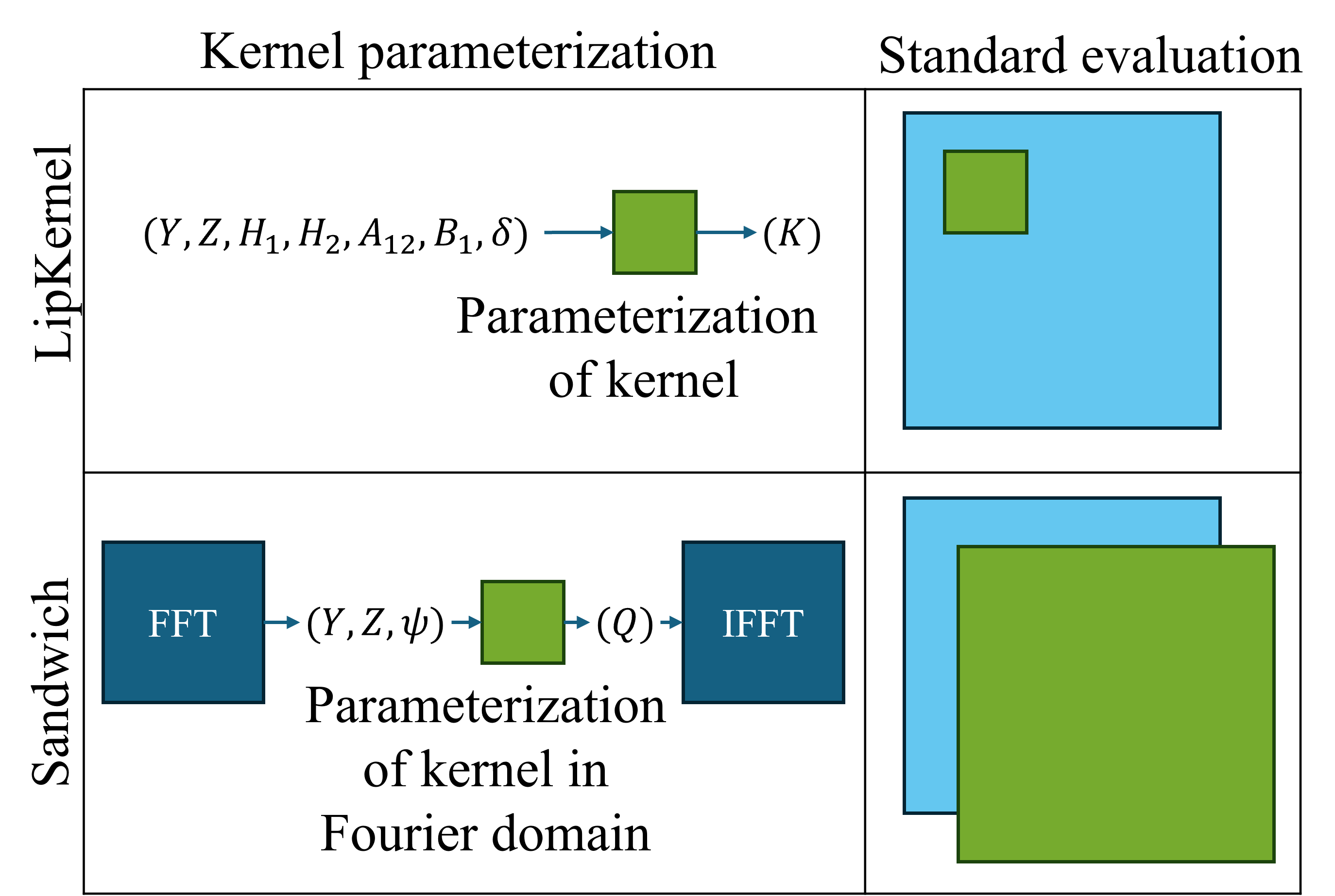
Figure 3: Differences between convolutional layers using LipKernel (ours) and Sandwich layers [20] in its parameterization complexity and its standard evaluation. The light blue boxes represent images and the green boxes the kernel.

In this section, we have presented an LMI-based method for the parameterization of Lipschitz-bounded CNNs that we call LipKernel as we directly parameterize the kernel parameters. Similarly, the parameterization of Sandwich layers [20] is based on LMIs, i.e., is also shows an increased expressivity over approaches using orthogonal layers and layers with constrained spectral norms, cmp. Subsection III-A. In the following, we point out the differences between Sandwich and LipKernel convolutional layers, which are also illustrated in Fig. 3.

Both parameterizations Sandwich and LipKernel use the Cayley transform and require the computation of inverses at training time. However, LipKernel parameterizes the kernel parameters $K$ directly through the bijective mapping $(\boldsymbol{A},\boldsymbol{B},\boldsymbol{C},\boldsymbol{D})\mapsto K$ given by Lemma 1. This means that after training at inference time, we can construct $K$ from $(\boldsymbol{A},\boldsymbol{B},\boldsymbol{C},\boldsymbol{D})$ and then evaluate the trained CNN using this $K$. This is not possible using Sandwich layers [20]. At inference time Sandwich layers can either be evaluated using an full-image size kernel or in the Fourier domain, cmp. Fig. 3. The latter requires the use of a fast Fourier transform and an inverse fast Fourier transform and the computation of inverses at inference time, making it computationally more costly than the evaluation of LipKernel layers.

We note that Sandwich requires circular padding instead of zero padding and the implementation of [20] only takes input image sizes of the specific size of $2^{n}$, $n\in\mathbb{N}_{0}$. In this respect, LipKernel is more versatile than Sandwich and it can further handle all kinds of zero-padding and accounts for pooling layers, which are not considered in [20].

V Numerical Experiments

V-A Run-times for inference

First, we compare the run-times at inference, i.e., the time for evaluation of a fixed model after training, for varying numbers of channels, different input image sizes and different kernel sizes for LipKernel, Sandwich, and Orthogon layers with randomly generated weights².

• Sandwich: [20] suggest an LMI-based method using the Cayley transform, wherein convolutional layers are parameterized in the Fourier domain using circular padding, cmp. Subsection IV-E.

• Orthogon: This method uses the Cayley transform to parameterize orthogonal layers [22]. Convolutional layers are parameterized in the Fourier domain using circular padding.

The averaged run-times are shown in Fig. 4. For all chosen channel, image, and kernel sizes the inference time of LipKernel is very short (from $<$1ms to around 100ms), whereas Sandwich layer and Orthogon layer evaluations are two to three orders of magnitude slower and increases significantly with channel and image sizes (from around 10ms to over 10s). Kernel size does not affect the run-time of either layer significantly.

A particular motivation of our work is to improve the robustness of NNs for use in real-time control systems. In this context, these inference-time differences can have a significant impact, both in terms of achievable sample rates (100Hz vs 0.1Hz) and latency in the feedback loop. Furthermore, it is increasingly the case that compute (especially NN inference) consumes a significant percentage of the power in mobile robots and other “edge devices” [41]. Significant reductions in inference time for robust NNs can therefore be a key enabler for use especially in battery-powered systems.

Figure 4: Inference times for LipKernel, Sandwich, and Orthogon layers with different number of channels $c=c_{\mathrm{in}}=c_{\mathrm{out}}$, input image sizes $N=N_{1}=N_{2}$ and kernel sizes $k=k_{1}=k_{2}$. For all layers, we have stride equal to $1$ and average the run-time over 10 different initializations.

V-B Accuracy and robustness comparison

We next compare LipKernel to three other methods developed to train Lipschitz-bounded NNs in terms of accuracy and robustness. In particular, we compare LipKernel to Sandwich and Orthogon as well as vanilla and almost-orthogonal Lipschitz (AOL) NNs:

• Vanilla: Unconstrained neural network.

• AOL: [14] introduce a rescaling-based weight matrix parametrization to obtain AOL layers which are 1-Lipschitz. Just like LipKernel layers, at inference, convolutional AOL layers can be evaluated in standard form.

We train classifying CNNs on the MNIST dataset [42] of size $32\times 32$ images, using two different CNN architectures, 2C2F: $c(16,4,2).c(32,4,2).f(100).f(10)$, 2CP2F: $c(16,4,1).p(\mathrm{av},2,2).c(32,4,1).p(\mathrm{av},2,2).f(100).f(10)$, wherein by $c(C,K,S)$, we denote a convolutional layer with $C$ output channels, kernel size $K$, and stride $S$, by $f(N)$ a fully-connected layer with $N$ output neurons, and by $p(\text{type},K,S)$ a pooling layer of type “$\mathrm{av}$” or “$\mathrm{max}$”.

In Table I, we show the test accuracy on unperturbed test data, the certified robust accuracy, and the robustness under the $\ell_{2}$ projected gradient descent (PGD) adversarial attack of the trained NNs. The certified robust accuracy is a robustness metric for NNs that computes the minimal margin for each data point and based on the NN’s Lipschitz constant gives guarantees on the robustness to perturbations from an $\epsilon$ ball. The $\ell_{2}$ PGD attack is a white box multi-step attack that modifies each input data point by maximizing the loss within an $\ell_{2}$ $\epsilon$-ball around that point [43].

First, we note that LipKernel is general and flexible in the sense that we can use it in both the 2C2F and the 2CP2F architectures, whereas Sandwich and Orthogon are limited to image sizes of $2^{n}$ and to circular padding and AOL does not support strided convolutions. Comparing LipKernel to Orthogon and AOL, we notice better expressivity in the higher clean accuracy and significantly better robustness with the stronger Lipschitz bounds of 1 and 2. In comparison to Sandwich, LipKernel achieves comparable but slightly lower expressivity and robustness. However as discussed above it is more flexible in terms of architecture and has a significant advantage in terms of inference times.

In Figure 5, we plot the achieved clean test accuracy over the Lipschitz lower bound for 2C2F and 2CP2F for LipKernel and the other methods, clearly recognizing the trade-off between accuracy and robustness. Again, we see that LipKernel shows better expressivity than Orthogon and AOL and similar performance to Sandwich.

TABLE I: Empirical lower Lipschitz bounds, clean accuracy, certified robust accuracy and adversarial robustness under $\ell_{2}$ PGD attack for vanilla, AOL, Orthogon, Sandwich, and LipKernel NNs using the architectures 2C2F and 2CP2F with ReLU activations, each trained for 20 epochs and averaged for three different initializations.

Model	Method	Cert. UB	Emp. LB	Test acc.	Cert. robust acc.			$\ell_{2}$ PGD Adv. test acc.
					$\epsilon=\frac{36}{255}$	$\epsilon=\frac{72}{255}$	$\epsilon=\frac{108}{255}$	$\epsilon=1.0$	$\epsilon=2.0$	$\epsilon=3.0$
2C2F	Vanilla	–	221.7	99.0%	0.0%	0.0%	0.0%	69.5%	61.9%	59.6%
	Orthogon	1	0.960	94.6%	92.9%	91.0%	88.3%	83.7%	65.2%	60.4%
	Sandwich	1	0.914	97.3%	96.3%	95.2%	93.8%	90.5%	76.5%	72.0%
	LipKernel	1	0.952	96.6%	95.6%	94.3%	92.6%	88.3%	72.2%	67.8%
	Orthogon	2	1.744	97.7%	96.3%	94.4%	91.8%	89.1%	66.0%	58.2%
	Sandwich	2	1.703	98.9%	98.2%	97.0%	95.4%	93.1%	74.0%	67.2%
	LipKernel	2	1.703	98.2%	97.1%	95.6%	93.6%	89.8%	66.1%	58.9%
	Orthogon	4	2.894	98.8%	97.4%	94.4%	88.6%	89.6%	56.0%	46.0%
	Sandwich	4	2.969	99.3%	98.4%	96.9%	93.6%	92.5%	63.3%	54.0%
	LipKernel	4	3.110	98.9%	97.5%	95.3%	91.3%	88.6%	49.6%	39.7%
2CP2F	Vanilla	–	148.0	99.3%	0.0%	0.0%	0.0%	73.2%	56.2%	53.7%
	AOL	1	0.926	88.7%	85.5%	81.7%	77.2%	70.6%	49.2%	44.6%
	LipKernel	1	0.759	91.7%	88.0%	83.1%	77.3%	77.3%	57.2%	52.2%
	AOL	2	1.718	93.0%	89.9%	85.9%	80.4%	75.8%	46.6%	38.1%
	LipKernel	2	1.312	94.9%	91.1%	85.4%	77.8%	80.9%	53.8%	45.8%
	AOL	4	2.939	95.9%	92.4%	86.2%	76.3%	78.2%	37.0%	29.6%
	LipKernel	4	2.455	97.1%	93.7%	87.2%	75.7%	80.0%	36.8%	29.0%

Figure 5: Robustness accuracy trade-off for 2C2F (left) 2CP2F (right) for NNs averaged over three initializations.

VI Conclusion

We have introduced LipKernel, an expressive and versatile parameterization for Lipschitz-bounded CNNs. Our parameterization of convolutional layers is based on a 2-D state space representation of the Roesser type that, unlike parameterizations in the Fourier domain, allows to directly parameterize the kernel parameters of convolutional layers. This in turn enables fast evaluation at inference time making LipKernel especially useful for real-time control systems. Our parameterization satisfies layer-wise LMI constraints that render the individual layers incrementally dissipative and the end-to-end mapping Lipschitz-bounded. Furthermore, our general framework can incorporate any dissipative layer.

References

• [1] Y. LeCun, Y. Bengio, and G. Hinton, “Deep learning,” nature, vol. 521, no. 7553, pp. 436–444, 2015.
• [2] C. M. Bishop, “Neural networks and their applications,” Review of scientific instruments, vol. 65, no. 6, pp. 1803–1832, 1994.
• [3] Z. Li, F. Liu, W. Yang, S. Peng, and J. Zhou, “A survey of convolutional neural networks: analysis, applications, and prospects,” IEEE Transactions on Neural Networks and Learning Systems, vol. 33, no. 12, pp. 6999–7019, 2021.
• [4] C. Szegedy, W. Zaremba, I. Sutskever, J. Bruna, D. Erhan, I. Goodfellow, and R. Fergus, “Intriguing properties of neural networks,” arXiv:1312.6199, 2013.
• [5] A. Virmaux and K. Scaman, “Lipschitz regularity of deep neural networks: analysis and efficient estimation,” Advances in Neural Information Processing Systems, vol. 31, 2018.
• [6] P. L. Combettes and J.-C. Pesquet, “Lipschitz certificates for layered network structures driven by averaged activation operators,” SIAM Journal on Mathematics of Data Science, vol. 2, no. 2, pp. 529–557, 2020.
• [7] M. Fazlyab, A. Robey, H. Hassani, M. Morari, and G. Pappas, “Efficient and accurate estimation of Lipschitz constants for deep neural networks,” Advances in Neural Information Processing Systems, vol. 32, 2019.
• [8] F. Latorre, P. Rolland, and V. Cevher, “Lipschitz constant estimation of neural networks via sparse polynomial optimization,” in International Conference on Learning Representations, 2020.
• [9] M. Jordan and A. G. Dimakis, “Exactly computing the local Lipschitz constant of ReLU networks,” in Advances in Neural Information Processing Systems, 2020, pp. 7344–7353.
• [10] M. Revay, R. Wang, and I. R. Manchester, “A convex parameterization of robust recurrent neural networks,” IEEE Control Systems Letters, vol. 5, no. 4, pp. 1363–1368, 2020.
• [11] P. Pauli, D. Gramlich, and F. Allgöwer, “Lipschitz constant estimation for 1d convolutional neural networks,” in Learning for Dynamics and Control Conference.   PMLR, 2023, pp. 1321–1332.
• [12] ——, “Lipschitz constant estimation for general neural network architectures using control tools,” arXiv:2405.01125, 2024.
• [13] C. Anil, J. Lucas, and R. Grosse, “Sorting out Lipschitz function approximation,” in International Conference on Machine Learning.   PMLR, 2019, pp. 291–301.
• [14] B. Prach and C. H. Lampert, “Almost-orthogonal layers for efficient general-purpose Lipschitz networks,” in Computer Vision–ECCV 2022: 17th European Conference, 2022.
• [15] P. Pauli, A. Koch, J. Berberich, P. Kohler, and F. Allgöwer, “Training robust neural networks using Lipschitz bounds,” IEEE Control Systems Letters, vol. 6, pp. 121–126, 2021.
• [16] P. Pauli, N. Funcke, D. Gramlich, M. A. Msalmi, and F. Allgöwer, “Neural network training under semidefinite constraints,” in 61st Conference on Decision and Control.   IEEE, 2022, pp. 2731–2736.
• [17] H. Gouk, E. Frank, B. Pfahringer, and M. J. Cree, “Regularisation of neural networks by enforcing Lipschitz continuity,” Machine Learning, vol. 110, pp. 393–416, 2021.
• [18] M. Revay, R. Wang, and I. R. Manchester, “Lipschitz bounded equilibrium networks,” arXiv:2010.01732, 2020.
• [19] ——, “Recurrent equilibrium networks: Flexible dynamic models with guaranteed stability and robustness,” IEEE Transactions on Automatic Control, 2023.
• [20] R. Wang and I. Manchester, “Direct parameterization of Lipschitz-bounded deep networks,” in International Conference on Machine Learning.   PMLR, 2023, pp. 36 093–36 110.
• [21] P. Pauli, R. Wang, I. R. Manchester, and F. Allgöwer, “Lipschitz-bounded 1D convolutional neural networks using the Cayley transform and the controllability Gramian,” in 62nd Conference on Decision and Control.   IEEE, 2023, pp. 5345–5350.
• [22] A. Trockman and J. Z. Kolter, “Orthogonalizing convolutional layers with the cayley transform,” in International Conference on Learning Representations, 2021.
• [23] R. Roesser, “A discrete state-space model for linear image processing,” IEEE Transactions on Automatic Control, vol. 20, no. 1, 1975.
• [24] D. Gramlich, P. Pauli, C. W. Scherer, F. Allgöwer, and C. Ebenbauer, “Convolutional neural networks as 2-d systems,” arXiv:2303.03042, 2023.
• [25] P. Pauli, D. Gramlich, and F. Allgöwer, “State space representations of the Roesser type for convolutional layers,” arXiv:2403.11938, 2024.
• [26] S. Singla, S. Singla, and S. Feizi, “Improved deterministic l2 robustness on CIFAR-10 and CIFAR-100,” in International Conference on Learning Representations, 2022.
• [27] R. T. Chen, J. Behrmann, D. K. Duvenaud, and J.-H. Jacobsen, “Residual flows for invertible generative modeling,” Advances in Neural Information Processing Systems, vol. 32, 2019.
• [28] J. Behrmann, W. Grathwohl, R. T. Chen, D. Duvenaud, and J.-H. Jacobsen, “Invertible residual networks,” in International conference on machine learning.   PMLR, 2019, pp. 573–582.
• [29] Y. Perugachi-Diaz, J. Tomczak, and S. Bhulai, “Invertible densenets with concatenated lipswish,” Advances in Neural Information Processing Systems, vol. 34, pp. 17 246–17 257, 2021.
• [30] R. Wang, K. Dvijotham, and I. R. Manchester, “Monotone, bi-Lipschitz, and Polyak- Łojasiewicz networks,” in International Conference on Machine Learning.   PMLR, 2024.
• [31] C. I. Byrnes and W. Lin, “Losslessness, feedback equivalence, and the global stabilization of discrete-time nonlinear systems,” IEEE Transactions on Automatic Control, vol. 39, no. 1, pp. 83–98, 1994.
• [32] I. Goodfellow, Y. Bengio, and A. Courville, Deep Learning.   MIT Press, 2016.
• [33] B. Aquino, A. Rahnama, P. Seiler, L. Lin, and V. Gupta, “Robustness against adversarial attacks in neural networks using incremental dissipativity,” IEEE Control Systems Letters, vol. 6, pp. 2341–2346, 2022.
• [34] M. Fazlyab, M. Morari, and G. J. Pappas, “Safety verification and robustness analysis of neural networks via quadratic constraints and semidefinite programming,” IEEE Transactions on Automatic Control, 2020.
• [35] V. V. Kulkarni and M. G. Safonov, “Incremental positivity nonpreservation by stability multipliers,” IEEE Transactions on Automatic Control, vol. 47, no. 1, pp. 173–177, 2002.
• [36] B.-Z. Guo and H. Zwart, “On the relation between stability of continuous-and discrete-time evolution equations via the cayley transform,” Integral Equations and Operator Theory, vol. 54, pp. 349–383, 2006.
• [37] K. Helfrich, D. Willmott, and Q. Ye, “Orthogonal recurrent neural networks with scaled Cayley transform,” in International Conference on Machine Learning.   PMLR, 2018, pp. 1969–1978.
• [38] R. Shepard, S. R. Brozell, and G. Gidofalvi, “The representation and parametrization of orthogonal matrices,” The Journal of Physical Chemistry A, vol. 119, no. 28, pp. 7924–7939, 2015.
• [39] B. Anderson, P. Agathoklis, E. Jury, and M. Mansour, “Stability and the matrix lyapunov equation for discrete 2-dimensional systems,” IEEE Transactions on Circuits and Systems, vol. 33, no. 3, pp. 261–267, 1986.
• [40] A. Araujo, A. J. Havens, B. Delattre, A. Allauzen, and B. Hu, “A unified algebraic perspective on Lipschitz neural networks,” in International Conference on Learning Representations, 2023.
• [41] Y. Chen, B. Zheng, Z. Zhang, Q. Wang, C. Shen, and Q. Zhang, “Deep learning on mobile and embedded devices: State-of-the-art, challenges, and future directions,” ACM Computing Surveys (CSUR), vol. 53, no. 4, pp. 1–37, 2020.
• [42] Y. LeCun and C. Cortes, “MNIST handwritten digit database,” 2010.
• [43] A. Madry, A. Makelov, L. Schmidt, D. Tsipras, and A. Vladu, “Towards deep learning models resistant to adversarial attacks,” arXiv:1706.06083, 2017.