Pedestrian crash causation analysis near bus stops: Insights from random parameters NB-Lindley models

Abstract

Pedestrian safety near bus stops is a growing concern due to rising injuries and fatalities, underscoring the need to mitigate crash risks and encourage active travel through public transportation in urban corridors. However, existing research has often overlooked the effects of exposure characteristics and bus stop design elements on pedestrian-vehicle crashes, limiting the development of data-driven interventions. This study aims to fill that gap by quantifying the relationship between various features (e.g., bus stop design, traffic, and passenger activity, roadway environment, etc.) and vehicle-pedestrian crashes in Fort Worth, Texas, using the Random Parameters Negative Binomial-Lindley (RPNB-L) model to address the unobserved heterogeneity. By accounting for site-specific variability, the RPNB-L model offers a more nuanced understanding of the factors influencing crash frequency. The analysis covers 596 bus stop sites, integrating crash data from 2018 to 2022 with roadway network and stop design characteristics. Results show that the RPNB-L model outperforms traditional Negative Binomial (NB) and fixed-coefficient NB-L models in capturing variability across sites. Significant predictors of higher pedestrian KABCO crash frequencies include average annual daily traffic (AADT), bus passenger boarding rates, stops located near-side of intersections, mixed-use areas, and the absence of medians, sidewalks, or crosswalks. Additional factors, such as poor lighting, high school numbers, and lower speed limits (e.g., 35 mph), also increase crash frequency. The study applies the Potential for Safety Improvement (PSI) metric to identify high-risk sites and prioritize key corridors for intervention. These findings offer actionable insights to help transportation agencies develop targeted policies and infrastructure improvements, ultimately enhancing pedestrian safety and promoting sustainable public transportation in urban areas.

1 Introduction

Ensuring the safety of pedestrians has become an increasingly urgent challenge in the United States, with recent data showing a significant increase in pedestrian fatalities, even as motor vehicle fatalities have modestly declined. Between 2020 and 2021, pedestrian fatalities increased by 12.54%, and over the two-decade period from 2001 to 2021, raised by 50.74%, while vehicle fatalities decreased by 4.67% (Stewart, 2023). Since 2009, pedestrian fatalities have surged by 59%, underscoring the pressing need for enhanced pedestrian safety measures (Sanchez Rodriguez and Ferenchak, 2024). Texas reflects these national trends: where pedestrian fatalities accounted for 20% of all traffic-related fatalities in 2020 (Stewart, 2023). This pattern continued into 2021; there were 5370 pedestrian-involved crashes, resulting in 843 fatalities and 1467 severe injuries. The vulnerability of pedestrians, who lack physical protection and travel at lower speeds, makes them particularly susceptible to severe injuries or death in collisions (Li et al., 2017; Shinar, 2012). Pedestrians are 1.5 times more likely to suffer fatal injuries in crashes compared to motor vehicle occupants (Beck et al., 2007). Fig. 1 illustrates the growing disparity between pedestrian and motor vehicle fatalities over the period from 2001 to 2021, highlighting the need for targeted pedestrian safety interventions.

Fig. 1.: Pedestrian and motor vehicle fatalities (2001-2021)

The increasing number of pedestrian injuries and fatalities has prompted extensive research on pedestrian crash risks to identify contributing factors and hazardous locations (Xie et al., 2017; Lee et al., 2015). Based on historical crash data, the analysis facilitates the identification of key determinants such as roadway characteristics, environmental conditions, vehicle dynamics, and human factors contributing to pedestrian crashes. The findings from these analyses are instrumental in formulating evidence-based countermeasures to enhance the safety of vulnerable road users, inform the design of transportation infrastructure, and shape policies and regulations to improve road safety (Das et al., 2019). While the majority of the existing literature focuses on pedestrian crashes at the intersection (Haleem et al., 2015) or mid-block (Toran Pour et al., 2017; Quistberg et al., 2015a). While these comprehensive insights remain under-explored: pedestrian safety near bus stops.

Bus stops pose unique safety risks, as pedestrians often engage in unsafe behaviors, such as rushing across the street to catch a bus, resulting in increased pedestrian-vehicle interactions (Yendra et al., 2024). The placement of bus stops, whether midblock or near intersections, also influences pedestrian safety (Hu and Cicchino, 2018), with urban arterials often becoming high-risk zones due to increased pedestrian traffic (Clifton and Kreamer-Fults, 2007). According to Campbell et al. (2003), around 2% of all urban pedestrian crashes occur near bus stops. The Highway Safety Manual (2010) also reports that the presence of even one or two bus stops within 1,000 feet of an intersection raises the risk of pedestrian crashes by 2.78 times, escalating to 4.15 times when more than two stops are present. The risks are further amplified by the growing number of larger motor vehicles, which have worsened pedestrian safety outcomes over time (Tyndall, 2021). Therefore, urban arterials with high bus stop numbers increase pedestrian exposure to traffic, heightening the risk of collisions (Hess et al., 2004). These corridors have become focal points for concern (Craig et al., 2019; Ulak et al., 2021), a challenge consistently highlighted in previous studies. Despite these findings, there remains a notable research gap; limited studies focused on crash frequency models on pedestrian crashes near bus stops.

Although a clear connection exists between proximity to bus stops and increased pedestrian crash risks, there remains a lack of focused research on these specific locations. Several gaps in the literature remain unresolved. First, prior studies have largely focused on pedestrian crashes at the intersection and midblock, often using bus stop locations as an explanatory variable. However, few studies have comprehensively analyzed the effects of exposure characteristics and bus stop design elements on pedestrian-vehicle crashes near bus stops. Additionally, there is no established safety performance functions (SPF) framework for bus stops within transit corridors, which is essential for assessing and mitigating crash risks in urban areas. Moreover, limited research has investigated the identification of hazardous bus transit corridors or hotspot locations that elevate pedestrian crash risks. Identifying these high-risk corridors can provide valuable insights, enabling transportation agencies to implement countermeasures that reduce pedestrian crashes. This research addresses these gaps by focusing on the following objectives:

1. Develop SPFs for bus stops within transit corridors, incorporating factors such as exposure, roadway design, and bus stop design elements.

2. Identify and analyze key contributors to pedestrian crashes near bus stops.

3. Identify hazardous bus transit corridors using the Potential for Safety Improvement (PSI) methodology.

To achieve these objectives, this study employs advanced statistical methods to account for the complex nature of pedestrian crashes at bus stops. The Random Parameters Negative Binomial-Lindley (RPNB-L) model addresses unobserved heterogeneity and captures variability in crash frequency across different locations. This model offers a more nuanced understanding of the factors influencing crash risks compared to traditional models. The analysis uses data from 596 bus stop locations in Fort Worth, Texas, integrating crash records from 2018 to 2022 with roadway network and stop design features. Baseline models, including the Negative Binomial (NB) and Negative Binomial-Lindley (NB-L) distributions, are developed for comparison, with the RPNB-L model demonstrating superior performance. This study also applies the PSI metric to identify high-risk sites and corridors, providing transportation agencies with actionable insights to guide policy decisions and infrastructure improvements. Bridging these critical research gaps, this study offers a new framework for improving pedestrian safety within transit corridors.

The structure of this study is organized as follows: Section 2 provides an extensive review of the relevant literature. Section 3 covers the data description. Section 4 describes the methodology, model estimation process, inference, and validation. The model estimation results, along with a brief discussion, are presented in Section 5. Section 6 summarizes the key points and presents the conclusions.

2 Background

Bus stops are critical interaction points where pedestrians, cyclists, bus drivers, car drivers, and other motorists converge, increasing the likelihood of crashes (Torbic et al., 2010). Vulnerable road users, such as pedestrians and bus passengers, face significant safety risks around bus stops (Zhang et al., 2023). A study reported that 89% of high-crash locations are within 150 feet of a bus stop, with 90% within 70 feet of a crosswalk (Walgren, 1998).

Several methods have been employed to analyze pedestrian safety near bus stops, including crash data analysis (Craig et al., 2019; Hess et al., 2004), geography information system-based safety inspections (Yu, 2024), road user observations (Akintayo and Adibeli, 2022), and traffic conflict techniques (Zhang et al., 2023). These approaches require a comprehensive understanding of factors influencing pedestrian safety, including exposure-related behaviors, roadway conditions, bus stop design elements (Clifton et al., 2009; Craig et al., 2019; Haleem et al., 2015; Hu and Cicchino, 2018; Zahabi et al., 2011; Zegeer and Bushell, 2012). However, little attention has been given to bus stop design characteristics and their nearby roadway environment, this oversight may lead to misleading conclusions about the effects of certain variables.

Pedestrian activity increases near bus stops, particularly in high-traffic areas like schools and commercial zones, which heightens the risk of collisions (Geedipally, 2021; Craig et al., 2019; Hess et al., 2004). Risky pedestrian behaviors, such as crossing against signals or boarding buses as they depart, further contribute to crash risks (Quistberg et al., 2015b). Additionally, pedestrians often fail to use crosswalks, increasing the potential for crashes (Pessaro et al., 2017). One study found that 59% of pedestrian crashes occurred when individuals rushed to catch a bus (Wretstrand et al., 2014). Furthermore, waiting in undesignated areas can also cause buses to stop improperly, increasing crash risk (Chand and Chandra, 2017). In light of these behaviors, the number of passengers boarding and alighting at a stop serves as a key indicator of pedestrian activity and is closely linked to crash frequency near bus stops.

Bus stop sign infrastructure plays an essential role in pedestrian safety. Clear and visible signage ensures pedestrians wait in designated areas and signals to bus drivers where to stop. When signs are obstructed by trees or advertisements, the area becomes more dangerous (Rossetti et al., 2020). Additionally, bus shelters are essential for providing accessible waiting spaces, and the absence of such shelters has been identified as a key factor contributing to the riskiest bus stop locations (Salum et al. 2024). These risks are further exacerbated by inadequate pedestrian infrastructure, such as marked crosswalks or pedestrian signals (Pulugurtha and Vanapalli, 2008). Several studies underscore the importance of lighting for safety at bus stops, especially at nighttime (Rossetti et al., 2020; Mukherjee et al., 2023), with poor lighting linked to higher pedestrian fatality rates, especially in sparsely populated areas (Lakhotia et al., 2020). Many studies recommend improved lighting at bus stops and their approaches to enhance safety (Salum et al., 2024; Pessaro et al., 2017).

The risk of pedestrian crashes near bus stops may result in factors like added distraction and poor yielding behavior (Craig et al., 2019). Fitzpatrick and Nowlin (1997) studied the impact of bus stop locations on safety. Far-side bus stops, positioned after an intersection, experience fewer crashes than near-side stops due to fewer conflict points with right-turning vehicles. However, far-side stops can block intersections during peak hours, reducing visibility for both drivers and pedestrians (Institute and Foundation, 1996).

Studies indicate that providing safe and accessible sidewalks near bus stops is strongly correlated with encouraging pedestrian access to bus stops (Sukor and Fisal, 2020). In the absence of designated sidewalks, pedestrians are compelled to walk on roadways, thereby increasing their exposure to traffic and the risk of collisions (Rossetti et al., 2020). Additionally, crosswalks improve safety (Ulak et al., 2021), yet more than 30% of bus stops lack them, making these areas unsafe (Tiboni and Rossetti, 2013). Studies show that a significant proportion of pedestrian crashes occur when individuals do not use crosswalks, with two-thirds of pedestrian fatalities occurring in such situations (Clifton et al., 2009). Moreover, at unsignalized intersections, the severity of pedestrian injuries is significantly influenced by crosswalks ((Clifton et al., 2009)

TThe Safety Performance Function (SPF) is a critical tool in safety research, relating crash frequency to explanatory variables such as traffic characteristics, roadway design, and land use features (Thakali et al., 2015). Research indicates that proximity to signalized intersections near bus stops increases the likelihood of pedestrian crashes, with pedestrian volume and the number of transit stops positively correlated with crash rates (Pulugurtha and Sambhara, 2011). Several studies reinforce this association, emphasizing that bus stops near intersections pose heightened pedestrian risks (Harwood et al., 2008; Kuşkapan et al., 2022; Walgren, 1998). Zeeger & Bushell (2012) found that the likelihood of pedestrian crashes increases significantly when bus stops are located within 1,000 feet of an intersection, especially when combined with high traffic and pedestrian volumes, multiple lanes without a median, and nearby schools. Similarly, Torbic et al. (2010) developed a method to predict vehicle-pedestrian crashes, showing that crashes are four times more likely when a bus stop is within 1,000 feet of a signalized intersection, particularly when schools or alcohol retail stores are present.

Many studies have explored the relationship between the built environment, traffic characteristics, and crash frequency, focusing on factors such as traffic volumes, speed, and geometric features (Hess et al., 2004; Ulak et al., 2021; Lakhotia et al., 2020; Tiboni and Rossetti, 2013). For example, high average annual daily traffic (AADT) near bus stops increases the potential for conflicts between vehicles and pedestrians. Additionally, high traffic speeds are a significant safety risk, especially in urban areas where pedestrian collisions are more frequent (Rossetti et al., 2020). Studies further link bus stops on high-speed roads to increased pedestrian fatalities (Hess et al., 2004; Lakhotia et al., 2020; Pulugurtha and Vanapalli, 2008).

Roadway width also influences pedestrian safety, with wider roads increasing crash risks by making pedestrian crossings more difficult, while narrower roads can lead to more pedestrian-vehicle conflicts (Zhang et al., 2023). The presence of a median near bus stops enhances safety by providing pedestrians with a refuge area, allowing them to cross one direction of traffic at a time (Pessaro et al., 2017). Median islands further reduce collision risks by improving crossing safety (Yu, 2024). Land use also plays a crucial role in pedestrian safety near bus stops. High-activity areas, such as shopping centers, schools, and workplaces, attract significant pedestrian and vehicular traffic, increasing collision risks (Hess et al., 2004). Areas with high vehicular activity, particularly commercial zones like big box stores, are associated with more pedestrian crashes due to increased traffic flow and parking-related movements (Yu, 2024).

Several researchers have conducted investigations pertaining to the identification of hotspots with a high incidence of pedestrian-vehicle collisions, as well as the identification of bus stops that pose safety risks (Truong and Somenahalli, 2011; Ulak et al., 2021). Truong & Somenahalli (2011) proposed a GIS approach that used spatial autocorrelation analysis and severity indices to analyze and rank unsafe bus stops based on pedestrian-vehicle crash data. Ulak et al. (2021) introduced the Bus Stop Safety Index (SSI) as a quantitative measure of pedestrian safety around bus stops. This SSI identifies high-risk bus stops based on injury severities, spatial distance to pedestrian-involved crashes, socio-demographic factors, traffic indicators, proximity to facilities, and bus stop metrics in Palm Beach County, FL. The Bus Stop Safety Index prioritizes high-risk bus stops to facilitate targeted efforts in enhancing pedestrian safety, making it a valuable tool for improving the safety and accessibility of urban transit systems.

While previous studies have recognized the importance of bus stops in pedestrian safety, none have provided a comprehensive methodology to assess the combined influence of roadway environments and bus stop characteristics on crash risks. Most studies treat bus stops as secondary explanatory variables without thoroughly examining how infrastructure, traffic, and environmental factors interact to influence crash frequency. To address this gap, the current study develops an SPF model that integrates multiple variables to quantify crash risks and identify hazardous transit corridors. By using advanced statistical models, the study aims to provide actionable insights that can guide transportation agencies in implementing targeted interventions to enhance pedestrian safety near bus stops.

3 Data description

This section provides an overview of the data sources and key variables used in this study. Subsection 3.1 introduces the pedestrian crash data obtained from the Texas Department of Transportation’s (TxDOT) Crash Records Information System (CRIS) database. Subsection 3.2 describes the additional data collected on bus stop design elements, missing roadway attributes, and exposure-related features, which complement the crash data to offer a comprehensive view of the factors influencing pedestrian safety near bus stops

3.1 Pedestrian crash data

The study utilized bus stop data from the Fort Worth-area transit service, Trinity Metro, accessed from their official website at https://www.trinitymetro.org. Trinity Metro provided Geographic Information Systems (GIS) shapefiles of bus routes and stops, including details about amenities and wheelchair accessibility at each stop. The dataset encompassed 2,500 bus stops, each identified by the main street and nearby cross-street. Additionally, two spreadsheets with boarding and alighting data were provided, categorized by stop and day type (weekday, Saturday, Sunday) for two time periods: pre-pandemic (September 2019) and during the pandemic (September 2021).

Pedestrian crash data from TxDOT’s Crash Records Information System (CRIS) database covered the years 2018 to 2022 (see: Table 1). Only TxDOT reportable crashes those involving fatalities, injuries, or property damage exceeding $1,000 on public roadways were included. A 250-foot radius around each bus stop was used to extract relevant pedestrian crash data, focusing specifically on crashes occurring on the same roadway as the bus stop. Crashes within the radius but on a nearby cross-street were manually reviewed and excluded. Given the challenge of collecting safety data for every bus stop, the study sampled bus stop locations to gather data effectively.

Once the crash data was obtained, two categories of bus stops were identified:

1. Bus stops with at least one pedestrian crash during the study period.

2. Bus stops with no crash history but high daily passenger activity (more than 75 passengers).

Fig. 3.1 provides a flowchart of the data preparation process, detailing each step undertaken in the study.

Table 1: Records of CRIS data (Few columns)

Stop ID	Total On	Crash Date	Time	Speed	Weather	Light Con.	Surface Con.	Day	Lane Num.	Median	Severity
719	25	4/27/2018	7:36:00 PM	45	CLEAR	DARK, LIGHTED	DRY	FRI	6	CURBED	B
641	44.9	4/23/2019	8:06:00 PM	40	CLOUDY	DARK, NOT LIGHTED	WET	TUE	6	NO MEDIAN	C
743	4.9	3/23/2018	8:06:00 AM	40	CLEAR	DARK, LIGHTED	DRY	FRI	6	UNPROTECTED	K
658	316.1	9/1/2019	3:00:00 AM	40	CLEAR	DARK, LIGHTED	DRY	WED	4	NO MEDIAN	A
757	10.2	2/3/2020	9:27:00 PM	35	RAIN	DARK, LIGHTED	WET	MON	6	CURBED	B
642	27.2	8/9/2020	4:00:00 PM	40	CLEAR	DAYLIGHT	DRY	WED	6	CURBED	K
.	.	.	.	.	.	.	.	.	.	.	.
.	.	.	.	.	.	.	.	.	.	.	.
.	.	.	.	.	.	.	.	.	.	.	.
131	47.1	3/26/2021	5:36:00 PM	45	CLEAR	DAYLIGHT	DRY	FRI	4	NO MEDIAN	C
757	10.2	11/26/2021	5:51:00 PM	40	CLEAR	DARK, LIGHTED	DRY	FRI	6	CURBED	K
746	9.2	8/5/2022	10:09:00 PM	45	CLEAR	DARK, LIGHTED	DRY	FRI	6	CURBED	B
589	37	12/8/2022	5:15:00 PM	45	CLOUDY	DARK, NOT LIGHTED	WET	THU	6	CURBED	B
.	.	.	.	.	.	.	.	.	.	.	.
.	.	.	.	.	.	.	.	.	.	.	.

Fig. 2.: Flowchart for data preparation

To ensure a reliable sample size for developing the safety prediction model, 596 bus stop locations were selected, as shown in Fig. 3.1. To complement the crash data with traffic and geometric information, the study used TxDOT’s 2019 Roadway Highway Inventory Network Offload (RHiNo) database. This comprehensive database contains details on roadway design and traffic characteristics for both state and local roads, including historical traffic volumes from the past ten years.

The RHiNo database, provided in GIS format, enabled seamless integration with bus stop information. It includes essential data, such as roadway segment location, system type, facility type, design characteristics (e.g., number of lanes, surface width, shoulder width, and median type), and current and historical traffic volumes. When geometric data were missing from the RHiNo database, such as sidewalk presence, crosswalk, or lighting conditions, the study used Google Earth® and Google Street View® to fill in the gaps. These tools proved to be valuable resources for collecting additional geometric information.

Fig. 3.: Bus stop locations for data collection in Fort Worth

The pedestrian crash dataset contains 448 recorded crashes, categorized by severity. Of these, 46 crashes (10.3%) resulted in fatalities (K), meaning the pedestrian was killed in the incident. Another 394 crashes (87.8%) involved injuries (A, B, or C levels), with pedestrians sustaining either incapacitating or non-incapacitating injuries. The remaining 8 crashes (less than 2%) were classified as property damage only (O), with no reported injuries. Fig. 3.1 visualizes the yearly distribution of crashes by severity level, and Fig.3.1 illustrate their distribution.

The data underscores the significant risks pedestrians face, with nearly 98% of incidents involving some form of injury or fatality. The relatively small proportion of property damage-only incidents emphasizes the need for enhanced pedestrian safety measures. Even when crashes are non-fatal, pedestrians are frequently harmed, highlighting the critical importance of targeted interventions to reduce both injury-related and fatal outcomes.

Fig. 4.: Yearly different severity levels of pedestrian crashes

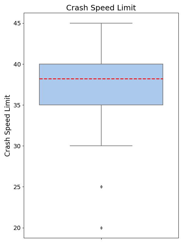
(a)

(b)

(c)

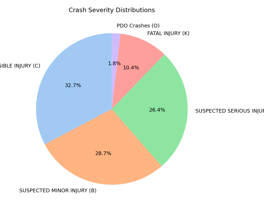
(d)

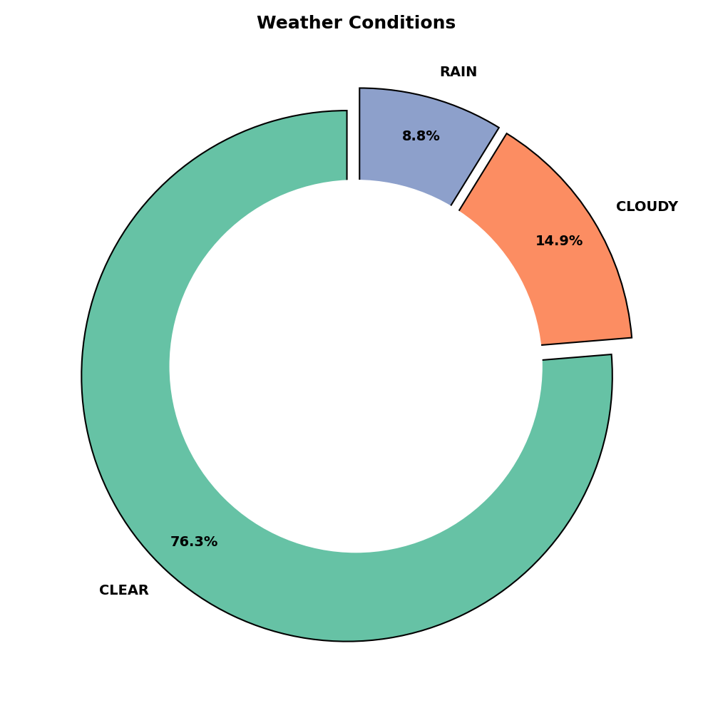
(e)

Fig. 5.: Crash distribution characteristics

3.2 Bus Stops based data

Among the 596 bus stops analyzed, 280 locations, or 46.97%, did not record any pedestrian crashes during the study period. These locations were selected based on specific criteria outlined in the subsection 3.2. As shown in Fig. 3.2, the crash distribution is heavily skewed towards stops with zero recorded crashes. The skewness of the data, calculated at 2.87, indicates significant right skewness, primarily due to the high number of stops without any crashes.

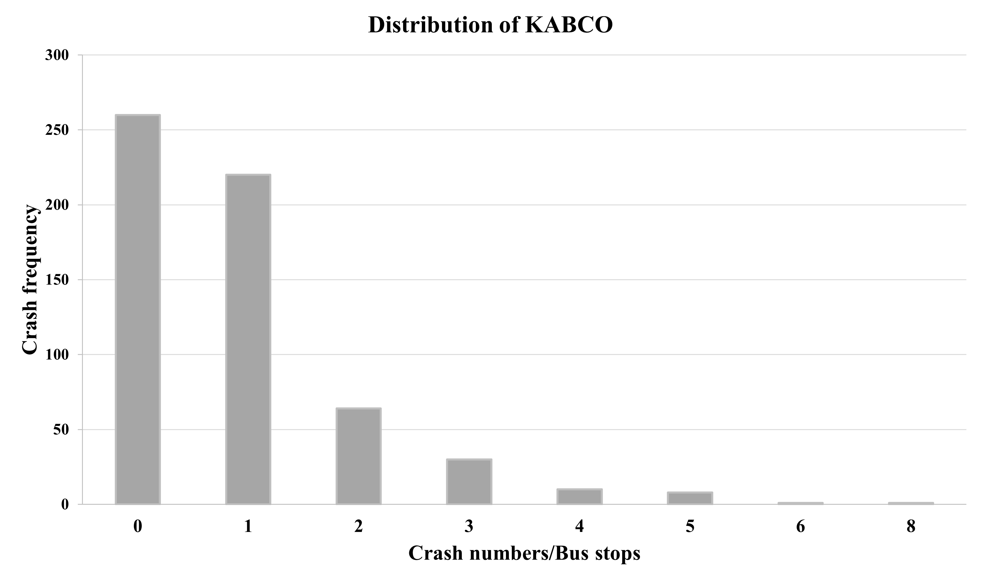
Fig. 6.: KABCO crash distribution

This study distinguishes itself by incorporating a wide range of explanatory variables, capturing spatial and temporal characteristics that are often excluded from traditional Safety Performance Functions (SPFs). Table 2 provides descriptive statistics for the response variables, including the crash data, and other associated explanatory variables. The study draws data from multiple sources: CRIS, RHiNo, Trinity Metro, Google Earth®, and Google Street View® to ensure a comprehensive analysis. The collected variables are organized into categories covering exposure features, bus stop design characteristics, road features, and contextual elements influencing pedestrian safety. Exposure features reflect traffic and pedestrian volumes, providing insights into potential crash risk. Bus stop design characteristics describe the physical attributes of the stops, including their design and proximity to intersections, while road features capture elements of the surrounding roadway, such as lane count, speed limits, and median presence. Contextual elements account for additional factors, such as lighting conditions and land use, that may also affect safety outcomes.

To capture the severity of crashes in a nuanced way, the crash data are classified into three groups. The first group includes total crashes (KABCO), encompassing all pedestrian-involved crashes. The second group focuses on KABC crashes, comprising incidents that resulted in fatalities (K), incapacitating injuries (A), or other injuries (B and C). The third group includes KAB crashes, concentrating on severe incidents involving fatalities and injuries classified as K, A, or B. This classification framework allows for a more detailed investigation into the relationship between crash severity and explanatory variables.

Table 2 presents the descriptive statistics for these variables, highlighting key aspects of the bus stop environments. The mean number of total crashes per bus stop is 0.752, with a maximum of 8 crashes recorded at a single location. KABC crashes have a lower mean of 0.526, with a maximum of 6 crashes, while KAB crashes exhibit a mean of 0.314, with a maximum of 5 crashes. These figures emphasize the variability in crash occurrences across the study area.

The study includes several continuous variables, such as Average Annual Daily Traffic (AADT), which captures traffic exposure near bus stops. AADT ranges from 166 to 42,056 vehicles per day, with a mean of 13,558.2 vehicles. Passenger boarding and alighting volumes provide additional insights into the level of pedestrian activity at each stop, while the distance to the nearest intersection ranges from 0.4 feet to over 2,100 feet, helping to assess spatial relationships between intersections and pedestrian crashes. These continuous variables are complemented by categorical variables, including the presence of signalized intersections, marked crosswalks, and bus stop shelters, each of which may influence pedestrian safety outcomes.

Table 2: Descriptive statistics of variables used for models

Variable	Definition	Descriptive statistics
		Min	Max	Mean	Std Dev
Total crashes	KABCO frequency	0	8	0.752	1.45
KABC crashes	KABC frequency	0	6	0.526	1.11
KAB crashes	KAB frequency	0	5	0.314	0.65
Continuous variables
AADT	Traffic Volume on the street near bus stop	166	42056	13558.2	8828.04
Avg on	Average boarding	0	205.4	11.93	19.79
Avg off	Average alighting	0	215.2	15.24	23.15
Dis to int	Distance between bus stop and nearest intersection corner	0.4	2106	180.60	206.29
Med w	Median width	0.00	131.9	7.10	12.38
Speed limit	Posted speed limit	20	65	36.63	7.95
Lane count	Total number of lanes	1	8	4.34	1.46
School	Number of schools within a half-mile walk of the bus stop	0	4	0.70	0.92
Park count	Number of parks within a half-mile walk of the bus stop	0	6	0.55	0.81
Stop count	Count of transit stops (bus or rail) within a quarter mile of the bus stop	0	11	3.45	2.19
Categorical variables		Category	No of Stops	Crash Frequency
Int t	Nearest intersection type	Signalized (1)	384	237
		Non-signalized (0)	212	206
Marked Xwalk	Presence of marked crosswalk within 250ft of bus stop	No (1)	223	268
		Yes (0)	373	175
Med t	Median types	Undivided (1)	299	267
		Divided (0)	297	176
Lighting	Lighting presence	No (1)	339	273
		Yes (0)	257	170
Area	Area type	Com (0)	332	280
		Res (1)	78	55
		Mix (2)	186	108
Sidewalks	Presence of sidewalks	Yes (0)	550	398
		No (1)	46	45
Curve	Presence of curve near bus stop	Yes (1)	55	40
		No (0)	474	245
Design	Bus stop design	Curbside (1)	507	416
		Other (0)	89	27
Proximity	The proximity of intersection from bus stop location	Far (0)	306	210
		Near (1)	206	166
		Midblock (2)	84	70
Cover	Presence of shelter	Covered (0)	302	236
		Uncovered (1)	294	207

This section emphasizes the diversity and richness of the collected data, which enables detailed exploration of the factors influencing crash frequency and severity across different bus stop locations. By integrating multiple data sources and capturing both quantitative and categorical aspects, the study lays a solid foundation for developing a robust safety prediction model.

4 Methodology

The primary objective of this study is to analyze the relationship between pedestrian crashes and associated risk factors near bus stops, addressing the research gaps identified in the literature review. To achieve this, multiple statistical models were selected based on insights from prior crash frequency modeling studies. This section provides an overview of the selected methodologies and the criteria used to assess model performance. The crash data exhibited characteristics such as excess zeros and significant right skewness. To address the resulting overdispersion, the study applied Negative Binomial (NB) and Negative Binomial-Lindley (NB-L) models. Additionally, the Random Parameters Negative Binomial-Lindley (RPNB-L) model was employed to allow posterior parameter estimates to vary across observations, further reducing modeling errors.

4.1 Feature selection

A critical step in the modeling process involved identifying and eliminating highly correlated variables to improve model efficiency and accuracy. The Pearson correlation coefficient (PCC), shown in Equation 1, was used to measure correlations between variables. If the PCC between two variables exceeded a set threshold, the variable with lower feature importance was removed to prevent multicollinearity. The final set of independent variables included AADT, signalized intersection, cover presence, bus stop count, school count, park count, number of lanes on the street, median width, speed limit, distance from the bus stop to the intersection, median, lighting, area, curve, curb lane for all vehicle types, and curb dedicated to the bus only. The selected variables provide a robust basis for analyzing the complex relationship between pedestrian crashes and associated factors near bus stops.

$${c_{xy}=\frac{\sum_{i=1}^{n}(x_{i}-\bar{x})(y_{i}-\bar{y})}{\sqrt{\sum_{i=1}^{n}(x_{i}-\bar{x})^{2}}\sqrt{\sum_{i=1}^{n}(y_{i}-\bar{y})^{2}}}}$$ (1)

4.2 Models

Developing a Safety Performance Function (SPF) is essential for quantifying the relationship between pedestrian crashes and risk factors, facilitating predictive analysis, and guiding data-driven safety interventions. To achieve this, statistical modeling techniques are commonly applied, where crash frequency serves as the dependent variable and pedestrian characteristics, roadway features, and bus stop design factors function as independent variables. This section provides a concise overview of the methodologies employed in this study. As previously noted, the pedestrian crash data exhibited a high prevalence of zero-crash sites and a strong rightward skew. To account for overdispersion in the data, the generalized linear negative binomial (NB) model with a log link was deemed appropriate. Furthermore, to address the overdispersion stemming from the excess zero-crash observations, the Negative Binomial-Lindley (NB-L) mixed distribution model was employed. Additionally, by allowing the posterior estimates of the explanatory variables to vary across observations, the Random Parameters Negative Binomial-Lindley (RPNB-L) model further reduced modeling errors. The following subsection elaborates on the methodology for estimating the NB, NB-L and RPNB-L models.

4.2.1 Negative Binomial (NB)

The starting point in SPF development is using the Poisson model (Lord et al. 2005). However, this model may not hold true for pedestrian crashes due to over-dispersion in the crash data. The recommended model is the generalized linear negative binomial (NB) model with a log link to account for over-dispersion (Lord and Mannering 2010), thus addressing the requirement that the variance is greater than the mean $\text{Var}(n_{i})>E(n_{i})$. Equations (2)-(4) show the mean frequency $\mu_{i}$, variance, and probability density function of the NB model, respectively.

$$\mu_{i}=\exp(\beta X_{i}+\lambda_{i})$$ (2)

$$\text{Var}(y_{i})=\mu_{i}+\frac{\mu_{i}^{2}}{\phi}$$ (3)

$$P(y_{i})=\left(\frac{\mu_{i}}{\phi+\mu_{i}}\right)^{y_{i}}\left(\frac{\phi}{\phi+\mu_{i}}\right)^{\phi}\frac{\Gamma(\phi+y_{i})}{\Gamma(\phi)\cdot\Gamma(y_{i}+1)}$$ (4)

The traditional negative binomial (NB) model assumes a fixed dispersion parameter $\alpha\left(\alpha=\frac{1}{\phi}\right)$ across all sites. However, several previous studies have demonstrated that this assumption often does not hold true. For instance, Lord and Miranda-Moreno (2008) showed that the dispersion parameter of the NB model is not constant, considering the dispersion parameter $\alpha$ to vary as a function of site-specific characteristics for improved accuracy.

4.2.2 Negative Binomial-Lindley (NB-L)

The NB-L model (Geedipally et al. 2012; Rahman Shaon and Qin 2016) model is an extension of the standard NB model designed to handle highly overdispersed count data. Geedipally et al. (2012) demonstrated that the NB-L model performs better than the NB model when the data contains many zeros or is characterized by a long tail. The NB-L model introduces an additional layer of flexibility by combining the NB distribution with the Lindley distribution to better account for unobserved heterogeneity and excess variation in the data. Therefore, the mixture of the NB and Lindley distributions is as follows:

$$P(Y_{i}=y_{i}|\mu_{i},\phi,\theta)=\int\text{NB}(y_{i}|\phi,\lambda_{i}\mu_{i})\text{Lindley}(\lambda_{i}|\theta)\,d\lambda_{i}$$ (5)

The random error term is represented by $\lambda_{i}$, while the Lindley distribution is denoted by $\theta$. In Equation (5), both $\lambda_{i}$ and $Y_{i}$ are assumed to follow a NB distribution, with the mean defined as $\lambda_{i}\mu_{i}$. The corresponding inverse dispersion parameter is expressed as $\phi=\frac{1}{\alpha}$, where $\lambda_{i}$ is governed by the Lindley distribution parameter $\theta$.

Here, the Lindley distribution can be presented as (Lord et al., 2021) is defined as:

$$\text{Lindley}(x|\theta)=\frac{\theta^{2}}{\theta+1}(1+x)e^{-\theta x},\quad\theta>0,x>0$$ (6)

The mean response function for the NB-L can be expressed as:

$$E(Y_{i}=y_{i})=\mu_{i}\cdot E(\lambda_{i})$$ (7)

Where $\mu_{i}$=$\exp(b_{0}+\sum_{j=1}^{q}b_{j}X_{j})$ represents the expected number of crashes, and $E(\lambda_{i})$ = $\frac{\theta+2}{\theta(\theta+1)}$ is the expected value of the Lindley-distributed term. Replacing the values for $\mu_{i}$ and $E(\lambda_{i})$, the mean response function becomes:

$$E(Y_{i}=y_{i})=\exp\left(b_{0}+\sum_{j=1}^{k}b_{j}X_{j}\right)\cdot\frac{\theta+2}{\theta(\theta+1)}=\exp\left(b_{0}+\log\left(\frac{\theta+2}{\theta(\theta+1)}\right)+\sum_{j=1}^{k}b_{j}X_{j}\right)$$ (8)

To simplify, we incorporate the term $\log\left(\frac{\theta+2}{\theta(\theta+1)}\right)$ into a new intercept term, $b^{\prime}_{0}$, yielding:

$$E(Y_{i}=y_{i})=\exp\left(b^{\prime}_{0}+\sum_{j=1}^{k}b_{j}X_{j}\right)$$ (9)

Where:

$$b^{\prime}_{0}=b_{0}+\log\left(\frac{\theta+2}{\theta(\theta+1)}\right)$$

Thus, the NB-L mean response function accounts for over-dispersion and excess zeros by adjusting the intercept term to include the Lindley distribution’s effects.

The Lindley distribution is a mixture of two Gamma distributions as follows (Zamani and Ismail, 2010):

$$\lambda_{i}\sim\frac{1}{1+\theta}\text{Gamma}(2,\theta)+\frac{\theta}{1+\theta}\text{Gamma}(1,\theta)$$ (10)

The Equation 10 alternatively, it can be restructured as according to Lord et al., 2021

$$\lambda_{i}\sim\sum\left\{\text{Gamma}(1+z_{i},\theta)\text{Bernoulli}\left(z_{i};\frac{1}{1+\theta}\right)\right\}$$ (11)

Therefore, the NB-L model can be written as the following hierarchical model (Geedipally et al., 2012; Lord et al., 2021; Khodadadi et al., 2023):

$$P(Y_{i}=y_{i};\phi,\mu_{i}|\lambda_{i})=\text{NB}(y_{i};\phi,\lambda_{i}\mu_{i})$$ (12)

$$\mu_{i} =\exp\left(b_{0}+\sum_{j=1}^{q}b_{j}X_{j}\right)$$ (13)

$$\lambda_{i} \sim\text{Gamma}(1+z_{i},\theta)$$ (14)

$$z_{i} \sim\text{Bernoulli}\left(\frac{1}{1+\theta}\right)$$ (15)

Prior distributions must be specified to estimate the model parameters using a Bayesian framework. These priors reflect past knowledge or assumptions about the parameters. The random error $\lambda$ term is given a non-informative prior from a gamma distribution, while the gamma shape parameter is governed by a Bernoulli distribution with probability $1/(1+\theta)$. When weakly informative priors are used, the Lindley distribution can potentially exert greater influence on the model compared to the NB component. One challenge in Bayesian estimation is the poor mixing of the MCMC process caused by the correlation between the intercept and the error term. To mitigate this issue, the Geedipally et al., 2012 recommends employing informative priors when possible. A prior should be chosen to ensure that $E(\varepsilon)=1$, which limits the influence of the Lindley distribution. Geedipally et al. (2012) advocate for the use of a prior on $1/(1+\theta)$ that follows a beta distribution, specifically Beta(n/3, n/2), where $n$ represents the number of observations. This approach enhances model stability and improves the accuracy of parameter estimation.

4.2.3 Random Parameters Negative Binomial-Lindley (RPNB-L)

Random parameters (RP) models an alternative way to account for unobserved heterogeneity by allowing parameters to vary from one observation to another (Anastasopoulos and Mannering 2009; Barua et al. 2016; Shaon et al. 2018). To form this randomized variable, lets assume the coefficient $\beta_{ij}$ associated with the $j$-th covariate for the $i$-th site and which can be expressed as:

$$b_{ij}=b_{j}+v_{ij}$$ (16)

where $b_{j}$ represents the fixed mean estimate of the parameter, and $v_{ij}$ is the random term, which typically follows a normal distribution with a mean of zero and a variance of $\sigma^{2}$. This $v_{ij}$ is included in the model if its standard deviation is significantly different from zero; otherwise, a fixed parameter $b_{j}$ is applied uniformly across all observations (El-Basyouny and Sayed, 2009; Anastasopoulos and Mannering, 2009). The probability mass function (pmf) of RPNB model is given by:

As mentioned above, the NB-L model itself is the RP model since it accommodates the Lindley distribution by introducing site-specific effects, which coefficient fully transform to randomized by introducing RPNB-L, meaning that the coefficients of the covariates vary across sites, not just the Lindley portion. This leads to a hierarchical model structure according to Shaon et al., 2018

$$P(Y_{i}=y_{i};\phi,\mu_{i}\mid\lambda_{i}) =\text{NB}(y_{i};\phi,\lambda_{i}\mu_{i})$$

$$\mu_{i} =\exp\left(b_{0}+\sum_{j=1}^{k}b_{ij}X_{ij}\right)$$ (17)

In this hierarchical structure, the random effect $\lambda_{i}$ follows a gamma distribution, $\lambda_{i}\sim(\lambda|1+z_{i},\theta)$, and $z_{i}$ follows a Bernoulli distribution $z_{i}\sim\text{Bernoulli}\left(z|\frac{1}{1+\theta}\right)$. The random parameter $b_{ij}=b_{j}+v_{ij}$ captures site-specific variability, where $v_{ij}\sim\mathcal{N}(0,\sigma_{j}^{2})$.

A known issue with RPNB-L models, especially in a Bayesian framework, is poor mixing of the MCMC chains, particularly due to correlations between the intercept and coefficients, both of which vary across observations. One solution is to standardize the coefficients before using them in the model. After the MCMC chains converge, the standardized coefficients can be transformed back to their original scale using the following transformations for easier interpretation:

$$x_{ij}^{*}=\frac{x_{ij}-\mu_{j}}{\sigma_{j}}$$ (18)

where $\mu_{j}$ and $\sigma_{j}$ are the mean and standard deviation of the $j$-th covariate. After the analysis, the estimated coefficients are transformed back to the original scale using (Gelfand et al., 1995):

$$b_{1}=\frac{b_{1}^{*}}{\sigma_{1}},\quad\dots,\quad b_{q}=\frac{b_{q}^{*}}{\sigma_{q}},\quad b_{0}=b_{0}^{*}-\sum_{j=1}^{q}\frac{b_{j}\mu_{j}}{\sigma_{j}}$$ (19)

The random parameters $w_{ij}$ are modeled using a normal prior:

$$b_{ij}\sim\mathcal{N}(b_{j},\sigma_{j}^{2}),\quad\frac{1}{\sigma_{j}^{2}}\sim\Gamma(0.01,0.01)$$ (20)

Previous research has shown that normal distributions typically provide the best fit for modeling the RP compared (Anastasopoulos and Mannering, 2009) to using lognormal, uniform, gamma, triangular, etc, which helps ensure effective MCMC mixing and improves the robustness of the model’s estimates.

4.3 Model performance

The Deviance Information Criterion (DIC) is widely used within the Bayesian framework for model selection, given the availability of numerous models. The principle of DIC is parsimony, aiming to find the simplest model that explains the most variation in the data. The DIC is calculated as:

$$\text{DIC}=\bar{D}+p_{D}$$ (21)

where $\bar{D}$ is the posterior mean deviance, indicating model fit, and $p_{D}$ is the effective number of parameters. Generally, a model with a lower DIC is preferred. A difference greater than 10 in DIC values between models strongly favors the model with the lower DIC. Differences between 5 and 10 are considered substantial, while differences less than 5 suggest that the models are competitive.

The evaluation process relied on two metrics: Mean Absolute Error (MAE) and Root Mean Square Error (RMSE), to assess the performance of the models on the test set and identify the best combination of hyperparameters for each model. By comparing the performance of all models, we can identify the superior results in capturing the relationship between pedestrian crashes and risk factors (Lord et al. 2021).

The MAE is calculated as:

$$\text{MAE}=\frac{1}{n}\sum\left|y_{\text{observed}}-y_{\text{predicted}}\right|$$ (22)

where $n$ represents the number of observations, and $y_{\text{observed}}$ and $y_{\text{predicted}}$ correspond to the observed and predicted crash counts, respectively.

The RMSE is calculated as:

$$\text{RMSE}=\sqrt{\frac{1}{n}\sum\left(y_{\text{observed}}-y_{\text{predicted}}\right)^{2}}$$ (23)

These metrics are commonly employed to assess the accuracy of the model predictions by comparing the observed and predicted values of crash counts. The MAE provides the average magnitude of the errors in a model’s predictions, while the RMSE gives greater weight to larger errors, offering a more sensitive measure of model performance.

4.4 Marginal effects

The marginal effect of explanatory variables $X_{i}$ on the expected mean value $\mu_{i}$ of $n$ number of crashes is used to quantify the sensitivity of mean crash frequency to changes in these variables. Specifically, the marginal effect describes the extent to which a unit change in an explanatory variable $X_{i}$ leads to a change in the expected mean crash frequency. For explanatory variables that range from 0 to 1, the marginal effect (Washington et al. 2020) can be formulated as follows:

$$\text{ME}_{X_{nm}}={\frac{\partial\mu_{n}}{\partial X_{nm}}}\cdot{\frac{X_{nm}}{\mu_{n}}}=\beta_{nm}\cdot X_{nm}$$ (24)

Where, $\text{ME}_{X_{nm}}$ is defined as the mean marginal effect of the $n$th explanatory variable at the $m$th observation, $\partial\mu_{n}$ denotes the expected mean crash frequency, and $X_{nm}$ is the explanatory variable of interest.

This formulation implies that for a one-unit increase in $X_{nm}$, the expected mean crash frequency $\mu_{n}$ changes proportionally to $\beta_{nm}$, which reflects the relationship between the variable and crash risk (Lord and Mannering 2010). These effects for the NB and NB-L models were calculated using the above formulation. For the RPNB-L model, after MCMC simulations in Openbugs or Multibugs reached convergence, the site-specific parameter means were estimated and subsequently utilized to compute the marginal effects for each observation.

5 Results and Discussion

This section is organized into two parts. The first part describes the model estimation process, and the second part evaluates the models’ performance.

5.1 Model Estimation

Several NB-based (NB, NB-L, RPNB-L) models, were explored using the methodology described earlier. These models included both fixed-coefficient versions (NB and NB-L) and the random parameters NB-L model (RPNB-L) to capture variability in pedestrian crash data more effectively. Each model was estimated and compared within the same Bayesian framework to assess its performance. For the analysis, we employed OpenBUGS to perform the complex computations required for estimating posterior distributions through Markov Chain Monte Carlo (MCMC) algorithms.

Given the bias and auto-correlation inherent in MCMC samples, we ran numerous iterations to mitigate these effects. Multiple simulation chains were executed to ensure robust convergence, each initialized with different starting values. Specifically, three chains were run for 80,000 iterations per parameter, with the first 30,000 samples discarded as burn-in to eliminate potential bias. The remaining 50,000 iterations were used to estimate posterior distributions. Convergence was evaluated by visually inspecting trace plots, which show the progression of chains from various starting points, and by calculating the Brooks-Gelman-Rubin (BGR) statistic for each parameter (El-Basyouny and Sayed 2009). A BGR value stabilized near 1 (below 1.1) indicated effective convergence (Gelman and Rubin 1992; Mitra and Washington 2007). Additionally, the Monte Carlo (MC) error for each parameter was kept below 3% of the posterior standard deviation to ensure reliable parameter estimates.

The dependent variable in this study was the frequency of pedestrian-vehicle crashes near bus stops, with all severity levels included. The explanatory variables were assessed at a 5% significance level, using 95% confidence intervals to identify the significant factors influencing crash frequency. The random parameter approach introduced a hierarchical layer to the Bayesian models, allowing certain parameters to vary across observations. However, if randomization did not meaningfully improve model performance, the parameter was retained as a fixed coefficient to avoid unnecessary model complexity.

In this study, bus stop characteristics and roadway features were treated as fixed parameters, while traffic and pedestrian exposure variables were modeled as random parameters based on the outcomes of the model selection process. This approach allowed the models to balance complexity and performance, ensuring that only parameters with meaningful variability were assigned random effects.

5.2 Model performance evaluation

The RPNB-L model provides 3.27% and 9.21% lower DIC compared to the NB-L and NB models, respectively. The RPNB-L model stands out for its exemplary performance across several key statistical measures used to evaluate model efficacy.

The study evaluated the performance of three models: NB, NB-L, and RPNB-L, with the results presented in Table 3. According to the DIC statistics, the RPNB-L model outperformed both the NB and NB-L models, achieving the lowest DIC value. Specifically, the RPNB-L model’s DIC was 3.27% lower than the NB-L model and 9.21% lower than the NB model, demonstrating also superior performance across other key statistical measures.

The RPNB-L model exhibited the lowest posterior mean deviance (Dbar), indicating a better overall fit than the competing models. This model’s strength lies in its higher effective number of parameters (PD), a result of incorporating mixed distributions and random parameterization. While greater model complexity often carries performance penalties, the RPNB-L model enhances data fit without compromising accuracy. In fact, it is evidenced by the minimal deviance and the lowest DIC value. Therefore, despite the inherent penalties associated with increased complexity, the RPNB-L model’s superior fit and reduced deviance clearly validate its effectiveness and make it a preferable choice.

When comparing the accuracy of the three models, the traditional NB model recorded the highest MAE, indicating less accurate predictions. In contrast, the RPNB-L model achieved the lowest MAE for both the training and testing datasets, highlighting its superior predictive capability. Additionally, the RPNB-L model reported lower RMSE values than the NB and NB-L models. Specifically, the MAE and RMSE of the RPNB-L model were 3.98% and 7.93% lower, respectively, than those of the NB-L model with fixed coefficients.

The superior performance of the RPNB-L model can be attributed to its ability to utilize mixed distributions and adapt to the influence of different covariates for each observation. This adaptability allows the model to capture site-specific variations, resulting in more precise predictions. In summary, the RPNB-L model consistently delivers more accurate predictions and accommodates data variability better than the other models, making it the most reliable option for analyzing pedestrian crashes near bus stops.

Table 3: Model estimation results

Variable	NB			NB-L			RPNB-L
		95% CI			95% CI			95% CI
	$\beta$ (Std. Dev.)	LL	UL	$\beta$ (Std. Dev.)	LL	UL	$\beta$ (Std. Dev.)	LL	UL
Parameter mean
(Intercept)	-0.615(0.066)	-0.748	-0.490	-0.776(0.076)	-0.879	-0.578	-0.488 (0.031)	-0.668	-0.278
Ln (AADT)	0.314(0.060)	0.201	0.436	0.249(0.080)	0.095	0.411	0.345 (0.083)	0.091	0.424
Avg on	0.009(0.002)	0.005	0.012	0.007(0.003)	0.002	0.013	0.010(0.004)	0.001	0.014
Int t (Ref. Non-signalized)	-0.348(0.102)	-0.548	-0.147	-0.330(0.098)	-0.622	-0.004	-0.329(0.108)	-0.675	-0.017
Proximity (Ref. Near or Midblock)	-0.213(0.098)	-0.404	-0.021	-0.253(0.142)	-0.483	-0.023	-0.251(0.141)	-0.528	-0.027
School +1 (Ref. School 1 or 0)	0.365(0.119)	0.130	0.592	0.562(0.181)	0.272	0.867	0.556(0.179)	0.200	0.908
Speed limit (Ref. Speed limit¿35)	0.386(0.107)	0.170	0.594	0.457(0.163)	0.139	0.778	0.448(0.162)	0.132	0.760
Med t (Ref. Divided)	0.467(0.107)	0.253	0.678	0.321(0.149)	0.027	0.621	0.326(0.148)	0.0425	0.624
Area Mix (Ref. Com or Res)	-0.280(0.116)	-0.551	-0.057	-0.355(0.161)	-0.672	-0.037	-0.367(0.159)	-0.642	-0.029
Lighting (Ref. Yes)							0.100(0.014)	0.060	0.184
Marked Xwalk (Ref. Yes)							0.098 (0.075)	0.002	0.446
Sidewalk (Ref. No)							-0.379(0.235)	-0.843	-0.011
Dispersion parameter ($\alpha$)	0.988(0.155)	0.788	1.344	0.365(0.09)	0.124	0.544	0.137(0.083)	0.067	0.245
Lindley parameter ($\theta$)				1.414(0.166)	1.233	1.766	1.378(0.122)	0.899	1.589
Std. Dev. of Random Parameters
Ln (AADT)							0.042(0.005)	0.044	0.072
Avg on							0.008(0.001)	0.003	0.011
Performance measure
DIC		1314.34			1233.56			1193.23
Dbar		1307.22			1114.06			992.13
Pd		7.118			119.5			201.1
MAE (Train)		0.799			0.714			0.686
MAE (Test)		0.998			0.805			0.773
RMSE (Train)		1.132			0.956			0.881
RMSE (Test)		1.987			1.072			0.987

Since the RPNB-L model demonstrated superior performance across the three key measures, an additional evaluation technique was employed: the Cumulative Residual (CURE) plot. The CURE plot highlights potential bias in model predictions by examining the behavior of cumulative residuals across relevant explanatory variables, as shown in Fig. 5.2, using the test dataset. This tool effectively visualizes the accumulation of residuals over time, offering insights into the model’s predictive accuracy.

In this study, CURE plots were generated for key exposure variables, including Ln(AADT) and AvgOn. A distinctive feature of the CURE plot is its ability to reveal the resonance behavior of cumulative residuals around the zero line, which represents unbiased predictions. When the residuals remain close to the zero line, it suggests that the model is performing well without significant bias.

To further enhance the analysis, 95% confidence intervals (CI) were included in the plots. These intervals were derived by calculating the variance of residuals across the ascending values of the explanatory variables and then accumulating these values. The RPNB-L model’s cumulative residual line consistently remained near the zero line, well within the confidence intervals for the tested variables, indicating stable and unbiased predictions.

Overall, this analysis reinforces the RPNB-L model’s robustness as an effective tool for accurately predicting pedestrian crashes near bus stops. The model’s consistent performance across multiple metrics, combined with the detailed residual analysis through the CURE plot, underscores its value for identifying risk factors and guiding data-driven interventions.

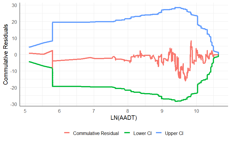
(a) AADT

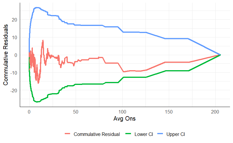
(b) Avg On

Fig. 7.: CURE plots for RPNB-L model

5.3 Key contributing risk variables

As previously discussed, the integration of a mixed distribution and random parameterization enabled the RPNB-L model to significantly outperform both the traditional NB model and the NB-L model with fixed coefficients. The NB-L mixed distribution effectively addresses overdispersion, while including random parameters allows the model to capture location-specific variations across bus stops, accounting for heterogeneity that fixed-coefficient models may overlook. This section examines the key factors identified by the RPNB-L model as contributing to pedestrian crash frequency nearbus stop locations. To provide deeper insights into the impact of these factors, average marginal effects were calculated for the significant variables. These marginal effects quantify the extent to which changes in each explanatory variable influence the expected number of crashes, offering a clear understanding of the real-world implications of these variables. The methodology for calculating marginal effects is detailed in section 4.4, and the results are presented in Table 4. This table highlights the variables with the most significant impact on crash frequency, providing valuable guidance for safety improvements and targeted interventions. Understanding these effects allows policymakers and transportation agencies to prioritize efforts aimed at reducing crashes at bus stops, especially in high-risk areas.

Table 4: RPNB-L based average marginal effects of crash contributing variables

Risk factors	Effects (Mean)
Ln (AADT)	0.259
Avg on	0.008
Int t (Ref. Non-signalized)	-0.247
Proximity (Ref. Near)	-0.188
School +1 (Ref. School 1 or 0)	0.417
Speed limit 35 mph (Ref. Speed limit¿35)	0.336
Med t (Ref. Divided)	0.245
Area Mix (Ref. Com and Res)	-0.275
Lighting (Ref. Yes)	0.075
Marked Xwalk (Ref. Yes)	0.074
Sidewalk (Ref. No)	-0.284

5.3.1 Vehicular traffic

The results, presented in Table 4, indicate that vehicular traffic, represented by Ln(AADT), has a significant influence on pedestrian crash frequency near bus stops. The RPNB-L model confirms that Ln(AADT) is statistically significant at the 95% credible interval, with a positive association between traffic volume and crash frequency. Specifically, the estimated mean coefficient for Ln(AADT) is 0.345, suggesting that an increase in traffic volume corresponds to a higher likelihood of pedestrian crashes at bus stops. This finding aligns with the intuitive expectation that greater vehicular flow increases pedestrian exposure to potential conflicts, thereby elevating crash risks. These results are consistent with previous studies that highlight the dangers of high traffic volumes near bus stops. Bus stops are often located in high-density passenger areas, where commuting involves significant traffic movement, increasing pedestrian exposure and risk (Tiboni and Rossetti, 2013). The absence of dedicated bus lanes further compounds this issue, as buses operating in mixed traffic environments negatively affect pedestrian safety (Yendra et al., 2024). Studies have also established that higher AADT levels are associated with increased pedestrian fatalities in such environments (Ulak et al., 2021; Lakhotia et al., 2020; Hess et al., 2004; Amadori and Bonino, 2012). Moreover, the model incorporates random parameterization for LnAADT, with a standard deviation of 0.042, which highlights the variability in the impact of traffic volume across different bus stop locations. This suggests that while traffic volume generally increases crash frequency, the magnitude of this effect can differ from one site to another. Some bus stops may experience a steeper increase in crash risk with rising traffic volumes, whereas others may be less affected. This variability underscores the importance of considering site-specific factors when evaluating the impact of vehicular traffic on pedestrian safety at bus stops.

5.3.2 Passengers density

In this study, pedestrian density near bus stops was represented by the mean number of passengers boarding and alighting at each stop, given the challenges of capturing real-time density. The model results indicate that higher pedestrian exposure, as reflected in increased boarding activity, is positively associated with a higher frequency of crashes. Greater pedestrian volumes increase the likelihood of vehicle-pedestrian interactions, leading to elevated crash risks. The estimated mean coefficient for the ”Avg on” variable is 0.010, with a standard deviation of 0.008, indicating that as pedestrian exposure rises, so does the risk of crashes. However, the effect varies across different bus stops, influenced by factors such as traffic conditions and surrounding infrastructure. These findings align with prior research (Hess et al., 2004; Geedipally, 2021; Craig et al., 2019), which consistently links high pedestrian volumes near bus stops to elevated crash risks, particularly in dense areas such as schools or commercial zones, where large groups of pedestrians frequently gather. Both the model and previous studies emphasize that increased pedestrian density raises exposure to traffic, thereby increasing the risk of crashes. These results underscore the importance of targeted safety measures and infrastructure improvements at high-volume bus stops.

Vehicle Speed The results of this study reveal a paradox: lower speed limits (35 mph or less) near bus stops are associated with an increase in pedestrian crashes. One potential reason is that pedestrians may feel safer with lower speed limits, leading them to cross the road more frequently and increasing their exposure to potential collisions. Additionally, despite the reduced speed limits, some drivers may still exceed the limit, resulting in unpredictable driving behaviors that further elevate crash risks. Previous research has primarily focused on the dangers of high-traffic speeds near bus stops. Studies have consistently linked higher speeds to an increased likelihood of pedestrian fatalities (Rossetti et al., 2020; Pulugurtha and Vanapalli, 2008; Hess et al., 2004; Lakhotia et al., 2020). Consequently, researchers have often recommended lower speed limits to enhance pedestrian safety (Ulak et al., 2021; Tubis et al., 2021; Pessaro et al., 2017). However, the findings from this study suggest that simply reducing speed limits may not be enough to mitigate crash risks. To effectively improve safety, stricter speed enforcement and enhanced pedestrian infrastructure such as crosswalks, pedestrian signals, and traffic calming measures are necessary. These measures can help ensure that drivers comply with speed limits while providing pedestrians with safe crossing options, thereby reducing the risk of vehicle-pedestrian conflicts near bus stops.

5.3.3 Nearest intersection

The findings of this study indicate that signalized intersections near bus stops are associated with a lower likelihood of pedestrian crashes compared to non-signalized intersections, as reflected by the negative coefficient (-0.329). This suggests that traffic signals enhance the management of pedestrian and vehicle movements, reducing potential conflicts and improving safety outcomes. In contrast, previous research has generally found that bus stops near intersections, whether signalized or not, pose greater risks for pedestrians due to higher traffic volumes and complex turning movements (Geedipally, 2021; Quistberg et al., 2015b). However, Samani and Amador-Jimenez (2023) reported that stop signs at non-signalized intersections can enhance safety by slowing down vehicles and structuring traffic more effectively. The difference between this study’s findings and previous research may stem from signalized intersections’ ability to regulate traffic flow and pedestrian behavior better. This highlights the importance of enhancing traffic control measures at non-signalized intersections to further improve pedestrian safety near bus stops. Strengthening such controls can reduce crash risks by ensuring more predictable interactions between pedestrians and vehicles, particularly in high-traffic areas.

5.3.4 Bus stops proximity

The proximity of bus stops to intersections plays a critical role in pedestrian crash risks. In this study, bus stops are categorized into three types based on their location: far-side, near-side, and mid-block. Far-side stops are located after intersections, near-side stops are positioned before intersections, and mid-block stops are situated between intersections. The model results indicate that far-side bus stops are associated with a significantly lower likelihood of pedestrian crashes compared to both near-side and mid-block stops, aligning with previous research (Fitzpatrick and Nowlin, 1997; Yu, 2024). Far-side stops are considered safer because they reduce pedestrian-vehicle conflicts by allowing pedestrians to cross with greater visibility and ensuring that they cross behind the bus or at the nearest marked crosswalk. In contrast, near-side stops are associated with higher crash risks, likely due to reduced driver visibility and the tendency for pedestrians to cross in front of the bus, where drivers may not anticipate their movements. Similarly, mid-block stops pose increased risks because they often lack proper pedestrian infrastructure, such as marked crosswalks, leading to unpredictable crossing behavior (Truong and Somenahalli, 2011; Pessaro et al., 2017; Rossetti et al., 2020).

5.3.5 Median types

The findings of this study show that the absence of medians on roadways near bus stops significantly increases the likelihood of pedestrian crashes compared to streets equipped with medians. Medians serve as pedestrian refuges, allowing individuals to cross the road in stages and reducing their exposure to traffic. In contrast, undivided roadways require pedestrians to cross the entire width of the road at once, which increases crash risk due to unpredictable crossing behavior and reduced driver visibility. These results align with previous studies that highlight the safety benefits of medians in reducing pedestrian-vehicle conflicts by providing protected spaces for pedestrians to pause mid-crossing (Yu, 2024; Salum et al., 2024; Jeng et al., 2003). Medians offer an essential safety buffer, particularly on wide or high-traffic roads, helping to reduce crash risks by giving pedestrians more predictable crossing points. The study’s findings reinforce the importance of incorporating medians as a key element in road design near bus stops to enhance pedestrian safety. Strategically placed medians ensure safer pedestrian movement and minimize potential conflicts with vehicles, ultimately contributing to reduced crash risks (Pessaro et al., 2017).

5.3.6 Lighting

The model results indicate that inadequate lighting near bus stops significantly increases the likelihood of pedestrian crashes, as reflected by the positive coefficient of 0.100 in the RPNB-L model. Poorly lit bus stops pose a higher risk because reduced visibility makes it difficult for both pedestrians and drivers to anticipate movements, particularly during nighttime hours. These findings are consistent with previous research emphasizing the importance of adequate lighting in enhancing safety at bus stops. Mukherjee et al. (2023) identified a direct relationship between insufficient lighting and higher pedestrian fatalities, especially in areas with sparse land use. Similarly, Tiboni and Rossetti (2013) found that 8% of the surveyed bus stops lacked artificial lighting, contributing to unsafe conditions.Moreover, studies consistently recommend enhanced illumination at bus stops and along their approaches to reduce crash risks (Pessaro et al., 2017; Salum et al., 2024). Adequate lighting ensures that both drivers and pedestrians have clear visibility, enabling them to anticipate movements and react appropriately, thereby lowering crash frequency. Overall, both the model results and supporting literature strongly indicate that improving lighting around bus stops is a critical safety measure to mitigate pedestrian crash risks.

5.3.7 Marked crosswalk

The model results indicate that the absence of marked crosswalks near bus stops is associated with a higher risk of pedestrian crashes, as reflected by the positive coefficient of 0.074. This finding suggests that locations without marked crosswalks are more likely to experience pedestrian crashes. Marked crosswalks provide a designated space for pedestrians to cross safely, reducing their exposure to traffic and improving the predictability of pedestrian movements for drivers. Without marked crosswalks, pedestrians are more likely to cross at unpredictable locations, increasing the risk of crashes due to reduced driver awareness and slower response times. The presence of crosswalks also helps organize traffic flow by signaling drivers to anticipate pedestrian activity, leading to safer road interactions. These findings align with previous research highlighting the importance of marked pedestrian crossings for improving safety around bus stops. For instance, Tiboni and Rossetti (2013) found that over 30% of inspected bus stops lacked marked crossings, contributing to unsafe conditions for pedestrians. Similarly, Mukherjee et al. (2023) demonstrated that the presence of zebra markings at pedestrian crossings can reduce the likelihood of fatal crashes by 23%, particularly during nighttime, by enhancing driver awareness of potential pedestrian interactions.The literature further emphasizes the value of pedestrian traffic signals in conjunction with crosswalks to enhance safety. Studies show that pedestrian signals help regulate both driver and pedestrian behavior, encouraging drivers to expect pedestrians in crosswalks and prompting pedestrians to use the designated areas safely (Jeng et al., 2003; Samani and Amador-Jimenez, 2023). In the absence of such infrastructure, pedestrians are more likely to take risks, especially on wider roadways or at bus stops without proper crossing facilities (Lakhotia et al., 2020).

5.3.8 Sidewalks

The model results from Tables 3 and 4 show that the absence of sidewalks near bus stops significantly increases the likelihood of pedestrian crashes, as reflected by the negative coefficient of -0.379. This finding suggests that without sidewalks, pedestrians are more exposed to traffic, often forced to walk on the road, which increases the risk of vehicle-pedestrian collisions. Sidewalks provide a designated space for pedestrians, minimizing their interaction with traffic and reducing crash risks. These results are consistent with previous research that emphasizes the critical role of sidewalks in enhancing pedestrian safety near bus stops. Pessaro et al. (2017) highlighted that proper pedestrian infrastructure, such as sidewalks, encourages safer walking behavior and signals to pedestrians that they are welcome in the environment. Similarly, Sukor and Fisal (2020) found that safety is the strongest factor influencing walkability to bus stops, further reinforcing the importance of adequate sidewalks. Tiboni and Rossetti (2013) discovered that one-third of the bus stops they surveyed lacked sidewalks, which exposed pedestrians to greater traffic risks. Likewise, Rossetti and Tiboni (2020) emphasized that pedestrians who walk along roadways without sidewalks face an increased risk of crashes. Overall, it highlights that the presence of sidewalks is crucial for reducing pedestrian-vehicle interactions and ensuring safer access to bus stops (Yu, 2024; Samani and Amador-Jimenez, 2023; Lakhotia et al., 2020; Mukherjee et al., 2023), making it a critical element of pedestrian infrastructure.

5.3.9 Schools

TThe findings of this study, supported by existing literature, demonstrate that the presence of schools near bus stops significantly increases the likelihood of pedestrian crashes. The model results indicate that higher pedestrian density around schools, especially during peak times, leads to more pedestrian-vehicle interactions, thereby elevating the risk of crashes. While many students may be dropped off directly at school by buses, the presence of schools increases pedestrian activity around nearby bus stops, which raises the potential for conflicts between pedestrians and vehicles. These findings align with previous research. Craig et al. (2019) and Geedipally (2021) found that bus stops near schools are associated with a higher incidence of collisions due to the concentration of pedestrians. Similarly, Hess et al. (2004) noted that the gathering of students around bus stops often leads to unpredictable pedestrian behavior, further heightening the risk of crashes.

5.3.10 Area use

Previous research has identified bus stops in high pedestrian activity areas, particularly in commercial zones with heavy traffic, as high-risk locations for pedestrian crashes. These elevated risks are often attributed to poor integration with surrounding land use and proximity to parking areas, which create additional conflict points between pedestrians and vehicles (Pessaro et al., 2017; Hess et al., 2004). However, the findings of this study suggest that bus stops located in mixed-use areas—which combine residential, commercial, and recreational spaces—exhibit a lower likelihood of pedestrian crashes compared to those in strictly commercial or residential zones. This reduction in crash risk may be attributed to balanced traffic flows and the presence of improved infrastructure, such as sidewalks, crosswalks, proper lighting, and warning signs. In addition, enhanced safety measures like speed bumps and pedestrian signals in mixed-use areas further contribute to safer environments. Drivers in these zones may also exercise greater caution, given the diverse types of road users, including residents and recreational pedestrians.

5.4 KABC and KAB crashes

The estimated RPNB-L models for KABC and KAB pedestrian crashes reveal several important insights when compared with the total pedestrian crash model (KABCO), as presented in Table 5. First, most of the significant risk factors identified in the KABCO model remain consistent across the KABC and KAB models. However, an exception was observed with the marked crosswalk and sidewalk variables, which did not achieve statistical significance at the 95% confidence level in the KAB models. This suggests that these features may exert a greater influence on less severe crashes, primarily reflected in the KABCO and KABC models. Second, similar to the KABCO model, traffic volume and average passenger boarding were found to be randomly distributed across locations in both the KABC and KAB models. For the KABC model, the coefficient of the average volume mean is 0.355 with a standard deviation of 0.0048. In contrast, the impact of average volume in the KAB model is reduced, with a mean value of 0.191 and a standard deviation of 0.313. A similar trend was observed for the average boarding passengers parameter coefficient, indicating that the relationship between traffic volume, speed limits, and pedestrian crash severity varies between severe (KAB) and non-severe (KABC) crashes. Specifically, higher traffic volumes and lower speed limits are more often associated with non-severe crashes, while lower traffic volumes on higher-speed roads tend to result in more severe crashes. The posterior parameter estimates further reveal that bus stops near signalized intersections experience significantly fewer KABC and KAB crashes compared to those near non-signalized intersections. This finding emphasizes the importance of signalized intersections in reducing pedestrian crash risks, particularly for more severe incidents.

Table 5: Model Estimation Results for KABC and KAB crashes

Variable	KABC crashes			KAB crashes
		95% CI			95% CI
	$\beta$ (Std. Dev.)	LL	UL	$\beta$ (Std. Dev.)	LL	UL
Parameter mean
(Intercept)	-0.491 (0.035)	-0.654	-0.301	-0.453 (0.027)	-0.643	-0.227
Ln (AADT)	0.355 (0.081)	0.090	0.421	0.191 (0.063)	0.025	0.441
Avg on	0.010(0.004)	0.001	0.012	0.007 (0.001)	0.001	0.009
Int t (Ref. Non-signalized)	-0.339(0.110)	-0.665	-0.016	-0.292 (0.098)	-0.372	-0.045
Proximity (Ref. Near)	-0.253(0.140)	-0.521	-0.0271	-0.312 (0.167)	-0.656	-0.061
School (Ref. School 1)	0.559(0.179)	0.199	0.907	0.641 (0.187)	0.210	1.108
Speed limit (Ref. Speed limit¿35)	0.454(0.166)	0.133	0.771	0.393 (0.108)	0.087	0.661
Med t (Ref. Divided)	0.331(0.151)	0.0489	0.647	0.217 (0.089)	0.035	0.446
Area Mix (Ref. Com and Res)	-0.361(0.163)	-0.767	-0.048	-0.415(0.186)	-0.917	-0.029
Lighting (Ref. Yes)	0.110(0.090)	0.024	0.217	0.231 (0.089)	0.054	0.412
Marked Xwalk (Ref. Yes)	0.096 (0.074)	0.005	0.396
Sidewalk (Ref. No)	-0.382(0.189)	-0.667	-0.221
Dispersion parameter ($\alpha$)	0.147(0.081)	0.059	0.385	0.214(0.118)	0.119	0.692
Lindley parameter ($\theta$)	1.417(0.166)	1.267	1.786	1.419(0.168)	1.244	1.778
Std. Dev. of Random Parameters
Ln (AADT)	0.048 (0.003)	0.044	0.051	0.313 (0.154)	0.078	0.546
Avg on	0.008 (0.001)	0.003	0.010	0.043 (0.022)	0.010	0.132
Performance measure
DIC		1187.1			869.56
Dbar		997.8			765.06
Pd		189.3			131.5
MAE (Train)		0.677			0.449
MAE (Test)		0.768			0.505
RMSE (Train)		0.876			0.577
RMSE (Test)		0.982			0.676

5.5 Hazard bus stops identification

The identification of hazardous bus stops, defined as locations with a higher expected number of crashes compared to similar stops (Elvik 2007), is crucial for authorities (Hauer and Persaud, 1984; Persaud et al., 1999; Miranda-Moreno et al., 2007; Montella, 2010). These high-risk locations are often the starting point for decisions on where to invest in remedial safety actions. A common approach to hotspot identification involves generating an ordered list of sites ranked from highest to lowest risk (Hauer et al., 2002; Hauer, 2004). However, this task is challenging due to inherent randomness, yearly fluctuations in crash data at individual locations, and the regression-to-the-mean (RTM) bias (Hauer and Persaud, 1984). The RTM bias reflects the tendency for extreme crash frequencies at a given location to revert toward the long-term average over time due to random variation. Failure to account for RTM may result in misidentifying sites as high-risk based on short-term crash spikes or overlooking hazardous locations during periods of unusually low crash occurrence, leading to suboptimal allocation of safety interventions. This bias can be overcome identifying hotspots based on expected crash frequencies (Hauer, 1997), which can be calculated through Full bayes (FB) and empirical bayes (EB) methods (Miranda-Moreno et al., 2007; Montella, 2010; Khodadadi et al., 2022). The FB method leverages the hierarchical structure of Bayesian models to generate random samples from the posterior distribution without needing a closed-form solution. This flexibility allows it to handle complex models more effectively than traditional methods, enabling more accurate parameter estimation and predictions. This study adopted the Full Bayes (FB) method to estimate expected crash frequencies and determined hotspots applying Potential for Safety Improvement (PSI) approach, it calculates the difference between expected and predicted crashes (Hauer et al., 2002). The expected crash frquency at each stops can be calculated following Eqn 25, and for a deeper understanding, readers are directed to Khodadadi et al., 2022.

$$p(y_{\text{exp}}\mid y_{\text{obs}})=\int_{\eta,\phi}NB\left(e^{-\eta},\phi\right)\left(\int_{b}p(\eta\mid b,y_{\text{obs}})\,\pi_{b}\,db\right)\,\pi_{\phi}\,d\eta\,d\phi$$ (25)

Based on PSI scores, bus stops can be classified into three categories: PSI is positive, and stops in the top 10% are classified as hotspots, indicating a high potential for safety improvements, while those with positive PSI values not in the top 10% are classified as normal zones, which still require attention but are less critical. Cold zones have negative PSI values, indicating that they are relatively safer, as shown in Fig.5.5(a). This method identifies hazardous bus stops and allows for a detailed understanding of the corridors (see: Fig.5.5b). Once the hazardous corridors are identified, transportation agencies can prioritize their interventions, specially when they have low budgets.

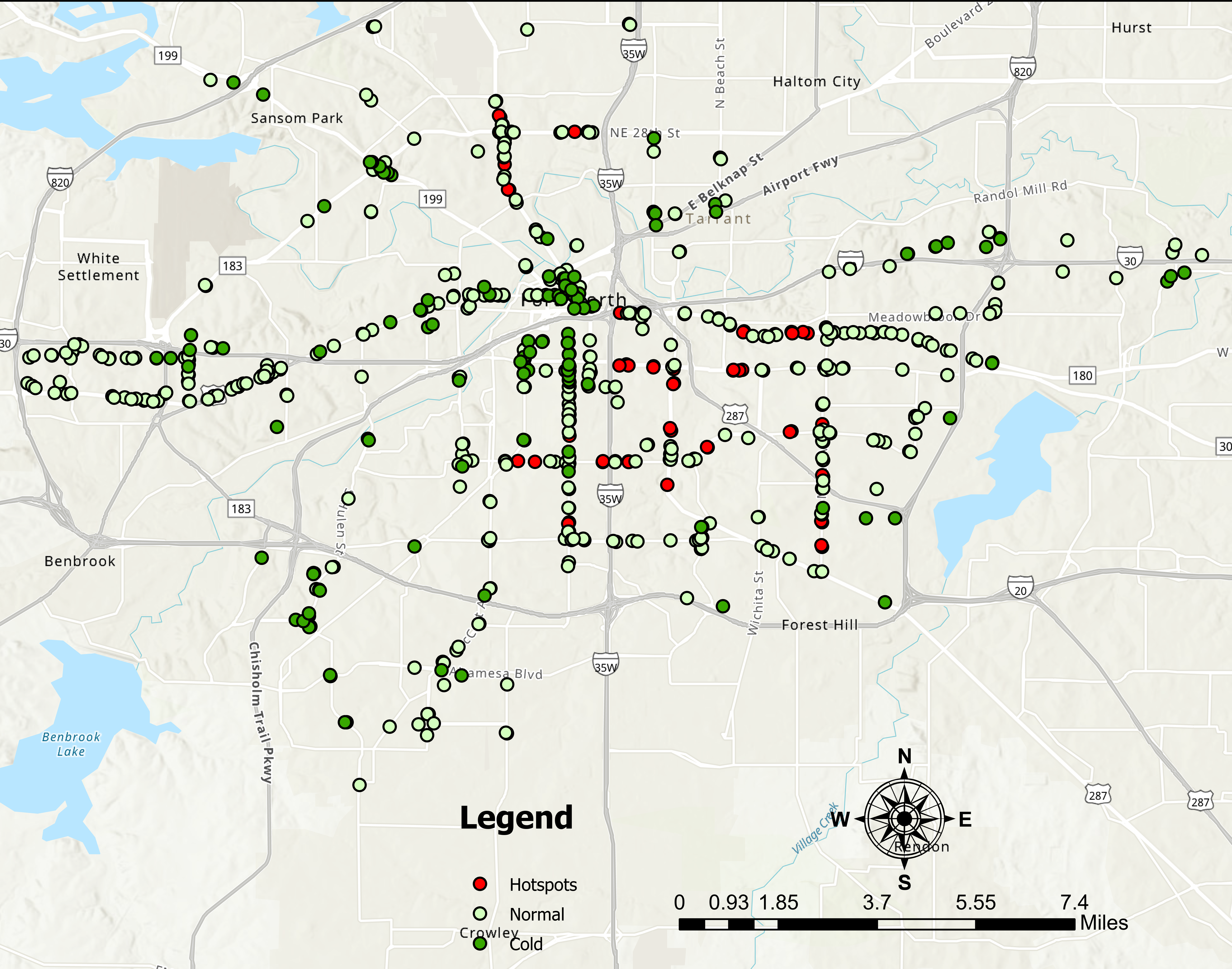
(a) Bus stops catagories

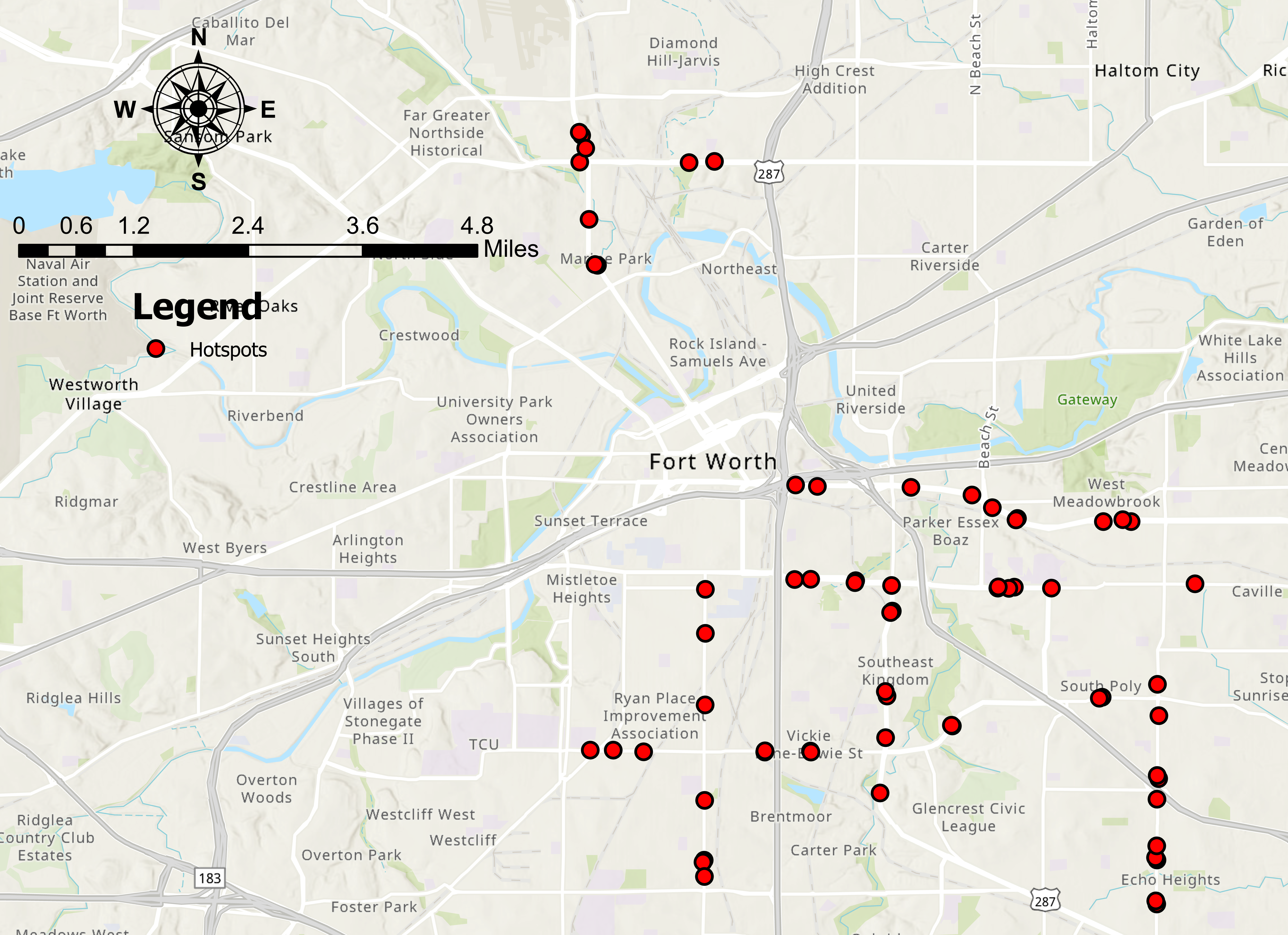
(b) Hotspots

Fig. 8.: Hazard bus stops corridor identification

6 Summary and Conclusions

This study addresses the critical issue of pedestrian safety near bus stops, emphasizing the need to understand the factors influencing crashes in these environments. Despite the essential role of bus stops in urban transportation, limited research exists on safety concerns specific to these locations. The lack of targeted interventions stems from inadequate knowledge of crash-contributing factors, hindering the development of effective countermeasures. To bridge this gap, the study employed advanced statistical models to develop Safety Performance Functions (SPFs), exploring the relationship between various traffic, roadway environment, and bus stop design-related factors and pedestrian crash occurrences. By identifying hazardous bus stop locations or hotspots, the study aims to guide transportation agencies in implementing targeted safety interventions and enhancing urban transportation systems’ overall reliability and safety.

The study analyzed pedestrian crash data from 2018 to 2022 across 596 bus stops in Fort Worth, Texas, integrating roadway attributes, geometric features, and operational data. The high proportion of zero-crash sites and right-skewed distribution of the crash data necessitated the use of advanced models. The Random Parameters Negative Binomial-Lindley (RPNB-L) model demonstrated superior performance over traditional Negative Binomial (NB) and NB-L models, as it captured unobserved heterogeneity and variability across bus stops. The RPNB-L model’s ability to account for location-specific characteristics made it more accurate in predicting crash risks.

The results of the proposed RPNB-L model identified several key factors significantly influencing pedestrian crash. The analysis revealed that variables such as AADT, average boarding passengers, intersection types, proximity to intersections, median types, school counts, speed limits, area types, sidewalk presence, lighting, and marked crosswalks are critical contributors to pedestrian crashes. The model also demonstrated its capacity to capture spatial relationships between traffic attributes, such as traffic volume and passenger boarding patterns, further enhancing its predictive power.

In terms of geometric features, the results indicate that bus stops near signalized intersections showed a reduced likelihood of crashes, indicating the positive impact of controlled crossings. Conversely, bus stops near non-signalized intersections and near-side stops were associated with higher crash frequencies. Stops with medians provided safer crossing opportunities, underscoring their importance in bus stop design to mitigate pedestrian risks. The analysis revealed a counterintuitive relationship between speed limits and crash risk. While lower speed limits (35 mph or below) are typically intended to improve safety, the study found that such zones experienced more crashes, possibly due to increased pedestrian activity and a false sense of security among pedestrians. Additionally, high pedestrian density around bus stops located near schools increased the frequency of crashes, driven by the greater volume of pedestrian movements during peak hours. In contrast, mixed-use areas exhibited lower crash rates, likely due to balanced traffic flow, better infrastructure, and heightened driver awareness.

Infrastructure features such as sidewalks, crosswalks, and lighting played a significant role in reducing pedestrian crash risks. Adequate lighting was particularly effective in preventing crashes during low-visibility conditions, such as at night or in inclement weather. The absence of marked crosswalks increased the likelihood of crashes, highlighting the importance of well-defined pedestrian crossings. Similarly, the presence of sidewalks reduced pedestrian exposure to vehicular traffic, lowering crash risks. The study identified several high-risk bus stops and corridors concentrated in transition areas, where changes in road design, speed limits, or land use occur. These sections require targeted interventions and continuous monitoring to mitigate potential safety risks. Using the Full Bayes (FB) method, the study applied the Potential for Safety Improvement (PSI) metric to estimate expected crash frequencies and prioritize hazardous locations for intervention.

The findings offer valuable insights for transportation agencies, guiding efforts to enhance pedestrian safety through a combination of infrastructure improvements, signage upgrades, speed control measures, and public education campaigns. Special attention should be given to non-signalized intersections, high-traffic areas, and locations with increased pedestrian activity, such as near schools. While the study provides essential insights, it is important to acknowledge its limitations. First, the findings are based on data from Fort Worth, Texas, which may limit their generalizability to other regions. Second, the study relies on historical crash data, which may contain inaccuracies, underreporting, or missing information (Arun et al., 2021). The inability to directly observe pedestrian behavior or capture real-time exposure (such as passenger boarding or alighting patterns) may affect the accuracy of the models. While advanced statistical techniques address unobserved heterogeneity, bias from omitted variables or measurement errors cannot be fully eliminated. The study also focuses primarily on crashes at bus stops without considering the entire pedestrian journey, which could overlook risks along those routes. Additionally, factors such as weather conditions, enforcement levels, and cultural attitudes toward pedestrian safety were not included in the models. Finally, the study does not address the specific safety needs of vulnerable groups such as children, the elderly, and individuals with disabilities, who may exhibit different behaviors and risks.

Future research should focus on expanding the geographic scope of the models to other urban areas, developing adjustment factors to improve transferability, and analyzing different types of crashes (e.g., fatal versus non-fatal) to enhance predictive accuracy. Real-time pedestrian exposure data, such as GPS tracking or pedestrian surveys, could provide a more dynamic understanding of behavior and risk. Research should also prioritize vulnerable populations, examining the unique risks faced by children, the elderly, and individuals with disabilities, who rely heavily on public transportation. Further investigation into pedestrian safety in low-density areas, where data are scarce and challenges such as street vendor encroachment are common, could also provide valuable insights. Surrogate safety measures, such as traffic conflicts (Li et al., 2024; Anis et al., 2024), offer a promising alternative to crash data in resource-constrained settings and should be explored in future studies.

This study emphasizes the importance of understanding the dynamics of pedestrian safety at bus stops to develop effective, data-driven interventions. The RPNB-L model proved to be a robust tool for identifying key crash predictors and hazardous locations, offering a framework for enhancing pedestrian safety. By addressing critical infrastructure needs and promoting safety-focused policies, transportation agencies can reduce crash risks and encourage safer public transportation usage in urban areas.

Acknowledgement:

The authors express their sincere gratitude to TxDOT for sponsoring the project from which this paper is derived. The authors thank TxDOT and Trinity Metro for providing the crash and bus stop data required for this paper.

Disclaimer:

The results presented in this document do not necessarily reflect those from the TxDOT.

Data availability:

Data and code will be made available on reasonable request.

References

- Akintayo and Adibeli 2022 Akintayo, F.O., Adibeli, S.A., 2022. Safety performance of selected bus stops in ibadan metropolis, nigeria. Journal of Public Transportation 24, 100003.
- Amadori and Bonino 2012 Amadori, M., Bonino, T., 2012. A methodology to define the level of safety of public transport bus stops, based on the concept of risk. Procedia-Social and Behavioral Sciences 48, 653–662.
- Anastasopoulos and Mannering 2009 Anastasopoulos, P.C., Mannering, F.L., 2009. A note on modeling vehicle accident frequencies with random-parameters count models. Accident Analysis & Prevention 41, 153–159.
- Anis et al. 2024 Anis, M., Li, S., Geedipally, S.R., Zhou, Y., Lord, D., 2024. Real-time risk estimation for active road safety: Leveraging waymo av sensor data with hierarchical bayesian extreme value models. arXiv preprint arXiv:2407.16832 .
- Arun et al. 2021 Arun, A., Haque, M.M., Bhaskar, A., Washington, S., Sayed, T., 2021. A systematic mapping review of surrogate safety assessment using traffic conflict techniques. Accident Analysis & Prevention 153, 106016.
- Barua et al. 2016 Barua, S., El-Basyouny, K., Islam, M.T., 2016. Multivariate random parameters collision count data models with spatial heterogeneity. Analytic methods in accident research 9, 1–15.
- Beck et al. 2007 Beck, L.F., Dellinger, A.M., O’neil, M.E., 2007. Motor vehicle crash injury rates by mode of travel, united states: using exposure-based methods to quantify differences. American Journal of Epidemiology 166, 212–218.
- Campbell et al. 2003 Campbell, B.J., Zegeer, C.V., Huang, H.H., Cynecki, M.J., et al., 2003. A review of pedestrian safety research in the united states and abroad .
- Chand and Chandra 2017 Chand, S., Chandra, S., 2017. Improper stopping of buses at curbside bus stops: Reasons and implications. Transportation in developing economies 3, 1–9.
- Clifton et al. 2009 Clifton, K.J., Burnier, C.V., Akar, G., 2009. Severity of injury resulting from pedestrian–vehicle crashes: What can we learn from examining the built environment? Transportation research part D: transport and environment 14, 425–436.
- Clifton and Kreamer-Fults 2007 Clifton, K.J., Kreamer-Fults, K., 2007. An examination of the environmental attributes associated with pedestrian–vehicular crashes near public schools. Accident Analysis & Prevention 39, 708–715.
- Craig et al. 2019 Craig, C.M., Morris, N.L., Van Houten, R., Mayou, D., 2019. Pedestrian safety and driver yielding near public transit stops. Transportation research record 2673, 514–523.
- Das et al. 2019 Das, S., Dutta, A., Avelar, R., Dixon, K., Sun, X., Jalayer, M., 2019. Supervised association rules mining on pedestrian crashes in urban areas: identifying patterns for appropriate countermeasures. International Journal of Urban Sciences 23, 30–48.
- El-Basyouny and Sayed 2009 El-Basyouny, K., Sayed, T., 2009. Urban arterial accident prediction models with spatial effects. Transportation research record 2102, 27–33.
- Elvik 2007 Elvik, R., 2007. State-of-the-art approaches to road accident black spot management and safety analysis of road networks. Transportøkonomisk institutt Oslo, Norway.
- Fitzpatrick and Nowlin 1997 Fitzpatrick, K., Nowlin, R.L., 1997. Effects of bus stop design on suburban arterial operations. Transportation Research Record 1571, 31–41.
- Geedipally 2021 Geedipally, S., 2021. Effects of bus stops on pedestrian safety at signalized intersections, in: Conference of Transportation Research Group of India, Springer. pp. 131–144.
- Geedipally et al. 2012 Geedipally, S.R., Lord, D., Dhavala, S.S., 2012. The negative binomial-lindley generalized linear model: Characteristics and application using crash data. Accident Analysis & Prevention 45, 258–265.
- Gelfand et al. 1995 Gelfand, A.E., Sahu, S.K., Carlin, B.P., 1995. Efficient parametrisations for normal linear mixed models. Biometrika 82, 479–488.
- Gelman and Rubin 1992 Gelman, A., Rubin, D.B., 1992. Inference from iterative simulation using multiple sequences. Statistical science 7, 457–472.
- Haleem et al. 2015 Haleem, K., Alluri, P., Gan, A., 2015. Analyzing pedestrian crash injury severity at signalized and non-signalized locations. Accident Analysis & Prevention 81, 14–23.
- Harwood et al. 2008 Harwood, D.W., Bauer, K.M., Richard, K.R., Gilmore, D.K., Graham, J.L., Potts, I.B., Torbic, D.J., Hauer, E., 2008. Pedestrian safety prediction methodology. Technical Report.
- Hauer 1997 Hauer, E., 1997. Observational before/after studies in road safety. Estimating the effect of highway and traffic engineering measures on road safety.
- Hauer 2004 Hauer, E., 2004. Statistical road safety modeling. Transportation Research Record 1897, 81–87.
- Hauer et al. 2002 Hauer, E., Kononov, J., Allery, B., Griffith, M.S., 2002. Screening the road network for sites with promise. Transportation Research Record 1784, 27–32.
- Hauer and Persaud 1984 Hauer, E., Persaud, B.N., 1984. Problem of identifying hazardous locations using accident data. Transportation Research Record 975, 36–43.
- Hess et al. 2004 Hess, P.M., Moudon, A.V., Matlick, J.M., 2004. Pedestrian safety and transit corridors. Journal of Public Transportation 7, 73–93.
- on Development of the Highway Safety Manual and on the Highway Safety Manual 2010 on Development of the Highway Safety Manual, N.R.C.U.T.R.B.T.F., on the Highway Safety Manual, T.O.J.T.F., 2010. Highway safety manual. volume 1. AASHTO.
- Hu and Cicchino 2018 Hu, W., Cicchino, J.B., 2018. An examination of the increases in pedestrian motor-vehicle crash fatalities during 2009–2016. Journal of safety research 67, 37–44.
- Institute and Foundation 1996 Institute, T.T., Foundation, T.A..M.R., 1996. Guidelines for the location and design of bus stops. volume 19. National Academy Press.
- Jeng et al. 2003 Jeng, O.J., Fallat, G., et al., 2003. Pedestrian Safety and Mobility Aids for Crossings at Bus Stops. Technical Report. New Jersey. Department of Transportation. Bureau of Research.
- Khodadadi et al. 2023 Khodadadi, A., Shirazi, M., Geedipally, S., Lord, D., 2023. Evaluating alternative variations of negative binomial–lindley distribution for modelling crash data. Transportmetrica A: transport science 19, 2062480.
- Khodadadi et al. 2022 Khodadadi, A., Tsapakis, I., Shirazi, M., Das, S., Lord, D., 2022. Derivation of the empirical bayesian method for the negative binomial-lindley generalized linear model with application in traffic safety. Accident Analysis & Prevention 170, 106638.
- Kuşkapan et al. 2022 Kuşkapan, E., Sahraei, M.A., Çodur, M.K., Çodur, M.Y., 2022. Pedestrian safety at signalized intersections: Spatial and machine learning approaches. Journal of Transport & Health 24, 101322.
- Lakhotia et al. 2020 Lakhotia, S., Lassarre, S., Rao, K.R., Tiwari, G., 2020. Pedestrian accessibility and safety around bus stops in delhi. IATSS research 44, 55–66.
- Lee et al. 2015 Lee, J., Abdel-Aty, M., Choi, K., Huang, H., 2015. Multi-level hot zone identification for pedestrian safety. Accident Analysis & Prevention 76, 64–73.
- Li et al. 2017 Li, D., Ranjitkar, P., Zhao, Y., Yi, H., Rashidi, S., 2017. Analyzing pedestrian crash injury severity under different weather conditions. Traffic injury prevention 18, 427–430.
- Li et al. 2024 Li, S., Anis, M., Lord, D., Zhang, H., Zhou, Y., Ye, X., 2024. Beyond 1d and oversimplified kinematics: A generic analytical framework for surrogate safety measures. Accident Analysis & Prevention 204, 107649.
- Lord and Mannering 2010 Lord, D., Mannering, F., 2010. The statistical analysis of crash-frequency data: A review and assessment of methodological alternatives. Transportation research part A: policy and practice 44, 291–305.
- Lord and Miranda-Moreno 2008 Lord, D., Miranda-Moreno, L.F., 2008. Effects of low sample mean values and small sample size on the estimation of the fixed dispersion parameter of poisson-gamma models for modeling motor vehicle crashes: A bayesian perspective. Safety Science 46, 751–770.
- Lord et al. 2021 Lord, D., Qin, X., Geedipally, S.R., 2021. Highway safety analytics and modeling. Elsevier.
- Lord et al. 2005 Lord, D., Washington, S.P., Ivan, J.N., 2005. Poisson, poisson-gamma and zero-inflated regression models of motor vehicle crashes: balancing statistical fit and theory. Accident Analysis & Prevention 37, 35–46.
- Miranda-Moreno et al. 2007 Miranda-Moreno, L.F., Labbe, A., Fu, L., 2007. Bayesian multiple testing procedures for hotspot identification. Accident Analysis & Prevention 39, 1192–1201.
- Mitra and Washington 2007 Mitra, S., Washington, S., 2007. On the nature of over-dispersion in motor vehicle crash prediction models. Accident Analysis & Prevention 39, 459–468.
- Montella 2010 Montella, A., 2010. A comparative analysis of hotspot identification methods. Accident Analysis & Prevention 42, 571–581.
- Mukherjee et al. 2023 Mukherjee, D., Rao, K.R., Tiwari, G., 2023. Built-environment risk assessment for pedestrians near bus-stops: a case study in delhi. International journal of injury control and safety promotion 30, 185–194.
- Persaud et al. 1999 Persaud, B., Lyon, C., Nguyen, T., 1999. Empirical bayes procedure for ranking sites for safety investigation by potential for safety improvement. Transportation research record 1665, 7–12.
- Pessaro et al. 2017 Pessaro, B., Catalá, M., Wang, Z., Spicer, M., et al., 2017. Impact of transit stop location on pedestrian safety .
- Pulugurtha and Sambhara 2011 Pulugurtha, S.S., Sambhara, V.R., 2011. Pedestrian crash estimation models for signalized intersections. Accident Analysis & Prevention 43, 439–446.
- Pulugurtha and Vanapalli 2008 Pulugurtha, S.S., Vanapalli, V.K., 2008. Hazardous bus stops identification: An illustration using gis. Journal of Public Transportation 11, 65–83.
- Quistberg et al. 2015a Quistberg, D.A., Howard, E.J., Ebel, B.E., Moudon, A.V., Saelens, B.E., Hurvitz, P.M., Curtin, J.E., Rivara, F.P., 2015a. Multilevel models for evaluating the risk of pedestrian–motor vehicle collisions at intersections and mid-blocks. Accident Analysis & Prevention 84, 99–111.
- Quistberg et al. 2015b Quistberg, D.A., Koepsell, T.D., Johnston, B.D., Boyle, L.N., Miranda, J.J., Ebel, B.E., 2015b. Bus stops and pedestrian–motor vehicle collisions in lima, peru: a matched case–control study. Injury prevention 21, e15–e22.
- Rahman Shaon and Qin 2016 Rahman Shaon, M.R., Qin, X., 2016. Use of mixed distribution generalized linear models to quantify safety effects of rural roadway features. Transportation Research Record 2583, 134–141.
- Rossetti et al. 2020 Rossetti, S., Tiboni, M., et al., 2020. In field assessment of safety, security, comfort and accessibility of bus stops: A planning perspective. EUROPEAN TRANSPORT/TRASPORTI EUROPEI .
- Salum et al. 2024 Salum, J.H., Kisabanzira, N., Alluri, P., Sando, T., 2024. Toolkit for the assessment of safety at bus stops. Transportation research record 2678, 279–292.
- Samani and Amador-Jimenez 2023 Samani, R.R., Amador-Jimenez, L., 2023. Exploring road safety of pedestrians in proximity to public transit access points (bus stops and metro stations), a case study of montreal, canada. Canadian Journal of Civil Engineering 50, 536–547.
- Sanchez Rodriguez and Ferenchak 2024 Sanchez Rodriguez, O., Ferenchak, N.N., 2024. Longitudinal spatial trends in us pedestrian fatalities, 1999–2020. Transportation research record 2678, 904–916.
- Shaon et al. 2018 Shaon, M.R.R., Qin, X., Shirazi, M., Lord, D., Geedipally, S.R., 2018. Developing a random parameters negative binomial-lindley model to analyze highly over-dispersed crash count data. Analytic methods in accident research 18, 33–44.
- Shinar 2012 Shinar, D., 2012. Safety and mobility of vulnerable road users: pedestrians, bicyclists, and motorcyclists.
- Stewart 2023 Stewart, T., 2023. Overview of motor vehicle traffic crashes in 2021. Technical Report.
- Sukor and Fisal 2020 Sukor, N.S.A., Fisal, S.F.M., 2020. Safety, connectivity, and comfortability as improvement indicators of walkability to the bus stops in penang island. Engineering, Technology & Applied Science Research 10, 6450–6455.
- Thakali et al. 2015 Thakali, L., Kwon, T.J., Fu, L., 2015. Identification of crash hotspots using kernel density estimation and kriging methods: a comparison. Journal of Modern Transportation 23, 93–106.
- Tiboni and Rossetti 2013 Tiboni, M., Rossetti, S., 2013. Implementing a road safety review approach for existing bus stops. WIT Transactions on the Built Environment 130, 699–709.
- Toran Pour et al. 2017 Toran Pour, A., Moridpour, S., Tay, R., Rajabifard, A., 2017. Modelling pedestrian crash severity at mid-blocks. Transportmetrica A: Transport Science 13, 273–297.
- Torbic et al. 2010 Torbic, D.J., Harwood, D.W., Bokenkroger, C.D., Srinivasan, R., Carter, D., Zegeer, C.V., Lyon, C., 2010. Pedestrian safety prediction methodology for urban signalized intersections. Transportation research record 2198, 65–74.
- Truong and Somenahalli 2011 Truong, L.T., Somenahalli, S.V., 2011. Using gis to identify pedestrian-vehicle crash hot spots and unsafe bus stops. Journal of Public Transportation 14, 99–114.
- Tubis et al. 2021 Tubis, A.A., Skupień, E.T., Rydlewski, M., 2021. Method of assessing bus stops safety based on three groups of criteria. Sustainability 13, 8275.
- Tyndall 2021 Tyndall, J., 2021. Pedestrian deaths and large vehicles. Economics of Transportation 26, 100219.
- Ulak et al. 2021 Ulak, M.B., Kocatepe, A., Yazici, A., Ozguven, E.E., Kumar, A., 2021. A stop safety index to address pedestrian safety around bus stops. Safety Science 133, 105017.
- Walgren 1998 Walgren, S., 1998. Using geographic information system (gis) to analyze pedestrian accidents, in: 68th Annual Meeting of the Institute of Transportation EngineersInstitute of Transportation Engineers (ITE).
- Washington et al. 2020 Washington, S., Karlaftis, M.G., Mannering, F., Anastasopoulos, P., 2020. Statistical and econometric methods for transportation data analysis. Chapman and Hall/CRC.
- Wretstrand et al. 2014 Wretstrand, A., Holmberg, B., Berntman, M., 2014. Safety as a key performance indicator: Creating a safety culture for enhanced passenger safety, comfort, and accessibility. Research in transportation economics 48, 109–115.
- Xie et al. 2017 Xie, K., Ozbay, K., Kurkcu, A., Yang, H., 2017. Analysis of traffic crashes involving pedestrians using big data: Investigation of contributing factors and identification of hotspots. Risk analysis 37, 1459–1476.
- Yendra et al. 2024 Yendra, D., Haworth, N., Watson-Brown, N., 2024. A comparison of factors influencing the safety of pedestrians accessing bus stops in countries of differing income levels. Accident Analysis & Prevention 207, 107725.
- Yu 2024 Yu, C.Y., 2024. The impact of built environments on pedestrian safety around bus stops. Journal of Urban Affairs 46, 267–280.
- Zahabi et al. 2011 Zahabi, S.A.H., Strauss, J., Manaugh, K., Miranda-Moreno, L.F., 2011. Estimating potential effect of speed limits, built environment, and other factors on severity of pedestrian and cyclist injuries in crashes. Transportation research record 2247, 81–90.
- Zamani and Ismail 2010 Zamani, H., Ismail, N., 2010. Negative binomial-lindley distribution and its application. Journal of mathematics and statistics 6, 4–9.
- Zegeer and Bushell 2012 Zegeer, C.V., Bushell, M., 2012. Pedestrian crash trends and potential countermeasures from around the world. Accident Analysis & Prevention 44, 3–11.
- Zhang et al. 2023 Zhang, C., Du, B., Shen, J., Ma, C., 2023. Revealing safety impact of bus stops on passenger-cyclist interactions–evidence from nanjing, china. Travel behaviour and society 32, 100578.