Bloch classification surface for three-band systems

Abstract

Topologically protected states can be found in physical systems, that show singularities in some energy contour diagram. These singularities can be characterized by winding numbers, defined on a classification surface, which maps physical state parameters. We have found a classification surface, which applies for three-band hamiltonian systems in the same way than standard Bloch surface does for two-band ones. This generalized Bloch surface is universal in the sense that it classifies a very large class of three-band systems, which we have exhaustively studied, finding specific classification surfaces, applying for each one.

1 Introduction

In recent years, physicists have investigated new quantum states, such as zero-energy states like Majorana fermions[1, 2, 3], zero-mass particles associated to Dirac contact points[4, 5, 6] or anyons[7]. These quantum states are remarkable because they are protected by topological singularities.

Initiated by theoretical predictions[8, 9, 10, 11, 12, 1, 13, 14, 15], the quest of such topological states has spread into a larger and larger community of experimentalists and has provided more and more valid candidates[16, 17, 18, 19, 20, 21].

In most cases, these states are characterized by a quantum integer associated to some physical flux in real or reciprocal space. Following Gauss-Bonnet theorem[22, 23, 24], this quantum integer is also related to a path integral around a singularity. The choice of the integrand depends on which symmetry is relevant in each specific situation.

This approach proves to be very general: the classification of many topological states can be performed through that of closed paths, using the fundamental (also called first homotopy) group $\pi_{1}(\mathcal{E})$, which addresses winding numbers associated to specific symmetries of the system. Other topological systems need the second homotopy group $\pi_{2}(\mathcal{E})$, for which our results are not relevant. For the classification through $\pi_{1}(\mathcal{E})$ to be valid, it must be determined in an abstract space $\mathcal{E}$, where all states are represented faithfully.

In primitive theories[9, 15, 25], topological states are protected by energy gaps. However, more sophisticated cases may happen[14, 26] in three-band systems, where one gap closes. In such situations, using $\pi_{1}(\mathcal{E})$ to determinate winding numbers proves very efficient, while other means can fail.

$\mathcal{E}$ can be arbitrarily constructed by a bijective mapping of the states; however, for two-band systems, one can always choose Bloch surface, which is the standard $S_{2}$ sphere: it is universal in the sense that it can represent all two-band systems.

In three-band systems, one finds a very short list of surfaces, which can represent them. In particular, we have proved the existence of a generic surface $s_{6}$, which applies for almost all of them and can therefore be considered as the generalized Bloch surface of three-band systems. Its universality makes it a very powerful device, which can be used to study any $3\times 3$ matrix representation of a hamiltonian.

As we will explain, Bloch surface does not suffice to classify singular mappings: actually, one must not determinate $\pi_{1}(\mathcal{E})$ but $\pi_{1}(\mathcal{E}^{\prime})$ instead, where $\mathcal{E}^{\prime}$ is a specific subspace of $\mathcal{E}$, called effective surface, $\mathcal{E}^{\prime}\subset\mathcal{E}$. Set $\mathcal{E}^{\prime}$ is associated to the specific symmetries, i.e. to the specific band structure of the system. In other words, the universality of classification surface $\mathcal{E}$ does not imply that of classification groups $\pi_{1}(\mathcal{E}^{\prime})$. Conversely, $\pi_{1}(\mathcal{E}^{\prime})$ is not a subgroup of $\pi_{1}(\mathcal{E})$ and must be calculated separately. Nevertheless, the universality of $\mathcal{E}$ is a very powerful feature since it exactly circumscribes the possible spaces $\mathcal{E}^{\prime}$, the first homotopy group of which are relevant. This is true for both two and three-band systems, however, in the three-band case, the generalized Bloch surface has a very complicated structure with holes, for which a partial classification of paths can be immediately established without the determination of a specific effective surface $\mathcal{E}^{\prime}$, contrary to the two-band case.

In this article, we deal with two and three-band systems. We first detail the determination of Bloch sphere $S_{2}$, in a synthetic and pedagogical way. We then present a complete classification of all three-band cases, revealing essential differences with that of two-band ones, and give several examples of application.

2 Two-band systems

a Matrix representation of physical states

Two-band systems can be represented by $2\times 2$ hamiltonian matrices $H$. Physical states are related to eigenvectors $|e,m\rangle$ of $H$ associated to each energy $e$, where all other degrees of freedom are encoded by symbol $m$. In order to get rid of free phase, we will use the representation of physical states by projectors $\Pi_{e,m}$, which are related to eigenvectors through $\Pi_{e,m}=\frac{|e,m\rangle\langle e,m|}{\langle e,m|e,m\rangle}$. $\Pi_{e,m}$ are $2\times 2$ matrices, so one can introduce $\alpha\in\mathbb{C}$ and $\vec{U}_{e,m}=\Bigg{(}\!\!\begin{array}[]{c}x_{e,m}\\[-5.0pt] y_{e,m}\\[-5.0pt] z_{e,m}\end{array}\!\!\Bigg{)}\in\mathbb{C}^{3}$ and write $\Pi_{e,m}={\bm{\sigma}}.\vec{U}_{m,e}+\alpha\;I$ where $I$ is identity, ${\bm{\sigma}}=(\sigma_{x},\sigma_{y},\sigma_{z})$ and $\sigma_{i}$ are Pauli matrices.

b Matrix component equations

In order to get a basis of eigenvectors, which can represent all physical states, matrices $\Pi_{e,m}$ fulfill two kinds of conditions: inner relations, that insure each $\Pi_{m,e}$ to be a projector; mutual relations that insure they represent orthogonal states. Inner relations are written

$$\Pi_{e,m}^{\dagger}=\Pi_{e,m},\quad\Pi_{e,m}\Pi_{e,m}=\Pi_{e,m},\quad\Tr(\Pi_{e,m})=1,$$ (1)

while mutual ones

$$\Pi_{e_{1},m_{1}}\Pi_{e_{2},m_{2}}=0\quad\forall e_{1}\neq e_{2}.$$ (2)

(1) gives $2\alpha\;{\bm{\sigma}}.\vec{U}_{e,m}+(\alpha^{2}+\|\vec{U}_{e,m}\|^{2})I={\bm{\sigma}}.\vec{U}_{e,m}+\alpha\;I$ and $\vec{U}^{\ast}_{e,m}=\vec{U}_{e,m}$, thus one gets $\vec{U}_{e,m}\in\mathbb{R}$ and

$$\alpha=\frac{1}{2}\;\&\;\alpha^{2}+\|\vec{U}_{e,m}\|^{2}=\alpha\iff\alpha=\frac{1}{2}\;\&\;\|\vec{U}_{e,m}\|=\frac{1}{2}.$$ (3)

Note that $\Tr(\Pi_{e,m})=1$ implies $\alpha=\frac{1}{2}$ and is thus redundant.

(2) gives ${\bm{\sigma}}.(\frac{1}{2}(\vec{U}_{e_{1},m_{1}}+\vec{U}_{e_{2},m_{2}})+\mathbbm{i}\;\vec{U}_{e_{1},m_{1}}\times\vec{U}_{e_{2},m_{2}})+(\vec{U}_{e_{1},m_{1}}.\vec{U}_{e_{2},m_{2}}+\frac{1}{4})I=0$, thus one gets

$$\vec{U}_{e_{1},m_{1}}.\vec{U}_{e_{2},m_{2}}=-\frac{1}{4}\;\&\;\vec{U}_{e_{1},m_{1}}+\vec{U}_{e_{2},m_{2}}=-2\mathbbm{i}\vec{U}_{e_{1},m_{1}}\times\vec{U}_{e_{2},m_{2}}\,.$$ (4)

(3) and (4) together give finally

$$\framebox{$\vec{U}_{e_{1},m_{1}}=-\vec{U}_{e_{2},m_{2}}\,.$}$$

Therefore, all physical state degrees of freedom are encoded by a single vector $2\vec{U}_{e,m}$, which belongs to real sphere $S_{2}$. We have proved that the universal classification surface for two-band systems is Bloch sphere.

However, as explained before, a specific model can be embedded in a subset of $S_{2}$. For instance, for Weyl-Wallace model[27], which describes non-magnetic graphene, all physical state degrees of freedom are encoded in equatorial circle $S_{1}$ included in $S_{2}$. $S_{1}$ is the effective classification surface of this model.

This example gives $\pi(S_{2})=0$, while $\pi(S_{1})=\mathbb{Z}$. There is indeed a topological singularity in Weyl-Wallace model, which lies at each contact point $P_{i}$ between energy bands and is characterized by a winding number $\omega_{i}\in\mathbb{Z}$. Indeed, we have written this pedagogical review of two-band systems in order to emphasise the difference between $\mathcal{E}$ and $\mathcal{E}^{\prime}$. Nevertheless, the existence of a universal classification surface is of major importance, as we will show now for three-band systems.

3 Three-band systems

Three-band systems can be represented by $3\times 3$ hamiltonian matrices. One needs to find a basis of eigenvectors and we will again represent physical states by projectors $\Pi_{a}$ (where $a=(a_{i})_{i=1..8}$ is a real vectors in eight dimensions and plays the same role as $(e,m)$ in the two-band case) which can be decomposed[28, 26] into eight Gell-Mann matrices $\lambda_{i}$ and identity $I$,

$$\Pi_{a}=\frac{1}{3}I+\frac{1}{\sqrt{3}}\sum_{i=1}^{8}a_{i}\lambda_{i}$$

and still satisfy (1) and (2). (1) now reads

$$a.a=1\quad\hbox{and}\quad a\star a=a\;,$$ (5)

where the definition of $\star$ product is recalled in appendix, while (2) becomes

$$a.b={-}\frac{1}{2}\quad\hbox{and}\quad a\star b={-}a-b\quad\forall a\neq b\in\mathbb{R}^{8}\;.$$ (6)

There is no need to introduce $\Pi_{c}$, representing a third independent eigenvector, since one would get $\Pi_{a}+\Pi_{b}+\Pi_{c}=I$.

This system has been solved[26] in the real case defined by

$$\alpha_{2}=\alpha_{5}=\alpha_{7}=0 \forall\alpha=a,b R$$ . ()

In the following, we will write $\widehat{\rm eq}$ the nonzero side of any real algebraic equation (eq), such that it writes $\widehat{\rm eq}=0$, where $\widehat{\rm eq}$ factorizes in real prime algebraic factors[29]. In addition, writing a variable with index $a$, like $v_{a}$, means that $v_{a}$ can be expressed with $a_{1}$, …, $a_{8}$ components, $v_{a}=v(a_{1},..,a_{8})$. If a variable must be expressed with both $a$ and $b$ components, we still write $v_{a}$, thus, $v_{b}=v_{a}\!\rfloor_{\atop\!\!a\leftrightarrow b}$. Be aware that all equations in the article are valid when one applies $a\leftrightarrow b$, except the parametrization ones, so we will omit such exchanged configurations. For symmetrical expression, we skip index $a$ which becomes useless since one would get $v_{a}=v_{b}$. Eventually, the domain of variables $\alpha_{i}$, with $\alpha=a,b$, is exactly $-\frac{\sqrt{3}}{2}\leq\alpha_{i}\leq\frac{\sqrt{3}}{2}$ $\;\forall i=1..7$ while $-1\leq\alpha_{8}\leq\frac{1}{2}$.

Here we present the complete general solution, which parts into six different cases.

a First $S_{2}$ case

When $a_{8}=b_{8}=\frac{1}{2}$, one finds $a_{i}=b_{i}=0$ $\forall i=4..7$ and $a_{i}={-}b_{i}$ $\forall i=1..3$. Equations (5) and (6) reduce to sphere $s_{2}$ of equation

$$\framebox{${a_{1}}^{2}+{a_{2}}^{2}+{a_{3}}^{2}=\frac{3}{4}$}, S_{2}$$ ()

with 3 degrees of freedom $(a_{i})_{i=1..3}$.

b Second $S_{2}$ case

When $a_{8}=\frac{1}{2}$ and $b_{8}={-}1$, one finds $a_{i}=b_{i}=0$ $\forall i=4..7$ and $b_{i}=0$ $\forall i=1..3$. Equations (5) and (6) reduce to sphere $s_{2}$.

c First $S_{4}$ case

When $b_{8}=\frac{1}{2}$ and $-1{<}a_{8}{<}\frac{1}{2}$, one finds $b_{i}=0$ $\forall i=4..7$. (5) and (6) reduce to ellipsoid $s_{4}$ of equation

$$\framebox{$\frac{4}{3}(a_{8}+\frac{1}{4})^{2}+\sum_{i=4}^{7}{a_{i}}^{2}=\frac{3}{4}$}, S_{4}$$ ()

with 5 degrees of freedom $(a_{i})_{i=4..8}$. The parametrization of other variables becomes $a_{i}=(-1)^{i}\frac{{\scriptscriptstyle\sqrt{3}}\,{\eta_{i}}_{\!a}}{1-2a_{8}}$ $\forall i=1,2$, $a_{3}=\frac{{\scriptscriptstyle\sqrt{3}}\widetilde{A}_{a}}{2(1-2a_{8})}$ and $b_{i}=-\frac{3a_{i}}{2(1+a_{8})}$ $\forall i=1..3$, with ${A{\scriptstyle 1}}_{a}={a_{4}}^{2}+{a_{5}}^{2}$, ${A{\scriptstyle 2}}_{a}={a_{6}}^{2}+{a_{7}}^{2}$, $\widetilde{A}_{a}={A{\scriptstyle 1}}_{a}-{A{\scriptstyle 2}}_{a}$, ${\eta_{1}}_{a}=a_{4}a_{6}+a_{5}a_{7}$ and ${\eta_{2}}_{a}=a_{4}a_{7}-a_{5}a_{6}$.

d Second $S_{4}$ case

When $a_{i}={-}b_{i}$ $\forall i=4..7$, one finds $b_{i}=\frac{1-2a_{8}}{2(1+a_{8})}a_{i}$ $\forall i=1..3$ and $b_{8}=-\frac{1}{2}-a_{8}$. The parametrization of $a_{i}$, $i=1..3$, is unchanged from the previous case contrary to that of $b_{i}$. Equations (5) and (6) reduce to ellipsoid $s_{4}$.

From now on, these four cases will be called atypical. Additional conditions, for instance $a_{7}=0$ in the first $S_{4}$ case, give subcases, which will not be distinguished here, although their equations differ (for instance $S_{3}\neq S_{4}$), and are also atypical.

e General case

All other solutions can be expressed as the intersection of paraboloid of equation

$$\framebox{${\gamma_{1}}_{a}={\gamma_{2}}_{b}$} \gamma$$ ()

and the 10^th degree algebraic curve of equation:

$$(\widetilde{H}-2h)((3+\upsilon)(H+2h)-(A_{a}-3)\upsilon\,A_{b})=3A_{a}(H+2h+\upsilon A_{b})(A_{b}+\upsilon)\qquad$$ (7_p)

where $A_{a}={A{\scriptstyle 1}}_{a}+{A{\scriptstyle 2}}_{a}$, $H={A{\scriptstyle 1}}_{a}{A{\scriptstyle 1}}_{b}+{A{\scriptstyle 2}}_{a}{A{\scriptstyle 2}}_{b}$, $\widetilde{H}={A{\scriptstyle 1}}_{a}{A{\scriptstyle 2}}_{b}+{A{\scriptstyle 1}}_{b}{A{\scriptstyle 2}}_{a}$, $\upsilon={\upsilon_{1}}+{\upsilon_{2}}$, ${\gamma_{1}}_{a}=a_{5}b_{4}-a_{4}b_{5}$, ${\gamma_{2}}_{a}=a_{7}b_{6}-a_{6}b_{7}$, ${\upsilon_{1}}=a_{4}b_{4}+a_{5}b_{5}$, ${\upsilon_{2}}=a_{6}b_{6}+a_{7}b_{7}$ and $h={\upsilon_{1}}{\upsilon_{2}}+{\gamma_{1}}_{a}{\gamma_{2}}_{a}$. The explicit expression of (7_p) is given in appendix.

I call (7_p) the parent equation of forthcoming (7_a). Although (7_p) is not symmetrical, we have skipped index $a$ because (7_p) proves to be both the parent of (7_a) and ($7_{b}$), where $(7_{b})=(7_{a})\!\rfloor_{\atop\!\!a\leftrightarrow b}$; therefore, one does not need to use another parent equation.

The number of parameters in (7_p) is 8, but one parameter must be discarded in order to take ($\gamma$) into account. Reducing the number of parameters of (7_p) is done in the following generic case by discarding $b_{7}$ thanks to ($\gamma$).

f Generic case

In most cases, (5) and (6) reduce to

$$(t_{a}^{2}+3t_{a}a_{6}-s_{a}(A_{a}-3))(s_{a}A_{a}-2a_{6}t_{a}{\upsilon_{1}}+u_{a}{a_{6}}^{2})=3A_{a}(s_{a}+a_{6}t_{a})^{2}\quad$$ (7_a)

with $s_{a}={{\gamma_{1}}_{a}}^{2}+2{\gamma_{1}}_{a}a_{7}b_{6}+{A{\scriptstyle 2}}_{a}{b_{6}}^{2}+{A{\scriptstyle 1}}_{b}{a_{6}}^{2}$, $u_{a}=2({\upsilon_{1}}^{2}+{{\gamma_{1}}_{a}}^{2})-{A{\scriptstyle 1}}_{b}\widetilde{A}_{a}$ and $t_{a}=a_{6}{\upsilon_{1}}+a_{7}{\gamma_{1}}_{a}+b_{6}{A{\scriptstyle 2}}_{a}$, since $\frac{a_{6}{\upsilon_{1}}+a_{7}{\gamma_{1}}_{a}+b_{6}{A{\scriptscriptstyle 2}}_{a}}{{a_{6}}^{5}}\widehat{7_{a}}=\widehat{7_{p}}\rfloor_{b_{7}\to\frac{{\gamma_{1}}_{a}+a_{7}b_{6}}{a_{6}}}$. The explicit expression of (7_a) is given in appendix.

I call (7_a) a basic equation; it is universal, meaning that any non-specific case follows it. Index $a$ in its numbering is similar to that introduced for variables.

There are exactly 7 parameters $(a_{i})_{i=4..7}$ and $(b_{i})_{i=4..6}$ in (7_a). The parametrization of other variables reads $a_{1}=\frac{{\scriptscriptstyle\sqrt{3}}\,{\eta_{1}}_{\!a}q_{a}}{w_{a}}$, $a_{2}={-}\frac{{\scriptscriptstyle\sqrt{3}}\,{\eta_{2}}_{\!a}q_{a}}{w_{a}}$, $a_{3}=\frac{{\scriptscriptstyle\sqrt{3}}\widetilde{A}_{a}q_{a}}{2w_{a}}$, $b_{1}=\frac{{v_{1}}_{b}w_{a}}{{\scriptscriptstyle\sqrt{3}}\,t_{a}q_{a}}$, $b_{2}=\frac{{v_{2}}_{b}w_{a}}{{\scriptscriptstyle\sqrt{3}}\,t_{a}q_{a}}$, $b_{3}=\frac{z_{b}w_{a}}{2{\scriptscriptstyle\sqrt{3}}\,a_{6}t_{a}q_{a}}$, $b_{7}=\frac{{\gamma_{1}}_{a}+a_{7}b_{6}}{a_{6}}$, $a_{8}=\frac{1}{2}-\frac{w_{a}}{2q_{a}}$ and $b_{8}=\frac{1}{2}+\frac{3t_{a}q_{a}}{2a_{6}w_{a}}$, where ${v_{1}}_{a}=a_{5}{\gamma_{1}}_{a}-a_{6}{\chi_{1}}_{a}$, ${v_{2}}_{a}=a_{6}{\chi_{2}}_{a}-a_{4}{\gamma_{1}}_{a}$, $q_{a}={{\gamma_{1}}_{a}}^{2}+{a_{6}}^{2}({A{\scriptstyle 1}}_{b}+{\upsilon_{1}})+b_{6}{A{\scriptstyle 2}}_{a}(a_{6}+b_{6})+a_{7}{\gamma_{1}}_{a}(a_{6}+2b_{6})$, $z_{a}={{\gamma_{1}}_{a}}^{2}-{b_{6}}^{\ 2}{A{\scriptstyle 1}}_{a}-2a_{6}b_{7}{\gamma_{1}}_{a}+{a_{6}}^{2}{A{\scriptstyle 2}}_{b}$, ${\chi_{1}}_{a}=a_{4}b_{6}+a_{5}b_{7}$, ${\chi_{2}}_{a}=a_{4}b_{7}-a_{5}b_{6}$ and $w_{a}={{\gamma_{1}}_{a}}^{2}({A{\scriptstyle 1}}_{a}+2{a_{6}}^{2})-2a_{7}{\gamma_{1}}_{a}(a_{6}{\upsilon_{1}}-b_{6}{A{\scriptstyle 1}}_{a})+{A{\scriptstyle 2}}_{a}({b_{6}}^{\ 2}{A{\scriptstyle 1}}_{a}+{a_{6}}^{2}{A{\scriptstyle 1}}_{b}-2a_{6}b_{6}{\upsilon_{1}})$.

Instead of $b_{7}$, one could discard any variable $(\alpha_{i})$, with $i=4..7$ and $\alpha=a,b$, still using ($\gamma$) in (7_p). Altogether, on can get, through this process, eight different basic equations, which we write $(e_{i\alpha})$. For example, $(e_{7a})=$ (7_a). For instance, replacing $b_{7}$ by $a_{7}$ gives basic equation $(e_{7b})=(7_{b})$ but other changes are more involved.

4 Discussion

(7_a) is a universal equation that describes a universal classification surface, written $s_{6}$, spanned in the 7-dimension space of parameters $\{a_{4},a_{5},a_{6},a_{7},b_{4},b_{5},b_{6}\}$. Almost any three-band hamiltonian system can be mapped into $s_{6}$[30]. A complete study of its fundamental group would be an extremely powerful device[31]; however, for each specific hamiltonian, it will be much easier to map a path turning around a suspected singularity into $s_{6}$ and to reveal indeed a cylindrical hole of the universal classification surface. When this occurs, it proves the topological nature of the singularity and provides the corresponding winding number.

(7_p) is the parent equation of (7_a), it is universal in the same sense, although it may not be unique. It is also parent of (7_b). The main interest of this parent equation is that it holds in all cases, but atypical ones, whereas some specific cases are not atypical but do not follow (7_a).

As for the two-band hamiltonian systems, where Bloch sphere is trivial, one must sometimes investigate the fundamental group $\pi_{1}(x)$ of a classification surface $x$, where $x$ is related to the specific basic equation $(x)$ of a case. In general, $x\subset s_{6}$ and $(x)$ is deduced from universal (7_a); in particular cases, $(x)$ is deduced from (7_p); in atypical ones, from ($S_{2}$) or ($S_{4}$) equations.

5 Applications

a Lieb-kagome model

Lieb-kagome hamiltonian[32, 33, 26] follows condition ($R$) and its universal surface is $\mathcal{S}$ (sketched in Fig. 1), the equation of which can be directly deduced from (7_a). Every singularity of this system is mapped into holes of $\mathcal{S}$. However, some other holes in $\mathcal{S}$ are irrelevant for this model because the mapping is only injective and not surjective: it does not cover the whole surface $\mathcal{S}$ but a part of it, which is the effective classification surface.

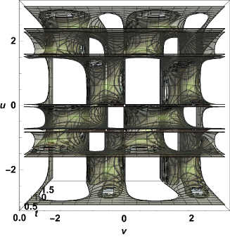
Figure 1: Representation of $\mathcal{S}$, as explained in Ref. [26].

This situation is very general and occurs in many cases. It applies mutas mutandis when the basic equation can only be deduced from (7_p).

b Real case

More generally, $\mathcal{S}$ is the universal classification surface of all systems, for which ($R$) is fulfilled. However, this does not imply that, in such systems, the singularities can be directly classified by $\pi_{1}(\mathcal{S})$, as it is in the very fortunate case of Lieb-kagome model.

c Generalized Haldane model on Lieb lattice

We introduce[34] the Bloch Hamiltonian

$$H_{\rm gH}=\hbar\pmatrix{0&\Omega_{1}\cos\frac{k_{x}}{2}&-\mathbbm{i}\Omega_{3}\cos\frac{k_{x}-k_{y}}{2}\cr\Omega_{1}\cos\frac{k_{x}}{2}&{\delta_{1}}&\Omega_{2}\cos\frac{k_{y}}{2}\cr\mathbbm{i}\Omega_{3}\cos\frac{k_{x}-k_{y}}{2}&\Omega_{2}\cos\frac{k_{y}}{2}&{\delta_{3}}\cr}$$

and will consider the case with $\Omega_{1}=\Omega_{2}=\Omega_{3}=1$.

The study of eigenvectors of $H_{\rm gH}$ reveals four singularities in the reciprocal space, $K_{0}$ corresponding to $(k_{x},k_{y})=(0,0)$, $K_{1}$ to $(0,\pi)$, $K_{2}$ to $(\pi,0)$ and $K_{3}$ to $(\pi,\pi)$, see Fig. 2. Contrary to Liev-kagome system, this one is not pathological and energy bands do not collapse. The four singularities are found from symmetry considerations[34] and their positions are confirmed independently by the hereby calculations. Hamiltonian $H_{\rm gH}$ does not respect symmetry ($R$), all components of eigenvectors are non-zero. They respect (7_a), so one can analyse its singularities in $s_{6}$; in this classification space, the system is faithfully represented by $(a_{4},a_{5},a_{6},a_{7},b_{4},b_{5},b_{6})$ and we write $X(k_{x},k_{y})=(a_{4}{\scriptstyle(k_{x},k_{y})},a_{5}{\scriptstyle(k_{x},k_{y})},a_{6}{\scriptstyle(k_{x},k_{y})},a_{7}{\scriptstyle(k_{x},k_{y})},b_{4}{\scriptstyle(k_{x},k_{y})},b_{5}{\scriptstyle(k_{x},k_{y})},b_{6}{\scriptstyle(k_{x},k_{y})})$.

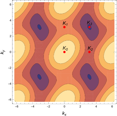
Figure 2: Contours of the highest eigenenergy of $H_{\rm gH}$ with $k_{x}$ and $k_{y}$ varying in $[-2\pi,2\pi]$. Discontinuities $K_{0}$, $K_{1}$, $K_{2}$ and $K_{3}$ are indicated. Both axis are necessarily $2\pi$-periodic but, according to the values of $({\delta_{1}},{\delta_{3}})$, the diagram can be $\pi$-periodic in $k_{x}$-direction or in $k_{y}$-direction or both or none. Here, $({\delta_{1}},{\delta_{3}})=(-\frac{1}{2},\frac{1}{2})$.

The exploration of singularity $K_{0}$ proves easy: let $\mathcal{C}_{0}$ be the circle described by $(k_{x},k_{y})=(\cos t,\sin t)$ and turning around $K_{0}$, one observes that the trajectory of $P_{t}=X(\cos t,\sin t)$ in $s_{6}$ is a loop with period $\pi$, as shown in Fig. 3; this means that $\mathcal{C}_{0}$ maps into a double loop, so $K_{0}$ corresponds to winding numbers $\omega_{0}=\pm 2$.

Figure 3: Plots of $\alpha_{i}(\cos t,\sin t)$ for $\alpha=a,b$ and $i=4..7$ (withdrawing $b_{7}$) for arbitrary values of $({\delta_{1}},{\delta_{3}})$, here $({\delta_{1}},{\delta_{3}})=({-}0.5,1.2)$.

Thus $P_{t+\pi}=P_{t}$ $\forall t$, which allows us to plot in Fig. 4 the distance[35] from $Q_{t}\equiv(P_{t}+P_{t+\frac{\pi}{2}})/2$ to $s_{6}$ versus $t$. It is always strictly positive, which proves that $Q_{t}$, which describes a continuous loop while $t$ varies from 0 to $\pi$, lies strictly outside of $s_{6}$. Since $Q_{t}$ is the isobarycentre of points $P_{t}$ and its half-period translate $P_{t+\frac{\pi}{2}}$, $P_{t}$ turns, while moving with the same parameter $t$, around $Q_{t}$, therefore the mapping $P_{t}$ turns around a hole in $s_{6}$. This hole cannot be closed, so this mapping is not contractible[36].

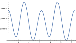
Figure 4: Plot of $|\widehat{7_{a}}(Q_{t})|$, the distance from $Q_{t}$ to $s_{6}$ for $t\in[0,2\pi]$ and arbitrary values of $({\delta_{1}},{\delta_{3}})$, here $({\delta_{1}},{\delta_{3}})=(0.5,0.3)$.

The hole defined above allows the determination of $\omega_{0}$. It is not only cylindrical: decreasing the radius of $\mathcal{C}_{0}$ down to zero, one finds that its shape is a six-dimensional multiple cone, which is pinched into a point $D_{0}$ at its centre, $D_{0}$ is the image of $K_{0}$. More generally, $\forall i=0,..,3$, one finds that all singularities $K_{i}$ can be classified by a multiple cone in $s_{6}$, pinched into a point $D_{i}$, which is the image of $K_{i}$.

For $({\delta_{1}},{\delta_{3}})=(\frac{1}{2},\frac{1}{2})$, $P_{t}$ turns around $(0.292,-0.52,-0.4,0.27,-0.58,0.1,-0.2)$. This determination depends on $({\delta_{1}},{\delta_{3}})$ and on the singularity $K_{i}$, with $i=0..3$. The situation is very intricate for cases $i\neq 0$, so we will only study the hole corresponding to singularity $K_{0}$. Also, the directions of the hole should be studied separately. One can map $P_{t}$ in $\tau_{1}(s_{6})$, the projection of $s_{6}$ in $(a_{4},a_{5},a_{6})$ coordinates: $\tau_{1}(P_{t})$ makes a double loop around a singularity of $\tau_{1}(s_{6})$, as shown in Fig. 5. In order to see the mapping of $\mathcal{C}_{0}$ more clearly, we have made a zoom in Fig 6.

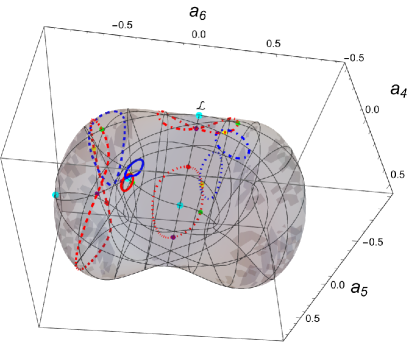
Figure 5: Representation of the mapping by $\tau_{1}$ of several circles of $(k_{x},k_{y})$-plane. $\tau_{1}(s_{6})$ is pinched along a line $\mathcal{L}$, which is indicated in the middle of the figure. Large cyan points represent $\tau_{1}(D_{i})$ for $i=1..4$, mappings are in red when the circle is around a singularity, in blue when it avoids it. Red, yellow, green and purple points follow this order in non-trivial paths but may overlap. Plain lines correspond to singularity $K_{0}$ ($\tau_{1}(D_{0})$ is a singularity of the surface, as shown in Fig. 6). Dotted lines correspond to singularity $K_{1}$; $\tau_{1}(D_{1})$ is at the middle of $\mathcal{L}$ and the non-trivial path crosses $\mathcal{L}$ twice. Dashed lines correspond to singularity $K_{2}$ (the 8-shape is artificially created by the two-dimensional projection of the drawing). Dot-dashed lines correspond to singularity $K_{3}$, one observes that the non-trivial one makes a loop with 8-shape, which collapses at one extremity of $\mathcal{L}$.

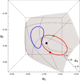
Figure 6: Mapping of two circles in $(k_{x},k_{y})$-plane, the first one turns around $K_{0}$ and maps into a loop turning twice around the singularity figured by a black point. Colored points follow the same order as in the previous figure. The second circle avoids $K_{0}$ and maps into a single loop, turning once and avoiding the black point, it is therefore trivial.

Let us move to the analysis of singularity $K_{1}$, which analysis proves much more involved than that of $K_{0}$. Let $\mathcal{C}_{1}$ be the circle described by $(k_{x},k_{y})=(\cos t,\pi+\sin t)$ and turning around $K_{1}$, one observes in Fig. 5 the projection of $R_{t}=X(\cos t,\pi+\sin t)$ in $\tau_{1}(s_{6})$. Loop $R_{t}$ is simple, this is confirmed in Fig. 7.

Figure 7: Plots of $\alpha_{i}(\cos t,\pi+\sin t)$ for $\alpha=a,b$ and $i=4..7$ (withdrawing $b_{7}$) for arbitrary values of $({\delta_{1}},{\delta_{3}})$, here $({\delta_{1}},{\delta_{3}})=({-}0.5,0.9)$.

Taking advantage of this, we plot the distance from $S^{\theta}_{t}\equiv\cos(\theta)^{2}R_{t}+\sin(\theta)^{2}R_{t+\pi}$ to $s_{6}$ versus $t$ in Fig. 8. Almost all values of $\theta$ can be chosen, giving a non-zero distance.

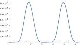
Figure 8: Plot of $|\widehat{7_{a}}(S^{1}_{t})|$, the distance from $S^{1}_{t}$ to $s_{6}$ for $t\in[0,2\pi]$, with $\theta=1$ and arbitrary values of $({\delta_{1}},{\delta_{3}})$, here $({\delta_{1}},{\delta_{3}})=(0.5,0.3)$.

However, this distance is zero for $t=0$ and $t=\pi$. Moreover, this plot gives a constant zero distance when $\theta=\frac{\pi}{4}$. This can be correlated to the crossing of line $\mathcal{L}$ observed in Fig. 5 and interpreted as a more complicated hole structure in $s_{6}$, which can be schematized by its orthogonal section in Fig. 9. This sketch provides indeed the configuration, for which the barycentre $S^{\theta}_{t}$ (constructed the same way than $Q_{t}$, taking into account the doubling of period and choosing weights $\cos(\theta)^{2}$ and $\sin(\theta)^{2}$ instead of uniform weights $\frac{1}{2}$) joins surface $s_{6}$ twice, while $S^{\pi/4}_{t}$ always lies in $s_{6}$.

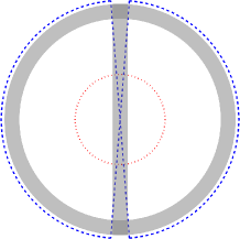
Figure 9: Sketch of the orthogonal section of the hole structure, corresponding to singularity $K_{2}$. The dashed line stands for $R_{t}$, one observes that the hole divides into two separate holes, which frontier is flat (at least in some dimensions). The dotted line stands for $S^{1}_{t}$.

The non triviality of $R_{t}$ is established by the two holes, with the same confidence than that of $P_{t}$. Altogether, we have established that $K_{1}$ corresponds to winding numbers $\omega_{1}=\pm 1$.

Let us move to the analysis of singularity $K_{2}$. Let $\mathcal{C}_{2}$ be the circle described by $(k_{x},k_{y})=(\pi+\cos t,\sin t)$ and turning around $K_{2}$, one observes in Fig. 5 the projection of $T_{t}=X(\pi+\cos t,\sin t)$ in $\tau_{1}(s_{6})$. Loop $T_{t}$ is simple, this is confirmed in Fig. 10.

Figure 10: Plots of $\alpha_{i}(\pi+\cos t,\sin t)$ for $\alpha=a,b$ and $i=4..7$ (withdrawing $b_{7}$) for arbitrary values of $({\delta_{1}},{\delta_{3}})$, here $({\delta_{1}},{\delta_{3}})=(0.5,0.9)$.

Taking advantage of this, we plot the distance from $U_{t}\equiv(T_{t}+T_{t+\pi})/2$ to $s_{6}$ versus $t$ in Fig. 11. It is always strictly positive and indicates that the mapping $T_{t}$ turns around a hole in $s_{6}$ (using the same argument used for $P_{t}$, while taking into account the doubling of period). The non triviality of $T_{t}$ is established with the same confidence than that of $P_{t}$. Altogether, we have established that $K_{2}$ corresponds to winding numbers $\omega_{2}=\pm 1$.

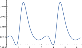
Figure 11: Plot of $|\widehat{7_{a}}(U_{t})|$, the distance from $U_{t}$ to $s_{6}$ for $t\in[0,2\pi]$ and arbitrary values of $({\delta_{1}},{\delta_{3}})$, here $({\delta_{1}},{\delta_{3}})=(0.5,0.3)$.

Let us move to the analysis of singularity $K_{3}$. Let $\mathcal{C}_{3}$ be the circle described by $(k_{x},k_{y})=(\pi+\cos t,\pi+\sin t)$ and turning around $K_{2}$, one observes in Fig. 5 the projection of $V_{t}=X(\pi+\cos t,\pi+\sin t)$ in $\tau_{1}(s_{6})$. Loop $V_{t}$ is simple, this is confirmed in Fig. 12.

Figure 12: Plots of $\alpha_{i}(\pi+\cos t,\pi+\sin t)$ for $\alpha=a,b$ and $i=4..7$ (withdrawing $b_{7}$) for arbitrary values of $({\delta_{1}},{\delta_{3}})$, here $({\delta_{1}},{\delta_{3}})=({-}0.5,0.9)$.

Taking advantage of this, we plot the distance from $W_{t}\equiv(V_{t}+V_{t+\pi})/2$ to $s_{6}$ versus $t$ in Fig. 13.

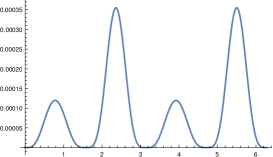
Figure 13: Plot of $|\widehat{7_{a}}(W_{t})|$, the distance from $W_{t}$ to $s_{6}$ for $t\in[0,2\pi]$, and arbitrary values of $({\delta_{1}},{\delta_{3}})$, here $({\delta_{1}},{\delta_{3}})=(0.5,0.3)$.

This distance is always strictly positive, except for $t=n\frac{\pi}{2}$ $\forall n\in\mathbb{Z}$ at which points it is zero. In order to interpret the structure, we have also checked that $W_{t}^{\theta}$ is distant of $s_{6}$ $\forall\theta\in[0,2\pi[$ and $\forall t\neq n\frac{\pi}{2}$ with $n\in\mathbb{Z}$ ($W_{t}^{\theta}$ is defined exactly as $S_{t}^{\theta}$). This can be correlated to the 8-shaped observed in Fig. 5 and interpreted as a more complicated hole structure in $s_{6}$, which can be schematized by its orthogonal section in Fig. 14. This sketch provides indeed the configuration, for which the isobarycentre $W_{t}$ (constructed the same way than $Q_{t}$, taking into account the doubling of period) joins surface $s_{6}$ four times.

Figure 14: Sketch of the orthogonal section of the hole structure, represented by a circle with radius $r$, corresponding to singularity $K_{3}$. The blue dashed line (outside of the plain circle) stands for $V_{t}$, the dashed line between points $(0,r)$ and $(0,-r)$ represents an attachment, these points are merged into a unique one, and so are points $(r,0)$ and $(-r,0)$.

The non triviality of $V_{t}$ is established by the hole sketched in Fig. 14, with the same confidence than that of $P_{t}$. Altogether, we have established that $K_{3}$ corresponds to winding numbers $\omega_{3}=\pm 1$.

We would like to address now the question of the sign $s^{i}({\delta_{1}},{\delta_{3}})$ of $\omega_{i}$. Its determination $s_{\rm r}^{i}({\delta_{1}},{\delta_{3}})$ through a classification surface like $s_{6}$ is only relative and a global sign $\varepsilon$ must be defined elsewhere, such that $s^{i}({\delta_{1}},{\delta_{3}})=\varepsilon s_{\rm r}^{i}({\delta_{1}},{\delta_{3}})$. For singularity $K_{0}$, $s_{\rm r}^{0}({\delta_{1}},{\delta_{3}})=1$ is trivial, as seen by comparing the turning directions of all path $\tau_{1}(P_{t})$ when $({\delta_{1}},{\delta_{3}})$ varies. This is confirmed by analysing in detail all copies of Fig. 3 for various values of $({\delta_{1}},{\delta_{3}})$.

For singularity $K_{1}$, a change of sign is manifest at the bottom frontier drawn in Fig.19 but we could not get to a definitive proof. A huge inconvenient of the representation chosen in Fig. 5 is that the surface on which all circles are mapped is $({\delta_{1}},{\delta_{3}})$ dependant. There exist universal representations onto which one could map all projections but we could not achieve their determination yet[37]. Instead, we have found that both projections $\Pi_{\rm odd}$ and $\Pi_{\rm even}$, defined by putting, respectively, $(a_{4},a_{6},b_{4},b_{6})\to(0,0,0,0)$ and $(a_{5},a_{7},b_{5},b_{7})\to(0,0,0,0)$ in (7_p), gives the same universal equation

$$3x\,z(y+z)^{2}=z\,w(y(3-x)+z(3+z))\,.$$ (8)

More precisely, $\Pi_{\rm odd}(\widehat{\hbox{\ref{eq47}}})=0$ gives (8) with $x={a_{5}}^{2}+{a_{7}}^{2}$, $y={b_{5}}^{2}+{b_{7}}^{2}$, $z=a_{5}b_{5}+a_{7}b_{7}$ and $w=(a_{7}b_{5}-a_{5}b_{7})^{2}$, while $\Pi_{\rm even}(\widehat{\hbox{\ref{eq47}}})=0$ gives (8) with $x={a_{4}}^{2}+{a_{6}}^{2}$, $y={b_{4}}^{2}+{b_{6}}^{2}$, $z=a_{4}b_{4}+a_{6}b_{6}$ and $w=(a_{6}b_{4}-a_{4}b_{6})^{2}$. We write $s_{3}$ the surface corresponding to (8) and show a 3-dimensional representation of $s_{3}$ in Fig. 15.

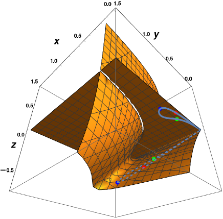
Figure 15: Representation of $s_{3}$, putting $w=\frac{9}{16}$, its maximal value. From the definitions of $\alpha_{i}$ components, with $\alpha=a,b$ and $i=4..7$, $x$ and $y$ range in $[0,\frac{3}{2}]$ while $z$ ranges in $[-\frac{3}{4},\frac{3}{4}]$. We represent two paths obtained by the $\Pi_{\rm odd}$ projection, the dashed line with $({\delta_{1}},{\delta_{3}})=(\frac{1}{2},-\frac{1}{2})$, the plain one with $({\delta_{1}},{\delta_{3}})=(-\frac{1}{2},\frac{1}{2})$, the mappings follow the order $\color[rgb]{0,0,1}\bullet\color[rgb]{1,0,0}\bullet\color[rgb]{0,1,0}\bullet$. They are close to different folds, with the same apparent orientation, although, moving one path continuously to the orther would give the opposite orientation.

$\Pi_{\rm odd}(R_{t})$ and $\Pi_{\rm even}(R_{t})$ are found $\pi$-periodic, as shown in Fig. 16.

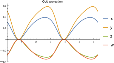
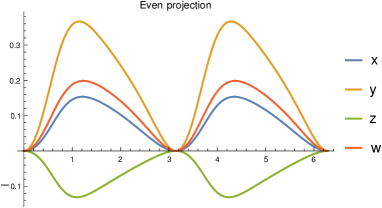
Figure 16: Plot of $\Pi_{\rm odd}(R_{t})$ versus $t$ (left) and $\Pi_{\rm even}(R_{t})$ versus $t$ (right) for $t\in[0,2\pi]$ and arbitrary values of $({\delta_{1}},{\delta_{3}})$, here $({\delta_{1}},{\delta_{3}})=(0.5,0.3)$. Be careful that definitions of $(x,y,z,w)$ are different for $\Pi_{\rm odd}$ and $\Pi_{\rm even}$.

This projections are not canonical, indeed neither $\Pi_{\rm odd}(R_{t})$ nor $\Pi_{\rm even}(R_{t})$ do map exactly on (8). However, by chance, they are close to it. Actually $\{\Pi_{\rm odd}(R_{0}),\Pi_{\rm even}(R_{0}),\Pi_{\rm odd}(R_{\frac{\pi}{2}}),\Pi_{\rm even}(R_{\frac{\pi}{2}})\}\subset s_{3}$, which one shows by plotting $\Pi_{\rm odd}(\widehat{\hbox{\ref{univ}}}(R_{t}))$ and $\Pi_{\rm even}(\widehat{\hbox{\ref{univ}}}(R_{t}))$, in Fig. 17. One finds two close leaves in Fig. 15, which are inversely orientated, from a topological point of view. Each path moves from one leaf to the other, keeping the same apparent orientation, when $({\delta_{1}},{\delta_{3}})$ approaches the bottom frontier line of Fig. 19. So, their effective orientation must be reversed when crossing this line.

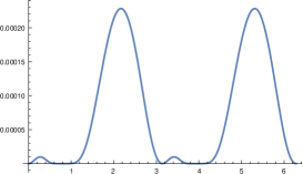
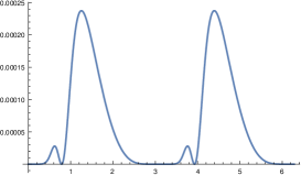
Figure 17: Plot of $\Pi_{\rm odd}(\widehat{\hbox{\ref{univ}}}(R_{t}))$ versus $t$ (left) and $\Pi_{\rm even}(\widehat{\hbox{\ref{univ}}}(R_{t}))$ versus $t$ (right) for $t\in[0,2\pi]$ and arbitrary values of $({\delta_{1}},{\delta_{3}})$, here $({\delta_{1}},{\delta_{3}})=(0.5,-0.9)$. Be careful that definitions of $(x,y,z,w)$ are different for $\Pi_{\rm odd}$ and $\Pi_{\rm even}$.

It seems that $z$ drives the change of sign of the orientation. This is confirmed by the contours of $z=a_{5}b_{5}+a_{7}b_{7}$ which fits one of the frontiers shown in Fig. 18.

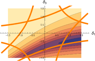
Figure 18: Contours of $a_{5}{\scriptstyle(k_{x},k_{y})}b_{5}{\scriptstyle(k_{x},k_{y})}+a_{7}{\scriptstyle(k_{x},k_{y})}b_{7}{\scriptstyle(k_{x},k_{y})}$, with $t=0.2$ and $(k_{x},k_{y})=(\cos t,\pi+\sin t)$. ${\delta_{1}}$ and ${\delta_{3}}$ vary in $[-\frac{3}{2},\frac{3}{2}]$ and the frontiers of Fig. 19 are indicated.

We must now compare our results to those in [34]. In Fig. 19, we show the frontiers that have been found. We added the contours of $\cot(\theta)=\sqrt{4p({\delta_{1}},{\delta_{3}})^{3}/q({\delta_{1}},{\delta_{3}})^{2}-1}$, with $p(x,y)=9+x^{2}-xy+y^{2}$ and $q(x,y)=2x^{3}-3x^{2}y-3x\,y^{2}+2y^{3}$, which is related to an angle $\theta$, the cotangent of which fits exactly these frontiers. $\theta$ is directly related to the eigenenergies of this model, which are $\frac{{\delta_{1}}+{\delta_{3}}}{2}+\frac{2}{3}\sqrt{p({\delta_{1}},{\delta_{3}})}\cos(\frac{\theta+\varepsilon\pi}{3})$ with $\varepsilon=-1,0,1$.

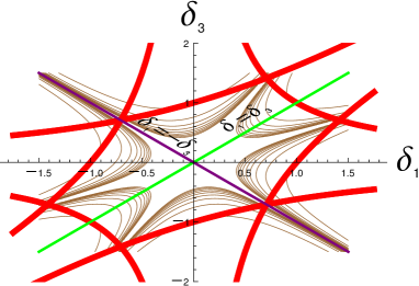
Figure 19: Frontiers in the map of winding parameters versus $({\delta_{1}},{\delta_{3}})$. The first and second bisectors are also indicated.

In [34], the authors find a winding number $\omega=\pm 4$, which sign changes in the different areas designed by the frontiers of Fig. .19. The combination of two windings $\pm 1$ can give an effective winding of $\pm 2$ and, similarly, the combination of two windings $\pm 2$ can give an effective winding of $\pm 4$; therefore, some combinations of $\omega_{0}$, $\omega_{1}$, $\omega_{2}$ or $\omega_{3}$ give indeed an effective winding number of $\pm 4$. On the other hand, classifying singularities through surface $s_{6}$ gives exhaustively all primary winding numbers, so $\omega$ must be some of these combinations. Moreover, since $\omega$ has different signs in the different areas, described in Fig. 19, the related changes of sign must inherit from that of some $\omega_{i}$, $i=0..3$; in particular, this reinforces our interpretation of a sign change for $\omega_{1}$. But this determination remains currently questionable and we have renounced to study the signs of $\omega_{2}$ and $\omega_{3}$. Eventually, one must find a more robust method to solve this very interesting question, from which it will be possible to deduce the relations between $\omega$ and the other $\omega_{i}$, $i=0..3$.

Eventually, we deal with an atypical case in the following.

d Lieb model

This model[38, 39, 40] is extraordinary for several reasons. Its classification surface is circle $S_{1}$ and the corresponding basic equation is thus atypical. It corresponds to Lieb-kagome parameter $t^{\prime}=0$ and separates from the general Lieb-kagome surface $\mathcal{S}$, which holds when $0<t^{\prime}\leq 1$; fortunately, we could find surface $\widetilde{\mathcal{S}_{1}}$, which is valid both in Lieb and Lieb-kagome cases[26, 41], i.e. $\forall t^{\prime}\in[0,1]$. Investigating loops while varying continuously $t^{\prime}$ allows one to understand why winding numbers tend to $\pm 2$ when $t^{\prime}\to 0$, though the exact $t^{\prime}=0$ limit, calculated in $S_{1}$, is $\pm 1$: $\widetilde{\mathcal{S}_{1}}$ consists essentially in two planes, into which each path around a singularity makes a single loop (which by definition corresponds to winding number 1). When the limit $t^{\prime}=0$ is reached, these planes merge, so that winding numbers fuse and do not add; thus, this apparent anomaly is explained.

This example seems to indicate that atypical cases arise when the system follows additional symmetries. In the Lieb case, there is indeed a three-fold degeneracy of eigenvalues, which is very exceptional.

6 Conclusion

It is wonderful that the topological singularities of almost any three-band hamiltonian can be mapped onto the same universal surface $s_{6}$. Although one is not assured to characterize winding numbers in this surface, it contains all subsurfaces in which they can be defined. Some cases, not following (7_a), do follow another $(e_{i\alpha})$ but, as we believe, it is more efficient to establish a unique couple of (basic,parent) equations: eventually, one gets only four different equations (7_a), (7_p), ($S_{2}$) and ($S_{4}$) which cover all cases[42].

This extends a similar result in real case: $\mathcal{S}$ is universal for almost all three-band hamiltonian respecting ($R$), but its structure is much easier to investigate from Fig. 1.

It is not known yet, whether atypical cases have physical applications, but one can observe that the fourth one (for which general parametrization rules $\mathcal{R}$, defined in appendix, hold) exactly generalizes the two-band unique solution.

The way universal classification surfaces are constructed seems to exclude the influence of each hamiltonian properties in the determination of singularities but this is a wrong interpretation. Hamiltonians directly govern the way paths are constructed in $s_{6}$. Also, their symmetries are responsible for the reduction from $s_{6}$ to their effective classification surface. However, in the Lieb-kagome example, it is true that winding numbers can be immediately determined in $\mathcal{S}$ and probably in $s_{6}$ too.

A further simple investigation shall be to study the mapping of paths, defined in reciprocal space for Lieb-kagome model, into $s_{6}$, with the hope to determine a part of its fundamental group.

Eventually, one observes that ($\gamma$) is true in any case. For systems following ($R$) condition, ($\gamma$) becomes trivial. We have no physical interpretation of this condition yet and it will be very interesting to study it for specific hamiltonians not following ($R$) as $H_{\rm gH}$.

Appendix

a Definition of the $\star$ product

Let $a=(a_{i})_{i=1..8}$ and $b=(b_{i})_{i=1..8}$, two vectors of the $\mathbb{R}^{8}$ space, the star product $a\star b$ is defined[28, 26] by $a\star b=\sum_{i=1}^{8}a^{j}b^{k}d_{ijk}$ with

$$d_{ii8}=d_{i8i}=d_{8ii}=\frac{1}{\sqrt{3}}\qquad\forall i=1,2,3\;;$$

$$d_{ii8}=d_{i8i}=d_{8ii}={-}\frac{1}{2\sqrt{3}}\quad\forall i=4,..,7\;;$$

$$d_{888}={-}\frac{1}{\sqrt{3}}\;;$$

$$d_{146}=d_{461}=d_{614}=d_{164}=d_{641}=d_{416}=\frac{1}{2}\;;$$

$$d_{157}=d_{571}=d_{715}=d_{175}=d_{751}=d_{517}=\frac{1}{2}\;;$$

$$d_{256}=d_{562}=d_{625}=d_{265}=d_{652}=d_{526}=\frac{1}{2}\;;$$

$$d_{344}=d_{434}=d_{443}=d_{355}=d_{535}=d_{553}=\frac{1}{2}\;;$$

$$d_{247}=d_{472}=d_{724}=d_{274}=d_{742}=d_{427}={-}\frac{1}{2}\;;$$

$$d_{366}=d_{636}=d_{663}=d_{377}=d_{737}=d_{773}={-}\frac{1}{2}\;.$$

b Explicit expressions of universal surface $s_{6}$

The explicit expression of (7_p) is

$$({a_{4}}^{2}+{a_{5}}^{2}+{a_{6}}^{2}+{a_{7}}^{2})(a_{4}b_{4}+{b_{4}}^{2}+a_{5}b_{5}+{b_{5}}^{2}+a_{6}b_{6}+{b_{6}}^{2}+a_{7}b_{7}+{b_{7}}^{2})\times$$

$$\!\!\!\!\!\!\!\!\!\!\!\!\!\!\!\!\Bigg{(}({a_{4}}^{2}+{a_{5}}^{2})({b_{4}}^{2}+{b_{5}}^{2})+({a_{6}}^{2}+{a_{7}}^{2})({b_{6}}^{2}+{b_{7}}^{2})+(a_{4}b_{4}+a_{5}b_{5}+a_{6}b_{6}+a_{7}b_{7})\times$$

$$\!\!\!\!\!\!\!\!\!\!\!\!\!\!\!\!\!\!\!\!\!\!\!\!({b_{4}}^{2}+{b_{5}}^{2}+{b_{6}}^{2}+{b_{7}}^{2})+2\bigg{(}(a_{5}b_{4}-a_{4}b_{5})(a_{7}b_{6}-a_{6}b_{7})+(a_{4}b_{4}+a_{5}b_{5})(a_{6}b_{6}+a_{7}b_{7})\bigg{)}\Bigg{)}$$

$$=\Bigg{(}({a_{6}}^{2}+{a_{7}}^{2})({b_{4}}^{2}+{b_{5}}^{2})+({a_{4}}^{2}+{a_{5}}^{2})({b_{6}}^{2}+{b_{7}}^{2})$$

$$-2\bigg{(}(a_{5}b_{4}-a_{4}b_{5})(a_{7}b_{6}-a_{6}b_{7})+(a_{4}b_{4}+a_{5}b_{5})(a_{6}b_{6}+a_{7}b_{7})\bigg{)}\Bigg{)}\times$$

$$\!\!\!\!\!\!\!\!\!\!\!\!\!\!\!\!\Bigg{[}(3+a_{4}b_{4}+a_{5}b_{5}+a_{6}b_{6}+a_{7}b_{7})\times\Bigg{(}({a_{4}}^{2}+{a_{5}}^{2})({b_{4}}^{2}+{b_{5}}^{2})+({a_{6}}^{2}+{a_{7}}^{2})({b_{6}}^{2}+{b_{7}}^{2})$$

$$+2\bigg{(}(a_{5}b_{4}-a_{4}b_{5})(a_{7}b_{6}-a_{6}b_{7})+(a_{4}b_{4}+a_{5}b_{5})(a_{6}b_{6}+a_{7}b_{7})\bigg{)}\Bigg{)}$$

$$\!\!\!\!\!\!\!\!\!\!\!\!\!\!\!\!-\bigg{(}(-3+{a_{4}}^{2}+{a_{5}}^{2}+{a_{6}}^{2}+{a_{7}}^{2})(a_{4}b_{4}+a_{5}b_{5}+a_{6}b_{6}+a_{7}b_{7})({b_{4}}^{2}+{b_{5}}^{2}+{b_{6}}^{2}+{b_{7}}^{2})\bigg{)}\Bigg{]}.$$

The explicit expression of (7_a) and thus the equation of $s_{6}$ is

$$\!\!\!\!\!\!\!\!\!\!\!\!\!\!\!\!3({a_{4}}^{2}+{a_{5}}^{2}+{a_{6}}^{2}+{a_{7}}^{2})\Bigg{(}{a_{6}}^{2}\bigg{(}b_{4}(a_{4}+b_{4})+b_{5}(a_{5}+b_{5})\bigg{)}+({a_{6}}^{2}+{a_{7}}^{2})b_{6}(a_{6}+b_{6})$$

$$+(a_{5}b_{4}-a_{4}b_{5})(a_{6}a_{7}+a_{5}b_{4}-a_{4}b_{5}+2a_{7}b_{6})\Bigg{)}^{2}$$

$$\!\!\!\!\!\!\!\!\!\!\!\!\!\!\!\!\!\!\!\!\!\!\!\!\!\!\!\!\!\!\!\!=\Bigg{(}({a_{4}}^{2}+{a_{5}}^{2}+2{a_{6}}^{2})(a_{5}b_{4}-a_{4}b_{5})^{2}-2a_{7}(-a_{5}b_{4}+a_{4}b_{5})\bigg{(}({a_{4}}^{2}+{a_{5}}^{2})b_{6}-a_{6}(a_{4}b_{4}+a_{5}b_{5})\bigg{)}$$

$$+({a_{6}}^{2}+{a_{7}}^{2})\bigg{(}{a_{6}}^{2}({b_{4}}^{2}+{b_{5}}^{2})-2a_{6}(a_{4}b_{4}+a_{5}b_{5})b_{6}+({a_{4}}^{2}+{a_{5}}^{2}){b_{6}}^{2}\bigg{)}\Bigg{)}\times$$

$$\Bigg{(}\bigg{(}a_{4}a_{6}b_{4}+a_{5}a_{7}b_{4}+a_{5}a_{6}b_{5}-a_{4}a_{7}b_{5}+({a_{6}}^{2}+{a_{7}}^{2})b_{6}\bigg{)}\times$$

$$\bigg{(}a_{6}(3+a_{4}b_{4}+a_{5}b_{5})+{a_{6}}^{2}b_{6}+a_{7}(a_{5}b_{4}-a_{4}b_{5}+a_{7}b_{6})\bigg{)}$$

$$\!\!\!\!\!\!\!\!\!\!\!\!\!\!\!\!-(-3+{a_{4}}^{2}+{a_{5}}^{2}+{a_{6}}^{2}+{a_{7}}^{2})\bigg{(}(a_{5}b_{4}-a_{4}b_{5}+a_{7}b_{6})^{2}+{a_{6}}^{2}({b_{4}}^{2}+{b_{5}}^{2}+{b_{6}}^{2})\bigg{)}\Bigg{)}.$$

c Subcases

We study what happens when $a_{i}$ follow additional conditions in more details, through some examples, but we exclude atypical cases.

Let’s consider a system obeying additional conditions ${\chi_{1}}_{a}=0=a_{4}b_{i}+a_{i}b_{4}$, $i=6,7$. Its basic equation becomes $(x_{1})$ $3\widetilde{A}_{a}({{A{\scriptstyle 2}}_{a}}^{2}(a_{4}-b_{4})^{2}-{{A{\scriptstyle 1}}_{a}}^{2}(a_{4}+b_{4})^{2})=16{b_{4}}^{2}{{A{\scriptstyle 1}}_{a}}^{2}{{A{\scriptstyle 2}}_{a}}^{2}$ and follows basic equation (7_a) since $\widehat{x_{1}}=\frac{{a_{4}}^{4}}{{a_{6}}^{4}{b_{4}}^{2}}\widehat{7_{a}}\rfloor_{b_{5}\to\frac{b_{4}a_{5}}{a_{4}},b_{6}\to-\frac{b_{4}a_{6}}{a_{4}},b_{7}\to-\frac{b_{4}a_{7}}{a_{4}}}$. There are 5 degrees of freedom $(a_{i})_{i=4..7}$ and $b_{4}$ and the parametrization of other ones reads $a_{1}=-\frac{4b_{4}{A{\scriptscriptstyle 1}}_{a}{A{\scriptscriptstyle 2}}_{a}{\eta_{1}}_{\!a}}{{\scriptscriptstyle\sqrt{3}}\widetilde{A}_{a}x_{a}}$, $a_{2}=-\frac{{\eta_{2}}_{\!a}}{{\eta_{1}}_{\!a}}a_{1}$, $a_{3}=-\frac{2b_{4}{A{\scriptscriptstyle 1}}_{a}{A{\scriptscriptstyle 2}}_{a}}{{\scriptscriptstyle\sqrt{3}}\,x_{a}}$, $b_{i}=-\frac{{b_{4}}^{2}}{{a_{4}}^{2}}a_{i}$ $\forall i=1..3$, $b_{i}=-\frac{b_{4}}{a_{4}}a_{i}$ $\forall i=6,7$, $b_{5}=\frac{b_{4}a_{5}}{a_{4}}$, $a_{8}=-\frac{1}{2}+\frac{3((a_{4}+b_{4}){{A{\scriptscriptstyle 1}}_{a}}^{2}-(a_{4}-b_{4}){{A{\scriptscriptstyle 2}}_{a}}^{2})}{8b_{4}{A{\scriptscriptstyle 1}}_{a}{A{\scriptscriptstyle 2}}_{a}}$ and $b_{8}=\frac{1}{2}-\frac{2{b_{4}}^{2}{A{\scriptscriptstyle 1}}_{a}{A{\scriptscriptstyle 2}}_{a}}{a_{4}x_{a}}$.

If condition $a_{6}=b_{6}=0$ is added to the previous condition, the basic equation of the system becomes $(x_{2})$ $3{A{\scriptstyle 3}}_{a}({a_{7}}^{2}(a_{4}-b_{4})^{2}-{{A{\scriptstyle 1}}_{a}}^{2}(a_{4}+b_{4})^{2})=16{a_{7}}^{4}{b_{4}}^{2}{{A{\scriptstyle 1}}_{a}}^{2}$ with $\widehat{x_{2}}=\frac{{a_{4}}^{5}}{{b_{4}}^{3}{A{\scriptscriptstyle 3}}_{a}}\widehat{7_{p}}\rfloor_{b_{5}\to\frac{b_{4}a_{5}}{a_{4}},a_{6}\to 0,b_{6}\to 0,b_{7}\to-\frac{b_{4}a_{7}}{a_{4}}}$, where ${A{\scriptstyle 3}}_{a}={A{\scriptstyle 1}}_{a}-{a_{7}}^{2}$, and does not follow basic equation (7_a) but its parent equation (7_p). There are 4 degrees of freedom $(a_{4},a_{5},a_{7},b_{4})$ and the parametrization of other ones reads $a_{1}=\frac{{\scriptscriptstyle\sqrt{3}}a_{5}y_{a}}{4a_{7}b_{4}{A{\scriptscriptstyle 1}}_{a}}$, $a_{2}=-\frac{{\scriptscriptstyle\sqrt{3}}a_{4}y_{a}}{4a_{7}b_{4}{A{\scriptscriptstyle 1}}_{a}}$, $a_{3}=\frac{{\scriptscriptstyle\sqrt{3}}{A{\scriptscriptstyle 3}}_{a}y_{a}}{8{a_{7}}^{2}b_{4}{A{\scriptscriptstyle 1}}_{a}}$, $b_{1}=\frac{4a_{5}{a_{7}}^{3}{b_{4}}^{2}{A{\scriptscriptstyle 1}}_{a}}{{\scriptscriptstyle\sqrt{3}}\,a_{4}{A{\scriptscriptstyle 3}}_{a}y_{a}}$, $b_{2}=-\frac{4{a_{7}}^{3}{b_{4}}^{2}{A{\scriptscriptstyle 1}}_{a}}{{\scriptscriptstyle\sqrt{3}}{A{\scriptscriptstyle 3}}_{a}y_{a}}$, $b_{3}=-\frac{2{a_{7}}^{2}{b_{a}}^{2}{A{\scriptscriptstyle 1}}_{a}}{{\scriptscriptstyle\sqrt{3}}\,a_{4}y_{a}},b_{5}=\frac{b_{4}a_{5}}{a_{4}}$, $b_{7}=-\frac{b_{4}a_{7}}{a_{4}}$, $a_{8}=\frac{1}{2}-\frac{2{a_{7}}^{2}b_{4}{A{\scriptscriptstyle 1}}_{a}}{y_{a}}$ and $b_{8}=\frac{1}{2}+\frac{3{A{\scriptscriptstyle 3}}_{a}y_{a}}{8a_{4}{a_{7}}^{2}{A{\scriptscriptstyle 1}}_{a}}$.

If a third condition $a_{7}=b_{7}$ is added, the system follows $b_{i}={-}a_{i}$ $\forall i=4,5$ and $b_{i}=a_{i}$ $\forall i=6,7$. Its basic equation reads $(x_{3})$ ${A{\scriptstyle 1}}_{a}(3-{A{\scriptstyle 1}}_{a})=3{a_{7}}^{2}$ with $\widehat{x_{3}}=\frac{1}{4{a_{4}}^{2}{a_{7}}^{4}}\widehat{x_{2}}\rfloor_{b_{4}\to a_{4}}=\frac{1}{4{a_{7}}^{4}{A{\scriptscriptstyle 3}}_{a}}\widehat{7_{p}}\rfloor^{a_{6}\to 0,b_{6}\to 0,b_{7}\to a_{7}}_{b_{4}\to-a_{4},b_{5}\to-a_{5}}$. There are 3 degrees of freedom $(a_{4},a_{5},a_{7})$ and the parametrization of other ones reads $a_{1}=\frac{2a_{5}a_{7}{A{\scriptscriptstyle 1}}_{a}}{{\scriptscriptstyle\sqrt{3}}{A{\scriptscriptstyle 3}}_{a}}$, $a_{2}=-\frac{a_{4}}{a_{5}}a_{1}$, $a_{3}=\frac{{A{\scriptscriptstyle 1}}_{a}}{{\scriptscriptstyle\sqrt{3}}}$, $b_{i}=a_{i}$ $\forall i=1..3$, $a_{8}=-\frac{1}{4}+\frac{3{a_{7}}^{2}}{4{A{\scriptscriptstyle 1}}_{a}}$ and $b_{8}=a_{8}$.

These examples demonstrate the sophistication of algebraic manipulations. Associativity of the composition of conditions is valid to deduce basic equations (although a surprising additional factor $\frac{{a_{4}}^{3}}{{b_{4}}^{3}}$ emerges depending on the way the last equation is constructed). But the parametrization is completely different for each case and associativity cannot be used to deduce it, because the parametrization of the reduced systems differs from that of the complete one (when projecting this one following the same conditions). The only way to obtain the correct parametrization is to use rules $\mathcal{R}$:

$$\!\!\!\!\!\!\!\!\!\!\!\!\forall i=1,2\hbox{ and }\forall\alpha=a,b\qquad\alpha_{i}=(-1)^{i}\frac{\sqrt{3}\,{\eta_{i}}_{\alpha}}{2\alpha_{8}-1}\hbox{ and }\alpha_{3}=\frac{\sqrt{3}\widetilde{A}_{\alpha}}{2(1-2\alpha_{8})}, \mathcal{R}$$ ()

which are always valid, except for the two first atypical cases giving $s_{2}$; they are also only partially valid for the third atypical case. In addition to $\mathcal{R}$ rules, one must substitute $a_{8}$ and $b_{8}$, using specific rules according to each case.

Eventually, one must be aware that a basic equation can be obtained with two different parametrizations, defining two separate cases. This occurs for atypical cases but also in general.

References

References

- [1] N. Read & D. Green, Phys. Rev. B 61, 10267 (2000).
- [2] A. Y. Kitaev, Phys. Usp. 44, 131 (2001).
- [3] L. Fu, C. L. Kane & E. S. Mele, Phys. Rev. Lett. 98, 106803 (2007).
- [4] C. Bena & G. Montambaux, New J. Phys. 11, 095003 (2009).
- [5] J.-N. Fuchs, F. Piéchon, M. O. Goerbig & G. Montambaux, Eur. Phys. J. B 77, 351 (2010).
- [6] L.-K. Lim, J.-N. Fuchs & G. Montambaux, Phys. Rev. A 92, 063627 (2015).
- [7] N. Read, Phys. Rev. Lett. 65, 1502 (1990).
- [8] F. Wilczek, Phys. Rev. Lett. 49, 957 (1982).
- [9] F. D. M. Haldane, Phys. Rev. Lett. 61, 2015 (1988).
- [10] C. N. Yang, Rev. Mod. Phys. 34, 694 (1962).
- [11] S. M. Girvin & A. H. MacDonald, Phys. Rev. Lett. 58, 1252 (1987).
- [12] S. C. Zhang, T. H. Hansson & S. Kivelson, Phys. Rev. Lett. 62, 82 (1989).
- [13] Z. F. Ezawa and A. Iwazaki, Phys. Rev. B 43, 2637 (1991).
- [14] Y. Tanaka, T. Yokoyama & N. Nagaosa, Phys. Rev. Lett. 103, 107002 (2009).
- [15] N. Regnault & B. A. Bernevig, Phys. Rev. X 1, 021014 (2011).
- [16] see refs. in: M. Z. Hasan & C. L. Kane, Rev. Mod. Phys. 82, 3045 (2010).
- [17] C. Liu et al., Nat. Mater. 19, 522 (2020) and refs. inside.
- [18] see refs. in: C. Nayak et al., Rev. Mod. Phys. 80, 1083 (2008).
- [19] H. Bartolomei, M. Kumar, R. Bisognin, A. Marguerite, J.-M. Berroir, E. Bocquillon, B. Plaçais, A. Cavanna, Q. Dong, U. Gennser, Y. Lin & G. Fève, Science 368, 173 (2020).
- [20] J. Nakamura, S. Liang, G. C. Gardner, M. Manfra, Nat. Phys. 16, 931 (2020).
- [21] H. A. Trung & B. Yang, Phys. Rev. Lett. 127, 046402 (2021).
- [22] C. B. Allendoerfer, Amer. J. Math. 62, 243 (1942).
- [23] W. Fenchel, J. London Math. Soc. 15, 15 (1940).
- [24] S.-S. Chern, Ann. Math. 45, 747 (1944).
- [25] G. Abramovici & P. Kalugin, Int. J. Geom. Methods Mod. Phys. 9, 1250023 (2012).
- [26] G. Abramovici, Eur. Phys. J. B 94, 132 (2021).
- [27] P. R. Wallace, Phys. Rev. 71, p622 (1947).
- [28] S. K. Goyal et al., J Phys. A: Math. Theor. 49, 165203 (2016).
- [29] Some real factors have no real roots and can be discarded. Other factors correspond to atypical cases, which are treated apart. We have eventually dealt with all general prime factors.
- [30] G. Abramovici, “Détails du calcul de la surface classifiante pour les systèmes hamiltoniens à 3 bandes”, (2022) hal-03708828.
- [31] One observes that some projections of have singular points but not , so should be a flag variety. Since is constructed as the quotient of by relations (5) and (2), it may be isomorphic to the complete flag variety . One needs to prove that these relations give the folding rules of a torus , but it exceeds the aims and possibilities of this article.
- [32] G. Montambaux, L.-K. Lim, J.-N. Fuchs & F. Piéchon, Phys. Rev. Lett. 121, 256402 (2018).
- [33] L.-K. Lim, J.-N. Fuchs, F. Piéchon & G. Montambaux, Phys. Rev. B 101, 045131 (2020).
- [34] J. Luneau, C. Dutreix, Q. Ficheux, P. Delplace, B. Douçot & D. Carpentier, Phys. Rev. Rec. 4, 013169 (2022).
- [35] We define the distance of any point to as the absolute value of calculated at : it is indeed a distance, since it vanishes exactly when belongs to .
- [36] It would represent a tremendous analysis to ensure the nontriviality of this hole. Nevertheless, we consider the present characteristic of as a quasi-determination of its nontriviality.
- [37] We have been able to find two families of equations defining such universal surfaces. In the first one, projections proved too poor for analysis. In the second one, we have confronted numerical precision difficulties, which we have not solved yet.
- [38] E. H. Lieb, Commun. Math. Phys. 31, 327 (1973).
- [39] N. Goldman, D.F. Urban & D. Bercioux, Phys. Rev. A 83, 063601 (2011).
- [40] W.-F. Tsai, C. Fang, H. Yao & J. Hu, New J. Phys. 17, 055016 (2015).
- [41] Note that the validity of winding numbers, obtained in , holds only thanks to that in and respectively.
- [42] Note that (7b) is symmetrical to (7a), so that any system which can be mapped on (7b) can also be mapped on (7a) using ; therefore (7b) can be omitted.