A Gaussian Process Generative Model for QCD Equation of State
Abstract
We develop a generative model for the nuclear matter equation of state at zero net baryon density using the Gaussian Process Regression method. We impose first-principles theoretical constraints from lattice QCD and hadron resonance gas at high- and low-temperature regions, respectively. By allowing the trained Gaussian Process Regression model to vary freely near the phase transition region, we generate random smooth cross-over equations of state with different speeds of sound that do not rely on specific parameterizations. We explore a collection of experimental observable dependencies on the generated equations of state, which paves the groundwork for future Bayesian inference studies to use experimental measurements from relativistic heavy-ion collisions to constrain the nuclear matter equation of state.
I Introduction
One of the primary goals of relativistic heavy-ion collisions is the determination of the equation of state (EOS) of the hot and dense matter of Quantum Chromodynamics (QCD) produced in these collisions Pratt et al. (2015); Busza et al. (2018); Shen and Yan (2020); An et al. (2022); Monnai et al. (2021); Almaalol et al. (2022); Sorensen et al. (2024); Achenbach et al. (2024); Arslandok et al. (2023); Du et al. (2024a). The equation of state maps out the detailed structure of the nuclear matter phase diagram, probed experimentally by varying the center-of-mass energy of the collisions. At vanishing baryon chemical potential , the EOS can be computed from first principles using Lattice QCD techniques Borsanyi et al. (2014); Bazavov et al. (2014). These results have become standard inputs for modeling the dynamics of high-energy heavy-ion collisions at the Large Hadron Collider (LHC) Shen et al. (2016); Giacalone et al. (2018); Putschke et al. (2019); Schenke et al. (2020a); Nijs et al. (2021); Hirvonen et al. (2024). At finite net baryon density, despite many advancements in new techniques and computing Fodor and Katz (2004); Gavai and Gupta (2008); Bazavov et al. (2017); Giordano et al. (2020); Borsányi et al. (2021), the lattice QCD calculation of the EOS remains a very challenging task because of the sign problem Ratti (2018). On the other hand, precision measurements from the Beam Energy Scan (BES) program at the Relativistic Heavy Ion Collider (RHIC) provide opportunities to explore different temperatures and non-vanishing densities Caines (2009); Mohanty (2011); Mitchell (2013); Odyniec (2015). The experimental measurements at different energies can shed light on the transition between hadronic matter and Quark-Gluon Plasma (QGP), allowing searching for a critical point and the associated first-order phase transition line in the QCD phase diagram at finite net baryon density (see Refs. Aggarwal et al. (2010); Luo and Xu (2017); Bzdak et al. (2020); Shen and Yan (2020); An et al. (2022)).
Most of the phenomenological studies Auvinen et al. (2018); Sun and Ko (2023); Shen and Schenke (2022); Shen et al. (2024a, b); Jiang et al. (2023); Du et al. (2024b, c); Shen et al. (2024c); Plumberg et al. (2024); Pihan et al. (2024); Monnai et al. (2024); Jahan et al. (2024) at the RHIC BES program employed a lattice QCD EOS based on Taylor expansion schemes to extrapolate to finite regions Monnai et al. (2019); Noronha-Hostler et al. (2019); Fotakis et al. (2020); Karthein et al. (2021); Mondal et al. (2022). With the recent developments in Bayesian inference studies in relativistic heavy-ion collisions Novak et al. (2014); Bernhard et al. (2019); Nijs et al. (2021); Everett et al. (2021), determination of the QCD equation of state from experimental measurements was pioneered in Ref. Pratt et al. (2015). Because of the thermodynamics constraints, varying the speed of sound in QCD equations of state is usually complex and not easy to generalize to finite densities Pratt et al. (2015); Giacalone et al. (2023).
In this work, we introduce a machine-learning-based method to generate physical random sets of equations of state using the Gaussian Process Regression (GPR). To explore this method, we will provide a first case study at zero net baryon density, where the thermodynamic pressure is only a function of temperature (). In this case, the real QCD EOS is known from first-principle Lattice QCD calculations, which allows us to study the effect of the randomly generated EOS sets on final-state observables in heavy-ion collisions and compare them to those obtained from the lattice QCD EOS. Our approach can be easily extended to finite densities, e.g., , and incorporate various theoretical constraints at different phase diagram regions.
In Sec. II, we will introduce the setup for the Gaussian Process Regression with theoretical constraints. Using the trained GPR as a generative model, we apply filters to check thermodynamic relations and generate physical equations of state. In Sec. III, we select two equations of state from the generated set and incorporate them in the iEBE-MUSIC framework for large-scale simulations for heavy-ion collisions. We compare the final-state flow observables with those from the lattice QCD EOS. Section IV concludes our study.
II The Equation of State Generator
In this section, we will discuss the setup of the Gaussian Process Regression model, train it with theoretical constraints from first principles, and generate random sets of EOS. We chose the Gaussian Process Regression as a generative model because it offers a non-parametric framework for generating random functions with well-defined derivatives. Similar approaches were used in modeling the neutron star EOS Landry and Essick (2019); Mroczek et al. (2023). In this work, we restrict our scope to the smooth cross-over type of equation of state at zero net baryon chemical potential. One can introduce special kernel functions in the Gaussian Process to mimic a first-order phase transition Mroczek et al. (2023). But we will leave it for future work. A helpful general reference about the Gaussian Process (GP) can be found in Ref. Williams and Rasmussen (2006).
II.1 Gaussian Process Regression
A Gaussian Process model describes the probability distribution over possible functions that fit a set of observation points. It provides a flexible and compact representation for making regression predictions for the function and its uncertainty.
For a given set of points of a function , namely (), the Gaussian Process Regression models the probability as a multi-variant Gaussian distribution,
| (1) |
with
| (2) |
Here, is the mean function and the variance matrix is defined by a kernel function for its element . The dimension equals the number of observation points in the set. Under the assumption of a zero-mean distribution, , the GPR makes the prediction for a function at a point ,
| (3) |
where repeated indices and sum over all the observation points. The covariance matrix between two prediction points at and is
| (4) |
where the indices and sum over all the observables points.
In this work, we use a standard squared-exponential (aka radial basis function (RBF)) kernel,
| (5) |
with the Euclidean distance measure . The hyperparameters and control the functions’ behavior: sets the overall strength of the correlations, and governs the length scale over which they occur. We employ the Gaussian Process implemented in the scikit-learn Python package.
II.2 Non-parametric representation of the equation of state
At zero net baryon density, the QCD EOS is a one-dimensional function that relates the thermal pressure with local temperature. We define the scaled pressure variable as a unitless quantity. To ensure the pressure stays positive from the generative model, we build a GP for as a function of with GeV. We will impose thermodynamic and causality constraints as filters for the generated EOS sets.
To train the GPR, we include low-temperature data () from the Hadron Resonance Gas (HRG) model and high-temperature data () from and Lattice QCD calculations Bazavov et al. (2014). We set for the kernel in Eq. (5), and the optimized length scale is .
Once the GPR is trained, we can sample random instances from the GPR as different sets of EOS, . Then, we compute the entropy and speed of sound for the EOS and reject those that violate the thermodynamic and causality constraints.
II.3 Thermodynamic relations and physics constraints
Provided the EOS as , we can compute other thermodynamic properties like energy density and entropy density by differentiating as follows,
| (6) | ||||
| (7) | ||||
| (8) |
All randomly generated EOS curves have to fulfill at each value of the following inequalities imposed by thermodynamics and causality:
| (9) | |||
| (10) | |||
| (11) |
A recent work Hippert et al. (2024) proposed that in relativistic transient hydrodynamics. In this work, we apply a stricter upper limit on the speed of sound when deploying them to simulations for relativistic heavy-ion collisions at zero net baryon density since most of the theories give without chemical potential Moore (2024).
II.4 EOS generator in action
With all the ingredients, we can now generate random EOS curves from our GPR.
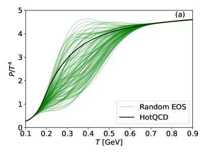
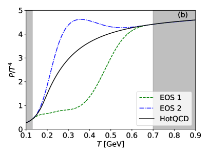
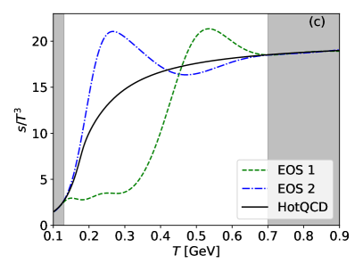
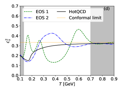
Figure 1a shows 100 randomly generated equations of state for their scaled pressure compared to the HotQCD + HRG EOS parameterized in Ref. Moreland and Soltz (2016) (the full black line). The GPR is allowed to vary freely at all temperature values in between the constraints. The randomly generated EOS sets show a wide spread around the lattice EOS in the unconstrained region and become more and more constrained towards the low and high-temperature region, as expected.
To explore the maximal effect of the EOS on the final state observables in relativistic heavy-ion collisions, we select two sets of EOS that envelope all the randomly generated EOS sets. To make the selection more efficient, we introduced anchor points at for EOS 1 and at for EOS 2. Their scaled pressures as functions of temperature are shown in Fig. 1b. Although EOS 2 shows non-monotonic dependence for its scaled pressure on temperature, its thermal pressure is a monotonic function of temperature.
Figure 1c shows the entropy density normalized by as a function of temperature. Compared to the lattice QCD EOS, the normalized entropy from the two sets of EOS at the extreme shows a non-monotonic dependence on temperature. Lastly, Figure 1d shows the square of the speed of sound for different EOS. Compared to the lattice QCD EOS, EOS 1 with smaller and near the phase cross-over region has a larger speed of sound in this temperature region. Because we impose the constraints on values of at high temperatures to those of the lattice QCD EOS, the speed of sound of the EOS oscillates around that of the lattice QCD EOS. The stiffer EOS near the phase cross-over region has a lower speed of sound at higher temperatures and vice versa.
III Deploy EOS to heavy-ion simulations
With the randomly generated equations of state, we invert and to tabulate thermal pressure as a function of energy density , which is then an input for hydrodynamic simulations to model the dynamical evolution of relativistic heavy-ion collisions.
III.1 Setup event-by-event simulations
To study the effects of different EOS on final state observables, we employ the iEBE-MUSIC framework Schenke et al. (2020a); Shen and Schenke (2022) to simulate event-by-event relativistic heavy-ion collisions.
In this work, we perform (2+1)D boost-invariant simulations with the IP-Glamsa + MUSIC + UrQMD model within the iEBE-MUSIC framework Schenke et al. (2020a). We set the model parameters based on a recent work Mäntysaari et al. (2024).
The initial states of the heavy-ion collisions are simulated event-by-event using the IP-Glasma model Schenke et al. (2012a); Mäntysaari et al. (2017). The Glasma pre-equilibrium evolution is propagated to , at which the system’s energy-momentum tensor is mapped to hydrodynamic fields using the Landau matching condition, Schenke et al. (2020b, a). After this time, the energy-momentum tensor is evolved using second-order relativistic viscous hydrodynamics based on the Denicol-Niemi-Molnar-Rischke (DNMR) theory Denicol et al. (2012). We incorporate the generated EOS from the GPR in solving the equation of motion of hydrodynamics in MUSIC Schenke et al. (2010, 2012b); Paquet et al. (2016). When the medium local energy density drops to the switching energy density GeV/fm3, the fluid cells on the constant energy surface are identified using the CORNELIUS algorithm Huovinen and Petersen (2012) and they are converted to particles according to the Cooper-Frye prescription Cooper and Frye (1974). Out-of-equilibrium () corrections to particle emission are considered using the Grad’s moment method Shen et al. (2016); Zhao et al. (2023). The thermally emitted hadrons are fed to a hadronic transport model, UrQMD Bass et al. (1998); Bleicher et al. (1999), to model the non-equilibrium hadronic scatterings and resonance decays in the dilute hadronic phase.
III.2 Second-order transport coefficients and causality constraints
The DNMR hydrodynamic theory introduces the second-order transport coefficients, such as the relaxation times for shear stress tensor and bulk viscous pressure. They are usually parameterized as functions of the specific shear and bulk viscosities Denicol et al. (2014). The parameterization for bulk viscous relaxation time is chosen to depend on Kanitscheider and Skenderis (2009); Rougemont et al. (2017); Denicol et al. (2014), where is the speed of sound squared from the EOS. Since we allow in our GPR generator, we need to modify the conventional parameterization of the to be well-defined when . The choices of these viscous relaxation times and other second-order transport coefficients are constrained by the causality conditions for relativistic viscous hydrodynamics Bemfica et al. (2021); Chiu and Shen (2021).
In this work, we assume the following parameterization for the viscous relaxation times,
| (12) | ||||
| (13) |
where and are constants, the second equality is only valid at zero chemical potential. Based on this parameterization, the linearized causality condition for second-order DNMR hydrodynamics can be written as Hiscock and Lindblom (1983)
| (14) |
In this work, we set and so that the constraints on the speed of sound squared in Eq. (14) translates to
| (15) |
Therefore, we can ensure the linearized causality condition for any EOS with smaller than .
According to Ref. Denicol et al. (2014), another second-order transport coefficient , which couples the bulk viscous pressure with the velocity shear tensor in the DNMR theory, has explicit dependence on the factor as
| (16) |
In this work, we set it to be the maximum value for any values of ,
| (17) |
III.3 EOS effects on final-state hadronic observables
We will now examine a few final-state observables and the effect of different EOS on them. In this work, we keep all the model parameters fixed in the simulations and only change the EOS to show its effects on final-state observables. We will perform a Bayesian inference study to constrain EOS together with all the other model parameters in future work.
Before we dive into the results, it is helpful for the understanding of the different behavior of the observables to note that the fireball spends most of its lifetime in the temperature region around MeV Paquet et al. (2016), where we observe a clear ordering in the speed of sound squared: . The flow development in the hydrodynamic phase is primarily sensitive to the values of in this temperature region.
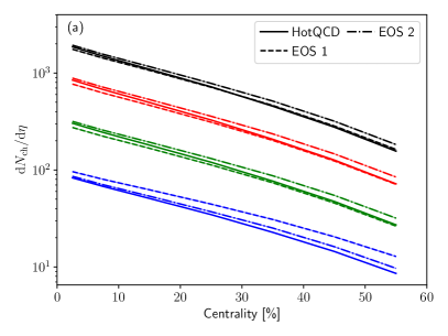
In Fig. 2, we show the EOS effects on a few -integrated observables as functions of collision centrality. The yields of charged hadron and identified particles in Fig. 2a show small sensitivity to the EOS. This is because most of the system’s entropy is produced in the IP-Glasma stage. The difference among the results from different EOS mainly comes from the different amounts of viscous entropy production during the hydrodynamic evolution. We observe that EOS 1 gives a larger to ratio than those from the other two EOS sets, indicating significant bulk viscous corrections at the particlization because it has a large near the cross-over region, which leads to fast expansion.
During the hydrodynamic evolution, the speed of sound in the EOS controls the size of local acceleration of the fluid velocity Heinz (2004),
| (18) |
The larger the , the stronger the acceleration from the same energy density gradients.
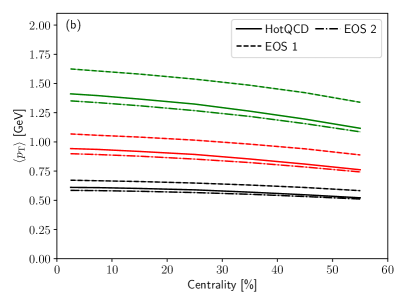
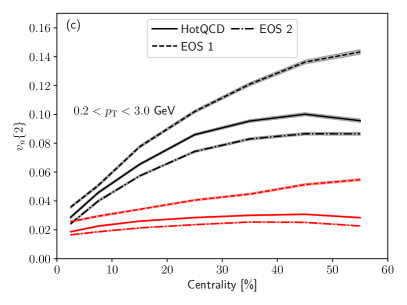
Figure 2b shows the identified particle average transverse momenta as functions of centrality from the three equations of state. Because final-state hadrons’ mean imprints the underlying hydrodynamic radial flow, hydrodynamic evolution with EOS 1 gives the largest mean for identified hadrons among the three. The ordering among the three EOS follows closely with their values in the temperature region between 150 and 250 MeV. The fast acceleration with the large speed of sound also results in larger anisotropic flow coefficients for charged hadrons, as shown in Fig. 2c. Again, we find the ordering of the results among the three equations of state is the same as their speed of sound near the cross-over region.
Since the speed of sound in equations of state is tightly correlated with the hydrodynamic flow event-by-event, we further study its effects on the fluctuation of hydrodynamic flow, which are imprinted in the charged hadron transverse momentum fluctuation. We compute the variance of the charged hadron fluctuation with
| (19) |
where the index sums over all charged hadrons in one subevent with and GeV and the index sums over all charged hadrons with and GeV in the same event. The fluctuation of each individual charged hadron is defined as with charged hadron averaged transverse momentum computed in the same kinematic cuts in the subevent. The denominator counts the number of particle pairs in the event. The averages over collision events.
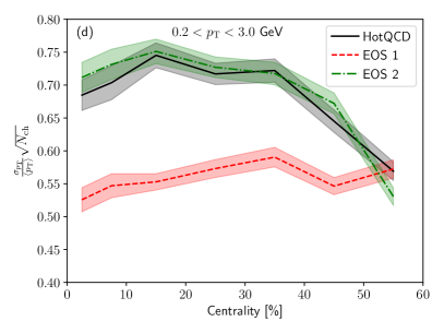
Figure 2d shows the normalized standard deviation of charged hadron scaled by as a function of centrality. Here, is the charged hadron multiplicity in GeV and . The factor scales out the trivial centrality dependence of fluctuations on finite numbers of charged hadrons Abelev et al. (2014); Schenke et al. (2020c). We observe that EOS 1 with a large speed of sound near the cross-over region results in small transverse momentum fluctuations. Furthermore, the centrality dependence of this scaled observable is also sensitive to the speed of sound in the EOS. The EOS with the low speed of sound in the temperature region MeV gives a decreasing trend of this scaled observable, while the results from EOS 1 are flat as a function of centrality.
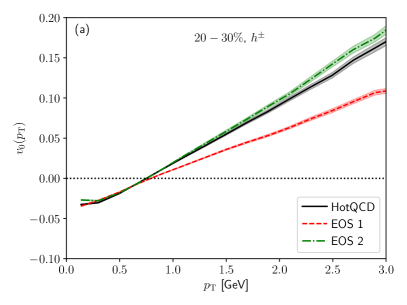
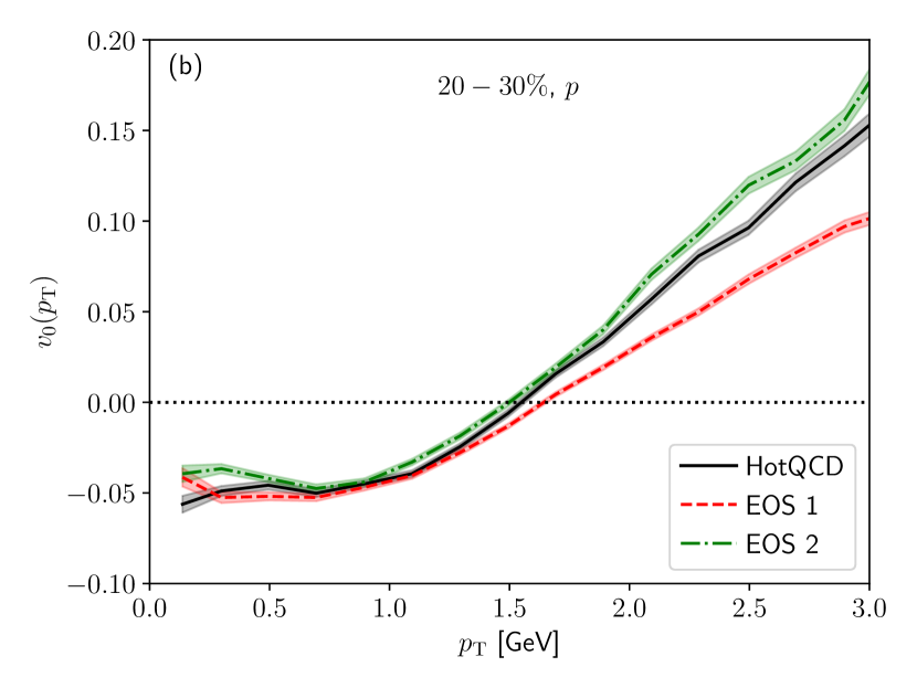
The charged hadron fluctuations can be further studied with the observables proposed in Ref. Schenke et al. (2020c). In a simple model Gardim et al. (2019); Schenke et al. (2020c), this observable can be interpreted as follows,
| (20) |
According to Eq. (20), crosses zero when and the slope of as a function of is related to the normalized standard deviation of the fluctuations. Figure 3 shows our simulation results of for charged hadrons in panel (a) and for protons in panel (b). We observe that the numerical results agree very well with the interpretations based on Eq. (20). Proton’s cross zero at GeV, inline with their mean values shown in Fig. 2b. Comparing from the three equations of state, we find that the ordering of the values when follows the mean ordering in Fig. 2b. Simulations with EOS 1 have a smaller slope of compared to those results from the other two EOS. It is consistent with the ordering of the fluctuations shown in Fig. 2d.
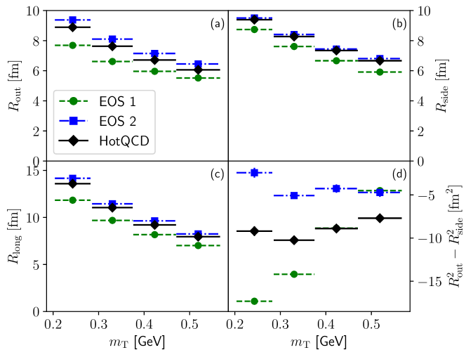
The two-particle Hanbury-Brown-Twiss (HBT) correlation is a sensitive probe for the speed of sound in the system Heinz (2004); Lisa et al. (2005); Pratt (2009); Pratt et al. (2015). For pairs of identical pions in the final state with momenta and , we define their pair momentum and momentum difference . Then, their HBT correlation can be computed as,
| (21) |
where the indices runs over all particle pairs within the transverse pair momentum bin and individual rapidity . The four-vector with the space-time position of the last interaction point of particle . The HBT correlation in Eq. (21) is usually expressed in the out-side-long coordinate system for . We perform a fit to the HBT correlation function using a 3D Gaussian Adamczyk et al. (2015),
| (22) |
from where we extract the HBT radii together with the cross terms .
Figure 4 shows the HBT radii , , , and as functions of pion’s transverse mass for Pb+Pb collisions at TeV. We find that the region of homogeneity in all three directions, measured by , , and , shows the same trends with decreasing values for equations of state with a high speed of sound near the cross-over region. Because the larger leads to faster hydrodynamic expansion in the transverse plane, the fireball has a shorter lifetime to grow its size when most of the pions are emitted, resulting in a smaller in panel (b) Pratt (2009). For and , they are sensitive to the time duration of the pion emission in addition to the spatial size of the homogeneous emission region in the fireball Wiedemann and Heinz (1999). The shorter fireball lifetime with EOS 1 results in smaller HBT radii in these two directions.
In Fig. 4d, we show the difference between and , which is sensitive to the averaged transverse flow velocity and lifetime of the fireball Wiedemann and Heinz (1999). With all three equations of state, in all bins. We can understand this trend based on a simplified Gaussian emission source Heinz (2004),
| (23) | ||||
| (24) |
where is the averaged fireball size squared in the side and out directions, respectively. For central Pb+Pb collisions, when . Our results in Fig. 4d indicate that the space-time correlation on the freeze-out surface is significantly positive in Pb+Pb collisions at TeV. With a larger average transverse velocity in simulations with EOS 1, the values of are more negative at small . We find at small shows strong sensitivity to the speed of sound in the equation of state. Furthermore, the dependence of is qualitatively different among the three equations of state.
Looking back at the EOS effects on final state observables in Figs. 2, 3, and 4, we find that all these hadronic observables are sensitive to the speed of sound near the crossover temperature region, GeV. The EOS 2 has the highest speed of sound when GeV; however because only a small fraction of fluid cells probes this temperature region such that hadronic observables are not sensitive to them.
III.4 EOS effects on electromagnetic radiation
Electromagnetic probes, such as thermal photons and dileptons, are sensitive to the local temperature and flow field at their emission points. They carry valuable information about early-time dynamics of heavy-ion collisions, complementary to final-state hadronic observables Shen (2016); Gale et al. (2019, 2022); Shen et al. (2024a); Churchill et al. (2024); Wu et al. (2024).
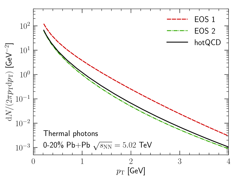
Figure 5 shows the thermal photon spectra emitted from QGP and hot hadron gas phases in Pb+Pb collisions with the three different equations of state. They are computed by convoluting the thermal photon emission rates with the fireballs’ dynamical evolution profiles event by event. We used the leading-order QGP photon emission rates Arnold et al. (2001) for fluid cells with temperatures above 180 MeV and hadronic gas photon emission rates Turbide et al. (2004); Heffernan et al. (2015) for those fluid cells with temperatures between 120-180 MeV. The leading order out-of-equilibrium corrections to thermal photon emission rates are included for the available photon emission channels Shen et al. (2015); Paquet et al. (2016); Hauksson et al. (2017).
We observe that the simulations with EOS 1 result in a factor of 3 more thermal photons than those from simulations with the other two equations of state. The EOS 1 has the smallest values among the three equations of state, as shown in Fig. 1, which leads to the highest local temperature for fluid cells at a given energy density. Then, the higher temperature in EOS 1 results in more thermal photon radiation. Unlike the hadronic observables, which are sensitive to the time-integrated EOS effects on hydrodynamic flow, the thermal photon spectra show direct sensitivity to the temperature profile of the collisions given by the equation of state. Figure 5 demonstrates that the yields of thermal photon radiation are a direct probe to the thermodynamic properties of the hot QCD matter.
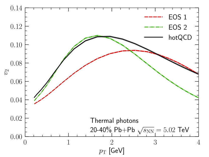
The fireball’s flow profile can be probed by the elliptic flow coefficients of thermal photons, as shown in Fig. 6. Different from the hadrons’ elliptic flow, thermal photons with high transverse momenta are mostly emitted during the early phase of the evolution at which the hydrodynamic flow has not fully developed. It results in the rise and fall structure in the -dependence of thermal photon elliptic flow coefficients. We find that the simulations with EOS 1 have the lowest for GeV among the three equations of state. The trend in thermal photon is the exact opposite of the ordering in charged hadrons shown in Fig. 2c. Because EOS 1 has the highest temperatures at a given energy density compared to those from the other two equations of state, the thermal photon radiation from EOS 1 is dominated by the high-temperature phase where the hydrodynamic anisotropic flow has not fully developed. There are more photon emissions from the hot hadron gas phase with EOS 2 and the hot QCD EOS, which increases the thermal photon in the low region.
IV Conclusion
In this paper, we employ Gaussian Process regression as a generative model to produce random smooth cross-over type QCD equations of state. This model allows us to impose desired physics constraints from thermodynamics and causality and provides enough variations in the allowed phase space. We demonstrate the results at zero baryon density, where the thermal pressure is only a function of temperature . Our formulation can easily be extended to higher dimensions, including dependencies on conserved charges like baryon, strangeness, and electric charges.
We deploy this EOS generator to the iEBE-MUSIC framework and perform event-by-event simulations for Pb+Pb collisions at TeV to explore the effects of EOS on final-state observables. We find that most of the hadronic observables are sensitive to the values of the speed of sound near the cross-over region between the hadron gas and QGP phases, where GeV. A high speed of sound in the equation of state results in a large acceleration rate from the local energy density gradients and leads to the fast development of the radial and anisotropic flow during the hydrodynamic phase. Hadron’s averaged transverse momenta, the variance of fluctuations, and anisotropic flow coefficients show strong responses to the variations in EOS. The HBT radii of identical pion pairs are also sensitive observables for probing the speed of sound in the equation of state. Finally, we study the effects of the EOS on electromagnetic radiation. We find that the yields of thermal photons are strongly affected by the temperature profile encoded in the equation of state. It demonstrated the tomographic nature of thermal photons to probe the thermodynamic properties of hot QCD matter. The elliptic flow of thermal photons is sensitive to the relative photon emission at different temperatures and times, providing complementary information about the hydrodynamic flow development to those inferred from hadrons’ anisotropic flow coefficients.
The observed strong sensitivities in final-state observables to the variations in the equation of state pave a good starting point for a systematic Bayesian inference study on constraining the QCD EOS using experimental measurements from relativistic heavy-ion collisions. It would be interesting to compare the results from such a data-driven approach at zero baryon density with the ones from the first-principle calculation, which we will pursue as future work. We also plan to extend the current generative model to finite baryon density and carry out dedicated Bayesian inference studies to constrain the behavior of QCD EOS at large baryon density with measurements in the RHIC Beam Energy Scan program.
The code developed for this work is open source and can be downloaded from Gong et al. (2024).
Acknowledgements.
This work is supported in part by the U.S. Department of Energy, Office of Science, Office of Nuclear Physics, under DOE Award No. DE-SC0021969 and DE-SC0024232. H. R. was supported in part by the National Science Foundation (NSF) within the framework of the JETSCAPE collaboration (OAC-2004571). C.S. acknowledges a DOE Office of Science Early Career Award. This research was done using computational resources provided by the Open Science Grid (OSG) et al. (2007); Sfiligoi et al. (2009), which is supported by the National Science Foundation award #2030508 and #1836650.References
- Pratt et al. (2015) Scott Pratt, Evan Sangaline, Paul Sorensen, and Hui Wang, “Constraining the Eq. of State of Super-Hadronic Matter from Heavy-Ion Collisions,” Phys. Rev. Lett. 114, 202301 (2015), arXiv:1501.04042 [nucl-th] .
- Busza et al. (2018) Wit Busza, Krishna Rajagopal, and Wilke van der Schee, “Heavy Ion Collisions: The Big Picture, and the Big Questions,” Ann. Rev. Nucl. Part. Sci. 68, 339–376 (2018), arXiv:1802.04801 [hep-ph] .
- Shen and Yan (2020) Chun Shen and Li Yan, “Recent development of hydrodynamic modeling in heavy-ion collisions,” Nucl. Sci. Tech. 31, 122 (2020), arXiv:2010.12377 [nucl-th] .
- An et al. (2022) Xin An et al., “The BEST framework for the search for the QCD critical point and the chiral magnetic effect,” Nucl. Phys. A 1017, 122343 (2022), arXiv:2108.13867 [nucl-th] .
- Monnai et al. (2021) Akihiko Monnai, Björn Schenke, and Chun Shen, “QCD Equation of State at Finite Chemical Potentials for Relativistic Nuclear Collisions,” Int. J. Mod. Phys. A 36, 2130007 (2021), arXiv:2101.11591 [nucl-th] .
- Almaalol et al. (2022) D. Almaalol et al., “QCD Phase Structure and Interactions at High Baryon Density: Continuation of BES Physics Program with CBM at FAIR,” (2022), arXiv:2209.05009 [nucl-ex] .
- Sorensen et al. (2024) Agnieszka Sorensen et al., “Dense nuclear matter equation of state from heavy-ion collisions,” Prog. Part. Nucl. Phys. 134, 104080 (2024), arXiv:2301.13253 [nucl-th] .
- Achenbach et al. (2024) P. Achenbach et al., “The present and future of QCD,” Nucl. Phys. A 1047, 122874 (2024), arXiv:2303.02579 [hep-ph] .
- Arslandok et al. (2023) M. Arslandok et al., “Hot QCD White Paper,” (2023), arXiv:2303.17254 [nucl-ex] .
- Du et al. (2024a) Lipei Du, Agnieszka Sorensen, and Mikhail Stephanov, “The QCD phase diagram and Beam Energy Scan physics: a theory overview,” Int. J. Mod. Phys. E 33, 2430008 (2024a), arXiv:2402.10183 [nucl-th] .
- Borsanyi et al. (2014) Szabocls Borsanyi, Zoltan Fodor, Christian Hoelbling, Sandor D. Katz, Stefan Krieg, and Kalman K. Szabo, “Full result for the QCD equation of state with 2+1 flavors,” Phys. Lett. B 730, 99–104 (2014), arXiv:1309.5258 [hep-lat] .
- Bazavov et al. (2014) A. Bazavov et al. (HotQCD), “Equation of state in ( 2+1 )-flavor QCD,” Phys. Rev. D 90, 094503 (2014), arXiv:1407.6387 [hep-lat] .
- Shen et al. (2016) Chun Shen, Zhi Qiu, Huichao Song, Jonah Bernhard, Steffen Bass, and Ulrich Heinz, “The iEBE-VISHNU code package for relativistic heavy-ion collisions,” Comput. Phys. Commun. 199, 61–85 (2016), arXiv:1409.8164 [nucl-th] .
- Giacalone et al. (2018) Giuliano Giacalone, Jacquelyn Noronha-Hostler, Matthew Luzum, and Jean-Yves Ollitrault, “Hydrodynamic predictions for 5.44 TeV Xe+Xe collisions,” Phys. Rev. C 97, 034904 (2018), arXiv:1711.08499 [nucl-th] .
- Putschke et al. (2019) J. H. Putschke et al., “The JETSCAPE framework,” (2019), arXiv:1903.07706 [nucl-th] .
- Schenke et al. (2020a) Bjoern Schenke, Chun Shen, and Prithwish Tribedy, “Running the gamut of high energy nuclear collisions,” Phys. Rev. C 102, 044905 (2020a), arXiv:2005.14682 [nucl-th] .
- Nijs et al. (2021) Govert Nijs, Wilke van der Schee, Umut Gürsoy, and Raimond Snellings, “Transverse Momentum Differential Global Analysis of Heavy-Ion Collisions,” Phys. Rev. Lett. 126, 202301 (2021), arXiv:2010.15130 [nucl-th] .
- Hirvonen et al. (2024) Henry Hirvonen, Mikko Kuha, Jussi Auvinen, Kari J. Eskola, Yuuka Kanakubo, and Harri Niemi, “Effects of saturation and fluctuating hotspots for flow observables in ultrarelativistic heavy-ion collisions,” Phys. Rev. C 110, 034911 (2024), arXiv:2407.01338 [hep-ph] .
- Fodor and Katz (2004) Z. Fodor and S. D. Katz, “Critical point of QCD at finite T and mu, lattice results for physical quark masses,” JHEP 04, 050 (2004), arXiv:hep-lat/0402006 .
- Gavai and Gupta (2008) R. V. Gavai and Sourendu Gupta, “QCD at finite chemical potential with six time slices,” Phys. Rev. D 78, 114503 (2008), arXiv:0806.2233 [hep-lat] .
- Bazavov et al. (2017) A. Bazavov et al., “The QCD Equation of State to from Lattice QCD,” Phys. Rev. D 95, 054504 (2017), arXiv:1701.04325 [hep-lat] .
- Giordano et al. (2020) Matteo Giordano, Kornel Kapas, Sandor D. Katz, Daniel Nogradi, and Attila Pasztor, “New approach to lattice QCD at finite density; results for the critical end point on coarse lattices,” JHEP 05, 088 (2020), arXiv:2004.10800 [hep-lat] .
- Borsányi et al. (2021) S. Borsányi, Z. Fodor, J. N. Guenther, R. Kara, S. D. Katz, P. Parotto, A. Pásztor, C. Ratti, and K. K. Szabó, “Lattice QCD equation of state at finite chemical potential from an alternative expansion scheme,” Phys. Rev. Lett. 126, 232001 (2021), arXiv:2102.06660 [hep-lat] .
- Ratti (2018) Claudia Ratti, “Lattice QCD and heavy ion collisions: a review of recent progress,” Rept. Prog. Phys. 81, 084301 (2018), arXiv:1804.07810 [hep-lat] .
- Caines (2009) Helen Caines (STAR), “The RHIC Beam Energy Scan: STAR’S Perspective,” in 44th Rencontres de Moriond on QCD and High Energy Interactions (2009) pp. 375–378, arXiv:0906.0305 [nucl-ex] .
- Mohanty (2011) Bedangadas Mohanty (STAR), “STAR experiment results from the beam energy scan program at RHIC,” J. Phys. G 38, 124023 (2011), arXiv:1106.5902 [nucl-ex] .
- Mitchell (2013) Jeffery T. Mitchell (PHENIX), “The RHIC Beam Energy Scan Program: Results from the PHENIX Experiment,” Nucl. Phys. A 904-905, 903c–906c (2013), arXiv:1211.6139 [nucl-ex] .
- Odyniec (2015) Grazyna Odyniec, “Future of the beam energy scan program at RHIC,” EPJ Web Conf. 95, 03027 (2015).
- Aggarwal et al. (2010) M. M. Aggarwal et al. (STAR), “An Experimental Exploration of the QCD Phase Diagram: The Search for the Critical Point and the Onset of De-confinement,” (2010), arXiv:1007.2613 [nucl-ex] .
- Luo and Xu (2017) Xiaofeng Luo and Nu Xu, “Search for the QCD Critical Point with Fluctuations of Conserved Quantities in Relativistic Heavy-Ion Collisions at RHIC : An Overview,” Nucl. Sci. Tech. 28, 112 (2017), arXiv:1701.02105 [nucl-ex] .
- Bzdak et al. (2020) Adam Bzdak, Shinichi Esumi, Volker Koch, Jinfeng Liao, Mikhail Stephanov, and Nu Xu, “Mapping the Phases of Quantum Chromodynamics with Beam Energy Scan,” Phys. Rept. 853, 1–87 (2020), arXiv:1906.00936 [nucl-th] .
- Auvinen et al. (2018) Jussi Auvinen, Jonah E. Bernhard, Steffen A. Bass, and Iurii Karpenko, “Investigating the collision energy dependence of /s in the beam energy scan at the BNL Relativistic Heavy Ion Collider using Bayesian statistics,” Phys. Rev. C 97, 044905 (2018), arXiv:1706.03666 [hep-ph] .
- Sun and Ko (2023) Kai-Jia Sun and Che Ming Ko, “Event-by-event antideuteron multiplicity fluctuation in Pb+Pb collisions at sNN=5.02 TeV,” Phys. Lett. B 840, 137864 (2023), arXiv:2204.10879 [nucl-th] .
- Shen and Schenke (2022) Chun Shen and Björn Schenke, “Longitudinal dynamics and particle production in relativistic nuclear collisions,” Phys. Rev. C 105, 064905 (2022), arXiv:2203.04685 [nucl-th] .
- Shen et al. (2024a) Chun Shen, Abel Noble, Jean-François Paquet, Björn Schenke, and Charles Gale, “Illuminating early-stage dynamics of heavy-ion collisions through photons at RHIC BES energies,” PoS HardProbes2023, 042 (2024a), arXiv:2307.08498 [nucl-th] .
- Shen et al. (2024b) Chun Shen, Björn Schenke, and Wenbin Zhao, “Viscosities of the Baryon-Rich Quark-Gluon Plasma from Beam Energy Scan Data,” Phys. Rev. Lett. 132, 072301 (2024b), arXiv:2310.10787 [nucl-th] .
- Jiang et al. (2023) Ze-Fang Jiang, Xiang-Yu Wu, Hua-Qing Yu, Shan-Shan Cao, and Ben-Wei Zhang, “The direct flow of charged particles and the global polarization of hyperons in 200 AGeV Au+Au collisions at RHIC,” Acta Phys. Sin. 72, 072504 (2023).
- Du et al. (2024b) Lipei Du, Han Gao, Sangyong Jeon, and Charles Gale, “Rapidity scan with multistage hydrodynamic and statistical thermal models,” Phys. Rev. C 109, 014907 (2024b), arXiv:2302.13852 [nucl-th] .
- Du et al. (2024c) Lipei Du, Chun Shen, Sangyong Jeon, and Charles Gale, “Constraints on initial baryon stopping and equation of state from directed flow,” EPJ Web Conf. 296, 05011 (2024c), arXiv:2312.06468 [nucl-th] .
- Shen et al. (2024c) Chun Shen, Björn Schenke, and Wenbin Zhao, “The effects of pseudorapidity-dependent observables on (3+1)D Bayesian Inference of relativistic heavy-ion collisions,” EPJ Web Conf. 296, 14001 (2024c), arXiv:2312.09325 [nucl-th] .
- Plumberg et al. (2024) Christopher Plumberg et al., “BSQ Conserved Charges in Relativistic Viscous Hydrodynamics solved with Smoothed Particle Hydrodynamics,” (2024), arXiv:2405.09648 [nucl-th] .
- Pihan et al. (2024) Gregoire Pihan, Akihiko Monnai, Björn Schenke, and Chun Shen, “Unveiling baryon charge carriers through charge stopping in isobar collisions,” (2024), arXiv:2405.19439 [nucl-th] .
- Monnai et al. (2024) Akihiko Monnai, Grégoire Pihan, Björn Schenke, and Chun Shen, “Four-dimensional QCD equation of state with multiple chemical potentials,” Phys. Rev. C 110, 044905 (2024), arXiv:2406.11610 [nucl-th] .
- Jahan et al. (2024) Syed Afrid Jahan, Hendrik Roch, and Chun Shen, “Bayesian analysis of (3+1)D relativistic nuclear dynamics with the RHIC beam energy scan data,” (2024), arXiv:2408.00537 [nucl-th] .
- Monnai et al. (2019) Akihiko Monnai, Björn Schenke, and Chun Shen, “Equation of state at finite densities for QCD matter in nuclear collisions,” Phys. Rev. C 100, 024907 (2019), arXiv:1902.05095 [nucl-th] .
- Noronha-Hostler et al. (2019) J. Noronha-Hostler, P. Parotto, C. Ratti, and J. M. Stafford, “Lattice-based equation of state at finite baryon number, electric charge and strangeness chemical potentials,” Phys. Rev. C 100, 064910 (2019), arXiv:1902.06723 [hep-ph] .
- Fotakis et al. (2020) Jan A. Fotakis, Moritz Greif, Carsten Greiner, Gabriel S. Denicol, and Harri Niemi, “Diffusion processes involving multiple conserved charges: A study from kinetic theory and implications to the fluid-dynamical modeling of heavy ion collisions,” Phys. Rev. D 101, 076007 (2020), arXiv:1912.09103 [hep-ph] .
- Karthein et al. (2021) J. M. Karthein, D. Mroczek, A. R. Nava Acuna, J. Noronha-Hostler, P. Parotto, D. R. P. Price, and C. Ratti, “Strangeness-neutral equation of state for QCD with a critical point,” Eur. Phys. J. Plus 136, 621 (2021), arXiv:2103.08146 [hep-ph] .
- Mondal et al. (2022) Sourav Mondal, Swagato Mukherjee, and Prasad Hegde, “Lattice QCD Equation of State for Nonvanishing Chemical Potential by Resumming Taylor Expansions,” Phys. Rev. Lett. 128, 022001 (2022), arXiv:2106.03165 [hep-lat] .
- Novak et al. (2014) John Novak, Kevin Novak, Scott Pratt, Joshua Vredevoogd, Chris Coleman-Smith, and Robert Wolpert, “Determining Fundamental Properties of Matter Created in Ultrarelativistic Heavy-Ion Collisions,” Phys. Rev. C 89, 034917 (2014), arXiv:1303.5769 [nucl-th] .
- Bernhard et al. (2019) Jonah E. Bernhard, J. Scott Moreland, and Steffen A. Bass, “Bayesian estimation of the specific shear and bulk viscosity of quark–gluon plasma,” Nature Phys. 15, 1113–1117 (2019).
- Everett et al. (2021) D. Everett et al. (JETSCAPE), “Multisystem Bayesian constraints on the transport coefficients of QCD matter,” Phys. Rev. C 103, 054904 (2021), arXiv:2011.01430 [hep-ph] .
- Giacalone et al. (2023) Giuliano Giacalone, Govert Nijs, and Wilke van der Schee, “Determination of the Neutron Skin of Pb208 from Ultrarelativistic Nuclear Collisions,” Phys. Rev. Lett. 131, 202302 (2023), arXiv:2305.00015 [nucl-th] .
- Landry and Essick (2019) Philippe Landry and Reed Essick, “Nonparametric inference of the neutron star equation of state from gravitational wave observations,” Phys. Rev. D 99, 084049 (2019), arXiv:1811.12529 [gr-qc] .
- Mroczek et al. (2023) Debora Mroczek, M. Coleman Miller, Jacquelyn Noronha-Hostler, and Nicolas Yunes, “Nontrivial features in the speed of sound inside neutron stars,” (2023), arXiv:2309.02345 [astro-ph.HE] .
- Williams and Rasmussen (2006) Christopher KI Williams and Carl Edward Rasmussen, Gaussian processes for machine learning, Vol. 2 (MIT press Cambridge, MA, 2006).
- Hippert et al. (2024) Mauricio Hippert, Jorge Noronha, and Paul Romatschke, “Upper Bound on the Speed of Sound in Nuclear Matter from Transport,” (2024), arXiv:2402.14085 [nucl-th] .
- Moore (2024) Guy D. Moore, “Hydrodynamics as vs → c,” JHEP 06, 171 (2024), arXiv:2404.01968 [hep-ph] .
- Moreland and Soltz (2016) J. Scott Moreland and Ron A. Soltz, “Hydrodynamic simulations of relativistic heavy-ion collisions with different lattice quantum chromodynamics calculations of the equation of state,” Phys. Rev. C 93, 044913 (2016), arXiv:1512.02189 [nucl-th] .
- Mäntysaari et al. (2024) Heikki Mäntysaari, Björn Schenke, Chun Shen, and Wenbin Zhao, “Probing Nuclear Structure of Heavy Ions at the Large Hadron Collider,” (2024), arXiv:2409.19064 [nucl-th] .
- Schenke et al. (2012a) Bjoern Schenke, Prithwish Tribedy, and Raju Venugopalan, “Fluctuating Glasma initial conditions and flow in heavy ion collisions,” Phys. Rev. Lett. 108, 252301 (2012a), arXiv:1202.6646 [nucl-th] .
- Mäntysaari et al. (2017) Heikki Mäntysaari, Björn Schenke, Chun Shen, and Prithwish Tribedy, “Imprints of fluctuating proton shapes on flow in proton-lead collisions at the LHC,” Phys. Lett. B 772, 681–686 (2017), arXiv:1705.03177 [nucl-th] .
- Schenke et al. (2020b) Bjoern Schenke, Chun Shen, and Prithwish Tribedy, “Hybrid Color Glass Condensate and hydrodynamic description of the Relativistic Heavy Ion Collider small system scan,” Phys. Lett. B 803, 135322 (2020b), arXiv:1908.06212 [nucl-th] .
- Denicol et al. (2012) G. S. Denicol, H. Niemi, E. Molnar, and D. H. Rischke, “Derivation of transient relativistic fluid dynamics from the Boltzmann equation,” Phys. Rev. D 85, 114047 (2012), [Erratum: Phys.Rev.D 91, 039902 (2015)], arXiv:1202.4551 [nucl-th] .
- Schenke et al. (2010) Bjoern Schenke, Sangyong Jeon, and Charles Gale, “(3+1)D hydrodynamic simulation of relativistic heavy-ion collisions,” Phys. Rev. C 82, 014903 (2010), arXiv:1004.1408 [hep-ph] .
- Schenke et al. (2012b) Bjorn Schenke, Sangyong Jeon, and Charles Gale, “Higher flow harmonics from (3+1)D event-by-event viscous hydrodynamics,” Phys. Rev. C 85, 024901 (2012b), arXiv:1109.6289 [hep-ph] .
- Paquet et al. (2016) Jean-François Paquet, Chun Shen, Gabriel S. Denicol, Matthew Luzum, Björn Schenke, Sangyong Jeon, and Charles Gale, “Production of photons in relativistic heavy-ion collisions,” Phys. Rev. C 93, 044906 (2016), arXiv:1509.06738 [hep-ph] .
- Huovinen and Petersen (2012) Pasi Huovinen and Hannah Petersen, “Particlization in hybrid models,” Eur. Phys. J. A 48, 171 (2012), arXiv:1206.3371 [nucl-th] .
- Cooper and Frye (1974) Fred Cooper and Graham Frye, “Comment on the Single Particle Distribution in the Hydrodynamic and Statistical Thermodynamic Models of Multiparticle Production,” Phys. Rev. D 10, 186 (1974).
- Zhao et al. (2023) Wenbin Zhao, Sangwook Ryu, Chun Shen, and Björn Schenke, “3D structure of anisotropic flow in small collision systems at energies available at the BNL Relativistic Heavy Ion Collider,” Phys. Rev. C 107, 014904 (2023), arXiv:2211.16376 [nucl-th] .
- Bass et al. (1998) S. A. Bass et al., “Microscopic models for ultrarelativistic heavy ion collisions,” Prog. Part. Nucl. Phys. 41, 255–369 (1998), arXiv:nucl-th/9803035 .
- Bleicher et al. (1999) M. Bleicher et al., “Relativistic hadron hadron collisions in the ultrarelativistic quantum molecular dynamics model,” J. Phys. G 25, 1859–1896 (1999), arXiv:hep-ph/9909407 .
- Denicol et al. (2014) G. S. Denicol, S. Jeon, and C. Gale, “Transport Coefficients of Bulk Viscous Pressure in the 14-moment approximation,” Phys. Rev. C 90, 024912 (2014), arXiv:1403.0962 [nucl-th] .
- Kanitscheider and Skenderis (2009) Ingmar Kanitscheider and Kostas Skenderis, “Universal hydrodynamics of non-conformal branes,” JHEP 04, 062 (2009), arXiv:0901.1487 [hep-th] .
- Rougemont et al. (2017) Romulo Rougemont, Renato Critelli, Jacquelyn Noronha-Hostler, Jorge Noronha, and Claudia Ratti, “Dynamical versus equilibrium properties of the QCD phase transition: A holographic perspective,” Phys. Rev. D 96, 014032 (2017), arXiv:1704.05558 [hep-ph] .
- Bemfica et al. (2021) Fábio S. Bemfica, Marcelo M. Disconzi, Vu Hoang, Jorge Noronha, and Maria Radosz, “Nonlinear Constraints on Relativistic Fluids Far from Equilibrium,” Phys. Rev. Lett. 126, 222301 (2021), arXiv:2005.11632 [hep-th] .
- Chiu and Shen (2021) Cheng Chiu and Chun Shen, “Exploring theoretical uncertainties in the hydrodynamic description of relativistic heavy-ion collisions,” Phys. Rev. C 103, 064901 (2021), arXiv:2103.09848 [nucl-th] .
- Hiscock and Lindblom (1983) W. A. Hiscock and L. Lindblom, “Stability and causality in dissipative relativistic fluids,” Annals Phys. 151, 466–496 (1983).
- Heinz (2004) Ulrich W. Heinz, “Concepts of heavy ion physics,” in 2nd CERN-CLAF School of High Energy Physics (2004) pp. 165–238, arXiv:hep-ph/0407360 .
- Abelev et al. (2014) Betty Bezverkhny Abelev et al. (ALICE), “Event-by-event mean fluctuations in pp and Pb-Pb collisions at the LHC,” Eur. Phys. J. C 74, 3077 (2014), arXiv:1407.5530 [nucl-ex] .
- Schenke et al. (2020c) Björn Schenke, Chun Shen, and Derek Teaney, “Transverse momentum fluctuations and their correlation with elliptic flow in nuclear collision,” Phys. Rev. C 102, 034905 (2020c), arXiv:2004.00690 [nucl-th] .
- Gardim et al. (2019) Fernando G. Gardim, Frédérique Grassi, Pedro Ishida, Matthew Luzum, and Jean-Yves Ollitrault, “-dependent particle number fluctuations from principal-component analyses in hydrodynamic simulations of heavy-ion collisions,” Phys. Rev. C 100, 054905 (2019), arXiv:1906.03045 [nucl-th] .
- Lisa et al. (2005) Michael Annan Lisa, Scott Pratt, Ron Soltz, and Urs Wiedemann, “Femtoscopy in relativistic heavy ion collisions,” Ann. Rev. Nucl. Part. Sci. 55, 357–402 (2005), arXiv:nucl-ex/0505014 .
- Pratt (2009) Scott Pratt, “Resolving the HBT Puzzle in Relativistic Heavy Ion Collision,” Phys. Rev. Lett. 102, 232301 (2009), arXiv:0811.3363 [nucl-th] .
- Adamczyk et al. (2015) L. Adamczyk et al. (STAR), “Beam-energy-dependent two-pion interferometry and the freeze-out eccentricity of pions measured in heavy ion collisions at the STAR detector,” Phys. Rev. C 92, 014904 (2015), arXiv:1403.4972 [nucl-ex] .
- Wiedemann and Heinz (1999) Urs Achim Wiedemann and Ulrich W. Heinz, “Particle interferometry for relativistic heavy ion collisions,” Phys. Rept. 319, 145–230 (1999), arXiv:nucl-th/9901094 .
- Shen (2016) Chun Shen, “Electromagnetic Radiation from QCD Matter: Theory Overview,” Nucl. Phys. A 956, 184–191 (2016), arXiv:1601.02563 [nucl-th] .
- Gale et al. (2019) Charles Gale, Sangyong Jeon, Scott McDonald, Jean-François Paquet, and Chun Shen, “Photon radiation from heavy-ion collisions in the GeV regime,” Nucl. Phys. A 982, 767–770 (2019), arXiv:1807.09326 [nucl-th] .
- Gale et al. (2022) Charles Gale, Jean-François Paquet, Björn Schenke, and Chun Shen, “Multimessenger heavy-ion collision physics,” Phys. Rev. C 105, 014909 (2022), arXiv:2106.11216 [nucl-th] .
- Churchill et al. (2024) Jessica Churchill, Lipei Du, Charles Gale, Greg Jackson, and Sangyong Jeon, “Virtual Photons Shed Light on the Early Temperature of Dense QCD Matter,” Phys. Rev. Lett. 132, 172301 (2024), arXiv:2311.06951 [nucl-th] .
- Wu et al. (2024) Xiang-Yu Wu, Lipei Du, Charles Gale, and Sangyong Jeon, “Probing the equilibration of the QCD matter created in heavy-ion collisions with dileptons,” (2024), arXiv:2407.04156 [nucl-th] .
- Arnold et al. (2001) Peter Brockway Arnold, Guy D. Moore, and Laurence G. Yaffe, “Photon emission from quark gluon plasma: Complete leading order results,” JHEP 12, 009 (2001), arXiv:hep-ph/0111107 .
- Turbide et al. (2004) Simon Turbide, Ralf Rapp, and Charles Gale, “Hadronic production of thermal photons,” Phys. Rev. C 69, 014903 (2004), arXiv:hep-ph/0308085 .
- Heffernan et al. (2015) Matthew Heffernan, Paul Hohler, and Ralf Rapp, “Universal Parametrization of Thermal Photon Rates in Hadronic Matter,” Phys. Rev. C 91, 027902 (2015), arXiv:1411.7012 [hep-ph] .
- Shen et al. (2015) Chun Shen, Jean-Francois Paquet, Ulrich Heinz, and Charles Gale, “Photon Emission from a Momentum Anisotropic Quark-Gluon Plasma,” Phys. Rev. C 91, 014908 (2015), arXiv:1410.3404 [nucl-th] .
- Hauksson et al. (2017) Sigtryggur Hauksson, Chun Shen, Sangyong Jeon, and Charles Gale, “Bulk viscous corrections to photon production in the quark–gluon plasma,” Nucl. Part. Phys. Proc. 289-290, 169–172 (2017), arXiv:1612.05517 [nucl-th] .
- Gong et al. (2024) Jiaxuan Gong, Hendrik Roch, and Chun Shen, “Hendrik1704/gp_eos_generator: v1.0.0,” (2024).
- et al. (2007) Ruth Pordes et al., “The open science grid,” Journal of Physics: Conference Series 78, 012057 (2007).
- Sfiligoi et al. (2009) Igor Sfiligoi, Daniel C. Bradley, Burt Holzman, Parag Mhashilkar, Sanjay Padhi, and Frank Wurthwein, “The pilot way to grid resources using glideinwms,” in 2009 WRI World Congress on Computer Science and Information Engineering, Vol. 2 (2009) pp. 428–432.