Averaging principle for multiscale controlled jump diffusions and associated nonlocal HJB equations

Abstract

This paper studies the averaging principle of a class of two-time scale stochastic control systems with $\alpha$-stable noise. The associated singular perturbations problem for nonlocal Hamilton-Jacobi-Bellman (HJB) equations is also considered. We construct the effective stochastic control problem and the associated effective HJB equation for the original multiscale stochastic control problem by averaging over the ergodic measure of the fast component. We prove the convergence of the value function using two methods. With the probabilistic method, we show that the value function of the original multiscale stochastic control system converges to the value function of the effective stochastic control system by proving the weak averaging principle of the controlled jump diffusions. Using the PDE method, we study the value function as the viscosity solution of the associated nonlocal HJB equation with singular perturbations. We then prove the convergence using the perturbed test function method.

Keywords and Phrases: stochastic optimal control, singular perturbations, nonlocal Poisson equation, tightness, nonlocal HJB equation.

1 Introduction

In this paper, we consider the controlled jump diffusions described by the slow-fast stochastic differential equation (SDE) with Lévy noises

$$\left\{\begin{aligned} d{X^{\epsilon}_{s}}&=b({X^{\epsilon}_{s}},{Y^{\epsilon}_{s}},v_{s})ds+d\textbf{L}_{s}^{{\alpha}_{1}},\quad X^{\epsilon}_{t}=x,\\ d{Y^{\epsilon}_{s}}&=\frac{1}{\epsilon}c({X^{\epsilon}_{s}},Y^{\epsilon}_{s})ds+\epsilon^{-\frac{1}{\alpha_{2}}}d\textbf{L}_{s}^{{\alpha_{2}}},\quad Y^{\epsilon}_{t}=y,\\ \end{aligned}\right.$$ (1.1)

where $0\leq t\leq s$, $X_{s}^{\epsilon}\in\mathbb{R}^{n}$ is the slow component, $Y_{s}^{\epsilon}\in\mathbb{R}^{m}$ the fast component, $\textbf{L}^{{\alpha_{i}}}_{s},i=1,2$ are independent symmetric $\alpha_{i}$-stable ($1<\alpha_{i}<2$) Lévy processes, $v_{s}$ is the control taking values in a given processes $\mathcal{U}$ with values in a given closed convex subset set $U\subseteq\mathbb{R}^{r}$, drifts $b,c$ are Borel measurable functions on $\mathbb{R}^{n}\times\mathbb{R}^{m}$ which satisfies some conditions implying the wellposedness of $(X_{s}^{\epsilon},Y_{s}^{\epsilon})$ and the ergodicity of $Y^{\epsilon}$. The precise assumptions are detailed in Section 2. As the time scale $\epsilon\to 0$, the fast components can be viewed as singular perturbations to the original system.

We carry our analysis of the multiscale scale stochastic control problem with the cost-functional or payoff functional

$$J^{\epsilon}(v,x,y,t)=\mathbb{E}\left[-\int^{T}_{t}e^{\lambda(s-T)}L\left(X^{\epsilon}_{s},Y^{\epsilon}_{s},v_{s}\right)ds+e^{\lambda(t-T)}g\left(X^{\epsilon}_{T},Y^{\epsilon}_{T}\right)|X^{\epsilon}_{t}=x,Y^{\epsilon}_{t}=y\right],$$ (1.2)

and exploit the value function

$$u^{\epsilon}(x,y,t)=\sup_{v\in\mathcal{U}}J^{\epsilon}(v,x,y,t),$$ (1.3)

where the time horizon $T>0$ be a given constant, the discount factor $\lambda>0$, the cost function $L:\mathbb{R}^{n}\times\mathbb{R}^{m}\times U\rightarrow\mathbb{R}$ and the terminal cost function $g:\mathbb{R}^{m}\rightarrow\mathbb{R}$ be measurable.

The process $({X_{s}^{\epsilon}},{Y_{s}^{\epsilon}})$ has the infinitesimal generator

$$\mathcal{L}^{\epsilon} :=\left[-\left(-\Delta_{x}\right)^{\frac{\alpha_{1}}{2}}+b(x,y,v_{s})\cdot\nabla_{x}\right]+\frac{1}{\epsilon}\left[-\left(-\Delta_{y}\right)^{\frac{\alpha_{2}}{2}}+c(x,y)\cdot\nabla_{y}\right]:=\mathcal{L}_{1}+\frac{1}{\epsilon}\mathcal{L}_{2},$$

where the fractional Laplacian is defined by

$$-\left(-\Delta\right)^{\frac{\alpha_{1}}{2}}u(\cdot)= \int_{\mathbb{R}^{d}}\left[u(\cdot+z)-u(\cdot)-\mathbf{1}_{B_{1}(0)}(z)\langle\nabla u(\cdot),z\rangle\right]\frac{C_{n,\alpha_{1}}}{|z|^{n+\alpha_{1}}}dz,\quad$$

with $\mathbf{1}_{B_{1}(0)}$ denoting the indicator of the unit ball $B_{1}(0)$, and $C_{n,\alpha_{1}}=\frac{\alpha\Gamma(n+\alpha_{1})/2}{2^{1-\alpha_{1}}\pi^{n/2}\Gamma(1-\alpha_{1}/2)}$.

Then the dynamic programming principle (DPP) yields that the value function $u^{\epsilon}$ is a viscosity solution to the nonlocal HJB equation

$$\left\{\begin{aligned} &\partial_{t}u^{\epsilon}=\Delta_{x}^{\alpha/2}u^{\epsilon}+\frac{1}{\epsilon}\mathcal{L}_{2}u^{\epsilon}+H(x,y,\nabla_{x}u^{\epsilon})+\lambda u^{\epsilon},\\ &u^{\epsilon}(T,x,y)=g(x,y),\end{aligned}\right.$$ (1.4)

where the Hamiltonian is given

$$H(x,y,p_{x}):=\sup_{v\in\mathcal{U}}\left[b(x,y,v)\cdot p_{x}-L(x,y,v)\right].$$ (1.5)

The main goal of this paper is to study the limiting behavior of the value function $u^{\epsilon}$ as $\epsilon\to 0$ in the above stochastic control problem and the associated nonlocal HJB equation.

There are numerous references on the averaging principle for uncontrolled slow-fast stochastic systems. Pardoux and Veretennikov [27] consider the averaging principle for slow-fast stochastic differential equations with Gaussian noises from the perspective of the Poisson equation. The averaging principle for slow-fast stochastic differential equations with Lévy noises has also been investigated extensively. Bao, Yin and Yuan [4] considered the averaging principle for stochastic partial differential equations with $\alpha$-stable Lévy noises. Sun, Xie, and Xie [32] studied both strong and weak convergence with different rates. Recently, the authors in [34] showed the slow components weakly converge to a Lévy process as the scale parameter goes to zero.

Stochastic control problems have numerous applications across various fields, such as financial mathematics [10, 30], molecular dynamics [31], statistics [19], and material science [3]. It is both natural and valuable to consider the averaging principle for controlled slow-fast stochastic differential equations. Borkar and Gaitsgory [13, 14] have studied multiscale problems in stochastic control using the limit occupational measure set and tightness arguments. Some extensions to infinite dimensional control systems were studied in [21, 33].

By dynamic programming principle (see e.g. [23, 29]), the averaging principle for stochastic control problems with slow-fast time scales is equivalent to the singular perturbation problems for the associated HJB equations. The study of singular perturbations of HJB equations was initiated in the fundamental works of Alvarez and Bardi [1, 5, 7]. In their framework, convergence results for viscosity solutions were proved using the perturbed test function method introduced by Evans [20].

In the field of stochastic control, non-Gaussian jump noise and the associated nonlocal HJB equations are commonly used to study phenomena with discontinuous paths, such as active transport within cells [24] and price variations in financial markets [25]. However, there are limited results regarding the averaging principle for stochastic control problems involving slow-fast SDEs with non-Gaussian $\alpha$-stable noise and the associated singular perturbation problems for nonlocal HJB equations. Compared to the classical Gaussian noise case, developing the averaging principle for stochastic control of multiscale jump diffusions presents difficulties from two aspects. From the SDE aspect, due to the non-Gaussian Lévy noises, the sample paths of jump diffusions are not continuous, just right continuous with left limits. The discontinuity of sample paths brings some challenges when applying the traditional time discretization method to analyze the averaging principle of multiscale jump diffusions. From the PDE perspective, the associated HJB equations involve nonlocal operators, and the definition of their viscosity solutions is nonlocal as well. Therefore, more intricate and precise techniques are required to investigate the asymptotic behavior of nonlocal HJB equations.

This paper aims to investigate the averaging principle for the multiscale stochastic control problem (1.2) and the corresponding multiscale nonlocal HJB equation (1.4). Specifically, we use the ergodic measure of the fast component $Y^{\epsilon}_{s}$ to construct the effective stochastic control problem and effective HJB equation for the original multiscale stochastic control problem. Furthermore, we show that the value function $u^{\epsilon}$ converges to the value function of the effective stochastic control problem by the probabilistic method and the PDE methods. With the probabilistic method, we use time discretization and tightness argument for the slow component $X^{\epsilon}_{s}$ to show the weak averaging principle for the slow-fast controlled jump diffusions and obtain the convergence of the value function. Using the PDE method, we extend the methodologies of [1, 5, 7] to a nonlocal setting and derive the averaging principle for nonlocal HJB equations by employing the perturbed test function method and the Liouville property. The relationship between these two methods is illustrated in Figure 1.

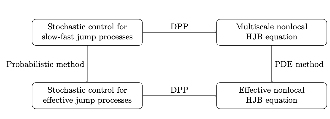
Figure 1: Relationship in this paper

The paper is organized as follows. In Section 2, we present the main results of this paper and provide some regularity and dissipative assumptions for the drift term $b$ and $c$, as well as assumptions for the utility function $g$ and the running cost $L$. In Section 3, we will study the weak averaging principle for the multiscale system (1.1) using the tightness argument. In Section 4, we will prove the convergence results for the viscosity solution to the associated nonlocal HJB equations using the perturbed test function method. Section 5 will be reserved for some concluding remarks.

To end the introduction, we list the notations that will be used frequently in the sequel. The letter $C$ denotes a positive constant whose value may change from one line to another. The notation $C_{p}$ is used to emphasize that the constant depends only on a parameter $p$, while $C(\cdots)$ is used for the case that there is more than one parameter. We use $\otimes$, $\langle\cdot,\cdot\rangle$, and $|\cdot|$ to denote the tensor product, inner product and norm in Euclidean space, respectively. We also use $\nabla$ to denote the gradient operator in Euclidean space. For any positive integer $k,l$ and probability measure $\mu$, we introduce the following function spaces:

$$\mathcal{B}_{b}(\mathbb{R}^{n}):=\left\{h:\mathbb{R}^{n}\rightarrow\mathbb{R}\mid h\text{ is bounded Borel measurable}\right\},$$

$$\mathcal{C}_{0}(\mathbb{R}^{n}):=\left\{h:\mathbb{R}^{n}\rightarrow\mathbb{R}\mid h\text{ is continuous and has compact support}\right\},$$

$${\mathcal{C}}^{k}(\mathbb{R}^{n}):=\left\{h:\mathbb{R}^{n}\rightarrow\mathbb{R}\mid h\text{ and all its partial derivatives up to order $k$ are continuous}\right\},$$

$${\mathcal{C}}^{k}_{b}(\mathbb{R}^{n}):=\left\{h\in{\mathcal{C}}^{k}(\mathbb{R}^{n})\mid\text{ for $1\leq i\leq k$, the $i$-th order partial derivatives of $h$ are bounded}\right\},$$

$${\mathcal{C}}^{k,l}_{b}(\mathbb{R}^{n}\times\mathbb{R}^{m}):=\left\{h(x,y)\mid\text{ for $1\leq|\beta|_{1}\leq k$ and $1\leq|\beta|_{2}\leq l$, $\nabla^{\beta_{1}}_{x}\nabla^{\beta_{2}}_{y}h$ is uniformly bounded}\right\},$$

$${\mathcal{C}}^{\cdot,k,l}_{b}(\mathbb{R}\times\mathbb{R}^{n}\times\mathbb{R}^{m}):=\left\{h(t,x,y)\mid\text{ for $1\leq|\beta|_{1}\leq k$ and $1\leq|\beta|_{2}\leq l$, $\nabla^{\beta_{1}}_{x}\nabla^{\beta_{2}}_{y}h$ is uniformly bounded}\right\}.$$

We equip the space $\mathcal{C}_{0}(\mathbb{R}^{n})$ with the norm $\|h\|_{0}=\sup_{x\in\mathbb{R}^{n}}|h(x)|$ and ${\mathcal{C}}^{k}(\mathbb{R}^{n})$ with the norm $\|h\|_{k}=\|h\|_{0}+\sum_{j=1}^{k}\|\nabla^{\otimes j}h\|$. Then $({\mathcal{C}}^{k}(\mathbb{R}^{n}),\|\cdot\|_{k})$ is a Banach space.

2 Assumptions and the main results

To guarantee the well-posedness of the slow-fast SDE (1.1) and the ergodicity of the fast dynamics $Y^{\epsilon}_{t}$, we need some regularity and dissipative assumptions for drifts $b$, $c$.

($\bf{A_{c}}$): Suppose that $c$ is Lipschitz continuous in $(x,y)$ uniformly, and linear growth in $y$. That is, there exist positive constants $C_{1},C_{2}$ such that for all $x_{1},x_{2}\in\mathbb{R}^{n}$, $y_{1},y_{2}\in\mathbb{R}^{m}$,

$$|c(x_{1},y_{1},v)-c(x_{2},y_{2},v)|\leq C_{1}(|x_{1}-x_{2}|+|y_{1}-y_{2}|),$$

and

$$\left|c(x_{1},y_{1})\right|\leq C_{2}(1+|y_{1}|).$$

Moreover, there exist a positive constant $\beta>0$ so that for every $x\in\mathbb{R}^{n}$ and $y,y_{1},y_{2}\in\mathbb{R}^{m}$,

$$\langle c(x,y_{1})-c(x,y_{2}),y_{1}-y_{2}\rangle\leq-\beta|y_{1}-y_{2}|^{2}.$$ (2.1)

($\bf{A_{b}}$): Assume that the function $b$ is Lipschitz continuous in $(x,y)$ uniformly with respect to $v\in\mathcal{U}$ and linear growth in $x$, i.e., there exist positive constants $K_{1},K_{2}$ such that for all $x,x_{1},x_{2}\in\mathbb{R}^{n}$, $y,y_{1},y_{2}\in\mathbb{R}^{m}$, and $v\in\mathcal{U}$,

$$|b(x_{1},y_{1},v)-b(x_{2},y_{2},v)|\leq K_{1}(|x_{1}-x_{2}|+|y_{1}-y_{2}|),$$

and

$$\left|b(x,y,v)\right|\leq K_{2}(1+|x|).$$

Remark 1.

Under assumption ($\bf{A_{c}}$) and ($\bf{A_{b}}$), the SDE (1.1) has a unique strong solution $({X^{\epsilon}},{Y^{\epsilon}})$, see e.g. [2].

For the study of stochastic control problems subject to controlled slow-fast jump diffusions (1.1), we also require the following assumptions for the utility function $g$ and running cost $L$.
($\bf{A_{L}}$): The running cost $L$ is uniformly Lipschitz continuous in $x$, with uniform continuity in $v$. Moreover, there exists a constant $K>0$ so that

$$\quad\sup_{y\in\mathbb{R}^{m},v\in\mathcal{U}}|L(x,y,v)|\leq K(1+|x|),\quad\sup_{x\in\mathbb{R}^{n},v\in\mathcal{U}}|\nabla_{y}L(x,y,v)|\leq K.$$ (2.2)

($\bf{A_{g}}$): The utility function $g$ is Lipschitz continuous in $x$ and $y$, with uniform continuity in $v$. Moreover, there exists a constant $K>0$ so that

$$\sup_{y\in\mathbb{R}^{m}}|g(x,y)|\leq K(1+|x|).$$ (2.3)

In the probabilistic method, we need to add the following stronger regularity assumption for drifts $b$, $c$, and the utility function $g$:
($\bf{A_{r}}$): Assume that $c\in\mathcal{C}^{3,3}_{b}(\mathbb{R}^{n}\times\mathbb{R}^{m})$, $g\in\mathcal{C}^{3,3}_{b}(\mathbb{R}^{n}\times\mathbb{R}^{m})$, and for every fixed $v\in\mathcal{U}$, $b(\cdot,\cdot,v)\in C^{2,3}_{b}(\mathbb{R}^{n}\times\mathbb{R}^{m})$.

Remark 2.

Under assumptions $(\bf{A_{b}})$ and $(\bf{A_{L}})$, the Hamiltonian

$$H(x,y,p_{x}):=\sup_{v\in\mathcal{U}}\left[b(x,y,v)\cdot p_{x}-L(x,y,v)\right].$$ (2.4)

is Lipschitz continuous in $x,y$, and $p_{x}$.

Now we introduce the following frozen equation:

$$dY^{x^{\prime},y}_{s}=c(x^{\prime},Y^{x^{\prime},y}_{s})ds+d\textbf{L}^{\alpha_{2}}_{s},\quad Y^{x^{\prime},y}_{t}=y\in\mathbb{R}^{m}.$$ (2.5)

The dissipative assumption ($\bf{A_{c}}$) implies that the jump process $Y^{x^{\prime}}_{s}$ has an unique ergodic measure $\mu^{x^{\prime}}$, see e.g. [34, Lemma 2].

By taking the average over the ergodic measure $\mu^{x}$ of fast component $Y^{\epsilon}$, we introduce the following effective stochastic control problem

$$u(t,x)=\sup_{v\in\mathcal{U}}\bar{J}(t,x,v):=\mathbb{E}\left(-\int^{T}_{t}e^{\lambda(s-T)}\bar{L}(\bar{X}_{s},v(s))ds+e^{\lambda(t-T)}\bar{g}(\bar{X}_{T})|\bar{X}_{t}=x\right).$$ (2.6)

where

$$\bar{L}(x,v)=\int_{\mathbb{R}^{m}}L(x,y,v)\mu^{x}(dy).$$ (2.7)

and

$$\bar{g}(x)=\int_{\mathbb{R}^{m}}g(x,y)\mu^{x}(dy).$$ (2.8)

By the dynamic programming principle, the value function $u$ in the effective stochastic control problem (2.6) is determined by the viscosity solution of the effective HJB equation:

$$\left\{\begin{aligned} &\partial_{t}u(t,x)=\Delta_{x}^{\alpha/2}u(t,x)+\bar{H}(x,\nabla_{x}u(t,x))+\lambda u(t,x).\\ &u(T,x)=\bar{g}(x),\end{aligned}\right.$$ (2.9)

where the effective Hamiltonian is given

$$\bar{H}(y,p)=\int_{\mathbb{R}^{m}}H(x,y,p)d\mu^{x}(y).$$ (2.10)

The averaging principle for two-time scale stochastic control systems with $\alpha$-stable noise is stated next.

Theorem 2.1.

Under assumptions $(\bf{A_{b}})$, $(\bf{A_{c}})$, $(\bf{A_{g}})$, $(\bf{A_{L}})$, the value function $u^{\epsilon}$ to the multiscale stochastic control problem (1.2) locally converges uniformly on compact subsets of $\mathbb{R}^{+}\times\mathbb{R}^{n}$ to the value function $\bar{u}$ to the effective stochastic control problem (2.6), i.e., for every $l,T>0$, $y\in\mathbb{R}^{m}$ we have

$$\lim_{\epsilon\to 0}\sup_{t\in[0,T]}\sup_{|x|<l}|u^{\epsilon}(t,x,y)-u(t,x)|=0.$$

Remark 3.

By dynamic programming principle, the above averaging principle for value function $u^{\epsilon}$ is equivalent to the singular perturbation problems for the nonlocal HJB equation (1.4). Consequently, our results in this paper extend the previous research on singular perturbation problems for the second-order HJB equation, as studied by Alvarez and Bardi [1].

3 Probabilstic method

In this section, we will prove the averaging principle in Theorem 2.1 using the probabilistic method. Specifically, we will show that the value function of the original multiscale stochastic control system converges to the value function of the effective stochastic control system. This will be achieved by proving the weak averaging principle of the controlled jump diffusions.

3.1 Weak averaging principle of the controlled jump diffusion

To establish the tightness, we provide the following exponential ergodicity for equation (2.5), inspired by [34, Proposition 1]. The detailed proof is omitted.

Proposition 3.1.

Under Hypothesis ($\bf{A_{c}}$), for each function $\widetilde{\varphi}(y)\in C^{1}_{b}$, there exist positive constants $C$ and $\gamma$ such that for all $s\geq 0$ and $x^{\prime}\in\mathbb{R}^{n}$, we have

$$\sup_{x^{\prime}\in\mathbb{R}^{n}}|P^{x^{\prime}}_{s}\widetilde{\varphi}(y)-\mu^{x^{\prime}}(\widetilde{\varphi})|\leq C\|\widetilde{\varphi}\|_{0}e^{-\frac{\gamma s}{8}}(1+|y|^{\frac{1}{2}}),$$

where $P^{x^{\prime}}_{s}\widetilde{\varphi}(y)=\mathbb{E}\widetilde{\varphi}(Y^{x^{\prime},y}_{s})$.

In the following, we show that as the scale parameter $\epsilon\to 0$, the slow component $X^{\epsilon}$ of the original system weakly converges to the averaged system $\bar{X}$ in law sense. Note that the sample paths of $X^{\epsilon}$ are almost surely contained in the càdlàg space $\mathbb{D}([t,T];\mathbb{R}^{n})$, which consists of real-valued right-continuous functions with left limits. It is well-known that the càdlàg space $\mathbb{D}([t,T];\mathbb{R}^{m})$ equipped with the Skorokhod metric

$$d_{\mathbb{R}}(\omega_{1},\omega_{2})=\inf\left\{\epsilon>0:\sup_{r\in\mathbb{R}}\left|\omega_{1}(r)-\omega_{2}(\lambda(r))\right|\leq\epsilon,\sup_{s\neq r}\left|\ln\frac{\arctan(\lambda(r))-\arctan(\lambda(s))}{\arctan(r)-\arctan(s)}\right|\leq\epsilon\right\}$$

is a Polish space (e.g., [22, Section VI.1] or [11, Section 14]).

The following lemma shows the tightness of $\{X^{\epsilon},\epsilon>0\}$ on the càdlàg space $\mathbb{D}\left([t,T],\mathbb{R}^{n}\right)$, which proof is a minor adaptation of the proofs from the sections in [34, Lemma 7], and it is left in Appendix A.

Lemma 3.2.

If hypotheses ($\bf{A_{b}}$), ($\bf{A_{c}}$) hold, then the family $\{X^{\epsilon},\epsilon>0\}$ is relative compact in the càdlàg space $\mathbb{D}\left([t,T],\mathbb{R}^{n}\right)$.

Next, we will present the uniform approximation of càdlàg functions by step functions, which comes from [18, Lemma 9, Appendix A].

Lemma 3.3.

Let $h\in\mathbb{D}\left([t,T],\mathbb{R}^{n}\right)$. If $(t^{n}_{k})$ is a sequence of subdivisions $t=t^{n}_{0}<t_{1}<\cdots<t^{n}_{k_{n}}=T$ of $[t,T]$ such that

$$\sup_{0\leq i\leq k-1}|t^{n}_{i+1}-t^{n}_{i}|\rightarrow 0,~{}~{}\sup_{s\in[t,T]\backslash\{t^{n}_{0},\cdots,t^{n}_{k_{n}}\}}|\Delta h(s)|\rightarrow 0,~{}~{}as~{}~{}n\rightarrow\infty.$$

Then we have the step function approximation

$$\sup_{s\in[t,T]}\left|h(s)-\sum_{0}^{k_{n}-1}h(t_{i})I_{t^{n}_{i},t^{n}_{i+1}}(s)+h(t^{n}_{k_{n}})I_{t^{n}_{k_{n}}}(s)\right|\rightarrow 0.$$

Due to the tightness of the family $\{X^{\epsilon},\epsilon>0\}$, there exists a subsequence $\epsilon_{n}\rightarrow 0$ and a stochastic process $X$, such that $X^{\epsilon_{n}}$ converges weakly to $X$, as $n\rightarrow\infty$. Based on Lemma 3.3, we derive the following result using the same technique as shown in [34, Lemma 9].

Lemma 3.4.

For sufficient small $\delta>0$, there exists a positive constant $N\in\mathbb{N}$ and $\mathbb{R}^{n}$-valued left-continuous simple processes $x^{1},x^{2},\cdots,x^{N}$ such that

$$\mathbb{P}\left(\bigcap_{k=1}^{N}\left\{d_{\mathbb{R}}(X^{\epsilon_{n}},x^{k})>\delta\right\}\right)<\delta,~{}~{}\forall n\in\mathbb{N},$$

$$\mathbb{P}\left(\bigcap_{k=1}^{N}\left\{d_{\mathbb{R}}(X,x^{k})>\delta\right\}\right)<\delta.$$

In what follows, we will fix a $\delta>0$ and let $x^{1},x^{2},\cdots,x^{N}$ be the corresponding $N$ step functions in Lemma 3.4. For each $x\in\mathbb{D}([t,T];\mathbb{R}^{n})$ and $k=1,2,\cdots,N$, we define

$$\beta_{k}(x):=d_{\mathbb{R}}(x,x^{k}).$$

Let $\psi,\varphi_{1},\cdots,\varphi_{N}:\mathbb{D}\left(\left[t,T\right];\mathbb{R}^{n}\right)\rightarrow[0,1]$ be smooth mappings such that

1. $\psi(x)+\sum_{k=1}^{n}\varphi_{k}(x)=1$, $\forall x\in\mathbb{D}\left([t,T];\mathbb{R}^{n}\right)$;

2. $\mathrm{supp}\,\psi\subset\bigcap_{k=1}^{N}\left\{y;\beta_{k}(x)>\delta\right\}$;

3. $\mathrm{supp}\,\varphi_{k}\subset\bigcap_{k=1}^{N}\{y;\beta_{k}(x)<2\delta\}$, $1\leq k\leq N$.

Now we introduce the following $[0,1]$-valued random variables:

$$\xi_{n} :=\psi(X^{\epsilon_{n}}),~{}~{}~{}~{}\xi:=\psi(X),$$ (3.1)

$$\eta^{k}_{n} :=\varphi_{k}(X^{\epsilon_{n}}),~{}~{}~{}~{}\eta^{k}:=\varphi_{k}(X),$$

and two measurable sets

$$\widetilde{A}_{n} :=\bigcap^{N}_{k=1}\left\{\omega;d_{\mathbb{R}}(X^{\epsilon_{n}}(\omega),x^{k}(\omega))>\delta\right\},~{}~{}\widetilde{A} :=\bigcap^{N}_{k=1}\left\{\omega;d_{\mathbb{R}}(X(\omega),x^{k}(\omega))>\delta\right\}.$$

Then Lemma 3.4 implies that

$$\mathrm{supp}\,\xi_{n}:=\left\{\omega\in\Omega;\xi_{n}(\omega)\neq 0\right\}\subseteq\widetilde{A}_{n},~{}~{}~{}\mathrm{supp}\,\xi:=\left\{\omega\in\Omega;\xi(\omega)\neq 0\right\}\subseteq\widetilde{A}.$$

Set

$$\Gamma_{n}(s) :=\left[\phi(X^{\epsilon_{n}}_{s})-\phi(X^{\epsilon_{n}}_{t_{0}})-\int^{s}_{t_{0}}\left\langle\nabla_{x}\phi(X^{\epsilon_{n}}_{r}),b(X^{\epsilon_{n}}_{r},Y^{\epsilon_{n}}_{r},v_{r})\right\rangle dr-\int^{s}_{t_{0}}\left(-\left(-\Delta_{x}\right)^{\frac{\alpha_{1}}{2}}\phi(X^{\epsilon_{n}}_{r})\right)dr\right]\Phi_{t_{0}}(X^{\epsilon_{n}}),$$ (3.2)

where $\phi$ is a $C^{\infty}_{0}$ function on $\mathbb{R}^{n}$. The function $\Phi_{{t_{0}}}(\cdot)$ is a bounded function on $\mathbb{D}\left(\left[t,T\right]\right)$, and measurable with respect to the sigma-field $\sigma\left(\omega_{s},\omega\in\mathbb{D}\left(\left[t,T\right]\right),t\leq s\leq t_{0}\right)$.

Using Itô’s formula [2, Theorem 4.4.7], we have

$$\phi(X^{\epsilon_{n}}_{s})-\phi(x)= \ \int^{s}_{t}\left\langle\nabla_{x}\phi(X^{\epsilon_{n}}_{r}),b(X^{\epsilon_{n}}_{r},Y^{\epsilon_{n}}_{r},v_{r})\right\rangle dr+\int^{s}_{t}\left(-\left(-\Delta_{x}\right)^{\frac{\alpha_{1}}{2}}\phi(X^{\epsilon_{n}}_{r})\right)dr$$ (3.3)

$$+\int^{s}_{t}\int_{\mathbb{R}^{n}\backslash\{0\}}\left[\phi(X^{\epsilon_{n}}_{r-}+x)-\phi(X^{\epsilon_{n}}_{r-})\right]\widetilde{N}_{1}(dr,dx).$$

Since the integral $\int^{s}_{t}\int_{\mathbb{R}^{n}\backslash\{0\}}\cdot~{}~{}\widetilde{N}_{1}(dr,dx)$ in $\mathbb{R}^{n}$ is a martingale with respect to the $\sigma$-algebra $\mathcal{F}_{s}$ generated by $\left\{\widetilde{N}_{1}(r,dx);r\leq s\right\}$, we have

$$\mathbb{E}\left[\int^{s}_{t_{0}}\int_{\mathbb{R}^{n}\backslash\{0\}}\left[\phi(X^{\epsilon}_{r-}+x)-\phi(X^{\epsilon}_{r-})\right]\widetilde{N}_{1}(dr,dx)\Phi_{t_{0}}(X^{\epsilon})\right|X^{\epsilon}_{t}=x,Y^{\epsilon}_{t}=y]=0.$$ (3.4)

In view of (3.2)-(3.4), we get

$$\mathbb{E}\left[\Gamma_{n}(s)|X^{\epsilon}_{t}=x,Y^{\epsilon}_{t}=y\right]\to 0,~{}~{}n\to\infty.$$ (3.5)

We have the following result using the same approach of [34, Lemma 10].

Lemma 3.5.

For every $\delta>0$ and each positive integral $k=1,2,\cdots,N$, there exists a positive integer $M_{0}$, such that $|X^{\epsilon_{n}}_{s}-x^{k}_{s}|\leq\delta$, we have

$$\sum_{k=1}^{N}\mathbb{E}\left[(\Gamma_{n}(r)-\Gamma^{k}_{n}(s))\eta^{k}_{n}(s)\right]\leq M_{0}\delta,$$

where $\Gamma^{k}_{n}(s)$ is defined by

$$\Gamma^{k}_{n}(s)=\left[\phi(x^{k}_{s})-\phi(x^{k}_{t_{0}})-\int^{s}_{t_{0}}\left\langle\nabla_{x}\phi(x^{k}_{r}),b(x^{k}_{r},Y^{\epsilon_{n}}_{r},v_{r})\right\rangle dr-\int^{s}_{t_{0}}\left(-\left(-\Delta_{x}\right)^{\frac{\alpha_{1}}{2}}\phi(x^{k}_{r})\right)dr\right]\Phi_{t_{0}}(x^{k}).$$ (3.6)

Now, we can infer the moment estimate for the slow component $X_{t}^{\epsilon}$.

Proposition 3.6.

Under Hypothesis ($\bf{A_{b}}$), for each $1\leq p<\alpha_{1}$, we have

$$\sup_{0<\epsilon\leq 1}\mathbb{E}\left(\sup_{t\leq s\leq T}|X^{\epsilon}_{s}|^{p}\right)\leq C_{p,K_{2},T}(1+|x|^{p}).$$ (3.7)

Proof.

By applying the Hölder inequality, we have

$$|X^{\epsilon}_{s}|^{p} =C_{p}|x|^{p}+C_{p,T}\int^{s}_{t}|b({X^{\epsilon}_{r}},{Y^{\epsilon}_{r}},v_{r}|^{p}dr+|\textbf{L}_{s}^{{\alpha}_{1}}|^{p},\;\;X^{\epsilon}_{t}=x\in\mathbb{R}^{n}.$$ (3.8)

For any $s\in[0,T]$, by assumptions ($\bf{A_{b}}$), we obtain

$$\mathbb{E}\left[\sup_{t\leq s\leq T}|X^{\epsilon}_{t}|^{p}\right]\leq C_{p,K_{2}}\left(1+|x|^{p}\right)+C_{p,T}\int^{T}_{t}\mathbb{E}|X^{\epsilon}_{r}|^{p}dr.$$ (3.9)

Furthermore, by using Grönwall inequality, we yield

$$\sup_{0<\epsilon\leq 1}\mathbb{E}\left[\sup_{t\leq s\leq T}|X^{\epsilon}_{s}|^{p}\right]\leq C_{p,K_{2},T}(1+|x|^{p}).$$

∎

The following result will play an important role below.

Lemma 3.7.

Let $f\in\mathcal{C}^{0,1,1,0}_{b}$ and $\bar{f}(s,x^{\prime},v_{s}):=\int_{\mathbb{R}^{n}}f(s,x^{\prime},y,v_{s})\mu^{x^{\prime}}(dy)$, then for every $t<s<T$, we have

$$\mathbb{E}\left|\int^{T}_{s}\left(f(r,x^{k}_{r},Y^{\epsilon_{n}}_{r},v_{r})-\bar{f}(r,x^{k}_{r},v_{r})\right)dr\right|\rightarrow 0,~{}~{}as~{}~{}n\rightarrow\infty.$$

Proof.

Set $\widetilde{X}^{\epsilon}_{s^{\prime}}=X^{\epsilon}_{s-t}$ and $\widetilde{Y}^{\epsilon}_{s^{\prime}}=Y^{\epsilon}_{s-t}$. By the equation (1.1), we have

$$\left\{\begin{aligned} d{\widetilde{X}^{\epsilon}_{s^{\prime}}}&=b({\widetilde{X}^{\epsilon}_{s^{\prime}}},{\widetilde{Y}^{\epsilon}_{s^{\prime}}},v_{{s^{\prime}}})d{s^{\prime}}+d\textbf{L}_{s^{\prime}}^{{\alpha}_{1}},\quad\widetilde{X}^{\epsilon}_{0}=x,\\ d{\widetilde{Y}^{\epsilon}_{s^{\prime}}}&=\frac{1}{\epsilon}c({\widetilde{X}^{\epsilon}_{s^{\prime}}},\widetilde{Y}^{\epsilon}_{s^{\prime}})d{s^{\prime}}+\epsilon^{-\frac{1}{\alpha_{2}}}d\textbf{L}_{s^{\prime}}^{{\alpha_{2}}},\quad\widetilde{Y}^{\epsilon}_{0}=y.\\ \end{aligned}\right.$$ (3.10)

Let $(a_{k},b_{k})\subseteq[0,T-t]$ be an interval on which $x^{k}_{\cdot}$ is a constant, denoted by $z^{k}$. This can be done by Lemma 3.3. Then we will only show

$$\mathbb{E}\left|\int^{b_{k}}_{a_{k}}\left[f(r,z^{k},\widetilde{Y}^{\epsilon_{n}}_{r},v_{r})-\bar{f}(r,z^{k},v_{r})\right]dr\right|\rightarrow 0,~{}~{}as~{}~{}n\rightarrow\infty.$$

Rescaling the equation (3.10), we have

$$\left\{\begin{aligned} \widetilde{X}^{\epsilon_{n}}_{{s^{\prime}}\epsilon_{n}}&=x+\epsilon_{n}\int^{{s^{\prime}}}_{0}b\left(\widetilde{X}^{\epsilon_{n}}_{r^{\prime}\epsilon_{n}},\widetilde{Y}^{\epsilon_{n}}_{r^{\prime}\epsilon_{n}},v_{r^{\prime}\epsilon_{n}}\right)dr^{\prime}+\textbf{L}^{\alpha_{1}}_{{s^{\prime}}\epsilon_{n}},\\ \widetilde{Y}^{\epsilon_{n}}_{{s^{\prime}}\epsilon_{n}}&=y+\int^{{s^{\prime}}}_{0}c\left(\widetilde{X}^{\epsilon_{n}}_{r^{\prime}\epsilon_{n}},\widetilde{Y}^{\epsilon_{n}}_{r^{\prime}\epsilon_{n}}\right)dr^{\prime}+\widetilde{\textbf{L}}^{\epsilon,\alpha_{2}}_{s^{\prime}},\end{aligned}\right.$$

where $\widetilde{\textbf{L}}^{\epsilon,\alpha_{2}}_{r}$ is defined by

$$\widetilde{\textbf{L}}^{\epsilon,\alpha_{2}}_{r}=\epsilon^{-\frac{1}{\alpha_{2}}}\textbf{L}^{\alpha_{2}}_{\epsilon r}.$$

Obviously, the process $\widetilde{\textbf{L}}^{\alpha_{2}}_{s}$ is an $\alpha$-stable process, with the same law as $\textbf{L}^{\alpha_{2}}_{s}$. Then by Hypotheses ($\bf{A_{b}}$), Proposition 2, and the inequality (2.8) in [16], we have

$$\mathbb{E}\left|\widetilde{{X}}^{\epsilon_{n}}_{s\epsilon_{n}}-x\right| \leq\epsilon_{n}\mathbb{E}\int^{s}_{0}|b\left(\widetilde{{X}}^{\epsilon_{n}}_{r^{\prime}\epsilon_{n}},\widetilde{{Y}}^{\epsilon_{n}}_{r^{\prime}\epsilon_{n}},v_{r^{\prime}\epsilon_{n}}\right)|dr^{\prime}+\mathbb{E}|\textbf{L}^{\alpha_{1}}_{s\epsilon_{n}}|\to 0,~{}~{}n\to\infty.$$ (3.11)

On the one hand, we know

$$\mathbb{E}\left|\widetilde{{Y}}^{\epsilon_{n}}_{r\epsilon_{n}}-{{Y}}^{x,y}_{r}\right| =\mathbb{E}\left|\int^{r}_{0}c(\widetilde{X}^{\epsilon_{n}}_{r^{\prime}\epsilon_{n}},\widetilde{Y}^{\epsilon_{n}}_{r^{\prime}\epsilon_{n}})dr^{\prime}-\int^{r}_{0}c(x,{Y}^{{x},{y}}_{r^{\prime}})dr^{\prime}\right|$$

$$\leq\|\nabla_{y}c\|_{0}\int^{r}_{0}\mathbb{E}|\widetilde{Y}^{\epsilon_{n}}_{r^{\prime}\epsilon_{n}}-{Y}^{x,y}_{r^{\prime}}|dr^{\prime}+\|\nabla_{x}c\|_{0}\int^{r}_{0}\mathbb{E}|\widetilde{X}^{\epsilon_{n}}_{r^{\prime}\epsilon_{n}}|dr^{\prime}.$$

By applying Grönwall’s inequality and (3.11), we have

$$\mathbb{E}\left|\widetilde{Y}^{\epsilon_{n}}_{r\epsilon_{n}}-{Y}^{x,y}_{r}\right|\to 0,~{}~{}n\to\infty.$$ (3.12)

By the result of Proposition 3.1 and using the same technique as shown in (3.12), for $f\in\mathcal{C}^{0,1,1,0}_{b}$, we obtain

$$\ \mathbb{E}\left|\int^{b_{k}}_{a_{k}}\left[f(r,z^{k},\widetilde{Y}^{\epsilon_{n}}_{r},v_{r})-\bar{f}(r,z^{k},v_{r})\right]ds\right|$$

$$= \epsilon_{n}\mathbb{E}\left|\int^{b_{k}/{\epsilon_{n}}}_{a_{k}/{\epsilon_{n}}}\left[f(r\epsilon_{n},z^{k},\widetilde{Y}^{\epsilon_{n}}_{r{\epsilon_{n}}},v_{r\epsilon_{n}})-\bar{f}(r\epsilon_{n},z^{k},v_{r\epsilon_{n}})\right]dr\right|$$

$$\leq \ \epsilon_{n}\mathbb{E}\left|\int^{b_{k}/{\epsilon_{n}}}_{a_{k}/{\epsilon_{n}}}\left[f(r\epsilon_{n},z^{k},\widetilde{Y}^{\epsilon_{n}}_{r{\epsilon_{n}}},v_{r\epsilon_{n}})-f(r\epsilon_{n},z^{k},{Y}^{z^{k},y}_{r},v_{r\epsilon_{n}})\right]dr\right|$$

$$\ +\epsilon_{n}\left|\int^{b_{k}/{\epsilon_{n}}}_{a_{k}/{\epsilon_{n}}}\mathbb{E}\left(f(r\epsilon_{n},z^{k},{Y}^{z^{k},y}_{r},v_{r\epsilon_{n}})\right)dr-\int^{b_{k}/{\epsilon_{n}}}_{a_{k}/{\epsilon_{n}}}\int_{\mathbb{R}^{n}}f(r\epsilon_{n},z^{k},y,v_{r})\mu^{z^{k}}(dy)dr\right|$$

$$\leq \ \epsilon_{n}\|\nabla_{y}f\|_{0}\int^{b_{k}/{\epsilon_{n}}}_{a_{k}/{\epsilon_{n}}}\mathbb{E}|\widetilde{Y}^{\epsilon_{n}}_{r{\epsilon_{n}}}-{Y}^{z^{k},y}_{r}|dr+\epsilon_{n}\int^{b_{k}/{\epsilon_{n}}}_{a_{k}/{\epsilon_{n}}}C\|f\|_{0,0,1,0}e^{-\gamma r}\left(1+|y|^{\frac{1}{2}}\right)dr$$

$$\to \ 0,~{}~{}n\to\infty.$$

This proof is finished. ∎

Now, we state that the slow component $X^{\varepsilon}$ converges weakly to $X$ in the law sense.

Proposition 3.8.

Under Hypotheses ($\bf{A_{b}}$) and ($\bf{A_{c}}$) given in Section 2, the slow component $X^{\epsilon}$ converges weakly to a limit process $X$ as $\epsilon$ goes to zero. Moreover, the limit process $X$ is the unique solution to the martingale problem associated with the following generator

$$\mathcal{L}_{1}=-\left(-\Delta_{x}\right)^{\frac{\alpha_{1}}{2}}+{\bar{b}}(x,v)\cdot\nabla_{x},$$

where $\bar{b}$ is the homogenized drift given by $\bar{b}(x,v)=\int_{\mathbb{R}^{n}}b(x,y,v){\mu^{x}}(dy)$, and $\mu^{x}$ is an invariant measure of the corresponding frozen equation (2.5). That is, for every $t\leq t_{0}<s\leq T$, $\phi\in C^{\infty}_{0}(\mathbb{R}^{m})$ and any bounded function $\Phi$ on $\mathbb{D}\left([t,T];\mathbb{R}^{m}\right)$ which is measurable with respect to the $\sigma$-field $\sigma\left(\omega_{s}:\omega\in\mathbb{D}\left([t,T];\mathbb{R}^{m}\right),t_{0}\leq s\leq t\right)$,

$$\mathbb{E}\left[\left(\phi(X_{s})-\phi(X_{t_{0}})-\int^{s}_{t_{0}}\mathcal{L}_{1}\phi(X_{r})dr\right)\Phi(X)\right]=0.$$

Proof.

We follow the approach of [34, Theorem 1]. By Lemma 3.2, there exists a subsequence $\{\epsilon_{n}\}\rightarrow 0$, such that $X^{\epsilon_{n}}$ converges weakly to a limit point $X$, as $n\rightarrow\infty$.

Set

$$\Gamma(s)=\left[\phi(X_{s})-\phi(X_{t_{0}})-\int^{s}_{t_{0}}\left\langle\nabla_{x}\phi(X_{r}),{\bar{b}}(X_{r},v_{r})\right\rangle dr-\int^{s}_{t_{0}}\left(-\left(-\Delta_{x}\right)^{\frac{\alpha_{1}}{2}}\phi(X_{r})\right)dr\right]\Phi_{t_{0}}(X),$$

where the function ${\bar{b}}(x^{\prime},v_{s})$ is defined by

$$\bar{b}(x^{\prime},v)=\int_{\mathbb{R}^{m}}b(x^{\prime},y,v)\mu^{x^{\prime}}(dy).$$

For any $p,q>1$ and $\frac{1}{p}+\frac{1}{q}=1$, by Hölder inequality, Lemma 3.4 and $\phi\in C^{\infty}_{0}$, we have

$$|\mathbb{E}\left(\Gamma_{n}(s)\xi_{n}(s)\right)| \leq\left(\mathbb{E}(\Gamma_{n}(s))^{p}\right)^{1/p}\left(\mathbb{P}(\widetilde{A}_{n}(s))\right)^{1/q}\leq C\delta^{1/q},$$ (3.13)

$$|\mathbb{E}\left(\Gamma(s)\xi(s)\right)| \leq\left(\mathbb{E}(\Gamma(s))^{p}\right)^{1/p}\left(\mathbb{P}(\widetilde{A}(s))\right)^{1/q}\leq C\delta^{1/q}.$$

Since $\eta^{k}_{n}\Rightarrow\eta^{k}$ and $\eta^{k}_{n}\leq 1$. Thus for each $k=1,2,\cdots,N$, we have

$$\left|\mathbb{E}\left(\Gamma^{n}_{k}\eta^{k}_{n}-\Gamma^{k}\eta^{k}\right)\right| \leq\mathbb{E}\left|\left(\Gamma^{n}_{k}-\Gamma^{k}\right)\eta^{k}_{n}\right|+|\eta^{k}|\left|\mathbb{E}\left(\eta^{k}_{n}-\eta^{k}\right)\right|\leq\mathbb{E}\left|\Gamma^{n}_{k}-\Gamma^{k}\right|+\mathbb{E}\left|\eta^{k}_{n}-\eta^{k}\right|\times\Gamma^{k}.$$ (3.14)

By the definitions of $\psi$ and $\varphi$, we yield

$$\mathbb{E}\left(\Gamma_{n}\xi_{n}(s)\right)+\sum_{k=1}^{N}\mathbb{E}_{x,y}\left(\Gamma_{n}\eta^{k}_{n}(s)\right)\rightarrow 0,~{}~{}as~{}~{}n\rightarrow\infty,~{}~{}\mathbb{E}(\Gamma)=\mathbb{E}(\Gamma\xi_{s})+\sum_{k=1}^{N}\mathbb{E}_{x,y}\left(\Gamma\eta^{k}_{s}\right),$$

and

$$\sum_{k=1}^{N}\mathbb{E}(\Gamma_{n}\eta^{k}_{n}) =\sum_{k=1}^{N}\mathbb{E}\left[(\Gamma_{n}-\Gamma^{k}_{n})\eta^{n}_{k}\right]+\sum_{k=1}^{N}\mathbb{E}(\Gamma^{k}_{n}\eta^{k}_{n}),$$ (3.15)

$$\sum_{k=1}^{N}\mathbb{E}(\Gamma\eta^{k}) =\sum_{k=1}^{N}\mathbb{E}\left[(\Gamma-\Gamma^{k})\eta_{k}\right]+\sum_{k=1}^{N}\mathbb{E}(\Gamma^{k}\eta^{k}).$$

By Lemma 3.5, (3.13), (3.14) and (3.15), we get

$$\mathbb{E}[\Gamma_{n}]\rightarrow\mathbb{E}[\Gamma],~{}~{}\text{as}~{}~{}n\rightarrow\infty.$$ (3.16)

Combining (3.5) and (3.16), we have

$$\mathbb{E}\left[\left(\phi(X_{s})-\phi(X_{t_{0}})-\int^{s}_{t_{0}}\mathcal{L}_{1}\phi(X_{r})dr\right)\Phi_{t_{0}}(X_{r})\right]=0,$$

where

$$\mathcal{L}_{1}\phi(x)=\left\langle\nabla_{x}\phi(x),{\bar{b}}(x,v)\right\rangle-\left(-\Delta_{x}\right)^{\frac{\alpha_{1}}{2}}\phi(x).$$

∎

Then according to Proposition 3.8, the averaged controlled jump diffusion $\bar{X}_{s}$ is given by

$$d\bar{X}_{s}=\bar{b}(X_{s},v_{s})ds+d\textbf{L}^{\alpha_{1}}_{s},\quad\bar{X}_{t}=x\in\mathbb{R}^{n},$$ (3.17)

where $\bar{b}(x^{\prime},v)=\int_{\mathbb{R}^{m}}b(x^{\prime},y,v)d\mu^{x^{\prime}}(y)$.

3.2 Proof of Theorem 2.1

Now, we are in the position to give proof of Theorem 2.1. We divide the proof into the following two steps.
Step 1. We first prove that for every $x,y$, the cost function $J^{\epsilon}(x,y,v)$ converges to the effective cost function $\bar{J}(x,v)$, i.e.,

$$\lim_{\epsilon\to 0}J^{\epsilon}(x,y,v)=\bar{J}(x,v).$$ (3.18)

By Lemma 3.7, for every $x\in\mathbb{R}^{n},y\in\mathbb{R}^{m}$, we have

$$\lim_{\epsilon\to 0}\mathbb{E}\left[-\int^{T}_{t}e^{\lambda(r-T)}L\left(X^{\epsilon}_{r},Y^{\epsilon}_{r},v(r)\right)dr|X^{\epsilon}_{t}=x,Y^{\epsilon}_{t}=y\right]=\mathbb{E}\left[-\int^{T}_{t}e^{\lambda(r-T)}\bar{L}\left(\bar{X}_{r},v(r)\right)dr|\bar{X}_{t}=x\right],$$ (3.19)

where $\bar{L}$ is defined by

$$\bar{L}(x,v)=\int_{\mathbb{R}^{m}}L(x,y,v)\mu^{x}(dy).$$

For the terminal cost function $g$, we have

$$\mathbb{E}\left[e^{\lambda(t-T)}g\left(X^{\epsilon}_{T},Y^{\epsilon}_{T}\right)|X^{\epsilon}_{t}=x,Y^{\epsilon}_{t}=y\right]=\int_{\mathbb{R}^{n}}e^{\lambda(t-T)}\mathbb{E}\left[g\left(x^{\prime},Y^{\epsilon}_{T}\right)|Y^{\epsilon}_{t}=y\right]\mu^{X^{\epsilon}_{T}}(dx^{\prime}).$$

By the ergodicity of fast component $Y^{\varepsilon}_{T}$, for every $x^{\prime}\in\mathbb{R}^{m}$ and $y\in\mathbb{R}^{n}$, we get

$$\lim_{\epsilon\to 0}\mathbb{E}\left[g\left(x^{\prime},Y^{\epsilon}_{T}\right)|Y^{\epsilon}_{t}=y\right]=\int_{\mathbb{R}^{m}}g(x^{\prime},y^{\prime})\mu^{x^{\prime}}(dy^{\prime})=\bar{g}(x^{\prime}).$$

Utilizing the convergence result of the slow component $X^{\epsilon}_{t}$ [32, Theorem 2.3], we have

$$\lim_{\epsilon\to 0}\mathbb{E}\left[e^{\lambda(t-T)}\bar{g}\left(X^{\epsilon}_{T},Y^{\epsilon}_{T}\right)|X^{\epsilon}_{t}=x,Y^{\epsilon}_{t}=y\right]= \lim_{\epsilon\to 0}\mathbb{E}\left[e^{\lambda(t-T)}\bar{g}\left(X^{\epsilon}_{T}\right)|X^{\epsilon}_{t}=x\right]$$

$$= \mathbb{E}\left[e^{\lambda(t-T)}\bar{g}\left(\bar{X}_{T}\right)|\bar{X}_{t}=x\right].$$ (3.20)

Combining (3.19) and (3.2), we get (3.18).

Step 2. Now we show that the value function $u^{\epsilon}$ converges to the effective value function $u$. Since controls $v_{s}$ taking value in the closed convex set $U\subset\mathbb{R}^{r}$, there exists an optimal control $\bar{v}^{\epsilon}$ (see e.g. [12]), such that

$$u^{\epsilon}(t,x,y):=\sup_{v\in\mathcal{U}}J^{\epsilon}(t,x,y,v)=J^{\epsilon}(t,x,y,\bar{v}^{\epsilon})$$

Since $\sup_{\epsilon>0}\bar{J}(t,x,y,\bar{v}^{\epsilon})\leq\sup_{v\in\mathscr{U}}\bar{J}(t,x,v)$, we have

$$\limsup_{\epsilon\to 0}u^{\epsilon}(t,x,y)=\limsup_{\epsilon\to 0}J^{\epsilon}(t,x,y,\bar{v}^{\epsilon})\leq\sup_{v\in\mathcal{U}}\bar{J}(t,x,v)=\bar{u}(t,x).$$

Similarly, we consider the optimal control $\bar{v}$ for $\bar{J}$, so that

$$\bar{u}(t,x):=\sup_{v\in\mathcal{U}}\bar{J}(t,x,v)=\bar{J}(t,x,\bar{v}).$$

Note that for every $\epsilon>0$, $u^{\epsilon}(t,x,y)=\sup_{v\in\mathcal{U}}J^{\epsilon}(t,x,y,v)\geq J^{\epsilon}(t,x,y,\bar{v})$. Then

$$\liminf_{\epsilon\to 0}u^{\epsilon}(t,x,y)\geq\liminf_{\epsilon\to 0}J^{\epsilon}(t,x,y,\bar{v})=\bar{J}(t,x,\bar{v})=\bar{u}(t,x).$$

Hence we have for every $v\in\mathcal{U}$, $l,T>0$,

$$\lim_{\epsilon\to 0}\sup_{t\in[0,T]}\sup_{|x|<l}|u^{\epsilon}(t,x,y)-u(t,x)|=0.$$

4 PDE method

In this section, we construct an effective Hamiltonian and initial data to demonstrate the convergence of the solution pair of the singularly perturbed optimal nonlocal HJB equation to the solution pair of the limiting optimal nonlocal HJB equation. Under certain appropriate assumptions, by applying Itô’s formula and taking expectations on both sides, the above value function $u^{\epsilon}$ mentioned above is the unique solution to a nonlocal HJB equation (1.4).

4.1 Viscosity solutions

In this subsection, we recall some preliminaries for viscosity solutions for nonlocal HJB equations. Consider the nonlocal HJB equation

$$\left\{\begin{aligned} &\partial_{t}u(t,x)=\Delta_{x}^{\alpha/2}u+H(x,\nabla u(t,x))+\lambda u(t,x),\quad(t,x)\in(0,T)\times\Omega,\\ &u(T,x)=g(x),\quad x\in\Omega,\end{aligned}\right.$$ (4.1)

Here, the discount factor $\lambda>0$, $\Omega$ is the whole space $\mathbb{R}^{n}$, or in a bounded connected smooth open domain $\Omega\subset\mathbb{R}^{n}$. If $\Omega$ is a bounded domain in $\mathbb{R}^{n}$, we also assume the Dirichlet boundary condition

$$u(x)=h(x),\quad\text{on }[0,T]\times\Omega^{c}.$$ (4.2)

where $h$ is a continuous function.

Now we recall two equivalent definitions of viscosity solutions for nonlocal HJB equations (4.1), see e.g. Barles and Imbert [8], Ciomaga [17], and Mou [26].

Definition 4.1.

A upper (lower) semicontinuous function $u:[0,T]\times\mathbb{R}^{n}\to\mathbb{R}$ is a viscosity subsolution (supersolution) to (4.1) if for any bounded test-function $\varphi\in C^{1,2}([0,T)\times\mathbb{R}^{n})$ such that $u-\varphi$ attains its global maximum (minimum) at $(t,x)\in(0,T)\times\Omega$, then

$$\partial_{t}\varphi(t,x)\leq(\geq)\Delta_{x}^{\alpha/2}\varphi(t,x)+H(x,\nabla_{x}\varphi(t,x))+\lambda u.$$

Moreover, $u$ is a viscosity solution of (4.1) if it is both a subsolution and a supersolution of (4.1).

Note that the above definition involves the maximum and minimum of $u-\varphi$ in the whole space, and it is not convenient to use in many situations. Now we give equivalent definitions for viscosity solutions, which only rely on the maximum and minimum in bounded domains. We first introduce the following localized operators

$$I^{\delta}[\varphi](x)=\int_{B_{\delta}(x)}\left[\varphi(x+z)-\varphi(x)-\langle\nabla\varphi(x),z\rangle\right]\frac{C_{n,\alpha}}{|z|^{n+\alpha}}dz,\quad x\in\mathbb{R}^{n},$$ (4.3)

and

$$I^{\delta,c}[\varphi](x)=\int_{B^{c}_{\delta}(x)}\left[\varphi(x+z)-\varphi(x)\right]\frac{C_{n,\alpha}}{|z|^{n+\alpha}}dz,\quad x\in\mathbb{R}^{n}.$$ (4.4)

where the test function $\varphi\in C^{2}(B_{\delta}(x))$ for some constant $\delta>0$.

Remark 4.

We remark that for general Lévy measure $\nu$, the localized operators are given by

$$I^{\delta}[\varphi](x)=\int_{B_{\delta}(x)}\left[u(x+z)-u(x)-1_{B_{1}(0)}(z)\langle\nabla u(x),z\rangle\right]\nu(dz),\quad x\in\mathbb{R}^{n},$$

and

$$I^{\delta,c}[\varphi,p](x)=\int_{B^{c}_{\delta}(x)}\left[u(x+z)-u(x)-1_{B_{1}(0)}p\cdot z\right]\nu(dz),\quad x\in\mathbb{R}^{n}.$$

In our case, the Lévy measure $\nu(dz)=C_{n,\alpha}/|z|^{n+\alpha}dz$ is symmetry. Then for every $\delta>0$, we have

$$I^{\delta}[\varphi](x)= \int_{B_{\delta}(x)}\left[u(x+z)-u(x)-1_{B_{1}(0)}(z)\langle\nabla u(x),z\rangle\right]\frac{C_{n,\alpha}}{|z|^{n+\alpha}}dz$$

$$= \int_{B_{\delta}(x)}\left[\varphi(x+z)-\varphi(x)-\langle\nabla\varphi(x),z\rangle\right]\frac{C_{n,\alpha}}{|z|^{n+\alpha}}dz,$$

and

$$I^{\delta,c}[\varphi,p](x)= \int_{B^{c}_{\delta}(x)}\left[u(x+z)-u(x)-1_{B_{1}(0)}p\cdot z\right]\frac{C_{n,\alpha}}{|z|^{n+\alpha}}dz$$

$$= \int_{B^{c}_{\delta}(x)}\left[\varphi(x+z)-\varphi(x)\right]\frac{C_{n,\alpha}}{|z|^{n+\alpha}}dz.$$

Thus the localized operators can be simplified as in (4.3) and (4.4).

Definition 4.2.

A upper (lower) semicontinuous function $u:[0,T]\times\mathbb{R}^{n}\to\mathbb{R}$ is a is a viscosity sub(super)-solution if for any bounded test-function $\varphi\in C^{1,2}([0,T)\times B_{\delta}(x))$ such that $(t,x)$ is a maximum ( minimum) point of $u-\varphi$ on $B_{\delta}(x,t)$, then

$$\partial_{t}\varphi(t,x)\leq (\geq)I_{x}^{\delta}[\varphi](t,x)+I_{x}^{\delta,c}[u](t,x)+H\left(x,\nabla_{x}\varphi(t,x)\right)+\lambda u.$$

We say $u$ is a viscosity solution of (4.1) if it is both a subsolution and a supersolution of (4.1).

The existence and the uniqueness of the solution $u$ of (4.1) on $\mathbb{R}^{n}$ or $\Omega$ are established in the framework of the viscosity solution, see e.g. Pham [29], Barles and Imbert [8], Ciomaga [17]. Moreover, by Schauder estimates (see e.g. [9]), $u^{\epsilon}$ is Lipschitz continuous. The nonlocal HJB equation (4.1) also has the following maximum principle (see e.g. [17, Theorem 7]).

Corollary 4.1.

(Maximum principle) Let $u$ be a viscosity subsolution to (4.1) that attains a maximum at $(x_{0},t_{0})\in[0,T)\times\Omega$. Then $u$ is a constant in $[0,t_{0}]\times\Omega$.

In the whole space, we have the following comparison result for the HJB equation (4.1), see e.g. [8, 17].

Lemma 4.2.

Let the upper semicontinuous function $u:\mathbb{R}^{n}\times(0,T]\to\mathbb{R}$ and the lower semicontinuous function $v:\mathbb{R}^{n}\times(0,T]\to\mathbb{R}$ be respectively a sub and a super solution of the HJB equation (4.1). Then $u\leq v$.

We also need the following comparison result in some bounded domain in our proof, see e.g. [17, Theorem 32].

Corollary 4.3.

Let the upper semicontinuous function $u:\mathbb{R}^{n}\times[0,T]\to\mathbb{R}$ and the lower semicontinuous function $v:\mathbb{R}^{n}\times[0,T]\to\mathbb{R}$ be respectively a sub and a super solution of the HJB equation (4.1). If $u-v$ attains a maximum at $(x_{0},t_{0})\in\Omega\times(0,T)$, and $u,v$ are Lipschitz continuous, then for every $t^{\prime}<t_{0}$, $u-v$ is constant in $[t^{\prime},t_{0}]\times\Omega$.

Since our setting for the fast component is non-periodic, we need the Liouville property for the viscosity solution of nonlocal elliptic equations.

Before giving the Liouville property, we first introduce a Lyapunov function for the nonlocal elliptic equation associated with the fast component $Y^{\epsilon}_{t}$.

Lemma 4.4.

The function $w(y)=\sqrt{1+|y|^{2}}$ is a Lyapunov function for the fast component $Y^{\epsilon}_{t}$. That is, $\lim_{|y|\to\infty}w(y)=\infty$, and for every $y\in\mathbb{R}^{m}$, there exists a constant $R_{0}>0$ such that

$$-\mathcal{L}_{2}w(y)\geq 0,\quad\text{for}\ |y|>R_{0}.$$ (4.5)

Proof.

It is easy to check that

$$\left|\nabla w(y)\right|=\left|y\left(1+|y|^{2}\right)^{-\frac{1}{2}}\right|<1,$$

and

$$\left\|\nabla^{2}w(y)\right\|=\left\|\frac{\mathrm{I}_{m\times m}}{\left(|y|^{2}+1\right)^{1/2}}+\frac{y\otimes y}{\left(|y|^{2}+1\right)^{3/2}}\right\|\leqslant\frac{C_{1}}{\left(|y|^{2}+1\right)^{1/2}}\leqslant C_{1}.$$

So using Taylor’s formula, we have

$$|-\left(-\Delta_{y}\right)^{\frac{\alpha_{2}}{2}}w(y)| =\left|\int_{\mathbb{R}^{m}}\left(\left(1+|y+z|^{2}\right)^{\frac{1}{2}}-(1+|y|^{2})^{\frac{1}{2}}-\mathbf{1}_{B_{1}(0)}(z)\left\langle y(1+|y|^{2})^{-\frac{1}{2}},z\right\rangle\right)\frac{C_{m,\alpha_{2}}}{|z|^{m+\alpha_{2}}}dz\right|$$ (4.6)

$$\leq C_{1}\left|\int_{\mathbb{R}^{m}}|z|^{2}\frac{C_{m,\alpha_{2}}}{|z|^{m+\alpha_{2}}}dz\right|$$

$$\leq C_{2}.$$

By assumptions ($\bf{A_{c}}$), for every $x\in\mathbb{R}^{n}$, we have

$$\langle c(x,y),\nabla w(y)\rangle= \frac{\langle c(x,y)-c(x,0),y\rangle+\langle c(x,0),y\rangle}{\sqrt{1+|y|^{2}}}$$ (4.7)

$$\leq -\beta|y|^{2}+\langle c(x,0),y\rangle$$

$$\leq -\beta|y|^{2}+C_{3}|y|.$$

Combining with (4.6) and (4.7), we get

$$-\mathcal{L}_{2}w(y)\geq\beta|y|^{2}-C_{3}|y|-C_{2}.$$

Thus $w(y)$ is a Lyapunov function for the fast dynamic $Y^{\epsilon}_{t}$. ∎

Lemma 4.5.

Let $V$ be a viscosity subsolution to

$$-\mathcal{L}_{2}V(y)=0,\quad y\in\mathbb{R}^{m}.$$ (4.8)

If $V$ is bounded, then $V$ is a constant.

Proof.

Without loss of generality, we assume that $V\geq 0$. For every $\eta>0$, we introduce the function $V_{\eta}(y)=V(y)-\eta w(y)$, where $w(y)=\sqrt{1+|y|^{2}}$ is a Lyapunov function introduced in lemma 4.4. We first claim that for some fix $R>R_{0}$ and every $\eta>0$, $V_{\eta}$ is a viscosity subsolution to

$$\left\{\begin{aligned} -\mathcal{L}_{2}u=&0,\quad\text{in }B_{R}^{c}(0),\\ u(y)=&V_{\eta}(y),\quad\text{on }B_{R}(0).\end{aligned}\right.$$ (4.9)

We prove this claim by contradiction. By definition 4.1, we assume that there exists a point $\bar{y}\in B^{c}_{R}(0)$ and a test function $\bar{\varphi}\in C^{2}(\mathbb{R}^{m})$ so that $\bar{y}$ is a maximum point of $V_{\eta}-\bar{\varphi}$ in $B_{\delta}(\bar{y})\subset B_{R}^{c}(0)$, $V_{\eta}(\bar{y})=\bar{\varphi}(\bar{y})$ and $-\mathcal{L}_{2}\bar{\varphi}(\bar{y})>0$. By the regularity of $\bar{\varphi}$, $V_{\eta}$, and $c(x,y)$, for every $x\in\mathbb{R}^{n}$ there exists a small constant $0<\bar{\delta}<\delta/2$ so that $-\mathcal{L}_{2}\bar{\varphi}(y)>0$ for every $y\in B_{\bar{\delta}}(\bar{y})$. Moreover, for every $y\in B^{c}_{R}$, $-\mathcal{L}_{2}w(y)>0$. Thus $V_{\eta}-\bar{\varphi}=V-(\eta w+\bar{\varphi})$ is a viscosity subsolution to

$$\left\{\begin{aligned} -\mathcal{L}_{2}u=&0,\quad\text{in }B_{\bar{\delta}}(\bar{y}),\\ u(y)=&h(y),\quad\text{on }B^{c}_{\bar{\delta}}(\bar{y}),\end{aligned}\right.$$ (4.10)

where $h(y):=V_{\eta}(y)-\bar{\varphi}(y)$. Note that $\bar{y}$ is a strict maximum point of $V_{\eta}-\bar{\varphi}$ on $B_{\bar{\delta}}(\bar{y})$, and $V(\bar{y})=(\eta w+\bar{\varphi})(\bar{y})$. Thus for every $y\in B^{c}_{\bar{\delta}}(\bar{y})$, we have

$$h(y):=V_{\eta}(y)-\bar{\varphi}(y)<V_{\eta}(\bar{y})-\bar{\varphi}(\bar{y})=0.$$ (4.11)

Then the maximum principle (Corollary 4.1) for $V_{\eta}-\bar{\varphi}$ implies that $V_{\eta}(\bar{y})<\bar{\varphi}(\bar{y}).$ However, it is a contradiction. Thus $V_{\eta}$ is a viscosity subsolution to (4.8) in $B_{R}^{c}$.

Since $V_{\eta}(y)\to-\infty$ as $|y|\to\infty$ for every $\eta>0$, there exist a constant $M_{\eta}>R$ so that $V_{\eta}(y)\leq\sup_{|z|\leq R}V_{\eta}(z)$ for every $|y|\geq M_{\eta}$. Using the maximum principle for $V_{\eta}$ in domain $\{R\leq|y|\leq M_{\eta}\}\subset B_{R}^{c}$, we obtain that

$$V_{\eta}(y)\leq\sup_{|z|\leq R}V_{\eta}(z),\quad\forall\eta>0,\quad\forall|y|\geq R.$$ (4.12)

Letting $\eta\to 0$, it follows that

$$V(y)\leq\sup_{|z|\leq R}V(z),\quad\forall\eta>0,\quad\forall|y|\geq R.$$ (4.13)

Thus $V(y)$ attains its global maximum at some interior point of $B_{R}(0)$. Using the maximum principle to (4.8), $V(y)$ is a constant.

∎

4.2 Effective Hamiltonian and effective initial value

In this section, we define the effective Hamiltonian and the effective initial value via the cell problem. We introduce the following $\epsilon$-cell problem

$$-\mathcal{L}_{2}w_{\epsilon}(y)+\epsilon w_{\epsilon}(y)=-H(\bar{x},y,\bar{p}),\quad\text{in}\ \mathbb{R}^{m},$$ (4.14)

whose solution $w_{\epsilon}$ is called approximate corrector. In order to determine the initial value, we fix slow variables $\bar{x},\bar{p}:=\nabla_{x}u^{\epsilon}$. The next lemma states that $-\epsilon w_{\epsilon}$ converges to the effective Hamiltonian $\bar{H}$ as $\epsilon\to 0$.

Lemma 4.6.

For every $\bar{x}\in\mathbb{R}^{n},\bar{p}\in\mathbb{R}^{n}$, and $\epsilon\in(0,1)$, there exists a solution $w_{\epsilon}\in C^{1}(\mathbb{R}^{m})$ to the $\epsilon$-cell problem (4.14) such that

$$-\lim_{\epsilon\to 0}\epsilon w_{\epsilon}(y):=\bar{H}(y,\bar{p}_{x})=\int_{\mathbb{R}^{m}}H(\bar{x},y,\bar{p}_{x})d\mu^{\bar{x}}(y)\quad\text{local uniformly in }\mathbb{R}^{m},$$ (4.15)

where $\mu^{\bar{x}}$ is the invariant probability measure on $\mathbb{R}^{m}$ to $Y^{\bar{x}}_{s}$.

Proof.

We denote $h(y):=H(\bar{x},y,\bar{p})$. Since $h(y)$ is bounded and Lipschitz continuous, by Perron–Ishii method and comparison principle (see e.g. [8]), there exists a unique viscosity solution $w_{\epsilon}$ to the $\epsilon$-cell problem (4.14). Note that $\sup_{y\in\mathbb{R}^{m}}|h(y)|$ is a subsolution to (4.14), and $-\sup_{y\in\mathbb{R}^{m}}|h(y)|$ are supersolution to (4.14). Using the comparison principle with $\sup_{y\in\mathbb{R}^{m}}|h(y)|$ and $-\sup_{y\in\mathbb{R}^{m}}|h(y)|$, the functions $\epsilon w_{\epsilon}$ are uniformly bounded

$$|\epsilon w_{\epsilon}(y)|\leq\sup_{y\in\mathbb{R}^{m}}|h(y)|:=C_{h}.$$ (4.16)

Since $-\mathcal{L}_{2}(\epsilon w_{\epsilon})=-\epsilon^{2}w_{\epsilon}-\epsilon h$, we have $|\epsilon\mathcal{L}_{2}w_{\epsilon}|\leq 2\epsilon C_{h}$. By Schauder estimates for linear nonlocal elliptic equations (see e.g. [15, 9]), the family $\{\epsilon w_{\epsilon}\}_{\epsilon\in(0,1)}$ is equi $\alpha$-Hölder continuous in some $B_{R}(0)$ with some $\alpha\in(0,1)$ and $R>0$. Thus by the Ascoli–Arzela theorem, there exists a subsequence $\epsilon_{n}\to 0$ such that $\epsilon_{n}w_{\epsilon_{n}}\to v$ locally uniformly as $n\to 0$, and $-\mathcal{L}_{2}v=0$ in $\mathbb{R}^{m}$. Then the Liouville property (Lemma 4.5) implies that $v$ is a constant.

Note that the solution $w_{\epsilon}$ has stochastic representation

$$w_{\epsilon}(y)=-\mathbb{E}\int^{\infty}_{0}h(Y^{\bar{x},y}_{r})e^{-\epsilon r}dr.$$ (4.17)

Then integrating both sides of above representation formula (4.17) with respect to $\mu$ and using the Fubini theorem, we get

$$\int_{\mathbb{R}^{m}}w_{\epsilon}(y)d\mu(y)=-\int^{\infty}_{0}\int_{\mathbb{R}^{m}}h(y)d\mu(y)e^{-\epsilon r}dr=-\frac{1}{\epsilon}\int_{\mathbb{R}^{m}}h(y)d\mu(y).$$ (4.18)

Thus for every convergence subsequence $\epsilon_{n}w_{\epsilon_{n}}$, there exists a unique constant limit $v$, so that

$$\lim_{n\to\infty}\epsilon_{n}w_{\epsilon_{n}}=v=-\int_{\mathbb{R}^{m}}h(y)d\mu(y):=\bar{H}(\cdot,\bar{p}_{x}),\quad\text{local uniformly in }\mathbb{R}^{m}.$$ (4.19)

∎

To study the effective initial data, we introduce the Cauchy cell problem

$$\left\{\begin{aligned} &\partial_{r}w_{x}=\mathcal{L}_{2}w_{x},&\text{in}\ (0,\infty)\times\mathbb{R}^{m},\\ &w_{x}(0,y)=g(x,y),&\text{in}\ \mathbb{R}^{m},\end{aligned}\right.$$ (4.20)

In the next lemma, we show that the effective initial data is given by the following Cauchy cell problem.

Lemma 4.7.

Under assumptions $(\bf{A_{b}})$, $(\bf{A_{c}})$, $(\bf A_{L})$, $(\bf A_{g})$ in Section 2, for every fixed $x\in\mathbb{R}^{n}$, the Cauchy problem (4.20) has a unique classical solution $w$, and

$$\lim_{r\to\infty}w_{x}(r,y)=\int_{\mathbb{R}^{m}}g(x,y)\mu^{x}(dy)=\bar{g}(x)\quad\text{local uniformly in }y,$$ (4.21)

where $\mu^{x}$ is the ergodic measure on $\mathbb{R}^{m}$ to $Y^{x,y}_{r}$.

Proof.

Note that the Cauchy cell problem (4.20) has a unique classical solution $w_{x}$ with stochastic representation

$$w_{x}(r,y):=\mathbb{E}g(x,Y^{x,y}_{r}).$$ (4.22)

By exponential ergodicity (Proposition 3.1),

$$\lim_{r\to\infty}w_{x}(r,y)=\lim_{r\to\infty}\mathbb{E}g(x,Y^{x,y}_{r})=\int_{\mathbb{R}^{m}}g(x,y)\mu^{x}(dy)=\bar{g}(x),\quad\text{local uniformly in }y.$$

∎

To study the Lipschitz continuity of the effective Hamiltonian $\bar{H}$, we need the following estimates for the jump diffusion $Y^{x,y}_{s}$ from [34, Lemma 4] or [32, Lemma 3.1].

Proposition 4.8.

Suppose that assumptions $(\bf{A_{b}})$, $(\bf{A_{c}})$ hold. Then for every $s>t$, $x_{1},x_{2}\in\mathbb{R}^{n}$, $y_{1},y_{2}\in\mathbb{R}^{m}$, we have

$$\left|Y^{x_{1},y_{1}}_{s}-Y^{x_{2},y_{2}}_{s}\right|^{2}\leq C^{-\beta(s-t)}|y_{1}-y_{2}|^{2}+C(\|c\|_{1},\beta)|x_{1}-x_{2}|^{2}.$$ (4.23)

where $C$, $\beta$ is a positive constant independent of $s$.

Proof.

By the equation (2.5), we have

$$d\left(Y^{x_{1},y_{1}}_{s}-Y^{x_{2},y_{2}}_{s}\right)=\left[c(x_{1},Y^{x_{1},y_{1}}_{s})-c(x_{2},Y^{x_{2},y_{2}}_{s})\right]dt,\quad Y^{x_{1},y_{1}}_{t}-Y^{x_{2},y_{2}}_{t}=y_{1}-y_{2}.$$

Multiplying both sides by $2\left(Y^{x_{1},y_{1}}_{s}-Y^{x_{2},y_{2}}_{s}\right)$, by Assumption ($\bf{A_{c}}$) and Young’s inequality, we have

$$\frac{d}{dt}\left|Y^{x_{1},y_{1}}_{s}-Y^{x_{2},y_{2}}_{s}\right|^{2} =2\left\langle c(x_{1},Y^{x_{1},y_{1}}_{s})-c(x_{2},Y^{x_{2},y_{2}}_{s}),Y^{x_{1},y_{1}}_{s}-Y^{x_{2},y_{2}}_{s}\right\rangle$$

$$\leq 2\left\langle c(x_{1},Y^{x_{1},y_{1}}_{s})-c(x_{2},Y^{x_{2},y_{2}}_{s}),Y^{x_{1},y_{1}}_{s}-Y^{x_{2},y_{2}}_{s}\right\rangle$$

$$\quad+2\left\langle c(x_{1},Y^{x_{1},y_{1}}_{s})-c(x_{2},Y^{x_{2},y_{2}}_{s}),Y^{x_{1},y_{1}}_{s}-Y^{x_{2},y_{2}}_{s}\right\rangle$$

$$\leq-2\beta\left|Y^{x_{1},y_{1}}_{s}-Y^{x_{2},y_{2}}_{s}\right|^{2}+C^{\prime}(\|c\|_{1},\beta)|x_{1}-x_{2}|\left|Y^{x_{1},y_{1}}_{s}-Y^{x_{2},y_{2}}_{s}\right|$$

$$\leq-\beta\left|Y^{x_{1},y_{1}}_{s}-Y^{x_{2},y_{2}}_{s}\right|^{2}+C(\|c\|_{1},\beta)|x_{1}-x_{2}|^{2}.$$

Hence, the comparison theorem yields that

$$\left|Y^{x_{1},y_{1}}_{s}-Y^{x_{2},y_{2}}_{s}\right|^{2}\leq C^{-\beta(s-t)}|y_{1}-y_{2}|^{2}+C(\|c\|_{1},\beta)|x_{1}-x_{2}|^{2}.$$

∎

In the next lemma, we show the Lipschitz continuity of the effect Hamiltonian $\bar{H}$ and the effect terminal data $\bar{g}$.

Lemma 4.9.

Under assumptions $(\bf{A_{b}})$, $(\bf{A_{c}})$, $(\bf A_{L})$, $(\bf A_{g})$, the effect Hamiltonian $\bar{H}:\mathbb{R}^{m}\times\mathbb{R}^{m}\to\mathbb{R}$ and the effect terminal data $\bar{g}$ are Lipschitz continuous with respect to $x$ and $p$.

Proof.

For every $(x_{1},p_{1}),(x_{2},p_{2})\in\mathbb{R}^{m}\times\mathbb{R}^{m}$, we have

$$\bar{H}(x_{1},p_{1})-\bar{H}(x_{2},p_{2})=\left[\bar{H}(x_{1},p_{1})-\bar{H}(x_{1},p_{2})\right]+\left[\bar{H}(x_{1},p_{2})-\bar{H}(x_{2},p_{2})\right].$$ (4.24)

Recall the definition of effect Hamiltonian $\bar{H}(x,p)=\int_{\mathbb{R}^{m}}H(x,y,p)d\mu^{x}(dy)$, where $\mu^{x}$ is the ergodic measure to the fast component $Y^{x,y}_{s}$. By continuity of the Hamiltonian $H(x^{\prime},y,p)$, we obtain

$$\left|\bar{H}(x_{1},p_{1})-\bar{H}(x_{1},p_{2})\right|\leq \int_{\mathbb{R}^{m}}|H(x_{1},y,p_{1})-H(x_{1},y,p_{2})|d\mu^{x_{1}}(dy)\leq C|p_{1}-p_{2}|.$$ (4.25)

By Proposition 4.8 and Lipschitz continuity of $H(x^{\prime},y^{\prime},p)$, we get for every $T>0$, $y_{1},y_{2}\in\mathbb{R}^{m}$, and some $\beta^{\prime}>0$,

$$|\bar{H}(x_{1},p_{2})-\bar{H}(x_{2},p_{2})|\leq \left|\bar{H}(x_{1},p_{2})-\mathbb{E}H(x_{1},Y^{x_{1},y_{1}}_{s},p_{2})\right|+\left|\mathbb{E}H(x_{1},Y^{x_{1}}_{s},p_{2})-\mathbb{E}H(x_{2},Y^{x_{2},y_{2}}_{s},p_{2})\right|$$

$$+\left|\mathbb{E}H(x_{2},Y^{x_{2},y_{2}}_{s},p_{2})-\bar{H}(x_{2},p_{2})\right|$$

$$\leq \left|\int_{\mathbb{R}^{m}}H(x_{1},y,p_{2})\mu^{x_{1}}(dy)-\mathbb{E}H(x_{1},Y^{x_{1}}_{s},p_{2})\right|$$

$$+\left|\int_{\mathbb{R}^{m}}H(x_{2},y,p_{2})\mu^{x_{2}}(dy)-\mathbb{E}H(x_{2},Y^{x_{2}}_{s},p_{2})\right|$$

$$+C\left[\mathbb{E}|Y^{x_{1},y_{1}}_{s}-Y^{x_{2},y_{1}}_{s}|+|x_{1}-x_{2}|\right]$$

$$\leq C^{-\beta^{\prime}(s-t)}|y_{1}-y_{2}|+C^{\prime\prime}|x_{1}-x_{2}|.$$ (4.26)

Letting $s\to\infty$, we arrive at the Lipschitz continuity of the definition of effect Hamiltonian $\bar{H}$. The Lipschitz continuity of the terminal data $\bar{g}$ can be proved using a similar argument.

∎

4.3 The convergence result

Now we prove our main convergence result in theorem 2.1. Motivated by the argument for second order differential operator cases from [7], the proof of Theorem 2.1 is based on relaxed semilimits, Liouville property, and perturbed test function methods.

Proof.

(Proof of Theorem 2.1) The proof is divided into several steps.

Step 1 (relaxed semilimits). Since the solutions $u^{\epsilon}$ are locally equi-bounded in $\mathbb{R}^{+}\times\mathbb{R}^{n}$, uniformly in $\epsilon$, we define the relaxed semilimits as

$$\bar{u}(t,x,y)=\limsup_{t^{\prime}\to t,x^{\prime}\to x,y^{\prime}\to y,\epsilon\to 0}u^{\epsilon}(t,x,y),\quad\underline{u}(t,x,y)=\liminf_{t^{\prime}\to t,x^{\prime}\to x,y^{\prime}\to y,\epsilon\to 0}u^{\epsilon}(t,x,y)$$ (4.27)

for $(t,x,y)\in(0,T)\times\mathbb{R}^{n}\times\mathbb{R}^{m}$. The terminal value is given by

$$\bar{u}(T,x,y)=\limsup_{t^{\prime}\to T,x^{\prime}\to x,y^{\prime}\to y}\bar{u}(t,x,y),\quad\underline{u}(T,x,y)=\liminf_{t^{\prime}\to T,x^{\prime}\to x,y^{\prime}\to y}\underline{u}(t,x,y).$$ (4.28)

By assumptions$(\bf B_{L})$, $(\bf B_{g})$, and moment estimates to (1.1) in Section 3, we get that there exists a constant $K>0$ independent with $(t,x,y)$ and $\epsilon$, such that

$$|u^{\epsilon}(t,x,y)|=\left|\sup_{v\in\mathcal{U}}J^{\epsilon}(v,x,y,t)\right|\leq K(1+|x|^{p}).$$ (4.29)

Since $u^{\epsilon}$ is quadratic growth with respect to $x$, the relaxed semi-limits $\bar{u}$ and $\underline{u}$ are also quadratic growth with respect to $x$, i.e. for every $(t,x,y)\in[0,T]\times\mathbb{R}^{n}\times\mathbb{R}^{m}$,

$$|\bar{u}(t,x,y)|\leq K(1+|x|^{p}),\quad|\underline{u}(t,x,y)|\leq K(1+|x|^{p}).$$ (4.30)

Step 2 ($\bar{u}$ and $\underline{u}$ do not depend on $y$). Now we show that $\bar{u}$ and $\underline{u}$ do not depend on $y$ for every $(t,x)\in[0,T)\times\mathbb{R}^{n}$ by Liouville property. We only prove the claim for $\bar{u}$, since the proof for $\underline{u}$ is completely analogous. We first show that for every fixed $\bar{t},\bar{x}\in(0,T)\times\mathbb{R}^{n}$, the function $y\to\bar{u}(t,x,y)$ is a subsolution to (4.8). For every fixed $\bar{y}\in\mathbb{R}^{m}$, let $\phi\in C^{2}(\mathbb{R}^{m})$ be a test function so that $u(\bar{t},\bar{x},\cdot)-\phi$ has a strict local maximum at $\bar{y}$ in $B_{\delta}(\bar{y})$ for some constant $\delta\in(0,1)$. Now we introduce the test function $\phi_{\epsilon}(t,x,y)=\phi(y)\left(1+\frac{|x-\bar{x}|^{2}+|t-\bar{t}|^{2}}{\epsilon}\right)$ for every $\epsilon>0$. Let $(t_{\epsilon},x_{\epsilon},y_{\epsilon})$ be the local maximum point of $\bar{u}-\phi_{\epsilon}$ in $B_{\delta}(t_{\epsilon},x_{\epsilon},y_{\epsilon})$. By the definition of relaxed semi-limits and doubling the variables (see e.g. [6, Lemma 5.1.6, Lemma 5.1.17]), there exists a subsequences $\epsilon_{n}\to 0$ and $\{(t_{\epsilon_{n}},x_{\epsilon_{n}},y_{\epsilon_{n}})\}_{n=1}^{\infty}\subset\bar{B}_{\delta}(\bar{t},\bar{x},y)$ for some small constant $\delta>0$, so that $(t_{n},x_{n},y_{n})$ is a maximum point for $u^{\epsilon_{n}}-\phi^{\epsilon_{n}}$ in $\bar{B}_{\delta}(t,x,y)$, and as $n\to 0$,

$$(t_{n},x_{n},y_{n})\to(\bar{t},\bar{x},y),$$

$$(u^{\epsilon_{n}}-\phi^{\epsilon_{n}})(t_{n},x_{n},y_{n})\to(\bar{u}-\phi)(\bar{t},\bar{x},y),$$

$$K_{n}:=\left(1+\frac{|x_{n}-\bar{x}|^{2}+|t_{n}-\bar{t}|^{2}}{\epsilon_{n}}\right)\to K>0.$$

Since $u^{\epsilon}$ is a subsolution to (1.4), we have

$$-\partial_{t}u^{\epsilon_{n}}(x_{n},y_{n})+ \frac{1}{\epsilon}[I_{y}^{\delta}[\phi_{\epsilon_{n}}](x_{n},y_{n})+I_{y}^{\delta,c}[u^{\epsilon_{n}}](x_{n},y_{n})+\nabla_{y}\phi_{\epsilon_{n}}(x_{n},y_{n})]$$

$$+I_{x}^{\delta}[\phi_{\epsilon_{n}}](x_{n},y_{n})+I_{x}^{\delta,c}[u^{\epsilon_{n}}](x_{n},y_{n})+H\left(x_{n},y_{n}\nabla_{x}\phi_{\epsilon_{n}}\right)+\lambda u^{\epsilon_{n}}(x_{n},y_{n})\leq 0$$ (4.31)

It follows that

$$- [I_{y}^{\delta}[\phi_{\epsilon_{n}}](x_{n},y_{n})+I_{y}^{\delta,c}[u^{\epsilon_{n}}](x_{n},y_{n})+\nabla_{y}\phi_{\epsilon_{n}}(x_{n},y_{n})]$$

$$\leq\epsilon_{n}\left[\partial_{t}u^{\epsilon_{n}}-I_{x}^{\delta}[\phi_{\epsilon_{n}}](x_{n},y_{n})-I_{x}^{\delta,c}[u^{\epsilon_{n}}](x_{n},y_{n})-H\left(x_{n},y_{n}\nabla_{x}\phi_{\epsilon_{n}}-\lambda u^{\epsilon_{n}}(x_{n},y_{n})\right)\right].$$ (4.32)

Since the term in square brackets is uniformly bounded for $\epsilon_{n}$, $(t_{n},x_{n},y_{n})\in\bar{B}_{\delta}(t,x,y)$ and the regularity of $\phi_{\epsilon_{n}}$, we get

$$-K_{n}I^{\delta}_{y}[\phi](\bar{t},\bar{x},\bar{y})-K_{n}I^{\delta,c}_{y}[\bar{u}](\bar{t},\bar{x},\bar{y})-K_{n}c(\bar{x},\bar{y})\cdot\nabla\phi(\bar{y})\leq 0.$$ (4.33)

Thus $\bar{u}$ is a viscosity subsolution to (4.8). Since $\bar{u}$ is bounded in $y$ according to estimate (4.30), by Liouville property (Lemma 4.5), $\bar{u}$ do not depend on $y$.

Step 3 ($\bar{u}$ and $\underline{u}$ are subsolution and supersolution of the limit PDE). We claim that $\bar{u}$ and $\underline{u}$ are sub- and supersolutions of the effective HJB equation (2.9) on $(0,T)\times\mathbb{R}^{n}$. We only show that $\bar{u}$ is subsolution to (2.9) by the perturbed test function method. The proof that $\underline{u}$ is a supersolution is analogous.

For every fixed $\bar{t},\bar{x}\in(0,T)\times\mathbb{R}^{n}$, we show that $\bar{u}$ is a viscosity subsolution at $(\bar{t},\bar{x})$ of the effective HJB equation by contradiction argument. Assume that there exists a test function $\varphi\in C^{2}((0,T)\times\mathbb{R}^{n})$ so that $\bar{u}-\varphi$ has a global maximum point $(\bar{t},\bar{x})\in(0,T)\times\mathbb{R}^{n}$, $\bar{u}(\bar{t},\bar{x})=\varphi(\bar{t},\bar{x})$, and

$$-\partial_{t}\varphi(\bar{t},\bar{x})+\Delta^{\alpha/2}\varphi(\bar{t},\bar{x})+\bar{H}\left(\bar{x},\nabla_{x}\varphi(\bar{t},\bar{x})\right)+\lambda\bar{u}(\bar{t},\bar{x})<-4\gamma$$ (4.34)

for some small constant $\gamma>0$. By continuity of $H$ and $\bar{H}$, and regularity of $\varphi$, we can choose $r>0$ small enough, so that for every $(t,x)\in B_{r}(\bar{t},\bar{x})$ and $y\in\mathbb{R}^{m}$,

$$-\partial_{t}\varphi(t,x)+\Delta^{\alpha/2}\varphi(t,x)+\bar{H}\left(x,\nabla_{x}\varphi(t,x)\right)+\lambda\varphi(\bar{t},\bar{x})<-3\gamma,$$ (4.35)

and

$$|\bar{H}\left(x,\nabla_{x}\varphi(t,x)\right)-\bar{H}\left(x,\nabla_{x}\varphi(\bar{t},\bar{x})\right)|+|H(x,y,\nabla_{x}\varphi(t,x))-H(\bar{x},y,\nabla_{x}\varphi(\bar{t},\bar{x}))|<\gamma.$$ (4.36)

Now we denote $\bar{p}=\nabla_{x}\varphi(\bar{t},\bar{x})$ and introduce the perturbed test function

$$\varphi^{\epsilon}(t,x,y):=\varphi(t,x)+\epsilon w_{\epsilon}(y),$$ (4.37)

where $w_{\epsilon}$ is the approximate corrector which given is by the $\epsilon$-cell problem (4.14). By Lemma 4.6 and the Hölder continuity of $H$ and $\varphi$, for every fixed $R>0$ we can choose $\epsilon$ small enough, so that

$$|\epsilon w_{\epsilon}(y)-\bar{H}(\bar{x},\bar{p})|<\gamma,\quad\forall y\in B_{R}(0).$$ (4.38)

Then combining with (4.35),(4.36), and (4.38), we obtain that for every $(t,x,y)\in B_{r}(\bar{t},\bar{x})\times B_{R}(\bar{y})$,

$$-\partial_{t}\varphi^{\epsilon}(t,x,y)+\Delta_{x}^{\alpha/2}\varphi^{\epsilon}(t,x,y)+\frac{1}{\epsilon}\mathcal{L}_{2}\varphi^{\epsilon}(t,x,y)+H(x,y,\nabla_{x}\varphi^{\epsilon}(t,x,y))+\lambda\varphi^{\epsilon}(t,x)$$

$$= -\partial_{t}\varphi(t,x)+\Delta^{\alpha/2}\varphi(t,x)+H(x,y,\nabla_{x}\varphi(t,x))-H\left(\bar{x},y,\bar{p}\right)-\epsilon w_{\epsilon}(y)+\lambda\varphi^{\epsilon}(t,x)$$

$$\leq -\partial_{t}\varphi(t,x)+\Delta^{\alpha/2}\varphi(t,x)+\bar{H}\left(x,\nabla_{x}\varphi(t,x)\right)+|\bar{H}\left(x,\bar{p}\right)-\epsilon w_{\epsilon}(y)|$$

$$\quad+|H(x,y,\nabla_{x}\varphi(t,x))-H(\bar{x},y,\nabla_{x}\varphi(\bar{t},\bar{x}))|+|\bar{H}\left(x,\nabla_{x}\varphi(t,x)\right)-\bar{H}\left(x,\bar{p}\right)|+\lambda\varphi^{\epsilon}(t,x)$$

$$< -\gamma.$$ (4.39)

For some $r,\epsilon>0$ small enough, and every $(t,x,y)\in B_{r}(\bar{t},\bar{x})\times B_{R}(\bar{y})$, we have

$$|(u^{\epsilon}-\varphi^{\epsilon})(t,x,y)|<\gamma.$$ (4.40)

Then for $\epsilon$ small enough, the test function $\varphi^{\epsilon}$ satisfies

$$\partial_{t}\varphi^{\epsilon}>\Delta_{x}^{\alpha/2}\varphi^{\epsilon}+\frac{1}{\epsilon}\mathcal{L}_{2}\varphi^{\epsilon}+H(x,y,\nabla_{x}\varphi^{\epsilon})+\lambda\varphi^{\epsilon},\quad(t,x,y)\in B_{r}(\bar{t},\bar{x})\times B_{R}(\bar{y}).$$

Thus $\varphi^{\epsilon}$ is a classical super solution to (1.4). Using the comparison principle, for every $(t,x,y)\in(\bar{t}-r,\bar{t}]\times B_{r}(\bar{x})\times B_{R}(\bar{y})$ we have

$$u^{\epsilon}(t,x,y)-\varphi^{\epsilon}(t,x,y)\leq\max_{(t,x,y)\in(\bar{t}-r,\bar{t}]\times B_{r}(\bar{x})\times B_{R}(\bar{y})}(u^{\epsilon}(t,x,y)-\varphi^{\epsilon}(t,x,y)).$$

Since $(\bar{t}-r,\bar{t}]\times B_{r}(\bar{x})\times B_{R}(\bar{y})$ is compact, we can choose a convergent sequences $\{(t_{n},x_{n},y_{n})\}\subset(\bar{t}-r,\bar{t}]\times B_{r}(\bar{x})\times B_{R}(\bar{y})$, so that $(t_{n},x_{n},y_{n})\to(\bar{t},\bar{x},\bar{y})$ as $n\to\infty$. Then we have

$$(\bar{u}-\varphi)(\bar{t},\bar{x})\leq\max_{([\bar{t}-r,\bar{t}]\times B_{r}(\bar{x}))^{c}}(\bar{u}-\varphi),$$

which is contradicts with definition 4.1. Thus, $\bar{u}$ is a subsolution of the effective HJB equation.

Step 4 (behavior of $\bar{u}$ and $\underline{u}$ at time $T$). We show that for every $x\in\mathbb{R}^{n}$, $\bar{u}(x,T)\leq\bar{g}(x)$ and $\underline{u}(x,T)\geq\bar{g}(x)$ by comparison principle. We only show the subsolution $\bar{u}$.

For every fixed $\bar{x}\in\mathbb{R}^{n}$, let $w^{r}_{\bar{x}}$ be the viscosity solution of the Cauchy problem

$$\left\{\begin{aligned} &\partial_{t}w^{r}_{\bar{x}}=\mathcal{L}_{2}w^{r}_{\bar{x}},&\text{in}\ (0,\infty)\times\mathbb{R}^{m},\\ &w^{r}_{\bar{x}}(0,y)=-\sup_{x\in B_{r}(\bar{x})}g(x,y),&\text{in}\ \mathbb{R}^{m},\end{aligned}\right.$$ (4.41)

The stability of viscosity solutions (see e.g. [8]) implies that $\lim_{r\to 0}w^{r}(t,y)=-w(t,y)$ uniformly on some compact set $K\subset[0,T]\times\mathbb{R}^{m}$. By Lemma 4.20, for every $\gamma>0$, there exist $r>0$ small enough, and $t_{0}>0$ and $R>0$ large enough, so that for every $|y|\leq R$, and $t>t_{0}$,

$$|w^{r}_{\bar{x}}(t,y)+\bar{g}(\bar{x})|\leq\gamma.$$ (4.42)

By assumption, there exists a positive constant $M$ so that $u^{\epsilon}(t,x,y)\leq M$ for every $\epsilon\in(0,1)$, $y\in\mathbb{R}^{m}$, and $x\in B_{r}(\bar{x})$. Let $\psi$ be a smooth function so that $\psi(\bar{x})=0$, $|\Delta^{\alpha_{1}/2}\psi|$ is uniformly bounded on $\mathbb{R}^{n}$, and $\psi(x)+\inf_{y\in\mathbb{R}^{m}}g(x,y)\geq M$ for each $x\in B^{c}_{r}(\bar{x})$. Then there exists a positive constant $C_{r}$ such that for every $x\in\bar{B}_{r}(\bar{x}),y\in\mathbb{R}^{m}$,

$$|\Delta^{\alpha_{1}/2}_{x}\psi(x)+H(x,y,\nabla\psi(x))|+\lambda M<C_{r}.$$ (4.43)

Now we introduce the test function

$$\psi^{\epsilon}(t,x,y)=w_{\bar{x}}^{r}\left(\frac{T-t}{\epsilon},y\right)+\psi(x)+C_{r}(T-t).$$ (4.44)

Then for $(t,x,y)\in(T-r,T)\times B_{r}(\bar{x})\times\mathbb{R}^{m}$, $\psi^{\epsilon}$ satisfies

$$-\partial_{t}\psi^{\epsilon}+\frac{1}{\epsilon}\mathcal{L}_{2}\psi^{\epsilon}+\Delta^{\alpha/2}_{x}\psi^{\epsilon}+H(x,y,\nabla_{x}\psi^{\epsilon})+\lambda u^{\epsilon}$$

$$= \frac{1}{\epsilon}\left(-\partial_{t}w^{r}_{\bar{x}}+\mathcal{L}_{2}w^{r}_{\bar{x}}\right)+C_{r}+\Delta^{\alpha/2}_{x}\psi+H(x,y,\nabla_{x}\psi)+\lambda u^{\epsilon}$$

$$\geq 0.$$ (4.45)

Note that $\inf_{y\in\mathbb{R}^{m}}\sup_{x\in B^{c}_{r}(\bar{x})}g(x,y)$ is a subsolution of (4.41). The comparison principle implies that

$$w^{r}_{\bar{x}}(t,y)\geq\inf_{y\in\mathbb{R}^{m}}\sup_{x\in B^{c}_{r}(\bar{x})}g(x,y),\quad(t,y)\in[0,T]\times\mathbb{R}^{m}.$$ (4.46)

Thus for $(t,x,y)\in(T-r,T)\times B^{c}_{r}(\bar{x})\times\mathbb{R}^{m}$, we have

$$\psi^{\epsilon}(t,x,y)\geq\inf_{y\in\mathbb{R}^{m}}\sup_{x\in B_{r}(\bar{x})}g(x,y)+M-\inf_{y\in\mathbb{R}^{m}}g(x,y)+C_{r}(T-t)\geq M.$$ (4.47)

Moreover, at time $T$ we have

$$\psi^{\epsilon}(T,x,y)\geq\sup_{x\in B_{r}(\bar{x})}g(x,y)+\psi(x)\geq g(x,y)$$ (4.48)

Combining with (4.3),(4.47), and (4.48), we conclude that $\psi^{\epsilon}$ is a supersolution of the parabolic equation

$$\left\{\begin{aligned} &\partial_{t}u^{\epsilon}=\Delta_{x}^{\alpha/2}u^{\epsilon}+\frac{1}{\epsilon}\mathcal{L}_{2}u^{\epsilon}+H(x,y,\nabla_{x}u^{\epsilon})+\lambda u^{\epsilon},&\text{in}\ (T-r,T)\times B_{r}(\bar{x})\times\mathbb{R}^{m},\\ &u^{\epsilon}(t,x,y)=M,&\text{in}\ (T-r,T)\times B^{c}_{r}(\bar{x})\times\mathbb{R}^{m},\\ &u^{\epsilon}(T,x,y)=g(x,y),&\text{in}\ \mathbb{R}^{n}\times\mathbb{R}^{m}.\end{aligned}\right.$$ (4.49)

Since $u^{\epsilon}$ and $\psi^{\epsilon}$ are Lipschitz, by comparison principle, for every $\epsilon\in(0,1)$, $(t,x,y)\in[0,T]\times\bar{B}_{r}(\bar{x})\times\mathbb{R}^{m}$, we get

$$u^{\epsilon}(t,x,y)-\psi^{\epsilon}(t,x,y)\leq\max_{([0,T]\times\bar{B}_{r}(\bar{x})\times\mathbb{R}^{m})^{c}}u^{\epsilon}(t,x,y)-\psi^{\epsilon}(t,x,y)\leq 0.$$ (4.50)

Taking the upper limit of (4.50) as $(\epsilon,t^{\prime},x^{\prime},y^{\prime})\to(0,t,x,y)$, we obtain

$$\bar{u}(t,x)\leq\bar{g}(x)+\gamma+\Psi(\bar{x})+C_{r}(T-t).$$ (4.51)

for every $\gamma>0$, $t\in(T-r,T)$, $x\in B_{r}(\bar{x})$. Letting $(t,x)\to(T,\bar{x})$, we have

$$\bar{u}(T,\bar{x})\leq\bar{g}(\bar{x}).$$ (4.52)

The proof for $\underline{u}(T,\bar{x})\geq\bar{g}(\bar{x})$ is an analogous argument.

Step 5 (locally uniformly convergence). Since $\bar{u}(T,\bar{x})\leq\bar{g}(\bar{x})\leq\underline{u}(T,\bar{x})$, using comparison principle we have $\bar{u}\leq\underline{u}$ in $[0,T]\times\mathbb{R}^{m}$. However, the definition of relaxed semilimits implies that $\bar{u}\geq\underline{u}$ in $[0,T]\times\mathbb{R}^{m}$. Thus $\bar{u}=\underline{u}:=u$ in $[0,T]\times\mathbb{R}^{m}$. Moreover, by continuity of $u$ and the definition of relaxed semilimits, $u^{\epsilon}$ converges locally uniformly to $u$ (see e.g. [6, Lemma 5.1.9]).

∎

5 Conclusion

In this paper, we establish the averaging principle of a class of two-time scale stochastic control systems with $\alpha$-stable noise. The associated singular perturbations problem for nonlocal HJB equations is also studied. We construct the effective stochastic control problem and the associated effective HJB equation for the original multiscale stochastic control problem by averaging over the ergodic measure of the fast component. We use two methods (probabilistic method and PDE method) to prove the convergence of the value function. In contrast with PDE method, probabilistic method is more natural, but need stronger regularity assumption for the drift of original SDE.

Compared to classical Gaussian noise, the sample paths of jump diffusions are not continuous; they are right-continuous and have left limits. Additionally, the associated HJB equations are nonlocal. We develop certain methodologies from SDEs with Gaussian noise and second-order HJB equations to address these challenges.

There are some limitations in this paper. Firstly, the conditions $1<\alpha_{i}<2,~{}~{}i=1,2$ play an important role in deriving the effective dynamical system. How to obtain the effective low dimensional system and to estimate the effects that the fast components have on slow ones are still open for the case $\alpha_{i}\in(0,1)$. Secondly, the above two-time scale stochastic control systems are driven by additive stable Lévy noises. How to obtain the effective dynamics of two-time scale stochastic control systems driven by multiplicative $\alpha$-stable noises is also an intriguing issue. Finally, it is also an interesting open question to study the convergence rate on the regularity of the coefficients of the slow component.

Appendix. Further Proofs.

Proof of Lemma 3.2.

Proof.

To show the tightness of family $\{X^{\epsilon},\epsilon>0\}$, it is enough to show that $\{X^{\epsilon},\epsilon>0\}$ satisfies the following conditions (see e.g. [22, Theorem VI.4.5] yields):
(i) For all $T>0$ and $\delta>0$, there exists $N>0$, such that

$$\mathbb{P}\left(\sup_{t\leq s\leq T}|X^{\epsilon}_{s}|>N\right)\leq\delta,~{}\forall~{}~{}0<\epsilon<1;$$

(ii) For all $T>0$, it holds that

$$\lim_{\delta\rightarrow 0}\limsup_{\epsilon\to 0}\sup_{0\leq\tau<T-\delta}\mathbb{P}(|X^{\epsilon}_{\tau+\delta}-X^{\epsilon}_{\tau}|>\lambda)=0,~{}~{}\forall~{}\lambda>0,$$

where the second supremum is taken over all stopping time $\tau$ satisfying $0\leq\tau<T-\delta$.

To show (i), we take $f_{1}(x)=\log(1+|x|^{2})$. Then we get

$$(1+|x|)\cdot|\nabla_{x}f_{1}(x)|+(1+|x|)^{2}\cdot|\nabla^{2}_{x}f_{1}(x)|+(1+|x|)^{3}\cdot|\nabla^{3}_{x}f_{1}(x)|\leq C.$$ (5.1)

Using Itô’s formula [2, Theorem 4.4.7 ] and (5.1), we obtain

$$\ f_{1}(X^{\epsilon}_{s})-f_{1}(x)= \ \int^{s}_{t}\left\langle\nabla_{x}f_{1}(Y^{\epsilon}_{r}),b(X^{\epsilon}_{r},Y^{\epsilon}_{r},v(r)))\right\rangle dr+\int^{s}_{t}\left(-\left(-\Delta_{x}\right)^{\frac{\alpha_{1}}{2}}f_{1}(X^{\epsilon}_{r})\right)dr$$ (5.2)

$$+\int^{s}_{t}\int_{\mathbb{R}^{n}\backslash\{0\}}\left[f_{1}(X^{\epsilon}_{r-}+y)-f_{1}(X^{\epsilon}_{r-})\right]\widetilde{N}_{1}(dr,dx),$$

$$=: \ I_{1}+I_{2}+I_{3}.$$

In the following, we will estimate the terms in (3.3) one by one.

For the term $I_{1}$, we use the inequality (5.1) and Hypothesis ($\bf{A_{b}}$), to deduce that

$$\mathbb{E}\left[\sup_{t\leq s\leq T}|I_{1}|\right]\leq C\mathbb{E}\left[\sup_{t\leq s\leq T}\int^{s}_{t}\left\langle|\nabla_{x}f_{1}(X^{\epsilon}_{r})|,1+|X^{\epsilon}_{r}|\right\rangle ds\right] \leq C_{T}.$$ (5.3)

For the term $I_{2}$, by the choice of $f_{1}$ and (5.1), we have

$$\mathbb{E}\left[\sup_{t\leq s\leq T}\left|\int^{s}_{t}\left(-(-\Delta_{x})^{\frac{\alpha_{1}}{2}}f_{1}(X^{\epsilon}_{r-})\right)dr\right|\right]$$

$$=\mathbb{E}\left[\sup_{t\leq s\leq T}\left|\int^{s}_{t}\left\{\int_{\mathbb{R}^{n}}\left[f_{1}(X^{\epsilon}_{r-}+z)-f_{1}(X^{\epsilon}_{r-})-I_{\{|z|\leq 1\}}\left\langle z,\nabla_{x}f_{1}(X^{\epsilon}_{r-})\right\rangle\right]v_{1}(dz)\right\}dr\right|\right]$$

$$\leq\int^{T}_{t}\left\{\|\nabla_{x}f_{1}\|_{0}\int_{|z|>1}z\nu_{1}(dz)+C_{T}\|\nabla^{2}_{x}f_{1}\|_{0}\int_{|z|\leq 1}z^{2}\nu_{1}(dz)\right\}dr$$

$$\leq C_{T}.$$

For the term $I_{3}$, by the Burkholder-Davis-Gundy inequality [28, Theorem 3.50], Jensen’s inequality, the proof of [28, Lemma 8.22] and (5.1), we have

$$\mathbb{E}\left(\sup_{t\leq s\leq T}|I_{3}|\right) \leq\mathbb{E}\left[\sup_{s\in[t,T]}\left|\int^{s}_{t}\int_{\mathbb{R}^{n}\backslash\{0\}}\left[f_{1}(X^{\epsilon}_{r-}+z)-f_{1}(X^{\epsilon}_{r-})\right]\widetilde{N}_{1}(dr,dz)\right|\right]$$ (5.4)

$$\leq\mathbb{E}\left[\left|\int^{T}_{t}\int_{|z|<1}\left[f_{1}(X^{\epsilon}_{r-}+z)-f_{1}(X^{\epsilon}_{r-})\right]^{2}{N}_{1}(dr,dz)\right|\right]^{\frac{1}{2}}$$

$$\quad+\mathbb{E}\left[\left|\int^{T}_{t}\int_{|z|\geq 1}\left[f_{1}(X^{\epsilon}_{r-}+z)-f_{1}(X^{\epsilon}_{r-})\right]^{2}{N}_{1}(dr,dz)\right|\right]^{\frac{1}{2}}$$

$$\leq\left\{\int^{T}_{t}\int_{|z|<1}\mathbb{E}\left[f_{1}(X^{\epsilon}_{r-}+y)-f_{1}(X^{\epsilon}_{r-})\right]^{2}\nu_{1}(dz)dr\right\}^{\frac{1}{2}}$$

$$\quad+\left\{\int^{T}_{t}\int_{|z|\geq 1}\mathbb{E}\left|f_{1}(X^{\epsilon}_{r-}+z)-f_{1}(X^{\epsilon}_{r-})\right|\nu_{1}(dy)dr\right\}$$

$$\leq C\left[\int^{T}_{t}\int_{|z|<1}|z|^{2}\nu_{1}(dy)dr\right]^{\frac{1}{2}}+C\left[\int^{T}_{t}\int_{|z|\geq 1}|z|\nu_{1}(dz)dr\right]$$

$$\leq C_{T}.$$

Plugging the above estimates (5.3)and (5.4) into (3.3), we obtain

$$\sup_{0<\epsilon\leq 1}\mathbb{E}_{x,y}\left(\sup_{t\leq s\leq T}\log\left(1+|X^{\epsilon}_{s}|^{2}\right)\right)<\infty.$$ (5.5)

Given (5.5), we use Chebyshev’s inequality to get

$$\mathbb{P}\left({\sup_{t\leq s\leq T}}|X^{\epsilon}_{s}|>N\right) =\mathbb{P}\left(\log\left(1+{\sup_{t\leq s\leq T}}|X^{\epsilon}_{s}|^{2}\right)>\log(1+N^{2})\right)$$

$$\leq\frac{\sup_{0<\epsilon\leq 1}\mathbb{E}_{x,y}\left(\sup_{t\leq s\leq T}\log\left(1+|X^{\epsilon}_{s}|^{2}\right)\right)}{\log(1+N^{2})}$$

$$\rightarrow 0,~{}~{}N\rightarrow\infty.$$

(ii). Let $\tau\leq T-\delta_{0}$ be a bounded stopping time. For any $\delta\in(0,\delta_{0})$, by the strong Markov property, we have

$$\mathbb{P}\left(|X^{\epsilon}_{\tau+\delta}-X^{\epsilon}_{\tau}|>\lambda\right)=\mathbb{E}\left(\mathbb{P}\left(|X^{\epsilon}_{r+\delta}-y|>\lambda\right)|_{(r,y)=(\tau,X^{\epsilon}_{\tau})}\right).$$ (5.6)

Define

$$\widetilde{X}^{\epsilon}_{s}=X^{\epsilon}_{s}-x,$$

then we have

$$\left\{\begin{aligned} d{\widetilde{X}^{\epsilon}_{s}}&=b({{\widetilde{X}^{\epsilon}_{s}}+x,Y^{\epsilon}_{s}})ds+d\textbf{L}_{s}^{{\alpha}_{1}}\\ \widetilde{X}^{\epsilon}_{0}&=0\in\mathbb{R}^{n}.\end{aligned}\right.$$

Let us write (3.3) in the particular case of the vector function $f_{1}(x)=x$. We obtain

$$\widetilde{X}^{\epsilon}_{s}= \ \widetilde{X}^{\epsilon}_{t}+\int^{s}_{t}\left\langle\mathbf{I},b(\widetilde{X}^{\epsilon}_{r}+x,Y^{\epsilon}_{r})\right\rangle dr+\int^{s}_{t}\left[-\left(-\Delta_{x}\right)^{\frac{\alpha_{1}}{2}}\widetilde{X}^{\epsilon}_{r}\right]dr+\int^{s}_{t}\int_{\mathbb{R}^{n}\backslash\{0\}}x\widetilde{N}_{1}(dr,dx).$$

Using a similar technique as (i), we obtain

$$\sup_{0<\epsilon\leq 1}\mathbb{E}_{x,y}\sup_{t\leq s\leq T}|\widetilde{X}^{\epsilon}_{s}|<CT^{\frac{1}{\alpha_{1}}}.$$ (5.7)

Thus we have

$$\mathbb{P}_{r,y}\left(|\widetilde{X}^{\epsilon}_{r+\delta}|>\lambda\right) \leq\frac{\mathbb{E}^{\mathbb{P}_{r,y}}\left(|\widetilde{X}^{\epsilon}_{r+\delta}|\right)}{\lambda}\leq\frac{C\delta^{\frac{1}{\alpha_{1}}}}{\lambda}.$$

Combining (5.6) and (5.7), we obtain

$$\mathbb{P}\left(|X^{\epsilon}_{\tau+\delta}-X^{\epsilon}_{\tau}|>\lambda\right) \leq\mathbb{P}(|X^{\epsilon}_{\tau}|>R)+\frac{C\delta^{\frac{1}{\alpha_{1}}}}{\lambda}\leq\frac{CT^{\frac{1}{\alpha_{1}}}}{R}+\frac{C\delta^{\frac{1}{\alpha_{1}}}}{\lambda}.$$

Letting $\delta\rightarrow 0$ first and then $R\rightarrow\infty$, one sees that (ii) is satisfied.

∎

Acknowledgements. The work of Q. Zhang is supported by the China Postdoctoral Science Foundation (Grant No. 2023M740331). The research of Y. Zhang is supported by the Natural Science Foundation of Henan Province of China (Grant No. 232300420110).

References

• Alvarez and Bardi [2003] O. Alvarez and M. Bardi. Singular perturbations of nonlinear degenerate parabolic PDEs: a general convergence result. Arch. Ration. Mech. Anal., 170:17–61, 2003.
• Applebaum [2009] D. Applebaum. Lévy Processes and Stochastic Calculus. Cambridge Studies in Advanced Mathematics, 2009.
• Asplund and Klüner [2011] E. Asplund and T. Klüner. Optimal control of open quantum systems applied to the photochemistry of surfaces. Phys. Rev. Lett., 106(14):140404, 2011.
• Bao et al. [2017] J. Bao, G. Yin, and C. Yuan. Two-time-scale stochastic partial differential equations driven by $\alpha$-stable noises: Averaging principles. Bernoulli, 23(1):645–669, 2017.
• Bardi and Kouhkouh [2023] M. Bardi and H. Kouhkouh. Singular perturbations in stochastic optimal control with unbounded data. ESAIM: Control Optim. Calc. Variat., 29:52, 2023.
• Bardi et al. [1997] M. Bardi, I. C. Dolcetta, et al. Optimal Control and Viscosity Solutions of Hamilton-Jacobi-Bellman Equations. Springer, 1997.
• Bardi et al. [2010] M. Bardi, A. Cesaroni, and L. Manca. Convergence by viscosity methods in multiscale financial models with stochastic volatility. SIAM J. Finan. Math., 1(1):230–265, 2010.
• Barles and Imbert [2008] G. Barles and C. Imbert. Second-order elliptic integro-differential equations: viscosity solutions’ theory revisited. Ann. Inst. H. Poincaré Anal. Non Linéaire, 25(3):567–585, 2008.
• Barles et al. [2012] G. Barles, E. Chasseigne, A. Ciomaga, and C. Imbert. Lipschitz regularity of solutions for mixed integro-differential equations. J. Differ. Equ., 252(11):6012–6060, 2012.
• Bensoussan [1988] A. Bensoussan. Perturbation Methods in Optimal Control. Gauthier-Villars Paris, 1988.
• Billingsley [2013] P. Billingsley. Convergence of Probability Measures. John Wiley & Sons, 2013.
• Bismut [1973] J.-M. Bismut. Conjugate convex functions in optimal stochastic control. J. Math. Anal. Appl., 44(2):384–404, 1973.
• Borkar and Gaitsgory [2007a] V. Borkar and V. Gaitsgory. Averaging of singularly perturbed controlled stochastic differential equations. Appl. Math. Optim, 56(2):169–209, 2007a.
• Borkar and Gaitsgory [2007b] V. S. Borkar and V. Gaitsgory. Singular perturbations in ergodic control of diffusions. SIAM J. Control Optim., 46(5):1562–1577, 2007b.
• Caffarelli and Silvestre [2009] L. Caffarelli and L. Silvestre. Regularity theory for fully nonlinear integro-differential equations. Commun. Pur. Appl. Math., 62(5):597–638, 2009.
• Chen and Zhang [2016] Z.-Q. Chen and X. Zhang. Heat kernels and analyticity of non-symmetric jump diffusion semigroups. Prob. Theo. Rel. Fields, 165:267–312, 2016.
• Ciomaga [2012] A. Ciomaga. On the strong maximum principle for second order nonlinear parabolic integro-differential equations. Adv. Differ. Equ., 17:635–671, 2012.
• Cont and Fournié [2010] R. Cont and D.-A. Fournié. Change of variable formulas for non-anticipative functionals on path space. J. Funct. Anal., 259(4):1043–1072, 2010.
• Dupuis et al. [2012] P. Dupuis, K. Spiliopoulos, and H. Wang. Importance sampling for multiscale diffusions. Multiscale Model. Simul., 10(1):1–27, 2012.
• Evans [1989] L. C. Evans. The perturbed test function method for viscosity solutions of nonlinear PDE. Proceedings of the Royal Society of Edinburgh Section A: Mathematics, 111(3-4):359–375, 1989.
• Guatteri and Tessitore [2021] G. Guatteri and G. Tessitore. Singular limit of BSDEs and optimal control of two scale stochastic systems in infinite dimensional spaces. Appl. Math. Optim., 83(2):1025–1051, 2021.
• Jacod and Shiryaev [2013] J. Jacod and A. Shiryaev. Limit Theorems for Stochastic Processes, volume 288. Springer Science & Business Media, 2013.
• Li and Peng [2009] J. Li and S. Peng. Stochastic optimization theory of backward stochastic differential equations with jumps and viscosity solutions of Hamilton–Jacobi–Bellman equations. Nonlinear Anal. (Theory Methods Appl.), 70(4):1776–1796, 2009.
• Lisowski et al. [2015] B. Lisowski, D. Valenti, B. Spagnolo, M. Bier, and E. Gudowska-Nowak. Stepping molecular motor amid Lévy white noise. Phys. Rev. E, 91(4):042713, 2015.
• Mandelbrot and Mandelbrot [1997] B. B. Mandelbrot and B. B. Mandelbrot. The Variation of Certain Speculative Prices. Springer, 1997.
• Mou [2019] C. Mou. Remarks on Schauder estimates and existence of classical solutions for a class of uniformly parabolic Hamilton–Jacobi–Bellman integro-PDEs. J. Dyn. Diff. Equat., 31(2):719–743, 2019.
• Pardoux and Veretennikov [2001] É. Pardoux and Y. Veretennikov. On the poisson equation and diffusion approximation. I. Ann. Probab., 29(3):1061–1085, 2001.
• Peszat and Zabczyk [2007] S. Peszat and J. Zabczyk. Stochastic Partial Differential Equations with Lévy Noise: An Evolution Equation Approach, volume 113. Cambridge University Press, 2007.
• Pham [1998] H. Pham. Optimal stopping of controlled jump diffusion processes: a viscosity solution approach. J. Math. Syst. Estimat. Control, 8(1):27–130, 1998.
• Pham [2009] H. Pham. Continuous-time Stochastic Control and Optimization with Financial Applications, volume 61. Springer Science & Business Media, 2009.
• Schütte et al. [2012] C. Schütte, S. Winkelmann, and C. Hartmann. Optimal control of molecular dynamics using Markov state models. Math. Program., 134:259–282, 2012.
• Sun et al. [2022] X. Sun, L. Xie, and Y. Xie. Strong and weak convergence rates for slow–fast stochastic differential equations driven by $\alpha$-stable process. Bernoulli, 28(1):343–369, 2022.
• Świech [2021] A. Świech. Singular perturbations and optimal control of stochastic systems in infinite dimension: Hjb equations and viscosity solutions. ESAIM: Control Optim. Calc. Variat., 27:6, 2021.
• Zhang et al. [2024] Y. Zhang, Q. Huang, X. Wang, Z. Wang, and J. Duan. Weak averaging principle for multiscale stochastic dynamical systems driven by stable processes. J. Differ. Equ., 379:721–761, 2024.