PyTOPress: Python code for topology optimization with design-dependent pressure loads

Abstract

Python is a low-cost and open-source substitute for the MATLAB programming language. This paper presents “PyTOPress”, a compact Python code for topology optimization that is primarily meant for pedagogical purposes. PyTOPress, based on the “TOPress” MATLAB code [1], is built using the NumPy and SciPy libraries. The applied pressure load is modeled using the Darcy law and the drainage term. From the obtained pressure field, the constant nodal loads are found. The employed method makes it easier to compute the load sensitivity using the adjoint-variable method at a low cost. The topology optimization problems are resolved herein by minimizing the compliance of the structure with a constraint on material volume. The method of moving asymptotes is employed to update the design variables. The effectiveness and success of PyTOPress code are demonstrated by solving few design-dependent pressure loadbearing problems. The code is freely available at https://github.com/PrabhatIn/PyTOPress.

1 Introduction

Nowadays, topology optimization (TO), a computational design technique, is widely used in engineering. This optimization process extremizes the desired objective under given physical/geometrical constraints [2]. With the optimization evolution process, the input load on structures may change or remain constant. The former loads are termed as design-dependent forces, which are encountered in various applications [1, 3, 4]. Modeling such loads within a TO framework is a complex and challenging task since their position, amount, and direction change as optimization advances. Kumar [1] provides the first publicly available MATLAB code to optimize structures subjected to design-dependent pressure loads. Python, an open-source substitute for the MATLAB programming language, is relatively more affordable. However, there are only a few published TO programs with Python interfaces [5, 6, 7, 8]. Therefore, an educational code in the Python interface for TO subjected to design-dependent pressure loads can open new avenues for those who use Python but are new to the TO field.

This work introduces “PyTOPress”, a standalone Python code explicitly designed for Python users with limited exposure to TO for pedagogical purposes. It is based on TOPress MATLAB code [1]. Python can be a great choice for implementing the TO technique because it is a dynamic and versatile programming language that has great utility in many domains. Its powerful libraries and frameworks, such as Numpy and SciPy, are best suited for scientific computation, data analysis, and numerical optimization. The code presented in this paper provides an easy-to-use platform that encourages further developments and expansions of the field.

The remainder of this paper is arranged as follows. Sec. 2 presents the problem formulation. In Sec. 3, we detailed the Python implementations of PyTOPress. In Sec. 4, we explain various extensions of our PyTOPress and their results. Finally, in Sec. 5, we present our concluding remarks.

2 Problem Formulation

The idea of using Python, a high level, open-source programming language, for TO is already shown in [5, 6, 7, 8]. Now, using the language for the design-dependent pressure loading problems, opens up new directions for research and development in TO. Next section provides optimization formulation and sensitivity analysis in brief. A complete description can be found in [1].
Herein, we solve three TO problems shown in Fig. 1. The design domains of an internally pressurized beam, a pressurized piston and a pressurized chamber are shown in Fig. 1(a), 1(b), and 1(c), respectively. All the dimensions and related parameters are adopted from [1].

(a) Pressurized beam

(b) Pressurized piston

(c) Pressurized chamber

Figure 1: Design domain of the (1(a)) internally pressurized beam, (1(b)) pressurized piston and (1(c)) pressurized chamber.

2.1 Optimization Formulation

The compliance minimization problems in view of the approach presented in [1] is written as:

$$\begin{rcases}\begin{split}&{\min_{\tilde{\bm{\rho}}}}\quad C({\tilde{\bm{\rho}}})=\mathbf{u}^{T}\mathbf{K}(\tilde{\bm{\rho}})\mathbf{u}=\sum_{j=1}^{\mathtt{nel}}\mathbf{u}_{j}^{T}\mathbf{k}_{j}(\rho_{j})\mathbf{u}_{j}\\ &\text{subjected to:}\\ &\bm{\lambda}_{1}:\,\,\mathbf{A}\mathbf{p}=\mathbf{0}\\ &\bm{\lambda}_{2}:\,\,\mathbf{K}\mathbf{u}=\mathbf{F}=-\mathbf{T}\mathbf{p}\\ &\Lambda\,\,\,:\,V(\tilde{\bm{\rho}})-V^{*}\leq 0\\ &\quad\,\,\,\,\quad\bm{0}\leq\bm{\rho}\leq\bm{1}\end{split}\end{rcases},$$ (1)

where nel is the total number of elements used to parameterize the design domain, and C($\tilde{\bm{\rho}}$) indicates the structure’s compliance. $\mathbf{K(\tilde{\bm{\rho}})}$ and $\mathbf{u}$ represent the global stiffness matrix and displacement vector, respectively. $V^{*}$ and $V$ represent the permitted and current volume of the evolving domain, respectively. Pressure loads give rise to the global force vector $\mathbf{F}$, and $\mathbf{T}$ is the global transformation matrix. $\mathbf{p}$ and $\mathbf{A}$ are the global pressure vector and flow matrix, respectively. $\bm{\lambda}_{1}$ (vector), $\bm{\lambda}_{2}$ (vector), and $\Lambda$ (scalar) are the Lagrange multipliers. The filtered design vector $\tilde{\bm{\rho}}$ corresponds to the design variable vector $\bm{\rho}$ which is determined using the classical density filter [9].

The filtering is prepared using the scipy.ndimage.correlate method in the Python code. The state equation $\mathbf{K}\mathbf{u}=\mathbf{F}=-\mathbf{T}\mathbf{p}$, where $\mathbf{p}$ is the pressure field obtained by solving $\mathbf{A}\mathbf{p}=\mathbf{0}$. The modified Solid Isotropic Material with Penalization (SIMP) approach is used to interpolate Young’s modulus of element $i$ as :

$$\mathrm{E}_{i}=\mathrm{E}_{\mathrm{min}}+\tilde{\rho}^{p}_{i}(\mathrm{E}_{0}-\mathrm{E}_{\mathrm{min}}),$$ (2)

where the penalization factor $p$, encourages TO to converge towards 0-1 solutions, $p=3$ is used in this paper. $\mathrm{E}_{0}$ is the elemental stiffness with $\tilde{\rho}_{i}=1$, $\mathrm{E}_{\mathrm{min}}$ denotes a very small stiffness assigned to void regions to prevent the stiffness matrix from becoming singular.

2.2 Sensitivity analysis

The MMA [10] is used to update the design variables; thus, derivatives of the objective and constraints are needed. We determine the sensitivities by applying the adjoint-variable method. A detailed description can be found in [1]. The sensitivity is written as :

$$\frac{d{C}}{d\tilde{\bm{\rho}}}=-\mathbf{u}^{T}\frac{\partial\mathbf{K}}{\partial\tilde{\bm{\rho}}}\mathbf{u}+\underbrace{2\mathbf{u}^{T}\mathbf{T}\mathbf{A}^{-1}\frac{\partial\mathbf{A}}{\partial\tilde{\bm{\rho}}}\mathbf{p}}_{\text{Load sensitivities}}.$$ (3)

The load sensitivities are included for design-dependent load problems, which change the total compliance sensitivity. When there is a constant load, the compliance sensitivities only comprise the first term of Eq. 3. The chain rule can be used to find the derivatives of the objective function with respect to the design variables. It is easy to find the derivative of the volume constraint [11]. Next, we describe the Python code line-by-line.

3 Python Implementation

This sections provides implementation of PyTOPress code.

3.1 Import Libraries: (lines 1 to 10)

First, required libraries are imported, which are classified into core and specialized ones. Additionally, MMA module is customized for the design variable updation.

3.1.1 Core Libraries

• scipy: A comprehensive library for scientific computing, providing functions for optimization, linear algebra, integration, interpolation etc.

• numpy (as np): It handles large, multi-dimensional arrays and matrices. It also includes many advanced mathematical functions.

• matplotlib.pyplot (as plt): It is used for creating visualizations, including plots and images.

3.1.2 Specialized Libraries

• numpy.matlib: It is specifically designed for matrix operations, offering functions for creating and manipulating matrices.

• scipy.ndimage: It contains tools for image processing, such as filtering operations used in this code.

• scipy.sparse: It efficiently handles sparse matrices, crucial for large-scale problems.

• scipy.sparse.linalg: It provides solvers for sparse linear systems, essential for solving equations involving sparse matrices.

3.1.3 Custom Functions and Modules

• mmasub: A customized version of the MMA optimization algorithm to solve the specific problem.

The code effectively solves the TO problems with the combination of these libraries.

3.2 PyTOPress Function Definition: (line 11)

PyTOPress function is defined as follows :

⬇

def PyTOPress(nelx, nely, volfrac, penal, rmin, etaf, betaf, lst, maxit)

where, nelx and nely define the dimensions of the finite element mesh, specifying the number of elements in the x and y directions, respectively. volfrac represents the desired volume fraction. penal is the penalization factor used to penalize intermediate density values. rmin describes the minimum filter radius that controls the size of the filtering region. etaf and betaf are flow parameters. The involvement of load sensitivities is determined by lst; i.e., lst = 1 denotes that load sensitivities are included, whereas lst = 0 denotes the opposite. maxit sets the maximum number of iterations for the optimization process.

3.3 Part 1: Material and Flow Parameters: (lines 12 to 18)

Young’s modulus of the material, of the void regions, and Poisson’s ratio of the material are stored in E1 (line 13), Emin (line 14), and nu (line 15), respectively. The values for the flow coefficient of a void element Kv, flow contrast epsf, filter radius r, and penetration depth Dels are assigned on line 16. It also calculates drainage parameter Ds (line 17), and also kvs (line 18).

3.4 Part 2: Finite Element Analysis (FEA) Preparation: (lines 19 to 55)

The total number of elements and nodes are stored in nel (line 20) and nno (line 21), respectively. We construct a nodal connectivity matrix, referred to as nodenrs (line 22), to establish the relationship between elements and their corresponding nodes. The degrees of freedom (DOFs) for displacement components of each element are defined and stored in Udofs (line 26). Boundary nodes are identified and categorized by their location. Lnode, Rnode, Bnode, and Tnode represent the nodes of the left, right, bottom and top edges of the structure. Elemental pressure-related DOFs are assigned to Pdofs (line 31). allPdofs and allUdofs represent pressure and displacement DOFs of the discretized domain, respectively (line 33). {iP,jP} (lines 34-35), {iT,jT} (lines 36-37) and {iK,jK} (lines 38-39) contain the rows and columns indices for the flow, transformation and stiffness matrices, respectively are generated based on the defined DOFs. Element Darcy flow matrix Kp (line 40), element drainage matrix KDp (line 41), and element transformation matrix Te (line 42) are recorded. Ts vector is evaluated by converting Te into a column vector and appropriately reshaping (line 43), which helps to find global transformation matrix TG (line 44). The elemental stiffness matrix ke is computed on line 49.

3.5 Part 3: Pressure and Structure Boundary Conditions and Loads: (lines 56 to 67)

The code initializes a minimal pressure value, PF, at all nodal points on line 57, with specific adjustments made for nodes located on the top, bottom, left and right boundaries. The code differentiates between pressure DOFs that are fixed, fixedPdofs (line 61), and those that are free to vary, freePdofs (line 62). A similar classification is carried out for displacement degrees of freedom, resulting in fixedUdofs (line 64) and freeUdofs (line 65). To begin the computational process, the displacement vector U (line 66) and Lagrange multipliers lam1 (line 67) are initialized with starting values.

3.6 Part 4: Filter Preparation: (lines 68 to 71)

The weight factor matrix for filtering, h, is constructed (line 70) using a distance-based calculation involving np.sqrt(dx**2 + dy**2) within a specified radius, rmin. h is then subjected to a convolution operation with a unit square represented by np.ones((nely, nelx)) using the scipy.ndimage.correlate function. Hs denotes the normalization constant vector responsible for filtering operation (line 71).

3.7 Part 5: MMA Optimization Preparation and Initialization: (lines 72 to 85)

The derivative of the volume constraint, dVol0, is initialized on line 74 to ensure a uniform initial distribution. The x[act - 1] array is used to assign initial densities to active elements (line 75), excluding any potential non-design regions. The number of design variables and constraints, nMMA and mMMA, respectively, are defined on line 76, with mMMA set to 1 for the volume constraint. Copies of the design variables xphys for filtering and xMMA for the MMA algorithm are created on line 77. The move limit for MMA is specified in mvLt (line 78). Lower and upper bounds for the design variables are defined on line 79 as xminvec and xmaxvec, respectively, with corresponding copies low and upp defined on line 80. The MMA constants are set on line 81, with cMMA defined as 1000 and dMMA as 0; on line 82, a0 is set to 1 and aMMA to 0. To track changes in the design variables, xold1 and xold2 store values from the previous iteration, as initialized on line 83. Counters loop and change are initialized (line 84) to monitor the optimization iterations and design variable changes. Finally, the volume sensitivity is calculated and assigned to dVol (line 85).

3.8 Part 6: MMA Optimization Loop: (lines 86 to 146)

The optimization loop starts at line 87 as follows :

⬇

while loop < maxit and change > 0.01:

loop += 1

This loop iterates for a maximum of maxit iterations or until the change in design variables falls below a threshold (0.01). Each iteration involves several steps as follows :
Part 6.1: Solving Flow Balance Equation:
The flow coefficient, Kc (line 90), and drainage term, Dc (line 91), are calculated based on the current design variables, xphys, and flow parameters etaf and betaf. On line 92, the sparse matrix Ae, representing the flow vector, is constructed using predefined element matrices Kp, KDp, and Hs. The global flow matrix, AG, is assembled on line 93 using Ae and sparse matrix operations provided by scipy.sparse.csr_matrix. The pressure values at the free DOFs, PF[freePdofs - 1], are computed on line 99 by solving a sparse linear system using the spsolve function.

Part 6.2: Determining Nodal Loads and Global Displacement Vector:
The global stiffness matrix KG is prepared on line 106 using sparse matrix operations. The global displacements at free degrees of freedom, U[freeUdofs-1], are determined (line 110) by solving a sparse linear system. The right-hand side of this system is the force vector F, which is assembled (line 102) from pressure and the global transformation matrix TG.

Part 6.3: Objective, Constraint, and Sensitivities Computation:
The compliance of the structure, representing the objective function obj, is computed on line 112. The vector lam1, which indicates the Lagrange multiplier, is determined on line 113. The vector objsT1, containing the first term of the right-hand side of Eq. 3, is calculated on line 114 based on the element stiffness matrix ke, displacements U, and the penalization factor penal. The load sensitivity, objsT2, is computed on line 117, taking into account Hs, kvs, Ds, pressure, and Lagrange multipliers. These two terms are combined using lst to form the overall sensitivity of the objective function, objsens, on line 118. Finally, the sensitivity is normalized (lines 120-122) by dividing it by a pre-computed value, normf.

Part 6.4: Setting and Calling MMA Optimization:
The variable bounds, xminvec and xmaxvec, are adjusted on lines 125-126 based on the current design variables, xval, and the permitted movement limit, mvLt. The mmasub function, a custom implementation of the MMA optimization algorithm, is then invoked to update the design variables, xmma. This function utilizes the normalized objective function, (obj * normf), the sensitivities, objsens, the total volume, Vol, and its sensitivity, dVol, as input parameters. To maintain a history of changes in the design variables, the variables xold1 and xold2 are updated on lines 129-130. Finally, the overall change in the design variables is calculated and stored in the change variable on line 132.

Part 6.5: Printing and Plotting Results:
The code iterates through optimization steps, performing calculations and updates within each loop. Below is a breakdown of the final step:

Printing Results: The variables loop, obj * normf, np.mean(xphys), and change represents the current iteration number, the normalized objective function value, the average density of the design, and the magnitude of change in the design variables, respectively are printed and displayed on line 138.

Density Image Visualization: The design variables, xphys, are reshaped into a 2D array to represent an image on line 140. The reshaped array may be inverted for void and solid representation, depending on the implementation. Using plt.imshow, the density image is displayed with a grayscale colormap cmap=‘gray’ on line 142. The image display limits are set to a minimum density of 0 and a maximum density of 1. The plot is shown using plt.show(block=False), allowing continuous updates without blocking the code execution on line 145. A fraction of a second pause, plt.pause(.001), is introduced to create an animation-like effect as the density image changes with each iteration on line 146.

3.9 The internally pressurized arch structure (function call, line 147-148)

Function is called (line 148) to design arch structure (Fig. 1(a)) as :

⬇

PyTOPress(200, 100, 0.30, 3, 2.4, 0.2, 8, 1, 100)

which sets up a $200\times 100$ mesh, a volume fraction of 0.3, a penalization factor of 3, and a filter radius of 2.4. The flow parameters are specified as $\eta_{f}=0.2$ and $\beta_{f}=8$. The parameter lst is set to 1, indicating that load sensitivities are included, and the maximum number of iterations is set to 100.

The optimized result is shown in Fig. 2(a). The result is similar to the one obtained in [1]. The final design looks similar to an arch.

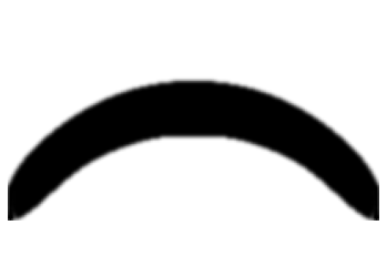
(a) Pressurized arch

(b) Pressurized piston

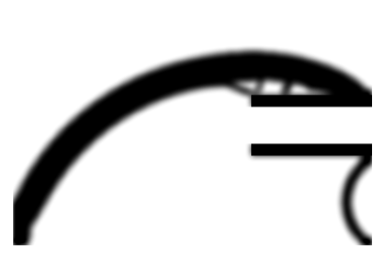
(c) Pressurized chamber

Figure 2: The optmized designs of (2(a)) Pressurized arch, (2(b)) Pressurized piston, and (2(c)) Pressurized chamber.

4 Extension to PyTOPress and optimized results

The different extensions of PyTOPress are presented herein.

4.1 Pressurized Piston

The design domain, pressure, and boundary conditions for the pressurized piston problem are adapted from [1]. To get the optimized design of the pressurized piston problem first reported in [12], we modify PyTOPress code in lines 61, 62, and 66 as follows:

⬇

PF[Bnode - 1] = 0

PF[Tnode - 1] = Pin

fixedUdofs = np.hstack([2*Bnode[math.ceil((nelx+1)/2)]-1, 2*Bnode[math.ceil((nelx+1)/2)], 2*Lnode-1, 2*Rnode-1])

To obtain the optimized result for this problem, we modify the function call on line 148 of PyTOPress as follows:

⬇

PyTOPress(300, 100, 0.20, 3, 2.4, 0.1, 8, 1, 150)

With these modifications, we obtained the optimized design for the piston problem. The result is shown in Fig. 2(b) which resembles closely with the one presented in [1].

4.2 Pressurized chamber design

The design and non-design domain, pressure, and boundary conditions for the pressurized chamber problem are adapted from [1]. To optimize the design domain, we modify the PyTOPress code by replacing lines 56 to 57 with the following code:

⬇

s1 = elNrs[(3 * nely // 8) - 1 : 17 * nely // 40, (2 * nelx // 3) - 1 : nelx]

s2 = elNrs[(23 * nely // 40) - 1 : 5*nely//8, (2 * nelx // 3) - 1 : nelx]

v1 = elNrs[(17 * nely // 40) - 1 :, (7 * nelx // 15) - 1 : 8 * nelx // 15]

v2 = elNrs[(17 * nely // 40) - 1 : 23 * nely // 40, (8 * nelx // 15) - 1 : nelx]

[NDS, NDV] = np.hstack([s1.flatten(order=’F’), s2.flatten(order=’F’)]), np.hstack([v1.flatten(order=’F’), v2.flatten(order=’F’)])

act = np.setdiff1d(np.arange(1, nel + 1), np.union1d(NDS, NDV))

s1fix = elNrs[(3 * nely // 8) - 1 : 17 * nely // 40, nelx - 1]

s2fix = elNrs[(23 * nely // 40) - 1 : 25 * nely // 40, nelx - 1]

fixx = np.unique(Pdofs[(np.hstack([s1fix.flatten(order=’F’), s2fix.flatten(order=’F’)])) - 1, :])

PF[np.hstack([Tnode - 1, Lnode - 1, Rnode - 1])] = 0

PF[np.hstack([np.unique(Pdofs[NDV - 1, :]) - 1, Bnode - 1])] = Pin

fixedUdofs = np.hstack([(2*Bnode[0]-1), (2 * Bnode[0]), (2 * Bnode[-1] - 1), (2 * Bnode[-1]), (2 * fixx - 1), (2 * fixx)])

To obtain the optimized result for this problem, we modify the function call on line 148 of PyTOPress as follows:

⬇

PyTOPress(300, 200, 0.20, 3, 6, 0.1, 10, 1, 200)

With these modifications, we get the optimized result for the pressurized chamber problem. The result is shown in Fig. 2(c) which resembles with the corresponding obtained result in [1].

5 Conclusion

In this work, we have carefully used the power of open-source libraries to convert the original MATLAB implementation. This conversion unlocks multiple benefits, making it a considerable contribution in terms of accessibility, maintainability and extensions. The Python code removes licensing obstacles and is easily accessible to a vast research community by taking advantage of Python’s open-source nature. The conversion makes use of scientific libraries like SciPy and NumPy as well as the extensive Python ecosystem. The focus is on making the code clear and concise, which improves its readability and maintainability. Python’s simple syntax helps the future development of the code in the field of TO. This opens up new possibilities for investigation and possible extensions in the Python environment in the future towards 3D problems with pressure loading [13, 14].

References

- [1] Kumar, P., 2023. TOPress: a MATLAB implementation for topology optimization of structures subjected to design-dependent pressure loads. Structural and Multidisciplinary Optimization, 66(4), p.97.
- [2] Sigmund, O. and Maute, K., 2013. Topology optimization approaches: A comparative review. Structural and multidisciplinary optimization, 48(6), pp.1031-1055.
- [3] Kumar, P., Frouws, J.S. and Langelaar, M., 2020. Topology optimization of fluidic pressure-loaded structures and compliant mechanisms using the Darcy method. Structural and Multidisciplinary Optimization, 61, pp.1637-1655.
- [4] Kumar, P., 2022. Topology optimization of stiff structures under self-weight for given volume using a smooth Heaviside function. Structural and Multidisciplinary Optimization, 65(4), p.128.
- [5] Zuo, Z.H. and Xie, Y.M., 2015. A simple and compact Python code for complex 3D topology optimization. Advances in Engineering Software, 85, pp.1-11.
- [6] Smit, T., Aage, N., Ferguson, S.J. and Helgason, B., 2021. Topology optimization using PETSc: a Python wrapper and extended functionality. Structural and Multidisciplinary Optimization, 64, pp.4343-4353.
- [7] Agarwal, A., Saxena, A. and Kumar, P., 2023. PyHexTop: a compact Python code for topology optimization using hexagonal elements. arXiv preprint arXiv:2310.01968.
- [8] Chadha, K.S., Kumar, P., 2023. PyTOaCNN: Topology optimization using an adaptive convolutional neural network in Python. arXiv preprint arXiv:2404.12244
- [9] Bruns, T.E. and Tortorelli, D.A., 2001. Topology optimization of non-linear elastic structures and compliant mechanisms. Computer methods in applied mechanics and engineering, 190(26-27), pp.3443-3459.
- [10] Svanberg, K., 1987. The method of moving asymptotes-a new method for structural optimization. International journal for numerical methods in engineering, 24(2), pp.359-373.
- [11] Kumar, P., 2023. HoneyTop90: A 90-line MATLAB code for topology optimization using honeycomb tessellation. Optimization and Engineering, 24(2), pp.1433-1460.
- [12] Bourdin, B. and Chambolle, A., 2003. Design-dependent loads in topology optimization. ESAIM: Control, Optimisation and Calculus of Variations, 9, pp.19-48.
- [13] Kumar, P. and Langelaar, M., 2021. On topology optimization of design‐dependent pressure‐loaded three‐dimensional structures and compliant mechanisms. International Journal for Numerical Methods in Engineering, 122(9), pp.2205-2220.
- [14] Kumar, P., 2024. TOPress3D: 3D topology optimization with design-dependent pressure loads in MATLAB. arXiv preprint arXiv:2405.07733 (accepted in Optimization and Engineering Journal).