Can corrections be treated in the Pomeron calculus?
Abstract
The main goal of the paper is to show that we can treat the QCD corrections in the Pomeron calculus. We develop the one dimensional model which is a simplification of the QCD approach that includes , and vertices and gives the description of the high energy interaction, both in the framework of the parton cascade and in the Pomeron calculus. In this model we show that the scattering amplitude can be written as the sum of Green’s function of -Pomeron exchanges with at . This means that choosing we can reproduce the intercepts of QCD in order. The scattering amplitude is an asymptotic series that cannot be sum using Borel approach. We found a general way of summing such series. In addition to the positive eigenvalues we found the set of negative eigenvalues which corresponds to the partonic description of the scattering amplitude. Using Abramowsky, Gribov and Kancheli cutting rules we found the multiplicity distributions of the produced dipoles as well as their entropy .
pacs:
13.60.Hb, 12.38.CyI Introduction
The question in the title of this paper arises from the rapid increase of theGreen’s function of the -BFKL Pomeron exchanges ()BFKL ; LIP ; LIREV which intercept is proportional to () as it has been shown using the BKP111BKP stands for Bartels, Kwiecinski and Praszalowicz. equation in Refs.LRS ; BART0 ; BARTU ; LLS ; LLR 222See also the short and pessimistic review of the problem in Ref.LENC .. Such an increase leads to the scattering amplitude in the BFKL Pomeron calculus being the asymptotic series of Green’s functions that cannot be summed using the Borel approach BORSUM .
The goal of this paper is to learn how to sum such asymptotic series. This problem is very old one and in the Pomeron calculus it goes under the slang name of many particle Regge poles DISASTER . For long time most experts me including believed that the asymptotic series with cannot be summed in the framework of the Pomeron calculus and we have to find a different approach. However, recently in Ref.UTMM it has been demonstrated that it is not correct. In this paper it is shown that the one dimensional model which satisfies both and channel unitarityMUSA ; BIT ; RS ; KLremark2 ; UNRFT ; UTM leads to where is the scattering amplitude of two dipoles at low energy. Nevertheless, the way to sum the asymptotic series for the scattering amplitude has been found. The method proposed in Ref.UTMM , is rather general: the analytic continuation of every to negative . After such continuation each where is rapidity. The scattering amplitude turns to the sum of the exponentially small contributions at large . On the other hand it is clear that for the intercepts proportional to this method does not work. The second feature of the model: it has infinite number of the pomeron vertices. It is not clear how this can be seen in QCD.
In this paper we consider the one dimensional model with restricted set of Pomeron vertices : , and . The parton cascade for such interactions has been developed in QCD in Ref.LELU1 . It is instructive to note that the Pomeron calculus with and corresponds to the Braun lagrangian in QCDBRAUN which reproduces the nonlinear Balitsky-Kovchegov (BK) equation in arbitrary reference frame333 As it was shown in Ref.LELU2 (see also Ref.UTM ) the BFKL cascade leads to the BK equation only in the l.r.f. with a nucleus being at the rest.. We show that this cascade generates corrections and their treatment is closely related to another unsolved theoretical problem BFKL ; LIP ; LIREV ; LELU1 ; KOLEB ; LIFT ; GLR ; GLR1 ; MUQI ; MUDI ; Salam ; NAPE ; BART ; BKP ; MV ; MUSA ; KOLE ; BRN ; BRAUN ; BK ; KOLU ; JIMWLK1 ; JIMWLK2 ; JIMWLK3 ; JIMWLK4 ; JIMWLK5 ; JIMWLK6 ; JIMWLK7 ; JIMWLK8 ; AKLL ; KOLU1 ; KOLUD ; BA05 ; SMITH ; KLW ; KLLL1 ; KLLL2 ; LEN in QCD: summation of the BFKL Pomeron loops444 The abbreviation BFKL Pomeron stands for Balitsky, Fadin, Kuraev and Lipatov Pomeron.. Indeed, in Refs.LRS ; BART0 ; BARTU ; LLS ; LLR it has been shown that the large corrections to the intercepts opf can be treated in the BFKL Pomeron calculus if we introduce the vertices of interaction of four Pomerons ().
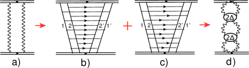 |
In this introduction we want to emphasize that the corrections have a general origin which has been discussed in seventiesDISASTER . We illustrate this origin considering the two Pomeron exchange which is shown in Fig. 1-a. This Pomeron diagram corresponds to the Feynman diagram of Fig. 1-b in which all dipoles emitted by the ladder 1 are absorbed by ladder 1’, and all dipoles produced by ladder 2 are absorbed by ladder 2’. These diagrams lead to the Green’s function of the exchange of two Pomerons: . However, the diagrams in which the dipole, emitted from ladder 1, will be absorbed by ladder 2’ are not small. We are going to call these diagrams “switch diagrams" , using the terminology suggested in Refs.LRS ; BART0 ; BARTU ; LLS ; LLR . Indeed, after first exchange ladder 1 and 2’ will give the Pomeron exchange, leading to the diagram of Fig. 1-d. Since at given rapidity we have two ‘switch diagrams: dipole emitted between ladders 1 and 2’ and the dipole emitted between ladders 2 and 1’ we can obtain the vertex , which is equal to . In QCD this vertex has suppression and we denote it as with .
The diagrams of Fig. 1-d can be summed in -representation:
| (1) |
Where is the contribution of the exchange of two Pomerons (see Fig. 1-b). Coming back to representation one can see that instead of which is expected for two Pomeron exchange. Summing diagrams of Fig. 1-e one can see that the intercept of is equal to .
II Parton cascade and Pomeron calculus
In this paper we deal with the parton cascade in which we have two micro processes: the decay of one dipole into two; and the merging of two dipoles into one.The equation for probability to have -dipoles () in this cascade have been studied in Ref.LELU2 in QCD and they have the form:
| (2) |
Eq. (II) has a simple structure: for every process of dipole splitting or merging we see two terms. The first one with the negative sign describes a decrease of probability due to the process of splitting or merging of dipoles. The second term with positive sign is responsible for the increase of the probability due to the same processes of dipole interactions.
The useful tool for discussing the structure of the parton cascade is the generating function, which has the following formMUDI ; LELU2 :
| (3) |
where is the probability to find dipoles with rapidity . For the scattering of one dipole with the target we have the following initial and boundary conditions:
| (4) |
The boundary condition follows from being probabilities.
Introducing we have a bit different equation:
| (6) |
The evolution of is generated by a non-Hermitian operator, which is
| (7) |
The BFKL Pomeron calculus is a perturbation theory around the BFKL limit of the Hamiltonian. To eЌphаsize this we rewrite the Hamiltonian of Eq. (7) as
| (8a) | |||||
| (8b) | |||||
where . Using the variable rather than is natural at weak coupling/small rapidities as it means the dipole-dipole scattering amplitude which is small in this regime. Fig. 2 shows the first Pomeron diagrams for the dipole-dipole scattering. One can see that integrations over and reduce the diagram of Fig. 2-b to the zero order contribution to and to with a different intercept in comparison with Fig. 2-a.
It is instructive to calculate the diagramm of Fig. 2-b using the representation:
| (9) |
In this representation the contribution of Fig. 2-b has the fornm
| (10) | |||||
The first contribution to leads to the renormalization of the vertices of interaction with dipoles in Fig. 2-a. The second one is responsible for the new intercept of .
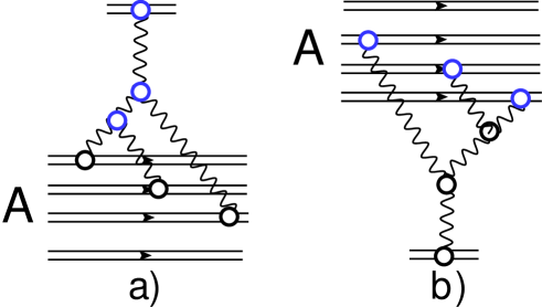
The hamiltonian of Eq. (8a) has several attractive features:(i) for it coincides with the Braun hamiltonian for the Pomeron calculus in QCDBRAUN ; (ii) it gives Balitsky-Kovchegov nonlinear equation in wide range of energy and describe dipole nucleus interaction both in the lab.r.f and in the frame where a nucleus is a fast moving projectile (see Fig. 3); and it preserves the probabilistic interpretation of the scattering amplitude given by Mueller and Salam MUSA .
The Pomeron calculus with the hamiltonian of Eq. (8a) as well as any other Pomeron calculus satisfies the t-channel unitarity. However we have problem with s-channel unitarity as has been discussed in Ref.UNRFT (see section four of this paper).
III Eigenfunctions of the hamiltonian
Eq. (6) can be rewritten as the equation for the eigenfunction of hamiltonian of Eq. (7) in the representation of Eq. (9):
| (11) |
Since our hamiltonian is non-hermitian but with real eigenvalues we have two sets of eigenfunctions: with negative eigenvalues and with positive eigenvalues . This reflects the two way of describing the scattering amplitude. The first way is the parton model in which the scattering amplitude in the lab.r.f. isMUSA
| (12) |
In Eq. (12) we consider the scattering with a dipole and we interpret as the scattering two dipoles amplitude at low energies (se Fig. 3). is the coefficient which we need to find from the initial conditions of Eq. (4).
On the other had we have a different way to describe the scattering amplitude using the factorial moments
| (13) |
In the moments representation the scattering amplitude takes the form (see for example Ref.LELU2 ):
| (14) |
Again is the coefficient which we need to find from the initial conditions of Eq. (4). Series of Eq. (14) emerges in the Pomeron calculus with . This series is basically an asymptotic series which we need to sum. The result of summation should give the analytic function given by Eq. (12).
For our cascade coincides with the BFKL cascade and in Ref.UTMM both sets of eigenfunction have been found. It turns out that
| (15) |
with the corresponding eigenvalues and . Eq. (12) take the following form for the BFKL cascade:
| (16) |
is the interaction of two dipoles at low energies. Note, that for we have to introduce this amplitude (see for example Fig. 3-a) . We need to keep at to have dipole nucleus scattering in this case.
For Eq. (14) we have:
| (17) |
We got the same answers for two series. However, series of Eq. (17) is asymptotic one at large which has been summed using Borel resummation procedure, while Eq. (16) is an absolutely converged series at large . It is instructive to note at small gives the contribution of the exchange of one Pomeron while the series of Eq. (16) has to be resummed.
III.1 Eigenfunction for negative eigenvalues
The Sturm- Liouville equation of Eq. (18) has the following general featuresKOLEV ; POLY :
-
1.
It has infinite set of eigenvalues , which monotonically increase with . In our case of Eq. (18) all .
-
2.
The multiplicity of each eigenvalue is equal to 1.
-
3.
The eigenfunctions are orthogonal
(20) -
4.
For large
(21) -
5.
For our equation
(22) leading to
(23) -
6.
An arbitrary function F(u), that has a continuous derivative and satisfies the boundary conditions of the Sturm-Liouville problem (in other words, a function that we, as physicists, want to find), can be expanded into absolute and uniformly convergent series in eigenfunctions:
(24) -
7.
For takes the form:
(25)
Therefore, one can see that we know a lot about which corresponds to the negative eigenvalues. In Ref.KOLEV are found for the arbitrary values of . This solution is
| (26) |
with . is the prolate spheroidal wave function with the fixed order parameter and arbitrary degree parameter which is an integer, (see Refs. ABST ; SPHF ), namely,
| (27) |
Eq. (18) gives the following parameters of Eq. (27):
| (28) |
For large while for small (see Ref.ABST formulae 21.6.2 and 21.7.6).
III.2 for
In this subsection we are going to find of Eq. (9) for small . We hope to obtain a simpler set of the eigenvalues and eigenfunctions that in a general case that has been considered in the previous section. Second, we expect a transparent relation between these eigenvalues and the positive eigenvalues that we will consider in the next subsection.
In the omega representation of Eq. (9) the set of equations of Eq. (II) takes the following form, taking into account Eq. (4):
| (29a) | |||
| (29b) | |||
| (29c) | |||
| (29d) | |||
| (29e) | |||
Note that the r.h.s., of Eq. (29a) comes from the initial condition of Eq. (4).
Plugging Eq. (29b) into Eq. (29a) we obtain:
| (30) |
Solution to Eq. (30) has the form for small values of :
| (31) |
For from Eq. (29a) and Eq. (29b) we have
| (32) |
At we see that
| (33) |
which gives . In other word both and diagonalize the matrix of . The general expression for is
| (34) |
Eq. (32) leads to
| (35) |
if we plug in this equation from Eq. (29c).
From the general Eq. (29e) we can get the following equation555 In the next section we will give the more expanded discussions how to get such an equation. for
| (36) |
III.3 Positive eigenvalues
We are going to find the positive eigenvalues by writing the equations for the factorial moments of Eq. (13) using that (e.g. see Ref.LELU2 )
| (37) |
Differentiating Eq. (6) we obtain
| (38a) | |||||
| (38b) | |||||
| (38c) | |||||
| (38d) | |||||
| (38e) | |||||
| (38f) | |||||
| (38g) | |||||
For we have the equations for the moments in the BFKL parton cascade. Solutions for this case are known(e.g. Ref.KHLE ):
| (39) |
The representation is defined in Eq. (9). Recall that the exchange of the BFKL Pomeron is with our definition of .
The set of power moments diagonalizes Eq. (38a) - Eq. (38g). Each of them is equal to or in representation. On the other hand
| (40) |
Now we attempt to solve Eq. (38a) - Eq. (38g), considering . First, we rewrite these equations in representation (see Eq. (9)). Eq. (38a) and Eq. (38b) takes the form:
| (41a) | |||
| (41b) | |||
Note that the r.h.s., of Eq. (41a) comes from the initial condition of Eq. (4). Plugging from the second equation we obtain:
| (42) |
Neglecting corrections of size, one can see that solving Eq. (42) we obtain:
| (43) |
It is easy to see that Eq. (43) corresponds to the third contribution of Fig. 2-b in the Pomeron calculus. Summing Eq. (41a) and Eq. (41b) we obtain the following equation for :
| (44) |
Plugging in this equation from Eq. (38c) ;
| (45) |
we have
| (46) |
In the vicinity of Eq. (47) takes the form:
| (47) |
The calculations of Eq. (10) -type shows that sum of the Pomeron diagrams of Fig. 4 leads to Eq. (47).
We need to sum Eq. (38a)-Eq. (38c) for finding and express from Eq. (38d) neglecting terms proportional to . The resulting equation takes the form:
| (48) |
which leads to
| (49) |
We can easily calculate the intercept for using Eq. (38e)- Eq. (38g). From Eq. (40) one can see that . Multiplying Eq. (38e) by and adding to Eq. (38f) we obtain:
| (50) |
which leads to
| (51) | |||||
where we put in the second equation. From this equation one can see that we obtain the positive eigenvalues which are equal to
| (52) |
For finding the contribution in Eq. (50) we use from Eq. (40). The equation for takes the form:
| (53) |
where are binomial coefficients.
Plugging in this equation from Eq. (38g) we obtain
| (54) | |||||
Neglecting terms that are proportional to we can use Eq. (39) for . Summing over we obtain:
| (55) |
Note, that Eq. (55) describe , and calculated above.
IV Scattering amplitude
IV.1 Sum of decreasing exponents
First we consider the representation of given by Eq. (12), viz.:
| (57) |
where are given by Eq. (26). We need first to find the asymptotic solution to Eq. (6) which does not depend on and has the following boundary conditions:
| (58) |
One can see that
| (59) |
has the following initial conditions:
| (60) |
Therefore,
| (61) |
where
| (62) |
IV.2 Pomeron calculus
From Eq. (37) one can see that
| (63) |
However, it is more convenient for us to use the expression for the scattering amplitude which follows directly from Eq. (12):
| (64) |
Plugging Eq. (55) into this equation we have
| (65) |
Eq. (65) is the series of the Green’s function of the many Pomerons exchanges each of which is equal to .
This series is not only asymptotic one but it cannot be summed using Borel approach. Actually in Ref.UTMM it is proposed the way how to sum such series (see appendix A of this paper). The prescription is to replace by
| (66) |
Plugging into Eq. (65) this representation we reduce the series to the Borel summed one. Indeed, Eq. (65) takes the form:
| (67) |
Summing over we obtain
| (68) |
with .
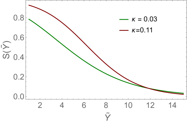
In Fig. 5 we plot versus at two different values of , which we will discuss below. One can see that decreases at large certifying that our way of resummation of the asymptotic series gives the analytic function that describes the scattering amplitude.
At large Eq. (68) leads to
| (69) |
IV.3 The value of .
We have learnt three lessons. First, the Pomeron calculus with the hamiltonian of Eq. (8a) leads to the intercepts for n Pomeron exchanges which are . Second, we found the way to sum the asymptotic series for the scattering amplitude and, third, this amplitude shows the saturation at high energies ().
As we have mentioned the hamiltonian of Eq. (8a) without vertex (see Eq. (8b)) is the one dimensional version of the Braun hamiltonian in QCD BRAUN . This hamiltonian is the minimum that we need to get the BK equation to be valid for the deep inelastic scattering in the Bjorken frame in which the virtual photon is at the rest. Note that the first nonlinear equation which coincides with the BK one in the momentum representation, was derived in this frameGLR . In the framework of this approach vertex from the additional requirement that the hamiltonian will describe the parton cascade (see Ref.LELU2 ). In such interpretation corresponds to the QCD vertex which is proportional to . Hence . In Fig. 5 we take .
However, the most interesting case for us in this paper is to interpret the hamiltonian of Eq. (8a) in a different way.Indeed, the term with vertex appears in QCD when we calculate the corrections, as we have argued in the introduction. In QCD these corrections generate of the order of . Hence we come to the hamiltonian of Eq. (8a) as the way to generate the parton cascade in order of QCD. is the natural estimates for this approach.
Bearing this in mind we can conclude that the hamiltonian of Eq. (8a) shows that correction in QCD can be summed in the framework of the Pomeron calculus.
V Multiplicity distributions and entropy of produced dipoles.
The presentation of the scattering matrix in the form of Eq. (65) and Eq. (67) is very convenient for use of the AGK cutting rulesAGK for determining the multiplicity distributions of produced dipoles, since each term of the series is the exchange of Pomerons:
| (70) |
The AGK cutting rules AGK allows us to calculate the contributions of -cut Pomerons if we know : the contribution of the exchange of -Pomerons to the cross section. They take the form:
| (71a) | |||||
| (71b) | |||||
| (71c) | |||||
where is the total cross section and denotes the cross section with the multiplicity of produced dipoles which is much less than . In other words, it is the cross section of the diffraction production.
The total production of cut Pomrerons is equal to
| (72) |
.
The main idea of using the AGK cutting rules is originated from the contribution of the BFKL Pomeon and s-channel unitarity for its Gree’s function:
| (73) |
where is the cross section of the produced dipoles with the average number, with is the intercept of . The multiplicity distribution of these dipoles is the Poisson one, viz.:
| (74) |
Let us consider for simplicity the first term in . For it takes the following form:
| (77) |
Integral over can be taken using the method of steepest descent with the following equation for the saddle point
| (78) |
This equation can be rewritten as W-Lambert equation:
| (79) |
with the solution: where is the W-Lambert function (see section 4.13 of Ref.OLBC ). This function can be written as the following series:
| (80) |
 |
 |
 |
| Fig. 6-a | Fig. 6-b | Fig. 6-c |
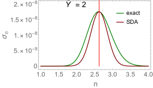
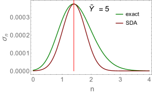
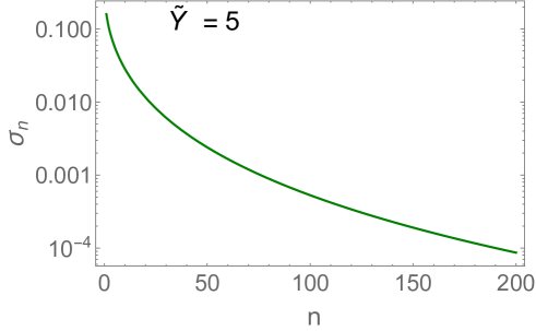
Fig. 6 shows that the correctly determine the maximum of the function but the method of steepest descent leads to more narrow distribution. For small one can see from Eq. (80) that . In Fig. 7 we plot for . One can see this kind of the behaviour.
 |
 |
| Fig. 7-a | Fig. 7-b |
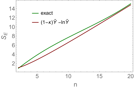
In Fig. 7-b we plot the calculation of the entropy of the produced dipoles:
| (81) |
We compare this calculations with . This expression is close to the prediction of Ref.KHLE but strictly speaking this paper predicts . Therefore, we can see that the contribution of the enhanced Pomeron diagrams manifest themselves differently in and .
VI Conclusions
The main result of the paper is that we show that the Pomeron calculus can be used to treat the corrections in QCD. In the one dimensional model which is a simplification of the QCD approach LELU1 that gives the description of the high energy interaction both in the framework of the parton cascade (see Refs.MUDI ; MUSA for details) and in the Pomeron calculus, we found the following. First, the scattering amplitude can be written as the sum of Green’s function of -Pomeron exchanges with at . This means that choosing we can reproduce the intercepts of QCD in order. Second, the scattering amplitude is an asymptotic series that cannot be sum using Borel approach. We found the general way of summing such series (see Eq. (67)). Third, we found the set of negative eigenvalues which corresponds to the partonic description of the scattering amplitude. Fourth, it turns out that the negative eigenvalues at are equal to (see Eq. (56)). Therefore, we can view the expansion of the scattering amplitude in the eigenfunctions with negative eigenvalues as the analytic continuation of the Pomeron calculus to the negative . Hence, we generalize the analysis of the BFKL and UTM model, given in Ref.UTMM , to our approach. Fifth, using AGK AGK cutting rules we found the multiplicity distributions of the produced dipoles as well as their entropy . At large . This expression is close to the prediction of Ref.KHLE : , where is the average multiplicity. However, we show that at large . Therefore, we found that the enhanced diagrams of the Pomeron calculus contribute in a different way to and the entropy.
As we have discussed in the introduction both the QCD hamiltonian of Eq. (7)-type LELU1 as well as the one dimensional incarnation of it (see Eq. (8a)) satisfy the t-channel but have problems with the s-channel unitarities. It is enough to mention that hamiltonian of Eq. (8a) is quite different with the “diamond" hamiltonian KLLL2 which is the best that we know in QCD. However, we do not see how the correct QCD hamiltonian can change two features of the model: the intercepts , which is found in QCD and our way of summing the asymptotic series with such kind of intercepts.
Acknowledgements
We thank our colleagues at Tel Aviv university for encouraging discussions. Special thanks go A. Kovner, M. Li and M. Lublinsky for stimulating and encouraging discussions on the subject of this paper. This research was supported by Binational Science Foundation grant #2022132.
References
- (1) V. S. Fadin, E. A. Kuraev and L. N. Lipatov, Phys. Lett. B60, 50 (1975); E. A. Kuraev, L. N. Lipatov and V. S. Fadin, Sov. Phys. JETP 45, 199 (1977), [Zh. Eksp. Teor. Fiz.72,377(1977)]; I. I. Balitsky and L. N. Lipatov, Sov. J. Nucl. Phys. 28, 822 (1978), [Yad. Fiz.28,1597(1978)].
- (2) L. N. Lipatov, Sov. Phys. JETP 63, 904 (1986) [Zh. Eksp. Teor. Fiz. 90, 1536 (1986)].
- (3) L. N. Lipatov, Phys. Rept. 286 (1997) 131.
- (4) J. Bartels, Nucl. Phys. B 175 (1980), 365-401 J. Kwiecinski and M. Praszalowicz, Phys. Lett. B 94 (1980), 413-416
- (5) E. M. Levin, M. G. Ryskin and A. G. Shuvaev, Nucl. Phys. B 387, 589-616 (1992) doi:10.1016/0550-3213(92)90208-S
- (6) J. Bartels, Phys. Lett. B 298, 204-210 (1993) doi:10.1016/0370-2693(93)91731-2
- (7) J. Bartels, Z. Phys. C 60, 471-488 (1993) doi:10.1007/BF01560045
- (8) E. Laenen, E. Levin and A. G. Shuvaev, Nucl. Phys. B 419, 39-58 (1994) doi:10.1016/0550-3213(94)90356-5 [arXiv:hep-ph/9308294 [hep-ph]].
- (9) E. Laenen and E. Levin, Ann. Rev. Nucl. Part. Sci. 44, 199-246 (1994) doi:10.1146/annurev.ns.44.120194.001215
- (10) E. Levin, Eur. Phys. J. C 83 (2023) no.5, 452 doi:10.1140/epjc/s10052-023-11638-0 [arXiv:2301.09337 [hep-ph]].
-
(11)
Bruce Shawyer and Bruce Watson, “Borel’s Method of Summability, Theory and Application” , Clarendon Press, Oxford,1994;
Ovidiu Costin,“Asymptotocs and Borel Summability”, Chapman & HALL/CRC Monographs and Surveys in Pure and Applied Mathematics, CRC Press, Taylor & Frencis Group,2009;
. - (12) S.G. Matinyan and A.G. Sedrakyan, JETP Lett. 23 (1976) 588; 24 (1976) 240; Soy. J. NucI. Phys. 24 (1976) 844; B.M. Mc Coy and T.T. Wu, Phys. Rev. D12 (1975) 546, 577
- (13) A. Kovner, E. Levin and M. Lublinsky, “High energy scattering in the Unitary Toy Model,” [arXiv:2406.12691 [hep-ph]].
- (14) A. H. Mueller and G. P. Salam, Nucl. Phys. B 475, 293 (1996), [hep-ph/9605302]; G. P. Salam, Nucl. Phys. B 461, 512 (1996), [hep-ph/9509353].
- (15) J.-P. Blaizot, E. Iancu and D. N. Triantafyllopoulos, Nucl. Phys. A 784 (2007) 227.
- (16) P. Rembiesa and A. M. Stasto, Nucl. Phys. B 725 (2005) 251.
- (17) A. Kovner and M. Lublinsky, Nucl. Phys. A 767 171 (2006).
- (18) A. Kovner, E. Levin and M. Lublinsky, JHEP 08 (2016), 031.
- (19) A. Kovner, E. Levin and M. Lublinsky, JHEP 05, 019 (2022) doi:10.1007/JHEP05(2022)019 [arXiv:2201.01551 [hep-ph]].
- (20) E. Levin and M. Lublinsky, Nucl. Phys. A 763 (2005), 172-196 doi:10.1016/j.nuclphysa.2005.08.021 [arXiv:hep-ph/0501173 [hep-ph]].
- (21) M. A. Braun, Phys. Lett. B 483, 115 (2000), Eur. Phys. J. C 33, 113 (2004); Phys. Lett. B 632, 297 (200
- (22) E. Levin and M. Lublinsky, Phys. Lett. B 607 (2005) 131; Nucl. Phys. A 763 (2005) 172.
- (23) Yuri V. Kovchegov and Eugene Levin, “ Quantum Chromodynamics at High Energies", Cambridge Monographs on Particle Physics, Nuclear Physics and Cosmology, Cambridge University Press, 2012 .
-
(24)
L. N. Lipatov,
Nucl. Phys. B 365, 614 (1991),
Nucl. Phys. B 452, 369 (1995),
R. Kirschner, L. N. Lipatov and L. Szymanowski, Nucl. Phys. B 425, 579 (1994), Phys. Rev. D 51, 838 (1995). - (25) L. V. Gribov, E. M. Levin and M. G. Ryskin, Phys. Rept. 100, 1 (1983).
- (26) E. M. Levin and M. G. Ryskin, Phys. Rept. 189, 267 (1990).
- (27) A. H. Mueller and J. Qiu, Nucl. Phys. B268 (1986) 427.
-
(28)
A. H. Mueller,
Nucl. Phys. B 415 (1994) 373;
Nucl. Phys. B 437 (1995) 107;
A. H. Mueller and B. Patel, Nucl. Phys. B 425, 471, 1994. - (29) G. P. Salam, Nucl. Phys. B 461, 512 (1996); [hep-ph/9509353].
- (30) H. Navelet and R. B. Peschanski, Nucl. Phys. B 507 (1997), 353-366 [arXiv:hep-ph/9703238 [hep-ph]].
- (31) J. Bartels, Z. Phys. C 60 (1993), 471-488 ; J. Bartels and M. Wusthoff, Z. Phys. C 66 (1995), 157-1801; J. Bartels and C. Ewerz, JHEP 09 (1999), 026 [arXiv:hep-ph/9908454 [hep-ph]]; C. Ewerz, JHEP 0104 (2001) 031.
-
(32)
J. Bartels,
Nucl. Phys. B175, 365 (1980);
J. Kwiecinski and M. Praszalowicz, Phys. Lett. B94, 413 (1980). - (33) L. McLerran and R. Venugopalan, Phys. Rev. D49 (1994) 2233, Phys. Rev. D49 (1994), 3352; D50 (1994) 2225; D59 (1999) 09400.
- (34) Y. V. Kovchegov and E. Levin, Nucl. Phys. B 577 (2000) 221.
-
(35)
M. A. Braun,
Eur. Phys. J. C16 (2000) 337;
M. A. Braun and G. P. Vacca, Eur. Phys. J. C6 (1999) 147;
J. Bartels, M. Braun and G. P. Vacca, Eur. Phys. J. C 40, 419 (2005).
J. Bartels, L. N. Lipatov and G. P. Vacca, Nucl. Phys. B 706, 391 (2005). - (36) I. Balitsky, Phys. Rev. D60, 014020 (1999); Y. V. Kovchegov, Phys. Rev. D60, 034008 (1999).
- (37) A. Kovner and M. Lublinsky, JHEP 02 (2007), 058 [arXiv:hep-ph/0512316 [hep-ph]].
- (38) J. Jalilian-Marian, A. Kovner, A. Leonidov, and H. Weigert, , Nucl. Phys. B504 (1997) 415–431, [ arXiv:hep-ph/9701284].
- (39) J. Jalilian-Marian, A. Kovner, A. Leonidov, and H. Weigert, , Phys.Rev. D59 (1998) 014014, [arXiv:hep-ph/9706377 [hep-ph]].
- (40) A. Kovner, J. G. Milhano, and H. Weigert, , Phys. Rev. D62 (2000) 114005, [ arXiv:hep-ph/0004014].
- (41) E. Iancu, A. Leonidov, and L. D. McLerran, ,Nucl. Phys. A692 (2001) 583–645, [ arXiv:hep-ph/0011241].
- (42) E. Iancu, A. Leonidov, and L. D. McLerran, , Phys. Lett. B510 (2001) 133–144, [ arXiv:hep-ph/0102009].
- (43) E. Ferreiro, E. Iancu, A. Leonidov, and L. McLerran, , Nucl. Phys. A703 (2002) 489–538, [ arXiv:hep-ph/0109115].
- (44) H. Weigert, Nucl. Phys. A 703 (2002), 823-860 [arXiv:hep-ph/0004044 [hep-ph]].
- (45) A. Kovner and J. G. Milhano, Phys. Rev. D 61 (2000), 014012 [arXiv:hep-ph/9904420 [hep-ph]].
- (46) T. Altinoluk, A. Kovner, E. Levin and M. Lublinsky, JHEP 04 (2014), 075 [arXiv:1401.7431 [hep-ph]].
- (47) A. Kovner and M. Lublinsky, Phys. Rev. D 71 (2005), 085004 [arXiv:hep-ph/0501198 [hep-ph]].
- (48) A. Kovner and M. Lublinsky, Phys. Rev. Lett. 94, 181603 (2005), [hep-ph/0502119].
- (49) I. Balitsky, Phys. Rev. D 72, 074027 (2005), arXiv:hep-ph/0507237.
- (50) Y. Hatta, E. Iancu, L. McLerran, A. Stasto and D. N. Triantafyllopoulos, Nucl. Phys. A 764, 423 (2006).,arXiv:hep-ph/0504182.
- (51) A. Kovner, M. Lublinsky and U. Wiedemann, JHEP 06 (2007), 075 [arXiv:0705.1713 [hep-ph]]; T. Altinoluk, A. Kovner, M. Lublinsky and J. Peressutti, JHEP 0903, 109 (2009), [arXiv:0901.2559 [hep-ph]].
- (52) A. Kovner, E. Levin, M. Li and M. Lublinsky, JHEP 09 (2020), 199 [arXiv:2006.15126 [hep-ph]].
- (53) A. Kovner, E. Levin, M. Li and M. Lublinsky, JHEP 10 (2020), 185 [arXiv:2007.12132 [hep-ph]].
- (54) E. Levin, [arXiv:2209.07095 [hep-ph]].
- (55) Andrey D. Polyanin, “Handbook of Linear Differential Equations For Engineers and Scientists", Chapman & Hall/CRC, 2002
- (56) M. Kozlov and E. Levin, Nucl. Phys. A 779 (2006) 142.
- (57) M.Abramowitz and Stegun,“Handbook ofMathematical Functions", Dover Publicartion,Inc. New York,1972.
-
(58)
Le-Wei Li, Xiao-Kang Kang, Mook-Seng Leong,“Spheroidal Wave Functions in Electromagnetic Theory ",L Jon Wiley & Son Inc. 2002.
P.Falloon,“Homepage of the Spheroidal Wave Functions", ; - (59) D. E. Kharzeev and E. M. Levin, Phys. Rev. D 95 (2017) no.11, 114008 doi:10.1103/PhysRevD.95.114008 [arXiv:1702.03489 [hep-ph]].
- (60) V. A. Abramovsky, V. N. Gribov and O. V. Kancheli, Yad. Fiz. 18 (1973), 595, (Sov.J. Nucl.Phys. 18 (1974),308);
- (61) F.Olver, D. Lozier, R.Boisvert and C. Clark, eds.“NIST handbook of Mathematical Functions". U.S. Departament of Commerce, National Institute of Standard and Technology, Cambridge University Press, Wasington, DC, Cambridge, 2010