Unlearning as multi-task optimization: A normalized gradient difference approach with an adaptive learning rate

Abstract

Machine unlearning has been used to remove unwanted knowledge acquired by large language models (LLMs). In this paper, we examine machine unlearning from an optimization perspective, framing it as a regularized multi-task optimization problem, where one task optimizes a forgetting objective and another optimizes the model performance. In particular, we introduce a normalized gradient difference (NGDiff) algorithm, enabling us to have better control over the trade-off between the objectives, while integrating a new, automatic learning rate scheduler. We provide a theoretical analysis and empirically demonstrate the superior performance of NGDiff among state-of-the-art unlearning methods on the TOFU and MUSE datasets while exhibiting stable training.

1 Introduction

Large language models (LLMs) consume a large amount of data during pre-training. After the model is built, we may have to unlearn certain data points that contain potentially sensitive, harmful, or copyrighted content. As re-training from scratch in such a case is not feasible due to the associated costs, researchers have developed a number of machine unlearning methods applied after training.

Existing machine unlearning methods are formulated primarily as minimizing memorization through the language model loss [22, 7, 34]. In particular, the Gradient Ascent (GA) method maximizes the language model (LM) loss (i.e., minimizes the negative LM loss) on the target forget set (F). However, this approach can also negatively affect the utility of the model. To mitigate the utility loss, the Gradient Difference (GDiff) method selects a subset of the training data as the retain set (R), minimizing the sum of the negative LM loss on the forgetting set and the standard LM loss on the retaining set. This approach has been empirically shown to effectively preserve the model’s performance [31, 36]. Similarly, Negative Preference Optimization (NPO) [55] assigns a lower likelihood of forgetting data, thereby balancing the unlearning performance with model utility.

Despite these successes, there are still two key issues preventing the methods from reaching their full potential. First, balancing retaining and forgetting losses is difficult (Figure 1) given the disproportionate sizes of the forget and retain datasets. Second, the optimization methods for unlearning are usually sensitive to the learning rate (cf., Appendix A, Figure 6). For instance, various learning rates can lead to substantial changes in the ROUGE scores and loss values even for the same algorithm, making the unlearning methods unstable and difficult to use in practice.

In this paper, we carefully examine unlearning from an optimization perspective and formulate it as a multi-task optimization (MTO) problem [9, 51]: we aim to minimize the LM loss (i.e., maximize the utility) on the retaining set and maximize the LM loss on the forgetting set (i.e., minimize memorization), simultaneously. To solve this two-task problem, we study the rich literature of multi-task methods that seeks the Pareto optimality of two tasks (e.g., IMTL [33], GradNorm [10], RLW [30], PCGrad [52], and scalarization [3]), and design an approach specifically for the LLM unlearning problem.

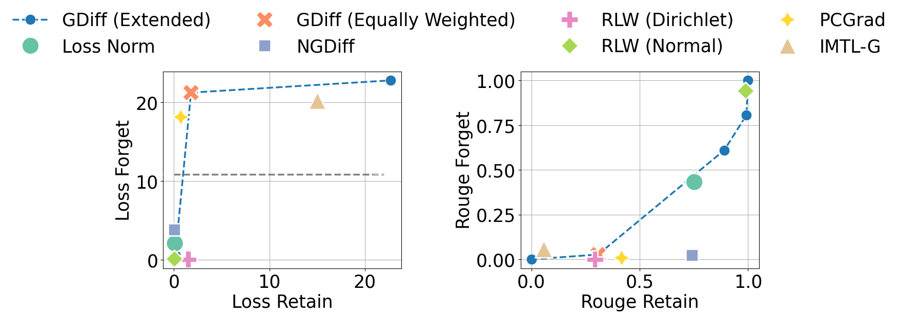
Figure 1: Loss values and ROUGE scores on the forgetting and retaining data from the TOFU dataset using different unlearning methods on the Phi-1.5 language model. We apply the extended GDiff with various coefficients (see (3), $0\leq c\leq 1$) and connect the results with a blue dashed line. We denote MTO methods as different markers, and use a grey dashed line to represent the loss of random guess.

Inspired by the simplicity and strong empirical performance of linear scalarization methods, which minimize a linearly weighted average of task losses, we propose an LLM unlearning method, NGDiff, based on dynamic scalarization, and analyze its theoretical properties. Building on the analysis, we introduce an automatic learning rate adaptation method tailored for LLM unlearning.

We showcase the effectiveness of our method through extensive experiments on multiple datasets, different LLMs and vision models. For example, on TOFU [36], NGDiff achieves 40% higher model utility while maintaining comparable unlearning performance with Llama2-7B. Figure 1 highlights the effectiveness of NGDiff.

Contributions are summarized as follows:

• We formalize LLM unlearning as a multi-task optimization problem and unify the terminology used across both fields. We demonstrate the Pareto optimality for scalarization-based unlearning methods under some assumptions.

• Through the lens of multi-task optimization, we propose a novel unlearning method NGDiff for LLM unlearning, which uses the gradient norms to dynamically balance the forget and retain tasks. NGDiff improves both tasks simultaneously and monotonically with a proper learning rate scheduling.

• We integrate NGDiff with GeN [4], which uses Hessian-based learning rate selection for stable convergence.

2 Related Work

We position our work within the related literature. More discussion and background on learning rate-free techniques are in Appendix E.

LLM unlearning The extensive data used in training LLMs raises significant concerns. Certain data sources contain personal information [5], outdated knowledge [50], and copyright-protected materials [45]. In addition, adversarial data attacks can maliciously manipulate training data to embed harmful information [48, 27].

To remove unwanted information without retraining the entire model, machine unlearning has been proposed using techniques such as data slicing [2], influence functions [47], and differential privacy [18]. However, these methods are challenging to scale to LLMs due to their complexity. Recently, efficient approximate unlearning methods have been proposed for LLMs [17, 54, 22, 39, 6]. They mostly focus on designing unlearning objectives or hiding unwanted information. However, none addresses the fundamental optimization problem. Our paper bridges this gap and complements existing approaches. Further discussion of the challenges surrounding LLM unlearning can be found in benchmarks [43, 36] and surveys [44, 35].

Note that the literature on knowledge editing [13] is also relevant. However, model editing typically focuses on surgically updating LLMs for specific knowledge, whereas unlearning removes the influence of particular documents. The techniques presented in this paper could potentially be applied to knowledge editing.

Multi-task optimization In NLP, multi-task learning [56] typically refers to building a model that can perform well on multiple tasks simultaneously by sharing representations, introducing constraints, or combining multiple learning objectives. Multi-task optimization, on the other hand, focuses on a slightly different concept – optimizing two distinct learning objectives simultaneously. The key challenge is how to balance the trade-off among objectives during the optimization procedure by modifying the per-task gradients (e.g. PCGrad [52], RLW [30], IMTL [33]). Several recent works have studied Pareto frontier and optimally in context of NLP tasks (e.g., multi-lingual machine translation [8, 51] and NLP fairness [19]). While optimization is often treated as a black-box tool in NLP research, studying optimization provides deeper insights and inspires new algorithms.

3 Unlearning as multi-task optimization

This section casts machine unlearning as a multi-task optimization (MTO), specifically the two-task optimization problem. Let the retain set be denoted by R and the forget set by F, with $L_{\textup{R}}$ and $L_{\textup{F}}$ representing the corresponding cross-entropy losses for language modeling. We are interested in finding

$$\arg\min\nolimits_{\theta}L_{\textup{R}}(\bm{\theta})\quad\cap\quad\arg\max\nolimits_{\theta}L_{\textup{F}}(\bm{\theta}),$$ (1)

where $\bm{\theta}$ represents the model parameters.

There might not be a solution that simultaneously achieves both objectives in Eq. (1). For LLMs, the unlearning solutions generally exhibit a trade-off between performance in R and F (cf., Figure 1). To forget F, one may unavoidably unlearn general knowledge such as grammar rules on F, which can sacrifice the performance on R.

In MTO, Pareto optimality is used to characterize the trade-offs between multiple objectives. In layperson’s terms, if $\theta$ is Pareto optimal, it is impossible to improve $L_{\textup{R}}$ or $L_{\textup{F}}$ without worsening the other. Formal definition is in below:

Definition 1 (Pareto optimality in unlearning).

For two models $\bm{\theta}$ and $\bm{\theta}^{\prime}$, if $L_{\textup{R}}(\bm{\theta})\geq L_{\textup{R}}(\bm{\theta}^{\prime})$ and $L_{\textup{F}}(\bm{\theta})\leq L_{\textup{F}}(\bm{\theta}^{\prime})$ with at least one inequality being strict, then $\bm{\theta}$ is dominated by $\bm{\theta}^{\prime}$. A model is Pareto optimal if it is not dominated by any other models.

In the remainder of this section, we will discuss current unlearning methods in a unified MTO framework and analyze their Pareto optimality. Building on this, we then propose a dynamic scalarization approach tailored to LLM unlearning.

3.1 Static linear scalarization

A popular MTO method is scalarization, which addresses MTO by optimizing the linear scalarization problem (LSP). This method combines multiple tasks into a single, reweighted task:

$$\textup{LSP}(\bm{\theta};c)=c\cdot L_{\textup{R}}(\bm{\theta})-(1-c)\cdot L_{\textup{F}}(\bm{\theta}),$$ (2)

where $c$ is fixed. At iteration $t$, the gradient of LSP, $\bm{g}_{\text{static}}(\bm{\theta}_{t};c)$, lies within the linear span of per-task gradients as shown in Figure 2 (yellow area):

$$\bm{g}_{\text{static}}(\bm{\theta}_{t};c)=\frac{\partial\textup{LSP}}{\partial\bm{\theta}_{t}}=c\cdot\bm{g}_{\textup{R}}(\bm{\theta}_{t})-(1-c)\cdot\bm{g}_{\textup{F}}(\bm{\theta}_{t}).$$ (3)

Then, the corresponding update rule by the (stochastic) gradient method is

$$\bm{\theta}_{t+1}=\bm{\theta}_{t}-\eta_{t}[c\cdot\bm{g}_{\textup{R}}(\bm{\theta}_{t})-(1-c)\cdot\bm{g}_{\textup{F}}(\bm{\theta}_{t})].$$ (4)

Remark 3.1.

We term the static linear scalarization as the extended GDiff in this work. Some existing methods are special cases of extended GDiff. For example, Gradient Descent (GD) on retaining set is equivalent to extended GDiff with $c=1$. Gradient Ascent (GA) on forgetting is equivalent to that with $c=0$, and vanilla GDiff [31] set $c=0.5$ (i.e., equally weighted).

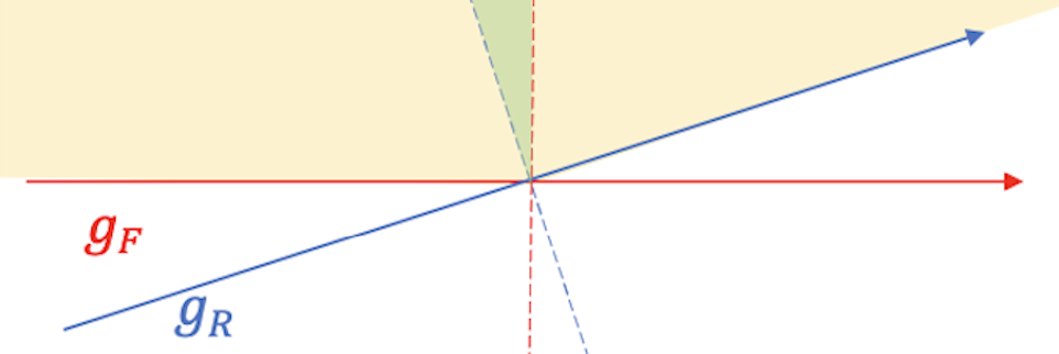
Figure 2: Gradient space in 2-dimension. $\color[rgb]{1,0,0}\bm{g}_{\textup{F}}$ is the forgetting gradient and $\color[rgb]{0,0,1}\bm{g}_{\textup{R}}$ is the retaining gradient, each with a perpendicular dashed line. Yellow area is the linear span (Eq. (3)) by scalarization. Green area is positively correlated to $\bm{g}_{\textup{R}}$ and negatively correlated to $\bm{g}_{\textup{F}}$ by Eq. (7), whereas NGDiff always stays within this green area at each iteration.

A nice property of linear scalarization is the Pareto optimality at the convergence of models, which we state in Lemma 2 (proof in Appendix G) for the static $c$ and later extend to Theorem 3 for the dynamic $c_{t}$ in Section 3.2.

Lemma 2 (restated from [51]).

For any $0<c<1$, the model $\bm{\theta}^{*}_{\text{LSP}}(c)\in\operatorname*{arg\,min}_{\theta}\textup{LSP}(\bm{\theta};c)$ is Pareto optimal.

Lemma 2 suggests that we can sweep through $c\in[0,1]$ and construct the Pareto frontier after sufficiently long training time (e.g., the blue dotted line in Figure 1). However, while any $c$ leads to a Pareto optimal point, the solution may be useless: e.g., perfect memorization on $(\textup{R},\textup{F})$ that fails to unlearn is also Pareto optimal. Next, we investigate different choices of c by extending the static scalarization in (3).

3.2 Dynamic scalarization

Static scalarization uses a constant $c$ in (3). However, we can extend it to use different scalars at different iteration:

$$\bm{\theta}_{t+1} =\bm{\theta}_{t}-\eta_{t}\bm{g}_{\text{UN}}(\bm{\theta}_{t};c_{t}),\text{ where }$$

$$\bm{g}_{\text{UN}}(\bm{\theta};c_{t}) :=c_{t}\cdot\bm{g}_{\textup{R}}(\bm{\theta})-(1-c_{t})\cdot\bm{g}_{\textup{F}}(\bm{\theta}).$$ (5)

It is worth noting that instead of defining $\bm{\theta}^{*}=\text{argmin}_{\theta}\textup{LSP}$ at the loss level, we can define it at the gradient level based on the stationary condition of the training dynamics, i.e., $\bm{g}_{\text{UN}}(\bm{\theta}^{*})=\bm{0}$.

Several unlearning and MTO methods can be viewed as special cases of Eq. (5):

1. Gradient descent (GD on R), $c_{t}=1$

2. Gradient ascent (GA on F), $c_{t}=0$

3. Gradient difference (vanilla GDiff), $c_{t}=0.5$

4. Loss normalization (LossNorm), $\frac{c_{t}}{1-c_{t}}=\frac{L_{\textup{F}}}{L_{\textup{R}}}$

5. RLW [30], $c_{t}=\frac{e^{\lambda_{1}}}{e^{\lambda_{1}}+e^{\lambda_{2}}}$ with $\lambda_{i}\sim N(0,1)$

6. PCGrad [52], $\frac{c_{t}}{1-c_{t}}=1+\frac{\bm{g}_{\textup{F}}^{\top}\bm{g}_{\textup{R}}}{\|g_{\textup{R}}\|^{2}}$

7. IMTL-G [33], $c_{t}=\bm{g}_{\textup{F}}^{\top}(\frac{\bm{g}_{\textup{F}}}{\|\bm{g}_{\textup{F}}\|}-\frac{\bm{g}_{\textup{R}}}{\|\bm{g}_{\textup{R}}\|})/(\bm{g}_{\textup{F}}-\bm{g}_{\textup{R}})^{\top}(\frac{\bm{g}_{\textup{F}}}{\|\bm{g}_{\textup{F}}\|}-\frac{\bm{g}_{\textup{R}}}{\|\bm{g}_{\textup{R}}\|})$

Despite the different designs of $\{c_{t}\}$, we show in Theorem 3 (proof in Appendix G) that all $\bm{\theta}^{*}(\{c_{t}\})$ are Pareto optimal following Lemma 2, including our NGDiff to be introduced in Section 4.2.

Theorem 3.

For any $\{c_{t}\}$ with $0\leq c_{t}\leq 1$ that converges as $t\to\infty$, the model $\bm{\theta}^{*}(\{c_{t}\}):=\lim_{t\to\infty}\bm{\theta}_{t}$ in (5) is Pareto optimal.

4 Unlearning with normalized gradient difference

While Theorem 3 shows the Pareto optimality of $\bm{\theta}^{*}$ as $t\to\infty$, it does not shed insight on the convergence through intermediate steps $\bm{\theta}_{t}$. Put differently, although many MTO and unlearning methods are all Pareto optimal upon convergence, they may converge to different Pareto points at different convergence speeds. Therefore, it is important to understand and control the algorithm dynamics to maintain high performance for R throughout the training. Specifically, the dynamics are determined by the choices of $\bm{g}_{\text{UN}}\in\mathbb{R}^{d}$ and $\eta_{t}\in\mathbb{R}$ in Eq. (5).

In this section, we propose to use gradient normalization for $\bm{g}_{\text{UN}}$ and automatic learning rate for $\eta_{t}$, so as to achieve stable convergence, effective unlearning, high retaining utility, without manually tuning the learning rate.

4.1 Loss landscape of unlearning

Applying the Taylor expansion on Eq. (5), we can view the local landscapes of loss $L_{\textup{R}}$ and $L_{\textup{F}}$ as quadratic functions, where

$$L_{\omega}(\bm{\theta}_{t+1})-L_{\omega}(\bm{\theta}_{t})=-\eta_{t}\bm{g}_{\omega}^{\top}\bm{g}_{\text{UN}}(c_{t})+(\eta_{t}^{2}/2)\bm{g}_{\text{UN}}^{\top}\mathbf{H}_{\omega}\bm{g}_{\text{UN}}+o(\eta_{t}^{2}),$$ (6)

where $\omega$ is either R or F.

Here $\mathbf{H}_{\omega}=\frac{\partial^{2}L_{\omega}}{\partial\bm{\theta}^{2}}$ is the Hessian matrix, which empirically gives $\bm{g}_{\text{UN}}^{\top}\mathbf{H}_{\omega}\bm{g}_{\text{UN}}>0$ and renders $L_{\textup{R}}$ and $L_{\textup{F}}$ locally and directionally convex along the gradients. This allows the existence of a minimizing learning rate to be characterized in Section 4.3. We visualize the loss landscape of Phi-1.5 [28] model on an unlearning benchmark, TOFU dataset [36] in Figure 3 and observe that the quadratic functions in Eq. (6) are well-fitted in most iterations.

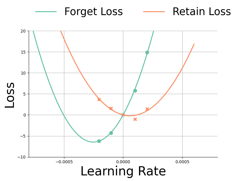
Figure 3: Loss values of retaining and forgetting sets with different learning rates. Markers are $L_{\textup{R}}(\bm{\theta}_{t}-\eta\bm{g}_{\textup{R}})$ and $L_{\textup{F}}(\bm{\theta}_{t}-\eta\bm{g}_{\textup{F}})$ estimated by Phi-1.5 on TOFU at step 10. The curves are fitted as quadratic functions.

4.2 Normalized gradient difference

In order for $L_{\textup{F}}$ to increase as well as $L_{\textup{R}}$ to decrease, we want to construct $\bm{g}_{\text{UN}}$ such that

$$\bm{g}_{\textup{R}}^{\top}\bm{g}_{\text{UN}}(c_{t})\geq 0\geq\bm{g}_{\textup{F}}^{\top}\bm{g}_{\text{UN}}(c_{t}).$$ (7)

To satisfy Eq. (7) , we propose a normalized gradient difference method (NGDiff) to dynamically set $c_{t}=\frac{1/\|\bm{g}_{\textup{R}}\|}{1/\|\bm{g}_{\textup{R}}\|+1/\|\bm{g}_{\textup{F}}\|}\Longrightarrow\bm{g}_{\textup{NGDiff}}(\bm{g}_{\textup{R}},\bm{g}_{\textup{F}}):=\frac{\bm{g}_{\textup{R}}}{\|\bm{g}_{\textup{R}}\|}-\frac{\bm{g}_{\textup{F}}}{\|\bm{g}_{\textup{F}}\|}.$ In words, we normalize the retaining and forgetting gradients

We analyze NGDiff as follows. First, we show the condition in Eq. (7) is satisfied at all iterations in the following lemma (proof in Appendix G):

Lemma 4.

$\bm{g}_{\textup{NGDiff}}(\bm{g}_{\textup{R}},\bm{g}_{\textup{F}})$ satisfies Eq. (7) for any $\bm{g}_{\textup{R}}\in\mathbb{R}^{d}$ and $\bm{g}_{\textup{F}}\in\mathbb{R}^{d}$.

In Theorem 5 (proof in Appendix G), we leverage Lemma 4 to claim that the local loss improvement under appropriate learning rate, which will be implemented adaptively in Section 4.3.

Theorem 5.

Consider $\bm{\theta}_{t+1}=\bm{\theta}_{t}-\eta\bm{g}_{\textup{NGDiff}}$.

(1) Unless $\bm{g}_{\textup{R}}$ is exactly parallel to $\bm{g}_{\textup{F}}$, for any sufficiently small learning rate $\eta$, there exist two constants $\epsilon_{\textup{R},1}=o(\eta),\epsilon_{\textup{F},1}=o(\eta)$ such that

$$\begin{split}L_{\textup{R}}(\bm{\theta}_{t+1})-L_{\textup{R}}(\bm{\theta}_{t})&<\epsilon_{\textup{R},1};\\ L_{\textup{F}}(\bm{\theta}_{t+1})-L_{\textup{F}}(\bm{\theta}_{t})&>\epsilon_{\textup{F},1}.\end{split}$$

(2) If additionally $\bm{g}_{\textup{NGDiff}}^{\top}\mathbf{H}_{\textup{R}}\bm{g}_{\textup{NGDiff}}>0$ and $\bm{g}_{\textup{NGDiff}}^{\top}\mathbf{H}_{\textup{F}}\bm{g}_{\textup{NGDiff}}>0$, then for any learning rate $0<\eta<\frac{2\bm{g}_{\textup{R}}^{\top}\bm{g}_{\textup{NGDiff}}}{\bm{g}_{\textup{NGDiff}}^{\top}\mathbf{H}_{\textup{R}}\bm{g}_{\textup{NGDiff}}}$, there exist two constants $\epsilon_{\textup{R},2}=o(\eta^{2}),\epsilon_{\textup{F},2}=o(\eta^{2})$ such that

$$\begin{split}L_{\textup{R}}(\bm{\theta}_{t+1})-L_{\textup{R}}(\bm{\theta}_{t})&<\epsilon_{\textup{R},2};\\ L_{\textup{F}}(\bm{\theta}_{t+1})-L_{\textup{F}}(\bm{\theta}_{t})&>\epsilon_{\textup{F},2}.\end{split}$$

To interpret Theorem 5, we view $\epsilon\approx 0$ as $\eta$ is generally small (say $\eta\sim 10^{-4}$ in our experiments), and hence, NGDiff is optimizing on R and F simultaneously. Visually speaking, Lemma 4 constrains NGDiff’s gradient to stay in the green area in Figure 2 unless $\bm{g}_{\textup{F}}\parallel\bm{g}_{\textup{R}}$, whereas other methods do not explicitly enforce Eq. (7) and may consequently harm the retaining utility.

We end the analysis with the following remark:

Remark 4.1.

The condition, $\bm{g}_{\textup{NGDiff}}^{\top}\mathbf{H}\bm{g}_{\textup{NGDiff}}>0$ in part (2) of Theorem 5, may not always hold in deep learning. However, it empirically holds in most iterations across models and datasets in our experiments (cf., our Figure 3 and Figure 2 in [4]), and we can stablize the training by not updating $\eta$ when the condition fails.

4.3 Automatic learning rate adaption

In order for NGDiff to work as in Theorem 5, the learning rate schedule needs to be carefully selected so that $0<\eta_{t}<\frac{2\bm{g}_{\textup{R}}^{\top}\bm{g}_{\textup{NGDiff}}}{\bm{g}_{\textup{NGDiff}}^{\top}\mathbf{H}_{\textup{R}}\bm{g}_{\textup{NGDiff}}}$ at each iteration. In Algorithm 1, we adapt GeN [4] (or AutoLR) to the unlearning setting and dynamically set the learning rates as the minimizer of (6): to locally optimize $L_{\textup{R}}$ and to monotonically increase $L_{\textup{F}}$, we use the following learning rate:

$$\eta_{t}^{*}={\bm{g}_{\textup{R}}^{\top}\bm{g}_{\textup{NGDiff}}}/{\bm{g}_{\textup{NGDiff}}^{\top}\mathbf{H}_{\textup{R}}\bm{g}_{\textup{NGDiff}}}.$$ (8)

GeN estimates two scalars – the numerator and denominator of Eq. (8) by analyzing the difference of loss values, thus the high-dimensional Hessian matrix $\mathbf{H}_{\textup{R}}$ is never instantiated. We devote Appendix C to explain how GeN works and how we have modified GeN for unlearning, such as only forward passing on R but not F in Eq. (8).

Remark 4.2.

There is a computational overhead to use GeN, as it requires additional forward passes to estimate $\eta_{t}^{*}$. Nevertheless, we only update the learning rate every 10 iterations so that the overhead is amortized and thus negligible.

Algorithm 1 summarizes NGDiff. We note that $\bm{g}_{\textup{F}},\bm{g}_{\textup{R}}$ can be stochastic gradients.

Algorithm 1 Learning-rate-free NGDiff

1:for $t=1,2,...$ do

2:     —-NGDiff—-

3:     Compute $L_{\textup{R}}(\bm{\theta}_{t})$ by a forward pass on R

4:     Compute $\bm{g}_{\textup{R}}(\bm{\theta}_{t})$ by backward propagation

5:     Compute $L_{\textup{F}}(\bm{\theta}_{t})$ by a forward pass on F

6:     Compute $\bm{g}_{\textup{F}}(\bm{\theta}_{t})$ by backward propagation

7:     Construct $\bm{g}_{\textup{NGDiff}}=\bm{g}_{\textup{R}}/\|\bm{g}_{\textup{R}}\|-\bm{g}_{\textup{F}}/\|\bm{g}_{\textup{F}}\|$

8:     —-AutoLR—-

9:     if $t$ mod $10==0$: then

10:         Compute $L_{R}^{\pm}=L_{\textup{R}}(\bm{\theta}_{t}\pm\eta\bm{g})$ by two forward passes on R

11:         Fit the quadratic function $\mathcal{Q}$ in Eq. (6) from $(-\eta,0,\eta)\to(L_{\textup{R}}^{-},L_{\textup{R}},L_{\textup{R}}^{+})$

12:         Derive the optimal learning rate $\eta_{t}^{*}:=\text{argmin}_{x}\mathcal{Q}(x)$ and set $\eta=\eta_{t}^{*}$      

13:     Update $\theta_{t+1}=\theta_{t}-\eta\bm{g}_{\textup{NGDiff}}$

5 Experiments

5.1 Setup

Dataset We evaluate the empirical performance of our proposed method on the two following datasets (see more dataset details in Section F.1):

Table 1: Performance on TOFU dataset (forget10/retain90) with different unlearning methods and models. We define success as the model being able to reduce Verbatim memorization to below 0.1 or maintain at least 70% of the Model utility and the TruthRatio compared to the No-unlearn, with successful cases highlighted in bold. NGDiff achieves success in most cases.

Base Model	Metric	Method
		No-unlearn	GDiff-0.9	GDiff-0.5	GDiff-0.1	NPO	LossNorm	NGDiff
Phi-1.5	Verbmem $\downarrow$	$1.000$	$0.805$	0.027	0.000	0.000	$0.432$	0.024
	Utility $\uparrow$	$1.000$	$0.992$	$0.308$	$0.000$	$0.000$	0.752	0.747
	TruthRatio $\uparrow$	$0.385$	$0.205$	$0.216$	$0.221$	$0.179$	$0.214$	0.353
Falcon-1B	Verbmem $\downarrow$	$1.000$	0.041	0.001	0.000	0.017	0.055	0.021
	Utility $\uparrow$	$1.000$	0.434	$0.305$	$0.000$	$0.114$	$0.521$	${0.428}$
	TruthRatio $\uparrow$	$0.408$	$0.237$	$0.244$	$0.217$	$0.184$	$0.252$	0.354
GPT2-XL	Verbmem $\downarrow$	$1.000$	0.029	0.001	0.000	0.031	0.022	0.046
	Utility $\uparrow$	$0.999$	$0.381$	$0.250$	$0.000$	$0.136$	$0.376$	0.792
	TruthRatio $\uparrow$	$0.412$	$0.186$	$0.278$	$0.133$	$0.179$	$0.196$	0.399
Llama2-7B	Verbmem $\downarrow$	$1.000$	$0.810$	0.011	0.000	$0.709$	0.010	0.002
	Utility $\uparrow$	$1.000$	0.851	$0.324$	$0.000$	$0.682$	$0.264$	0.724
	TruthRatio $\uparrow$	$0.490$	${0.340}$	0.364	$0.161$	$0.329$	$0.329$	${0.334}$
Mistral-7B	Verbmem $\downarrow$	$1.000$	$1.000$	$0.945$	$0.410$	$0.385$	$0.259$	0.009
	Utility $\uparrow$	$1.000$	0.999	0.944	$0.517$	$0.341$	0.925	0.996
	TruthRatio $\uparrow$	$0.344$	0.345	0.366	0.374	0.364	0.358	0.379

Task of Fictitious Unlearning (TOFU) [36]. TOFU consists of 20 question-answer pairs based on fictitious author biographies generated by GPT-4 [1]. In our experiments, we use the forget10 (10% of the full training set) as the forgetting set and retain90 (90% of the full training set) as the retaining set.

MUSE-NEWS [43]. This dataset consists of BBC news articles [29] published since August 2023. We use its train split to finetune a target model, and then the raw set, which includes both the forgetting and retaining data, for the target model unlearning. Finally, the verbmem and knowmem splits are used to evaluate the unlearned model’s performance.

Unlearning methods We compare NGDiff with 4 baselines. The first baseline method is the target model without any unlearning, while the remaining three are popular unlearning methods.

No-unlearn. We fine-tune the base model on the full training data. Subsequent unlearning approaches are then applied on No-unlearn.

Gradient Difference (GDiff) [31]. GDiff (see Sec. 3.2) applies static linear scalarization with $c=0.5$ in MTO. For a thorough comparison, we also include the extended GDiff method, with $c=0.1$ or $c=0.9$.

Loss Normalization (LossNorm). As discussed in Section 3.2, this approach computes and normalizes the forget loss and retain loss separately, with the overall loss being $L_{\textup{R}}/|L_{\textup{R}}|-L_{\textup{F}}/|L_{\textup{F}}|$.

Negative Preference Optimization (NPO) [55]. NPO uses preference optimization [38] with the loss: $L_{\text{NPO},\beta}(\bm{\theta})=$

$$-\frac{2}{\beta}\mathbb{E}_{\textup{F}}\Big{[}\log\sigma\Big{(}-\beta\log\frac{f(S,w)}{f_{\text{No-unlearn}}(S,w)}\Big{)}\Big{]},$$ (9)

where $S$ is randomly sampled from F, $\beta>0$ is the inverse temperature, $f$ is the unlearned model, and $f_{\text{No-unlearn}}$ is the model before unlearning.

Foundation Models

We test multiple LLMs: LLaMA2-7B [46], Phi-1.5 [28], Falcon-1B [40], GPT2-XL [41] and Mistral-7B [24]. They are pre-trained and then fine-tuned on datasets in Section 5.1, with AdamW optimizer and are carefully tuned (Appendix F).

Base Model	Metric	Method
		No-unlearn	GDiff-0.9	GDiff-0.5	GDiff-0.1	NPO	LossNorm	NGDiff
Llama2-7B	Verbmem $\downarrow$	$0.561$	$0.555$	0.043	0.004	0.000	$0.388$	0.036
	Knowmem $\downarrow$	$0.755$	$0.717$	0.287	0.000	0.000	0.514	0.455
	Utility $\uparrow$	$0.646$	0.641	$0.275$	$0.000$	$0.000$	0.506	0.556
Mistral-7B	Verbmem $\downarrow$	$0.578$	$0.177$	0.000	0.000	$0.113$	$0.196$	0.098
	Knowmem $\downarrow$	$0.416$	0.257	0.000	0.000	$0.343$	$0.293$	0.165
	Utility $\uparrow$	$0.411$	0.339	$0.000$	$0.000$	0.316	0.343	0.354

Table 2: Results on the MUSE-NEWS dataset. We boldface the entries where unlearning successfully reduces Verbatim memorization to below 0.1, reduces Knowledge memorization to less than 70% of No-Unlearn, or maintains at least 70% of the Utility compared to No-Unlearn. With the exception of NGDiff, most unlearning approaches exhibit a significant trade-off between forgetting and utility.

5.2 Evaluation Metrics

Following the existing work [43], we evaluate the unlearning performance based on model’s output quality. We expect a good performance should satisfy the following requirements:

No verbatim memorization. After the unlearning, the model should no longer remember any verbatim copies of the texts in the forgetting data. To evaluate this, we prompt the model with the first $k$ tokens in F and compare the model’s continuation outputs with the ground truth continuations. We use ROUGE-L recall scores for this comparison, where a lower score is better for unlearning.

No knowledge memorization. After the unlearning, the model should not only forget verbatim texts, but also the knowledge in the forgetting set. For the MUSE-NEWS dataset, we evaluate knowledge memorization using the Knowmem${}_{\textup{F}}$ split, which consists of generated question-answer pairs based on the forgetting data. Similar to verbatim memorization, we use ROUGE-L recall scores.

Maintained model utility. An effective unlearning method must maintain the model’s performance on the retaining set. We prompt the model with the question from R and compare the generated answer to the ground truth. We use ROUGE-L recall scores for these comparisons. Additionally, we evaluate the model using the Truth Ratio metric. We use the Retain10-perturbed split from TOFU, which consists of five perturbed answers created by modifying the facts in each original answer from R. The Truth Ratio metric computes how likely the model generates a correct answer versus an incorrect one, where a higher value is better.

Method	TOFU (without $\to$ with AutoLR)
	Verbmem $\downarrow$	Utility $\uparrow$	TruthRatio $\uparrow$
No-unlearn	$1.00$	$1.00$	$0.39$
GDiff c=0.9	$0.81\to 0.20$	$0.99\to 0.42$	$0.21\to 0.31$
GDiff c=0.5	$0.03\to 0.00$	$0.31\to 0.03$	$0.22\to 0.30$
GDiff c=0.1	$0.00\to 0.00$	$0.00\to 0.00$	$0.22\to 0.23$
NPO	$0.00\to 0.00$	$0.00\to 0.00$	$0.18\to 0.22$
LossNorm	$0.43\to 0.23$	$0.75\to 0.73$	$0.21\to 0.34$
NGDiff	$0.02\to 0.01$	$0.61\to 0.75$	$0.29\to 0.35$

Table 3: Influence of AutoLR with different unlearning methods on the Phi-1.5 model. AutoLR improves the TruthRatio and reduces Verbmem across all methods. W/ or w/o AutoLR, NGDiff outperforms other baselines.

5.3 Main Results

The results for Verbatim memorization (Verbmem), Model utility (Utility), TruthRatio, and Knowledge memorization (Knowmem) using different unlearning methods are presented in Table 1, 2 as well as 6 in Appendix. We evaluate these metrics using TOFU and MUSE-NEWS across LLMs.

In summary, our NGDiff consistently achieves the superior performance across all models on both datasets. In stark contrast, the baseline unlearning methods (1) either effectively forget R by reducing Verbmem and Knowmem but fail maintain the Utility and TruthRatio, such as GDiff with $c\leq 0.5$, NPO; (2) or cannot unlearn F on Phi-1.5 and Mistral-7B, such as LossNorm and GDiff with $c=0.9$. We highlight that the effectiveness of these unlearning methods are highly model-dependent and dataset-dependent, unlike NGDiff.

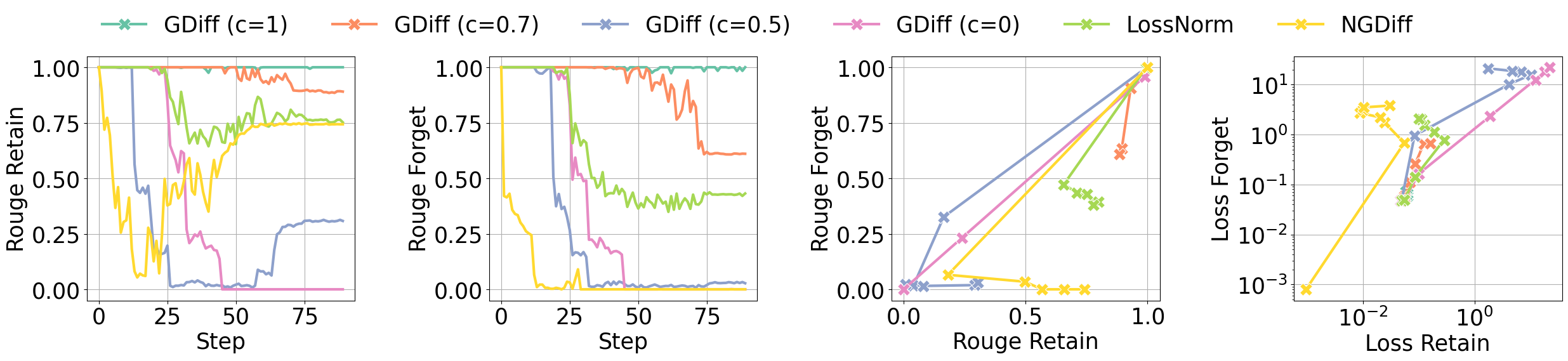
Figure 4: Comparison of unlearning methods on TOFU. The figures show the ROUGE scores and loss terms during unlearning process with different methods, which includes GDiff, LossNorm, and NGDiff. We observe that NGDiff effectively unlearns the forgetting data while maintaining the performance on the retaining data.

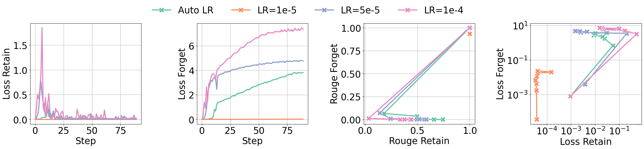
Figure 5: Comparison between AutoLR and different learning rates on NGDiff. The figures show the ROUGE scores and loss values during the unlearning process on TOFU dataset using Phi-1.5 model. We observe that AutoLR outperforms the static learning rates with better model utility and more stable convergence.

For the TOFU dataset, we observe that some unlearning methods fail to unlearn the forget data effectively. For example, GDiff-0.9 and LossNorm do not unlearn effectively when applied to Phi-1.5, Llama2-7B and Mistral-7B. In fact, GDiff-0.9 has $80\%\sim 100\%$ Verbmem and LossNorm has $>40\%$ Verbmem on Phi-1.5. However, they are effective on Falcon-1B and GPT2-XL, even though these models have similar sizes ($\approx 1$B parameters) to Phi-1.5. On the other hand, some methods fail to preserve the model utility after unlearning. For example, GDiff-0.1 has close to 0 Utility on Phi-1.5, Falcon-1B, GPT2-XL and Llama2-7B; similarly, NPO also experiences a significant drop in Utility on Phi-1.5 model, Falcon-1B and GPT2-XL, but not so on Llama2-7B. In contrast, our NGDiff remains effective in unlearning F and maintaining R across the models. In addition, NGDiff achieves the best TruthRatio on all models except Llama2-7B (which is still on par with the best), indicating that the model’s answers remain factually accurate for questions in the retaining data.

For the MUSE-NEWS dataset, NGDiff also outperforms the baseline methods on Llama2-7B and Mistral-7B models by achieving a lower Verbmem and a higher Utility. The Knowmem results indicate that NGDiff not only unlearns the verbatim copies of the forgetting texts, but also successfully removes the associated knowledge. While the model capacities of Phi-1.5 and Falcon-1B are smaller, limiting their ability to learn knowledge effectively after fine-tuning on the full dataset, as shown in Table 6, NGDiff still performs well.

To further illustrate the performance of our proposed method during the training, in addition to the last iterate results, we plot the ROUGE scores and loss terms during the unlearning process in Figure 4. We apply the extended GDiff, LossNorm, and NGDiff methods, to the Phi-1.5 model using the TOFU dataset. While GDiff with $c=0.5$ and $c=0.7$, and NGDiff are effective in unlearning, only NGDiff preserve the model utility above $75\%$ ROUGE score. A closer look at the second and the fourth plots of Figure 4 shows that NGDiff exhibits the fastest and most stable convergence on F while maintaining a low retaining loss $\leq 0.1$.

5.4 Ablation Study

Effectiveness of NGDiff. In our experiments, we utilize the automatic learning rate scheduler (AutoLR) for NGDiff method. To investigate the impact of NGDiff alone, we compare all methods with or without AutoLR in Table 3. With AutoLR or not (where we use manually tuned learning rates), NGDiff, GDiff ($c=0.1$ or $0.5$) and NPO can effectively unlearn in terms of Verbmem. However, among these four methods, NGDiff uniquely retains a reasonable Utility between $60\sim 75\%$, while other methods retains only $0\sim 30\%$ Utility. A similar pattern is observed in terms of TruthRatio as well. Overall, NGDiff significantly outperforms other baseline methods with or without AutoLR.

Impact of automatic learning rate. To evaluate the impact of AutoLR scheduler, we see in Table 3 all methods exhibit an increase in the TruthRatio metric and a decrease in Verbmem, though with some loss in the Utility. For instance, LossNorm benefits significantly from AutoLR with $\approx 20\%$ decrease in Verbmem, and NGDiff increases its retaining Utility and TruthRatio by $>22\%$. We specifically demonstrate the impact of AutoLR on NGDiff in Figure 5. Without AutoLR, the model’s performance is highly sensitive to the static learning rates: when $\eta=10^{-5}$, the model fails to unlearn F as indicated by the low loss and high ROUGE score; in contrast, when $\eta=10^{-4}$, there is a significant drop in ROUGE score on the retain data, falling from 100% to around 50%. However, with the AutoLR scheduler, we observe a steady reduction in the Verbmem (with the ROUGE forget close to 0 at convergence) while maintaining high utility (the ROUGE retain is 0.747, which is 19.5% higher than the best results without AutoLR).

6 Conclusion and Discussion

We formulated the machine unlearning problem as a two-task optimization problem and proposed a novel unlearning method NGDiff based on normalized gradient difference and automatic learning rate adaption. By leveraging insights from multi-task optimization, NGDiff empirically improves forgetting quality while maintaining utility. We hope this paper helps establish a connection between LLM unlearning and multi-task optimization, and inspires further advancements in this field.

Limitations

Like other machine learning approaches in NLP, while our goal is to remove the influence of specific documents from LLMs, complete removal cannot always be guaranteed. Therefore, caution should be exercised when applying the proposed unlearning techniques in practical applications as unlearned LLMs can still potentially generate harmful or undesired outputs.

There are several technical alternatives that we did not explore in this paper due to its scope and limited resources. For example, other learning-rate-free methods could potentially be adapted as alternatives to the GeN approach used in this work. Additionally, other multi-task optimization methods could be applied to machine unlearning. However, scaling these approaches to the level of LLMs could be challenging, and are left as future work.

Finally, we mainly examined NGDiff’s effectiveness on LLM unlearning in this paper with two benchmark datasets, TOFU and MUSE. To show its generalizability, we provide an additional example to apply the algorithm to computer vision tasks (see Appendix D). However, it would be desirable to test NGDiff on other modalities beyond NLP and CV applications.

Appendix A Preliminary evidence

In our preliminary experiments, we observe two key issues preventing the standard methods from being practically applied. First, balancing retaining and forgetting losses is difficult. In Figure 1, we observe a trade-off between the performance on R and F, where some methods fail to unlearn F (points in the upper-right corner of the left figure), and some do not maintain utility in R (points in the bottom-left corner of the left figure). The blue dotted line in Figure 1 further illustrates the trade-off in GDiff by sweeping a hyper-parameter $c\in[0,1],$ which is used to balance the losses on the forgetting and retaining data (see Eq. (3)). Picking an appropriate $c$ to balance the two terms is often challenging. Secondly, the optimization methods for unlearning are usually sensitive to the learning rate. As illustrated in Figure 6, even for the same algorithm, various learning rates lead to substantial changes in the ROUGE scores and loss values, making the unlearning methods unstable and difficult to use in practice.

Figure 6: ROUGE scores and loss values during unlearning with vanilla GDiff (equally weighted), under different learning rates to which the unlearning performance is highly sensitive.

Appendix B Comparing NGDiff with GradNorm

Algorithm 2 NGDiff

1:for $t=1,2,...$ do

2:    Compute retaining loss $L_{\textup{R}}(\bm{\theta}_{t})$ by one forward pass

3:    Compute retaining gradient $\bm{g}_{\textup{R}}(\bm{\theta}_{t})=\nabla_{\bm{\theta}}{L_{\textup{R}}}$

4:    Compute forgetting loss $L_{\textup{F}}(\bm{\theta}_{t})$ by one forward pass

5:    Compute forgetting gradient $\bm{g}_{\textup{F}}(\bm{\theta}_{t})=\nabla_{\bm{\theta}}{L_{\textup{F}}}$

6:    Construct unlearning gradient $\bm{g}_{\textup{NGDiff}}=\bm{g}_{\textup{R}}/\|\bm{g}_{\textup{R}}\|-\bm{g}_{\textup{F}}/\|\bm{g}_{\textup{F}}\|$

7:    Update $\bm{\theta}_{t+1}=\bm{\theta}_{t}-\eta\bm{g}_{\textup{NGDiff}}$

Algorithm 3 GradNorm for two-task

1:Initialize the scalaring coefficients $w_{\textup{R}}(\bm{\theta}_{0})=1$ and $w_{\textup{F}}(\bm{\theta}_{0})=1$

2:Pick value for $\alpha>0$ and pick the weights $\bm{\theta}_{\text{LS}}$ (the last shared layer of $\bm{\theta}_{t}$)

3:for $t=1,2,...$ do

4:    Compute retaining loss $L_{\textup{R}}(\bm{\theta}_{t})$ by one forward pass

5:    Compute retaining gradient $\bm{g}_{\textup{R}}(\bm{\theta}_{\text{LS}})=\nabla_{\bm{\theta}_{\text{LS}}}{L_{\textup{R}}}$

6:    Compute forgetting loss $L_{\textup{F}}(\bm{\theta}_{t})$ by one forward pass

7:    Compute forgetting gradient $\bm{g}_{\textup{F}}(\bm{\theta}_{\text{LS}})=\nabla_{\bm{\theta}_{\text{LS}}}{L_{\textup{F}}}$

8:    Compute loss $L(\bm{\theta}_{t})=w_{\textup{R}}(\bm{\theta}_{t})L_{\textup{R}}(\bm{\theta}_{t})+w_{\textup{F}}(\bm{\theta}_{t})L_{\textup{F}}(\bm{\theta}_{t})$

9:    Compute $\bar{\bm{g}}(\bm{\theta}_{\text{LS}})$ by averaging $\bm{g}_{\textup{R}}$ and $\bm{g}_{\textup{F}}$

10:    Compute GradNorm loss

$$L_{GN}(\bm{\theta}_{t})=|\bm{g}_{\textup{R}}-\bar{\bm{g}}\times[r_{\textup{R}}(t)]^{\alpha}|_{1}+|\bm{g}_{\textup{F}}-\bar{\bm{g}}\times[r_{\textup{F}}(t)]^{\alpha}|_{1}$$

11:    Compute GradNorm gradients $\nabla_{w_{\textup{R}}}L_{GN}$ and $\nabla_{w_{\textup{F}}}L_{GN}\in\textup{R}$

12:    Compute the full gradient $\nabla_{\bm{\theta}_{t}}L$

13:    Update $w_{\textup{R}}(\bm{\theta}_{t})\to w_{\textup{R}}(\bm{\theta}_{t+1})$ and $w_{\textup{F}}(\bm{\theta}_{t})\to w_{\textup{F}}(\bm{\theta}_{t+1})$ using $\nabla_{w_{\textup{R}}}L_{GN}$ and $\nabla_{w_{\textup{F}}}L_{GN}$

14:    Update $\bm{\theta}_{t+1}=\bm{\theta}_{t}-\eta\nabla_{\bm{\theta}_{t}}L$

15:    Renormalize $w_{\textup{R}}(\bm{\theta}_{t+1})$ and $w_{\textup{F}}(\bm{\theta}_{t+1})$ so that $w_{\textup{R}}(\bm{\theta}_{t+1})+w_{\textup{F}}(\bm{\theta}_{t+1})=2$

We compare the GradNorm algorithm [11] with our proposed method, NGDiff. We highlight some steps of GradNorm in red to indicate the differences than NGDiff:

• NGDiff sets the scalaring coefficient as $1/\|\bm{g}_{\textup{R}}\|$ and $1/\|\bm{g}_{\textup{F}}\|$, while GradNorm uses gradient descent to learn these coefficients as $w_{\textup{R}}$ and $w_{\textup{F}}$.

• NGDiff is model-agnostic while GradNorm contains specific designs for multi-task architecture. In unlearning, there are 2 data splits (i.e., F and R) and each data split defines one task. Hence all model parameters are shared. However, in the original form of GradNorm, there is 1 data split on which multiple tasks are defined (can be more than 2). Hence the model parameters are partitioned into [shared layers, task 1 specific layers, task 2 specific layers].

• NGDiff computes the full per-task gradients whereas GradNorm only computes the last shared layer’s gradients.

• NGDiff requires 2 back-propagation at each iteration but GradNorm requires 3 (2 for per-task gradients, 1 for $\nabla_{\bm{\theta}}L$), which may translate to more training time for large models.

• GradNorm introduces additional hyperparameters that can be difficult and costly to tune, and may cause instability of training if not properly tuned. These hyperparameters include $\alpha$ and two learning rates to update $w_{\textup{R}}$ and $w_{\textup{F}}$ in Line 13 of Appendix B. In contrast, NGDiff is hyperparameter-free when equipped with GeN (AutoLR).

• NGDiff are theoretically supported by Theorem 5, while the choice of hyperparameters and the use of a heuristic $r_{i}(t)$ by GradNorm may require further justification. Here $r_{i}(t)=\widetilde{L}_{i}(\bm{\theta}_{t})/\mathbb{E}_{\text{task}}[\widetilde{L}_{i}(\bm{\theta}_{t})]$ is the "relative inverse training rate" of task $i$, where $\widetilde{L}_{i}(\bm{\theta}_{t})=L_{i}(\bm{\theta}_{t})/L_{i}(\bm{\theta}_{0})$, $i\in\{\textup{F},\textup{R}\}$.

In summary, NGDiff is remarkably simpler and more well-suited than GradNorm for unlearning, with stable performance and theoretical ground.

Appendix C Details related to GeN

C.1 Brief introduction of GeN

GeN [4] is a method that sets the learning rate for any given gradient $\bm{d}$ as

$$\eta_{\text{GeN}}=\frac{\mathbf{G}^{\top}\bm{d}}{\bm{d}^{\top}\mathbf{H}\bm{d}}$$

where $\mathbf{G}$ is the gradient and $\mathbf{H}$ is the Hessian matrix of some loss $L$. One only needs to access the scalars $\mathbf{G}^{\top}\bm{d}$ and $\bm{d}^{\top}\mathbf{H}\bm{d}$, without computing the high-dimensional $\mathbf{G}$ and $\mathbf{H}$ (or Hessian-vector product). To do so, two additional forward passes are needed: given a constant (say $\xi=0.001$), we compute $L(\bm{\theta}+\xi\bm{d})$ and $L(\bm{\theta}-\xi\bm{d})$. Then by curve fitting or finite difference as demonstrated below, we can estimate up to arbitrary precision controlled by $\xi$:

$$\mathbf{G}^{\top}\bm{d}\approx\frac{L(\bm{\theta}+\xi\bm{d})-L(\bm{\theta}-\xi\bm{d})}{2\xi}$$

and

$$\bm{d}^{\top}\mathbf{H}\bm{d}\approx\frac{L(\bm{\theta}+\xi\bm{d})-2L(\bm{\theta})+L(\bm{\theta}-\xi\bm{d})}{\xi^{2}}$$

Notice that the regular optimization requires 1 forward pass and 1 back-propagation; GeN requires in total 3 forward passes and 1 back-propagation. Given that back-propagation costs roughly twice the computation time than forward pass, the total time increases from 3 units of time to 5 units. Nevertheless, GeN needs not to be applied at each iteration: if we update the learning rate every 10 iterations as in Remark 4.2, the total time reduces to $3+2/10=3.2$ units, and the overhead is less than 10% compared to the regular optimization.

C.2 Adapting GeN to unlearning

Naively applying GeN to the unlearning will result in

$$\eta_{\text{GeN}}=\frac{\mathbf{G}^{\top}\bm{g}_{\text{UN}}}{\bm{g}_{\text{UN}}^{\top}\mathbf{H}\bm{g}_{\text{UN}}}$$

which minimizes the loss over all datapoints, in both F and R. This is against our goal to maximize the forgetting loss. We must consider the learning rate separately for F and R, as shown in Appendix G (Proof of Theorem 5). When both losses have a convex curvature in Figure 3, the optimal learning rate is only well-defined for $L_{\textup{R}}$ and we do not claim to maximize $L_{\textup{F}}$. In other words, if we minimize $L_{\textup{R}}$, we get to worsen $L_{\textup{F}}$ (though not maximally); if we choose to maximize $L_{\textup{F}}$, we will use infinite learning rate that also maximizes $L_{\textup{R}}$. Therefore, our learning rate in (8) only uses R instead of the whole dataset.

Appendix D Computer Vision Experiments

Method	CIFAR-10		CIFAR-100
	Forget Acc $\downarrow$	Retain Acc $\uparrow$	Forget Acc $\downarrow$	Retain Acc $\uparrow$
No-unlearn	$0.926$	$0.956$	$0.745$	$0.750$
GDiff c=0.9	$0.000$	$0.817$	$0.000$	$0.664$
GDiff c=0.5	$0.000$	$0.830$	$0.000$	$0.609$
GDiff c=0.1	$0.000$	$0.825$	$0.000$	$0.667$
LossNorm	$0.000$	$0.753$	$0.000$	$0.432$
NGDiff	$0.000$	0.931	$0.000$	0.701

Table 4: Results of Forget Acc and Retain Acc using different unlearning methods on the CIFAR-10 dataset. Compared to other baseline methods, NGDiff has the best performance on the model utility.

To demonstrate the effectiveness of unlearning across other modalities, we also evaluate our method on the image classification task. Specifically, we choose the CIFAR-10 and CIFAR-100 dataset [26] and train a ResNet-50 [20] model from scratch. For the CIFAR-10 dataset, we sample 500 images from the class $dog$ as the forgetting data, and use images from the remaining 9 classes as the retaining data. For the CIFAR-100 dataset, we sample 500 images from the class $bed$ as the forgetting data, and use images from the remaining 99 classes as the retaining data. After training, the initial forget data accuracy is $0.926$, and the retain data accuracy is $0.956$ on the CIFAR-10 dataset. The initial forget data accuracy is $0.745$, and the retain data accuracy is $0.750$ on the CIFAR-100 dataset. Then we apply different unlearning methods to the trained models. As shown in Table 4, all methods successfully reduce the forget accuracy to $0$. However, the retaining accuracy of NGDiff remains the highest, which shows its effectiveness in preserving the model utility in image classification tasks.

Appendix E Other Related Works

Machine unlearning

Machine unlearning is oftentimes viewed as a continual learning approach, that removes specific data points after a model has been trained to memorize them. Such removal is light-weighted in contrast to re-training, especially when the forgetting set is much smaller than the retaining. In addition to the methods already introduced in Section 3.2 (namely GA, GDiff and NPO), other methods include SISA [2], influence functions [47], differential privacy [18] and so on. However, these methods could be difficult to scale on large models and large datasets due to the algorithmic complexity. To our best knowledge, this is the first work that formulate the unlearning problem as a two-task problem, which can be solved by a number of well-known MTO methods.

Multi-task optimization

MTO is a paradigm where one model is trained to perform multiple tasks simultaneously, so as to significantly improve the efficiency in contrast to training multiple models, one for each task. The key challenge of MTO is the performance trade-off among tasks, where the multi-task model is worse than single-task model if trained on each task separately. Therefore, the core idea is to balance different tasks by modifying the per-task gradients, e.g. with normalization (LossNorm and NGDiff), PCGrad [52], RLW [30], IMTL [33], MGDA [16], CAGrad [32], GradVaccine [49], GradDrop [12], RotoGrad [23], etc.

Learning-rate-free methods

Parameter-free or learning-rate-free methods automatically set the learning rate scheduler without the hyperparameter tuning, which is computationally infeasible for LLMs, e.g. LLAMA2 pre-training uses 3 hyperparameters just for the learning rate: warmup steps, peak learning rate, and minimum learning rate. At high level, there are two approaches to learning-rate-free methods.

On one hand, GeN [4] leverages the Taylor expansion and convex-like landscape of deep learning, which is applicable for the general purpose, even if the gradient is modified like in the unlearning.

On the other hand, methods like D-adaptation [14], Prodigy [37], DoG [21], DoWG [25] are based on the convex and $G$-Lipschitz conditions: $L(\bar{\theta}_{T})-L(\bm{\theta}_{*})\leq\frac{|\theta_{0}-\theta_{*}|^{2}}{2\eta T}+\frac{\eta G^{2}}{2}$ where $\theta_{*}$ is the unknown minimizer of $L$ and $\bar{\theta}_{T}$ is an averaging scheme of $\{\theta_{0},...,\theta_{T}\}$. With the same theoretical foundation, these methods propose different ways to approximate the initial-to-final distance $|\theta_{0}-\theta_{*}|$. There are two main issues to apply these methods on the unlearning. Firstly, the assumption of $G$-Lipschitz is hard to verify and the minimizer $\theta_{*}$ is not well-defined in multi-objective (see our discussion on Pareto optimality under Lemma 2). Secondly, the optimal learning rate $\frac{|\theta_{0}-\theta_{*}|}{G\sqrt{T}}$ is defined in a manner to minimize the loss, whereas MTO methods operate on the gradient level. Hence MTO is incompatible to such parameter-free methods given that we cannot derive a corresponding loss (e.g. there exists no $L_{\textup{NGDiff}}$ such that $\frac{\partial L_{\textup{NGDiff}}}{\partial\theta}=\bm{g}_{\textup{NGDiff}}$).

Appendix F Experiments

F.1 Datasets

Dataset	TOFU			MUSE-NEWS
	Full	Forget10	Retain90	Train	Raw	VerbmemF	KnowmemF	KnowmemR
# samples	$4,000$	$400$	$3,600$	$7,110$	$2,669$	$100$	$100$	$100$

Table 5: Statistics of the TOFU and MUSE-NEWS datasets. For the TOFU dataset, we use Full split for training the target model, Forget10 and Retain90 as the forgetting and retaining split for unlearning experiments. For the MUSE-NEWS dataset, we utilize Train split for training, Raw split for unlearning. For evaluation, we use Verbmem_F and Knowmem_F splits from forgetting data, and Knowmem_R split from the retaining data.

To evaluate the empirical performance of our proposed method, we experiment on the following datasets in Table 5.

• Task of Fictitious Unlearning (TOFU) [36]. This dataset consists of question-answer pairs based on fictitious author biographies generated by GPT-4 [1]. Initially, predefined attributes, such as birthplace, gender, and writing genre, are assigned to 200 distinct authors. GPT-4 is then prompted to generate detailed information about each author. Following the synthesized data, 20 question-answer pairs are created for each fictitious author. The dataset is then divided into distinct datasets: the retaining set and the forgetting set. In our experiments, we use the forget10 and retain90 split, which excludes 10% of the original dataset.

• MUSE-NEWS [43]. This dataset consists of BBC news articles [29] from August 2023. It includes seven subsets of news data: raw, verbmem, knowmem, privleak, scal, sust, and train. We utilize the train split to finetune a target model, and then the raw set, which includes both the forget and retain data, for the target model unlearning. Then, we use verbmem, knowmem split to evaluate the unlearned model’s performance.

F.2 Evaluation Metrics

Following the existing work [43], we evaluate the unlearning performance based on the quality of outputs from the model after unlearning. We expect a good performance should satisfy the following requirements:

No verbatim memorization We evaluate this metric by prompting the model with the first $l$ tokens of the news data in the forget set and compare the model’s continuation outputs with the ground truth continuation. Specifically, for each input $x\in F$, we choose $x_{[:l]}$ as input, and compare the output $f(x_{[:l]})$ with the ground truth continuation $x_{[l+1:]}$ with the ROUGE-L recall score:

$$\begin{split}&\textit{Verbmem}(f,F)\\ &=\frac{1}{\|F\|}\Sigma_{x}\>\textsc{ROUGE-L}(f(x_{[:l]}),x_{[l+1:]})\end{split}$$ (10)

No knowledge memorization To evaluate this metric, we use the generated question-answer pair based on each example $x\in F$. We prompt the model with the question part $q$ and compare the output answer $f(q)$ to the ground truth answer $a$ using ROUGE-L recall scores:

$$\textit{Knowmem}(f,F)=\frac{1}{\|F\|}\Sigma_{x}\>\textsc{ROUGE-L}(f(q),a)$$ (11)

Maintained model utility An effective unlearning method should also maintain the model’s performance on the retain data. For the MUSE-NEWS dataset, we use the Knowmem_r split, which consists of the generated question-answer pairs based on the retain data. For the TOFU dataset, we prompt the model with the question from the retain set and compare the generated answer with the ground truth. We use ROUGE-L recall scores for evaluation:

$$\textit{Utility}(f,R)=\frac{1}{\|R\|}\Sigma_{x}\>\textsc{ROUGE-L}(f(q),a)$$ (12)

Additionally, we evaluate the model using the Retain10-perturbed split from the TOFU dataset. It consists of five perturbed answers for each original answer, keeping original template but modifying the facts. We compute the Truth Ratio metric, which compares the likelihood of the model generating a correct answer versus an incorrect one for each question in the retain set. A higher Truth Ratio indicates better model utility that effectively remembers knowledge from the retain data.

F.3 Hyper-parameter Settings

To finetune a targeted model with the full dataset, we use the optimizer Adam with a learning rate of $\eta=\{10^{-5},2*10^{-5}\}$, a training batch size of {16, 32}, and train 25 epochs for all language models. For the unlearning process, we use the optimizer Adam with a learning rate $\eta=\{10^{-5},5*10^{-5},10^{-4}\}$, and train 15 epochs for all unlearning methods.

F.4 Other unlearning results

Base Model	Metric	Method
		No-unlearn	GDiff-0.9	GDiff-0.5	GDiff-0.1	NPO	LossNorm	NGDiff
Phi-1.5	Verbmem $\downarrow$	$0.018$	$0.000$	$0.012$	$0.000$	$0.000$	$0.012$	0.004
	Utility $\uparrow$	$0.372$	$0.277$	$0.061$	$0.000$	$0.000$	$0.061$	0.001
	Knowmem $\downarrow$	$0.030$	$0.000$	$0.002$	$0.000$	$0.000$	$0.002$	0.023
Falcon-1B	Verbmem $\downarrow$	$0.204$	$0.132$	$0.000$	$0.000$	$0.000$	$0.126$	0.000
	Utility $\uparrow$	$0.386$	$0.214$	$0.000$	$0.000$	$0.000$	$0.142$	0.025
	Knowmem $\downarrow$	$0.232$	$0.078$	$0.000$	$0.000$	$0.000$	$0.130$	0.087

Table 6: Results of Verbatim memorization, Model utility, and TruthRatio on MUSE-NEWS dataset with different unlearning methods on Phi-1.5, and Falcon-1B models. Lower Verbmem along with higher Utility and TruthRatio indicate a more superior unlearning strategy.

More results on MUSE-NEWS dataset with Phi-1.5 model and Falcon-1B model are in Table 6.

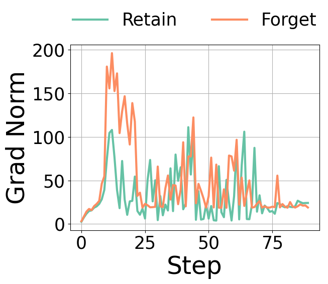
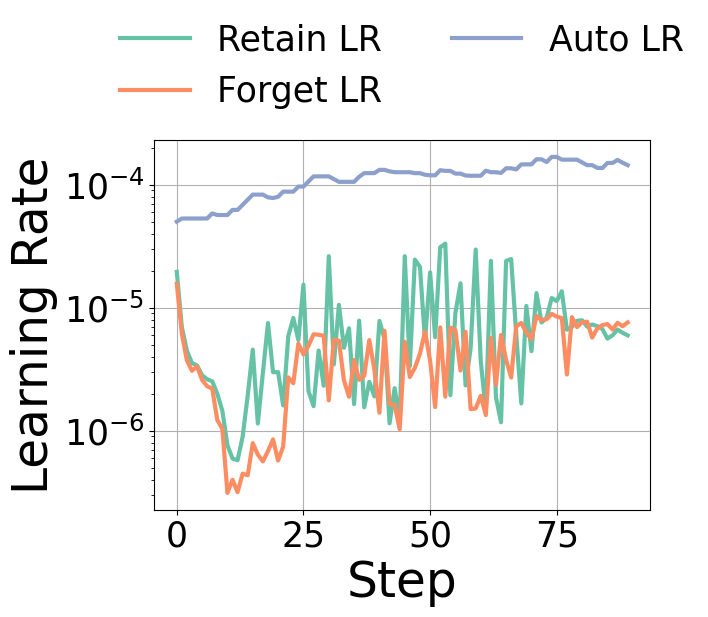
Figure 7: Gradient norms and learning rates during the unlearning on TOFU dataset using NGDiff and Phi-1.5 model. The AutoLR scheduler assigns a smaller learning rate to the forgetting gradient, effectively preserving model utility on the retaining set.

F.5 Visualization of learning rate scheduling

We monitor the gradient norms and the learning rate in Figure 7 for Algorithm 1. We observe that the automatic learning rate is indeed effective, picking up from $5e-5$ to around $2e-4$, and that NGDiff assigns a smaller learning rate to the forgetting gradient, not perturbing the model too much to maintain the high utility on the retaining set.

Appendix G Proofs

In this section, we provide the proofs of all the lemma and theorems in this paper.

Lemma 2 (restated from [51]).

For any $0<c<1$, the model $\bm{\theta}^{*}_{\text{LSP}}(c)=\text{argmin}_{\theta}\textup{LSP}(\bm{\theta};c)$ is Pareto optimal.

Proof of Lemma 2.

We show that the solution of LSP cannot be a dominated point, and therefore it must be Pareto optimal. Consider a solution $\bm{\theta}^{*}=\text{argmin}_{\theta}\textup{LSP}(\bm{\theta};c)$, and suppose it is dominated by some $\bm{\theta}^{\prime}$, i.e. $L_{\textup{F}}(\bm{\theta}^{*})\leq L_{\textup{F}}(\bm{\theta}^{\prime}),L_{\textup{R}}(\bm{\theta}^{*})\geq L_{\textup{R}}(\bm{\theta}^{\prime})$ with at least one inequality being strict. This contradicts that $\bm{\theta}^{*}$ is minimal as $cL_{\textup{R}}(\bm{\theta}^{*})-(1-c)L_{\textup{F}}(\bm{\theta}^{*})>cL_{\textup{R}}(\bm{\theta}^{\prime})-(1-c)L_{\textup{F}}(\bm{\theta}^{\prime}).$ ∎

Theorem 3.

For any $\{c_{t}\}$ with $0\leq c_{t}\leq 1$ that converges as $t\to\infty$, the model $\bm{\theta}^{*}(\{c_{t}\})=\lim_{t\to\infty}\bm{\theta}_{t}$ in (5) is Pareto optimal.

Proof of Theorem 3.

Let $c=\lim_{t}c_{t}$, then Eq. (5) gives that $\bm{g}_{\text{UN}}(\bm{\theta}_{t})=c_{t}\bm{g}_{\textup{R}}(\bm{\theta}_{t})-(1-c_{t})\bm{g}_{\textup{F}}(\bm{\theta}_{t})\to c\bm{g}_{\textup{R}}(\bm{\theta}^{*})-(1-c)\bm{g}_{\textup{F}}(\bm{\theta}^{*})=\bm{0}$ as $t\to\infty$. Note $\bm{\theta}^{*}(\{c_{t}\})$ is equivalent to the LSP solution $\bm{\theta}^{*}_{\text{LSP}}(c)=\text{argmin}_{\theta}\textup{LSP}(\bm{\theta};c)$ as the latter has the same stationary condition, which is Pareto optimal by Lemma 2. ∎

Lemma 4.

$\bm{g}_{\textup{NGDiff}}(\bm{g}_{\textup{R}},\bm{g}_{\textup{F}})$ satisfies Eq. (7) for any $\bm{g}_{\textup{R}}\in\mathbb{R}^{d}$ and $\bm{g}_{\textup{F}}\in\mathbb{R}^{d}$.

Proof of Lemma 4.

We firstly show $\bm{g}_{\textup{R}}^{\top}\bm{g}_{\text{UN}}\geq 0$ for $\bm{g}_{\text{UN}}=\bm{g}_{\textup{NGDiff}}$. We write

$$\begin{split}\bm{g}_{\textup{R}}^{\top}\bm{g}_{\textup{NGDiff}}&=\bm{g}_{\textup{R}}^{\top}\left(\frac{\bm{g}_{\textup{R}}}{\|\bm{g}_{\textup{R}}\|}-\frac{\bm{g}_{\textup{F}}}{\|\bm{g}_{\textup{F}}\|}\right)\\ &=\|\bm{g}_{\textup{R}}\|-\frac{\bm{g}_{\textup{R}}^{\top}\bm{g}_{\textup{F}}}{\|\bm{g}_{\textup{F}}\|}\geq\|\bm{g}_{\textup{R}}\|-\frac{\|\bm{g}_{\textup{R}}\|\|\bm{g}_{\textup{F}}\|}{\|\bm{g}_{\textup{F}}\|}\\ &=0\end{split}$$

where the inequality is the Cauchy-Schwarz inequality. Similarly, $\bm{g}_{\textup{F}}^{\top}\bm{g}_{\text{UN}}\leq 0$ easily follows. ∎

Theorem 5.

Consider $\bm{\theta}_{t+1}=\bm{\theta}_{t}-\eta\bm{g}_{\textup{NGDiff}}$.

(1) Unless $\bm{g}_{\textup{R}}$ is exactly parallel to $\bm{g}_{\textup{F}}$, for any sufficiently small learning rate $\eta$, there exist two constants $\epsilon_{\textup{R},1}=o(\eta),\epsilon_{\textup{F},1}=o(\eta)$ such that

$$L_{\textup{R}}(\bm{\theta}_{t+1})-L_{\textup{R}}(\bm{\theta}_{t})<\epsilon_{\textup{R},1};$$

$$L_{\textup{F}}(\bm{\theta}_{t+1})-L_{\textup{F}}(\bm{\theta}_{t})>\epsilon_{\textup{F},1}.$$

(2) If additionally $\bm{g}_{\textup{NGDiff}}^{\top}\mathbf{H}_{\textup{R}}\bm{g}_{\textup{NGDiff}}>0$ and $\bm{g}_{\textup{NGDiff}}^{\top}\mathbf{H}_{\textup{F}}\bm{g}_{\textup{NGDiff}}>0$, then for any learning rate $0<\eta<\frac{2\bm{g}_{\textup{R}}^{\top}\bm{g}_{\textup{NGDiff}}}{\bm{g}_{\textup{NGDiff}}^{\top}\mathbf{H}_{\textup{R}}\bm{g}_{\textup{NGDiff}}}$, there exist two constants $\epsilon_{\textup{R},2}=o(\eta^{2}),\epsilon_{\textup{F},2}=o(\eta^{2})$ such that

$$L_{\textup{R}}(\bm{\theta}_{t+1})-L_{\textup{R}}(\bm{\theta}_{t})<\epsilon_{\textup{R},2};L_{\textup{F}}(\bm{\theta}_{t+1})-L_{\textup{F}}(\bm{\theta}_{t})>\epsilon_{\textup{F},2}.$$

Proof of Theorem 5.

Applying (6) with $\bm{g}_{\textup{NGDiff}}$ gives

$$L_{\textup{R}}(\bm{\theta}_{t+1})-L_{\textup{R}}(\bm{\theta}_{t})=-\eta\bm{g}_{\textup{R}}^{\top}\bm{g}_{\textup{NGDiff}}+\frac{\eta^{2}}{2}\bm{g}_{\textup{NGDiff}}^{\top}\mathbf{H}_{\textup{R}}\bm{g}_{\textup{NGDiff}}+o(\eta^{2})$$ (13)

For part (1), note that Lemma 4 gives $\bm{g}_{\textup{R}}^{\top}\bm{g}_{\text{NGDiff}}>0$ unless $\bm{g}_{\textup{F}}\parallel\bm{g}_{\textup{R}}$. Hence for any $\eta>0$, we have

$$L_{\textup{R}}(\bm{\theta}_{t+1})-L_{\textup{R}}(\bm{\theta}_{t})=-\eta\bm{g}_{\textup{R}}^{\top}\bm{g}_{\textup{NGDiff}}+o(\eta)<o(\eta)$$

and similarly for $L_{\textup{F}}$.

For part (2), now that $\bm{g}_{\textup{NGDiff}}^{\top}\mathbf{H}_{\textup{R}}\bm{g}_{\textup{NGDiff}}>0$, we have

$$\begin{split}&-\eta\bm{g}_{\textup{R}}^{\top}\bm{g}_{\textup{NGDiff}}+\frac{\eta^{2}}{2}\bm{g}_{\textup{NGDiff}}^{\top}\mathbf{H}_{\textup{R}}\bm{g}_{\textup{NGDiff}}<0\Longleftrightarrow 0<\eta<\frac{2\bm{g}_{\textup{R}}^{\top}\bm{g}_{\textup{NGDiff}}}{\bm{g}_{\textup{NGDiff}}^{\top}\mathbf{H}_{\textup{R}}\bm{g}_{\textup{NGDiff}}}\end{split}$$

and similarly

$$-\eta\bm{g}_{\textup{F}}^{\top}\bm{g}_{\textup{NGDiff}}+\frac{\eta^{2}}{2}\bm{g}_{\textup{NGDiff}}^{\top}\mathbf{H}_{\textup{F}}\bm{g}_{\textup{NGDiff}}>0\Longleftarrow 0<\eta$$

We complete the proof by substituting the inequalities into (13). ∎

References

- [1] Josh Achiam, Steven Adler, Sandhini Agarwal, Lama Ahmad, Ilge Akkaya, Florencia Leoni Aleman, Diogo Almeida, Janko Altenschmidt, Sam Altman, Shyamal Anadkat, et al. Gpt-4 technical report. arXiv preprint arXiv:2303.08774, 2023.
- [2] Lucas Bourtoule, Varun Chandrasekaran, Christopher A Choquette-Choo, Hengrui Jia, Adelin Travers, Baiwu Zhang, David Lie, and Nicolas Papernot. Machine unlearning. In 2021 IEEE Symposium on Security and Privacy (SP), pages 141–159. IEEE, 2021.
- [3] Stephen Boyd and Lieven Vandenberghe. Convex optimization. Cambridge university press, 2004.
- [4] Zhiqi Bu and Shiyun Xu. Automatic gradient descent with generalized newton’s method. arXiv preprint arXiv:2407.02772, 2024.
- [5] Nicholas Carlini, Florian Tramer, Eric Wallace, Matthew Jagielski, Ariel Herbert-Voss, Katherine Lee, Adam Roberts, Tom Brown, Dawn Song, Ulfar Erlingsson, et al. Extracting training data from large language models. In 30th USENIX Security Symposium (USENIX Security 21), pages 2633–2650, 2021.
- [6] Jiaao Chen and Diyi Yang. Unlearn what you want to forget: Efficient unlearning for LLMs. In Houda Bouamor, Juan Pino, and Kalika Bali, editors, Proceedings of the 2023 Conference on Empirical Methods in Natural Language Processing, pages 12041–12052, Singapore, December 2023. Association for Computational Linguistics.
- [7] Kongyang Chen, Zixin Wang, Bing Mi, Waixi Liu, Shaowei Wang, Xiaojun Ren, and Jiaxing Shen. Machine unlearning in large language models. arXiv preprint arXiv:2404.16841, 2024.
- [8] Liang Chen, Shuming Ma, Dongdong Zhang, Furu Wei, and Baobao Chang. On the pareto front of multilingual neural machine translation. ArXiv, abs/2304.03216, 2023.
- [9] Shijie Chen, Yu Zhang, and Qiang Yang. Multi-task learning in natural language processing: An overview. ACM Computing Surveys, 2021.
- [10] Zhao Chen, Vijay Badrinarayanan, Chen-Yu Lee, and Andrew Rabinovich. Gradnorm: Gradient normalization for adaptive loss balancing in deep multitask networks. In International conference on machine learning, pages 794–803. PMLR, 2018.
- [11] Zhao Chen, Vijay Badrinarayanan, Chen-Yu Lee, and Andrew Rabinovich. Gradnorm: Gradient normalization for adaptive loss balancing in deep multitask networks, 2018.
- [12] Zhao Chen, Jiquan Ngiam, Yanping Huang, Thang Luong, Henrik Kretzschmar, Yuning Chai, and Dragomir Anguelov. Just pick a sign: Optimizing deep multitask models with gradient sign dropout, 2020.
- [13] Nicola De Cao, Wilker Aziz, and Ivan Titov. Editing factual knowledge in language models. In Marie-Francine Moens, Xuanjing Huang, Lucia Specia, and Scott Wen-tau Yih, editors, Proceedings of the 2021 Conference on Empirical Methods in Natural Language Processing, pages 6491–6506, Online and Punta Cana, Dominican Republic, November 2021. Association for Computational Linguistics.
- [14] Aaron Defazio and Konstantin Mishchenko. Learning-rate-free learning by d-adaptation, 2023.
- [15] A. P. Dempster, N. M. Laird, and D. B. Rubin. Maximum likelihood from incomplete data via the EM algorithm. Journal of the Royal Statistical Society: Series B, 39:1–38, 1977.
- [16] Jean-Antoine Désidéri. Multiple-gradient descent algorithm (mgda) for multiobjective optimization. Comptes Rendus Mathematique, 350(5-6):313–318, 2012.
- [17] Ronen Eldan and Mark Russinovich. Who’s harry potter? approximate unlearning in llms. 2023.
- [18] Varun Gupta, Christopher Jung, Seth Neel, Aaron Roth, Saeed Sharifi-Malvajerdi, and Chris Waites. Adaptive machine unlearning. Advances in Neural Information Processing Systems, 34:16319–16330, 2021.
- [19] Xudong Han, Timothy Baldwin, and Trevor Cohn. Fair enough: Standardizing evaluation and model selection for fairness research in NLP. In Andreas Vlachos and Isabelle Augenstein, editors, Proceedings of the 17th Conference of the European Chapter of the Association for Computational Linguistics, pages 297–312, Dubrovnik, Croatia, May 2023. Association for Computational Linguistics.
- [20] Kaiming He, Xiangyu Zhang, Shaoqing Ren, and Jian Sun. Deep residual learning for image recognition, 2015.
- [21] Maor Ivgi, Oliver Hinder, and Yair Carmon. Dog is sgd’s best friend: A parameter-free dynamic step size schedule, 2023.
- [22] Joel Jang, Dongkeun Yoon, Sohee Yang, Sungmin Cha, Moontae Lee, Lajanugen Logeswaran, and Minjoon Seo. Knowledge unlearning for mitigating privacy risks in language models. In Anna Rogers, Jordan Boyd-Graber, and Naoaki Okazaki, editors, Proceedings of the 61st Annual Meeting of the Association for Computational Linguistics (Volume 1: Long Papers), pages 14389–14408, Toronto, Canada, July 2023. Association for Computational Linguistics.
- [23] Adrián Javaloy and Isabel Valera. Rotograd: Gradient homogenization in multitask learning, 2022.
- [24] Albert Q Jiang, Alexandre Sablayrolles, Arthur Mensch, Chris Bamford, Devendra Singh Chaplot, Diego de las Casas, Florian Bressand, Gianna Lengyel, Guillaume Lample, Lucile Saulnier, et al. Mistral 7b. arXiv preprint arXiv:2310.06825, 2023.
- [25] Ahmed Khaled, Konstantin Mishchenko, and Chi Jin. Dowg unleashed: An efficient universal parameter-free gradient descent method, 2024.
- [26] Alex Krizhevsky, Geoffrey Hinton, et al. Learning multiple layers of features from tiny images. 2009.
- [27] Yige Li, Hanxun Huang, Yunhan Zhao, Xingjun Ma, and Jun Sun. Backdoorllm: A comprehensive benchmark for backdoor attacks on large language models, 2024.
- [28] Yuanzhi Li, Sébastien Bubeck, Ronen Eldan, Allie Del Giorno, Suriya Gunasekar, and Yin Tat Lee. Textbooks are all you need ii: phi-1.5 technical report. arXiv preprint arXiv:2309.05463, 2023.
- [29] Yucheng Li, Frank Geurin, and Chenghua Lin. Avoiding data contamination in language model evaluation: Dynamic test construction with latest materials. arXiv preprint arXiv:2312.12343, 2023.
- [30] Baijiong Lin, Feiyang Ye, Yu Zhang, and Ivor Tsang. Reasonable effectiveness of random weighting: A litmus test for multi-task learning. Transactions on Machine Learning Research, 2021.
- [31] Bo Liu, Qiang Liu, and Peter Stone. Continual learning and private unlearning. In Conference on Lifelong Learning Agents, pages 243–254. PMLR, 2022.
- [32] Bo Liu, Xingchao Liu, Xiaojie Jin, Peter Stone, and Qiang Liu. Conflict-averse gradient descent for multi-task learning, 2024.
- [33] Liyang Liu, Yi Li, Zhanghui Kuang, J Xue, Yimin Chen, Wenming Yang, Qingmin Liao, and Wayne Zhang. Towards impartial multi-task learning. In iclr, 2021.
- [34] Sijia Liu, Yuanshun Yao, Jinghan Jia, Stephen Casper, Nathalie Baracaldo, Peter Hase, Xiaojun Xu, Yuguang Yao, Hang Li, Kush R Varshney, et al. Rethinking machine unlearning for large language models. arXiv preprint arXiv:2402.08787, 2024.
- [35] Sijia Liu, Yuanshun Yao, Jinghan Jia, Stephen Casper, Nathalie Baracaldo, Peter Hase, Yuguang Yao, Chris Yuhao Liu, Xiaojun Xu, Hang Li, Kush R. Varshney, Mohit Bansal, Sanmi Koyejo, and Yang Liu. Rethinking machine unlearning for large language models, 2024.
- [36] Pratyush Maini, Zhili Feng, Avi Schwarzschild, Zachary C Lipton, and J Zico Kolter. Tofu: A task of fictitious unlearning for llms. arXiv preprint arXiv:2401.06121, 2024.
- [37] Konstantin Mishchenko and Aaron Defazio. Prodigy: An expeditiously adaptive parameter-free learner, 2024.
- [38] Long Ouyang, Jeff Wu, Xu Jiang, Diogo Almeida, Carroll L. Wainwright, Pamela Mishkin, Chong Zhang, Sandhini Agarwal, Katarina Slama, Alex Ray, John Schulman, Jacob Hilton, Fraser Kelton, Luke Miller, Maddie Simens, Amanda Askell, Peter Welinder, Paul Christiano, Jan Leike, and Ryan Lowe. Training language models to follow instructions with human feedback, 2022.
- [39] Martin Pawelczyk, Seth Neel, and Himabindu Lakkaraju. In-context unlearning: Language models as few shot unlearners. In ICML, 2024.
- [40] Guilherme Penedo, Quentin Malartic, Daniel Hesslow, Ruxandra Cojocaru, Alessandro Cappelli, Hamza Alobeidli, Baptiste Pannier, Ebtesam Almazrouei, and Julien Launay. The refinedweb dataset for falcon llm: Outperforming curated corpora with web data, and web data only, 2023.
- [41] Alec Radford, Jeffrey Wu, Rewon Child, David Luan, Dario Amodei, Ilya Sutskever, et al. Language models are unsupervised multitask learners. OpenAI blog, 1(8):9, 2019.
- [42] Rajhans Samdani, Ming-Wei Chang, and Dan Roth. Unified expectation maximization. In Eric Fosler-Lussier, Ellen Riloff, and Srinivas Bangalore, editors, Proceedings of the 2012 Conference of the North American Chapter of the Association for Computational Linguistics: Human Language Technologies, pages 688–698, Montréal, Canada, June 2012. Association for Computational Linguistics.
- [43] Weijia Shi, Jaechan Lee, Yangsibo Huang, Sadhika Malladi, Jieyu Zhao, Ari Holtzman, Daogao Liu, Luke Zettlemoyer, Noah A Smith, and Chiyuan Zhang. Muse: Machine unlearning six-way evaluation for language models. arXiv preprint arXiv:2407.06460, 2024.
- [44] Nianwen Si, Hao Zhang, Heyu Chang, Wenlin Zhang, Dan Qu, and Weiqiang Zhang. Knowledge unlearning for llms: Tasks, methods, and challenges, 2023.
- [45] The New York Times. Exhibit j, 2023.
- [46] Hugo Touvron, Louis Martin, Kevin Stone, Peter Albert, Amjad Almahairi, Yasmine Babaei, Nikolay Bashlykov, Soumya Batra, Prajjwal Bhargava, Shruti Bhosale, et al. Llama 2: Open foundation and fine-tuned chat models. arXiv preprint arXiv:2307.09288, 2023.
- [47] Enayat Ullah, Tung Mai, Anup Rao, Ryan A Rossi, and Raman Arora. Machine unlearning via algorithmic stability. In Conference on Learning Theory, pages 4126–4142. PMLR, 2021.
- [48] Eric Wallace, Tony Zhao, Shi Feng, and Sameer Singh. Concealed data poisoning attacks on NLP models. In Kristina Toutanova, Anna Rumshisky, Luke Zettlemoyer, Dilek Hakkani-Tur, Iz Beltagy, Steven Bethard, Ryan Cotterell, Tanmoy Chakraborty, and Yichao Zhou, editors, Proceedings of the 2021 Conference of the North American Chapter of the Association for Computational Linguistics: Human Language Technologies, pages 139–150, Online, June 2021. Association for Computational Linguistics.
- [49] Zirui Wang, Yulia Tsvetkov, Orhan Firat, and Yuan Cao. Gradient vaccine: Investigating and improving multi-task optimization in massively multilingual models, 2020.
- [50] Xiaobao Wu, Liangming Pan, William Yang Wang, and Anh Tuan Luu. Akew: Assessing knowledge editing in the wild, 2024.
- [51] Derrick Xin, Behrooz Ghorbani, Justin Gilmer, Ankush Garg, and Orhan Firat. Do current multi-task optimization methods in deep learning even help? Advances in neural information processing systems, 35:13597–13609, 2022.
- [52] Tianhe Yu, Saurabh Kumar, Abhishek Gupta, Sergey Levine, Karol Hausman, and Chelsea Finn. Gradient surgery for multi-task learning. Advances in Neural Information Processing Systems, 33:5824–5836, 2020.
- [53] Alan L Yuille and Anand Rangarajan. The concave-convex procedure (cccp). In T. Dietterich, S. Becker, and Z. Ghahramani, editors, Advances in Neural Information Processing Systems, volume 14. MIT Press, 2001.
- [54] Dawen Zhang, Pamela Finckenberg-Broman, Thong Hoang, Shidong Pan, Zhenchang Xing, Mark Staples, and Xiwei Xu. Right to be forgotten in the era of large language models: Implications, challenges, and solutions, 2024.
- [55] Ruiqi Zhang, Licong Lin, Yu Bai, and Song Mei. Negative preference optimization: From catastrophic collapse to effective unlearning. arXiv preprint arXiv:2404.05868, 2024.
- [56] Zhihan Zhang, Wenhao Yu, Mengxia Yu, Zhichun Guo, and Meng Jiang. A survey of multi-task learning in natural language processing: Regarding task relatedness and training methods. In Andreas Vlachos and Isabelle Augenstein, editors, Proceedings of the 17th Conference of the European Chapter of the Association for Computational Linguistics, pages 943–956, Dubrovnik, Croatia, May 2023. Association for Computational Linguistics.