Joint Estimation of Conditional Mean and Covariance for Unbalanced Panels333We thank Sam Cohen, Olivier Scaillet, Raman Uppal, Michael Wolf, and participants of the Oxford Man Institute Machine Learning in Quantitative Finance Conference 2024, the 17th International Conference on Computational and Financial Econometrics (CFE 2023), the York Asset Pricing Workshop (2024), and seminars at the Universities of St. Gallen, Geneva, Lugano, Cambridge, and Zürich for helpful comments. Paul Schneider is gratefully acknowledges the Swiss National Science Foundation grant 105218_215528 “Large-scale kernel methods in financial economics”.
Damir Filipović111EPFL and SFI,
damir.filipovic@epfl.chPaul Schneider222Università della Svizzera italiana and SFI,
paul.schneider@usi.ch
(28 October 2024)
Abstract
We propose a novel nonparametric kernel-based estimator of cross-sectional conditional mean and covariance matrices for large unbalanced panels. We show its consistency and provide finite-sample guarantees. In an empirical application, we estimate conditional mean and covariance matrices for a large unbalanced panel of monthly stock excess returns given macroeconomic and firm-specific covariates from 1962 to 2021.
The estimator performs well with respect to statistical measures. It is informative for empirical asset pricing, generating conditional mean-variance efficient portfolios with substantial out-of-sample Sharpe ratios far beyond equal-weighted benchmarks.
1 Introduction
The relation between expected returns and conditional risk of assets and their characteristics is a long investigated topic in financial economics. To this date, statistical inference is severely hindered by the unbalanced and high-dimensional nature of the data, however. In this paper, we propose a resolution of the econometric conditional inference problem by means of a highly tractable nonparametric framework in which conditional moments are functions of characteristics, resolving a long-standing and important challenge in cross-sectional asset pricing posited in Cochrane (2011). Our proposal is constructed precisely such that it maintains symmetric and positive semidefinite covariance matrices in all states of the world, and for cross sections of any size.
Starting from Fama and
MacBeth (1973), the tools available to the empirical researcher in the context of unbalanced panels, are portfolio sorts, as in Fama and
French (1993), Fama and
French (2019), and Kozak
et al. (2020), models for expected returns as in Connor
et al. (2012), Fan
et al. (2016), Freyberger
et al. (2020), Gu
et al. (2020b), Kelly
et al. (2019), and Kozak and
Nagel (2024) for balanced and unbalanced panels, as well as econometric inference for linear factor models as in Zaffaroni (2019), Fortin
et al. (2023a) and Fortin
et al. (2023b).
Recent literature in econometrics proposes conditional covariance estimators for high dimensions (Engle
et al., 2019), but to date there is no scalable nonparametric framework that estimates conditional means and covariances jointly and consistently in a large-scale and unbalanced context.
We propose a novel nonparametric kernel-based joint model for conditional first and second moments for unbalanced panels of arbitrary size, merely
assuming that they are generated by elements in some infinite-dimensional hypothesis space.
It ensures at any point in time and for any cross-sectional dimension conditional return covariances to have a systematic and idiosyncratic component, and to be symmetric and positive semidefinite, despite its nonparametric nature. This is a key difference to extant literature that focuses either on covariance matrices, or on first moments, but not on both of them simultaneously. The proposed conditional moments’ precise functional form is optimal with respect to the squared loss, and while it is not particular or specific to financial data, it incidentally conforms precisely with the characterization of economies that can be spanned by factor portfolios in Kozak and
Nagel (2024).
Our approach is fast and computationally efficient, sufficiently so to complete all empirical exercises presented in this paper on a personal computer in a few hours. It comes with a natural low-rank representation with sharply controlled approximation error that identifies a kind of conditional Chamberlain and
Rothschild (1983) factor structure (the superscript is short for systematic). Importantly, as the estimator arises from a well-defined convex optimization problem, it is also reproducible, yielding the same outputs for the same inputs. This is an important feature of our framework that is not shared by models facilitating deep learning and neural nets, or other approaches that facilitate non-convex optimization.
In an empirical application of our proposal, we investigate a large unbalanced panel of monthly US stock returns for the years 1962 until the end of 2021, along with a sizable number of characteristics and common macroeconomic covariates.
The proposed model suggests a small amount of predictability for first return moments, which is greatest at the beginning of the sample period. When assessing first and second return moments jointly, it shows substantial improvements relative to a model predicting constant conditional expected returns, and a diagonal constant conditional covariance matrix, however.
Mean-variance efficient (maximum Sharpe ratio) out-of-sample portfolio returns generated by the model on the basis of the full unbalanced panel exhibit substantial annualized Sharpe ratios for certain specifications far beyond equal-weighted portfolios across the entire sample. These returns are only weakly related to the Fama and
French (2015, FF5) five factors, with only the market factor, and the factor with exposure to low and high investment firms showing some explanatory power. Furthermore, the relation between this FF5 five factor model and the model proposed in this paper becomes monotonically weaker the higher the number of factors spanning the panel, to the point where it does not explain any variation.
The paper proceeds as follows. Section 2 introduces the nonparametric model for conditional moments and delivers a representation theorem of the optimal conditional moment function, along with a low-rank approximation. Section 4 proves consistency and provides finite sample guarantees for the sample estimator. Section 5 presents a large-scale implementation of the moment model for a panel of US single name stock returns. Section 6 concludes.
2 Conditional mean and covariance model
We first introduce the basic econometric framework established in this paper, along with the necessary notation. We consider discrete time periods , , and for each period , there are assets with observable covariates at , for some covariate space , which yield returns over . We remain agnostic about the type of “return” that could be gross, simple, logarithmic, excess, or forward gross. In the empirical application, we will work with simple excess returns, as is customary in the literature and convenient for asset pricing.
Following the introduction, we denote by and the corresponding return and covariate arrays.
Our goal is to define a model for first and second conditional moments, and , of the returns, given the information set at time . To this end, we assume that these conditional moments are given by functions and of the respective covariates such that
which implies the conditional covariance . We denote by and the respective arrays of values. The challenge is to find functions and such that, for any , the -conditional second moment, and covariance, matrix
(i)
is symmetric and positive semidefinite, and
(ii)
is symmetric and positive semidefinite,
respectively. Conditions (i) and (ii) ensure that all conditional moments are mutually consistent, as if a conditional probability measure had generated these moments.
Property (i) coincides with the defining property of a real-valued kernel function, see, e.g., Paulsen and
Raghupathi (2016, Section 2.2). We thus assume that is a kernel function on . To assert property (ii), we extend the covariate space , for some auxiliary point . We then extend to be a kernel function on such that
(1)
and set . This implies that the implied covariance function is the Schur complement of with respect to . It is therefore itself a kernel function on (see Paulsen and
Raghupathi, 2016, Theorem 4.5), and thus property (ii) holds.
It remains to specify an appropriate kernel function such that (1) holds. Finding such extensions to of a given kernel function on , other than trivially setting , is rather difficult in general. Instead, we propose here a novel nonparametric approach to directly learning a kernel function on that reflects financial econometrics principles and optimally suits the data.
Specifically, we follow the standard assumption in asset pricing that the conditional covariance can be decomposed into a systematic and an idiosyncratic component. The former captures the conditional dependence between returns explained by common underlying risk factors. The latter captures the conditional uncorrelated individual return risks, which asymptotically have a conditional mean of zero under the absence of arbitrage in large cross sections, (Ross, 1976; Chamberlain, 1983; Chamberlain and
Rothschild, 1983; Reisman, 1988, see). We take this into account and decompose into the sum of two corresponding kernel functions, where the idiosyncratic component is supported on the diagonal of the product space . Accordingly, we set and so that the systematic component captures the structural condition (1).
Our formal framework is based upon an arbitrary separable Hilbert space . We fix an arbitrary unit vector , such that , and denote the zero element by . Given any pair of feature maps , we fist extend them to by setting
(2)
We then obtain a kernel function on , defined by
(3)
see, e.g., (Berlinet and
Thomas-Agnan, 2004, Lemma 1), and it follows from (2) that (1) holds.
This implies the conditional mean and covariance functions
(4)
We henceforth assume that if and only if , for each cross section . This is without loss of generality, as otherwise we could simply assume that the index is part of the characteristics . In turn, we obtain a diagonal idiosyncratic matrix component in the expressions below.
Our framework (3) for the conditional first and second moment function is universal and covers any generative conditional factor model of the form
(5)
for some conditional intercept function , factor loadings map and idiosyncratic volatility function . Further, is a -valued stationary risk factor process, with constant conditional mean and covariance operator .444Clearly, the representation (5) of is not unique. For instance, we can demean the factors, replacing by and by . Further, we can rotate the factors, replacing by and by for any linear operators on such that . In addition, is a white noise process, such that and , which is conditionally uncorrelated with .
The following proposition formalizes our claim. The third part gives a representation of the generative conditional factor model (5) in terms of factors that are linear in and can thus be interpreted as portfolio returns. This has important implications for asset pricing, which are discussed in detail in Filipović and
Schneider (2024). For any linear operator , we denote by its pseudoinverse, which is pointwise defined in terms of its adjoint by .
Proposition 2.1.
(i)
Every generative conditional factor model (5) has conditional mean and covariance functions of the form (4).
(ii)
Conversely, for every moment kernel function (3) there exists a generative conditional factor model of the form (5) with conditional mean and covariance functions given by (4).
(iii)
If , the generative conditional factor model (5) can be represented as
(6)
in terms of the linear -valued factors , where is the -diagonal matrix with diagonal elements if and otherwise. The residuals given by have zero conditional mean and are conditionally uncorrelated with .
Proof.
(i): Without loss of generality, we can assume that ; if not, we simply replace by and by . We then incorporate into the scalar product in (5) by extending with an orthogonal unit vector , such that , for all , and . Such a vector always exists; if not, we simply extend by . Consequently, we can express . With regard to the extension (2), we extend , and to by setting them to zero for . Additionally, we introduce the auxiliary index by defining and , and include the indicator function . This leads to the consistent extension of (5) given by
As a result, the conditional first and second moments are given by
(7)
for all . A simple check shows that (7) is perfectly captured by (3) or, equivalently, by (4), where we set , , and let be such that . Note that is a unit vector, as .
(ii): Conversely, let the moment kernel function be given in terms of a unit vector and feature maps as in (3). Define , , , and let and be conditionally uncorrelated white noise processes with conditional mean zero and conditional variance one. Let be an orthonormal basis of , and define and . Then has a constant conditional covariance operator given by and for . It can now be easily verified that the right hand side of (7) equals , as desired.
(iii): This is proved in (Filipović and
Schneider, 2024, Proposition 6.3), where also the formal expressions are given for the conditional mean and covariance of and the residuals.
∎
3 Joint estimation
To develop an objective function suitable for estimation of , we first cast the moments into a matrix-valued regression problem,
for a matrix of errors for which we assume .
It is convenient to introduce the notion of a data point , which summarizes the cross section. We can then define the loss function that is natural for estimating first and second conditional moments,555We can easily generalize the weighting in the loss function (8) by any exogenous weights , , such that and set
This is captured by (8) simply by replacing the data and . For example, choosing and setting for all , allows to balance the weights given to the first and second moment error terms in the last line of (8).
(8)
where and denote the Frobenius and Euclidean norm, respectively.
The flexibility and empirical success of our approach is based on the specification of the feature map as an element in a potentially infinite-dimensional hypothesis space . Specifically, we assume that is the product space of separable -valued reproducing kernel Hilbert spaces (RKHS) , , consisting of functions , and with operator-valued reproducing kernels on . For tractability we further assume that the kernels are separable, , , for some given scalar reproducing kernels of separable RKHS on , so that , can be identified with tensor product spaces (see Paulsen and
Raghupathi, 2016, Chapter 6).
Adding penalty terms with to (8), we obtain the regularized loss function
Taking the sample average, we arrive at the non-standard kernel ridge regression problem,
(9)
Unfortunately, problem (9) is not convex in , due to the inner product appearing in the loss function (8).666In fact, for any given , the function , is neither convex nor concave in in general. We see this by means of the following example. Let such that and . Then . On the other hand, for any , , which could be either positive or negative. It can therefore neither be bounded below nor above by . It follows that, in general, there are infinitely many solutions of (9), although they all imply the same optimal moment kernel function , as we will see in Lemma 3.2.
As a first step towards solving (9), we establish a representation result for our non-standard problem. For further use, we denote the total sample size by .
Theorem 3.1(Representer Theorem).
Any minimizer of (9) with minimal -norms is of the form
(10)
for both components .
Proof.
Define the linear sample operator by
We claim that its adjoint is given by the right hand side of (10), for . Indeed, let and , then
which proves the claim. We define by the subspace in spanned by . It has finite dimension, , and thus is closed in . Hence is a closed subspace in . Consequently, . Now let be any minimizer of (9), and decompose with and . Clearly, the loss function is a function of only. On the other hand, the norm is greater than or equal for than for , with equality if and only if . This proves the theorem.
∎
Inserting the optimal functional form (10), problem (9) can be equivalently expressed in terms of pairs of coefficients . Although the optimal form (10) is a considerable simplification of the full infinite-dimensional problem, it is generally still computationally infeasible for large . In the following we therefore propose a low-rank approximation, along with a reparametrization, of problem (9). This will result in a low-dimensional convex optimization problem, which approximates the original problem.
To this end, we consider the Nyström method (Drineas and
Mahoney, 2005), and denote by the full sample array of characteristics. For each component , we consider a subsample of size that approximates the full kernel matrix in the trace norm
(11)
for some tolerance . This subsample selection is facilitated by a pivoted Cholesky decomposition, see Chen
et al. (2023) and Appendix A.
This yields linearly independent functions in forming a -valued feature map defined by . We restrict problem (9) to the subspace of consisting of functions of the form
(12)
for coefficients .777Here is a heuristic for assessing the quality of this low-rank approximation. We have , where denotes the subspace of spanned by . We extend to an orthonormal basis of , the subspace of spanned by with , as in the proof of Theorem 3.1. Accordingly, we have . Any candidate function of the form (10) can thus be written as , and its projection on is given by , for a coefficient array . The approximation error of the implied moment matrices can be measured the sum of monthly trace errors, as is a kernel function by construction,
where we used that for any positive semidefinite matrix and conformal matrix . Note that this upper bound is tight, with equality for . This shows that (11) bounds the worst case approximation error, when we take the maximum over all coefficients with . However, note that the optimizer of problem (9) restricted to is generally not given as orthogonal projection on of any optimizer of the unrestricted problem. The regularized loss function restricted to feature maps of the form (12) can equivalently be expressed in terms of the coefficients as888We use that the norm of becomes . This identity implies . This may not be evident, because the matrix product is not positive semidefinite in general. However, by the cyclic property of the trace operator, we have , and the latter argument is positive semidefinite, and hence the trace nonnegative.
for the matrices
where denotes the matrix-to-diagonal matrix operator, which extracts the diagonal of a square matrix and converts that vector to a conformal diagonal matrix.999We follow the convention of overloading the operator, such that returns a square diagonal matrix with the elements of vector on the main diagonal, and returns a column vector of the main diagonal elements of a square matrix .
Next, we define the convex feasible set of matrices ,
(13)
The following lemma justifies the subsequent reparametrization.
Lemma 3.2.
(i)
The mapping is surjective if and only if . If then for any there exists infinitely many in such that .
(ii)
The mapping is surjective if and only if . If then for any there exists infinitely many in such that .
Proof.
(i): Without loss of generality we can assume that , otherwise we replace by a finite-dimensional subspace. Define , and consider an orthonormal basis of . Then there is a bijection between and : every can be expressed in unqiue coordinates as for some vector and matrix , and vice versa. Expressed in these coordinates, we can write . It follows that is the Schur complement of the upper left block 1 of the matrix . Hence is surjective if and only if every matrix can be expressed as for some . This holds if and only if , see (Paulsen and
Raghupathi, 2016, Theorem 4.7), which proves the first statement. For the second statement, let be any orthogonal -matrix, and define and accordingly as above. It follows that and . If then there exists infinitely many such matrices , which proves the claim.
(ii): This follows similarly as part (i), but without constraint on .
∎
We henceforth assume that . It then follows from Lemma 3.2 that we can equivalently reparametrize problem (9) directly in terms of , such that the regularized loss function
becomes linear-quadratic and convex in . Our moment kernel estimator is uniquely determined by of the form
which implies the conditional mean and covariance functions
For further analysis, we vectorize the regularized loss function, and thereto use the (half-)vectorization of (symmetric) matrices defined as
as well as the duplication matrix , defined such that for all . The composition of and can be expressed as for the -matrix whose th column is the standard basis vector in . In turn, is the -matrix whose th row is , for a -matrix . Note that and is the orthogonal projection in on the -dimensional subspace spanned by , .
Using these definitions, we denote
and
We can then express the regularized loss function in terms of the vectorized coefficients as
where we used that and
given the th diagonal element .
Example 3.3.
Arguably, the simplest idiosyncratic specification is in dimension , with constant feature map , and . Then the above expression simplifies to
In this case, the idiosyncratic component of the covariance function becomes
4 Consistency and guarantees
Our data points take values in , the union of ranges of cross sections of any size. We will assume that our data points , are i.i.d. drawn from a distribution with support in .
We write for a generic point in . The regularized loss function is linear-quadratic in , and can be expanded as
for
where we define the -matrix
The Hessian matrix is positive semidefinite, and hence is convex in in . It is strictly convex if and only if is non-singular, which again holds if and only if is injective. As the duplication matrices and are injective, a sufficient (but not necessary) condition for to be injective is that the column vectors of and are jointly linearly independent. Necessary (but not sufficient) for the latter to hold is that and that both and are injective.
We qualify this further in the following lemma. Recall that a function is -strongly convex if is convex. Denote by the smallest singular value of a matrix .
Lemma 4.1.
Define . Then
(14)
Assume that
(15)
for some . Then is -strongly convex in , for -a.e. .
Proof.
The bound (14) follows from the Rayleigh–Ritz Theorem (Horn and
Johnson, 1990, Theorem 4.2.2) and because . The second statement follows from elementary matrix algebra.
∎
In general, we cannot give a-priori lower bounds on in terms of the singular values of and alone, as the former depends on the interaction between these two blocks. On the other hand, from the Rayleigh–Ritz Theorem, it follows that
where we used that and for any matrix , and that is an orthogonal projection. Hence in order that (15) holds, it is necessary (but not sufficient) that and are properly bounded away from zero.101010For any matrices , with same number of rows, the Rayleigh–Ritz Theorem implies that . But while the right hand side can be strictly positive, the left hand side may be zero. For example if .
We define the sample averages , , and , so that the sample average (empirical) loss is given by
We next provide conditions under which the population loss is well defined and the law of large numbers applies.
Lemma 4.2.
Assume that the following moments are finite,
(16)
Then , , and have finite expectation, and thus we can define the population loss, along with its gradient and Hessian,
for , , and . Moreover, the law of large numbers applies and , , and as uniformly in on compacts in with probability 1.
Proof.
We use the elementary facts and for matrices and , for the Frobenius norm . By construction, it follows that , , , , , , for any conformal matrix . Hence
Consistency: Assume that (16) holds and that is non-singular, so that is strictly convex and there exists a unique minimizer .111111Given Jensen’s inequality, , so that non-singularity of can be asserted by similar arguments as above Lemma 4.1. Then any sequence of minimizers converges, as , with probability 1.
(ii)
Mean squared error bound: Assume further that is -strongly convex in for -a.e. , for some , see Lemma 4.1, and
(18)
for some . Then and are -strongly convex, so that the minimizers are unique, and .
(iii)
Finite-sample guarantees: Assume further that
(19)
for some . Then for all , . This can equivalently be expressed as: for any , with sample probability of at least , it holds that
(iv)
Condition (19) implies (18) for . A sufficient condition for (19) to hold is that and are uniformly bounded functions on .
(v)
The statements of this theorem hold verbatim if is replaced by any closed convex subset of .
Proof.
Clearly, is a Carathéodory function, i.e., measurable in and continuous in , and therefore random lower semicontinuous (Shapiro et al., 2021, Section 9.2.4). The set is closed and convex in . Now claim (i) follows from (Shapiro et al., 2021, Theorem 5.4).
Claims (ii) and (iii) follow from (Milz, 2023, Theorem 3), setting “” in Milz (2023) equal to the convex characteristic function of the feasible set in , taking value for and otherwise.
Claim (iv) follows from Jensen’s inequality and the bounds in (17).
Claim (v) follows as the above proof applies to any closed convex subset of .
∎
As an example of a closed convex subset of mentioned in Theorem 4.3(v), consider the block parameterization for a -vector . Clearly . From Sylvester’s formula we can constructively describe , through the determinant of each principal minor for . is convex, as for , and . In practice, the constraint can thus be imposed by the system of conic constraints,
(as rotated quadratic cones) and . Replacing the semidefinite constraint that may restrict with quadratic constraints, would allow to solve large problems, with essentially unconstrained.
5 Empirical evaluation
We take the asset pricing model developed in the previous sections to unbalanced stock data compiled in Gu
et al. (2020a) ranging from March 1957 to December 2021. There are around 30 000 stocks in this sample, with an average number of 6 200 stocks per month. The sample also contains treasury bills to calculate excess returns. It comprises 94 stock characteristics (61 of which are updated annually, 13 are
updated quarterly, and 20 are updated monthly). In addition, it accommodates 74
industry dummies corresponding to the first two digits of Standard Industrial
Classification (SIC) codes, along with eight macro-economic predictors from Welch and
Goyal (2008). From the sample, we discard data prior to 1962, keep only common stocks of corporations (sharecode 10 and 11), and remove data points in months where less than 30% of the characteristics are observed. Throughout, we use eight years of training (96 months) and one month for validation. All out-of-sample tests are performed using the first month following the validation sample. Due to the high computational efficiency of the procedure described in Section 2, we roll the training, validation, and test windows forward on a monthly basis, repeating the training, validation, and testing procedure accordingly.
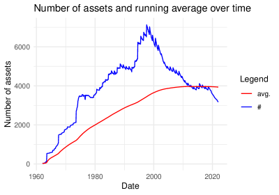
Figure 1: Size of cross section. The blue line # shows the number of assets over time. The red line shows a running average. The data are excess returns from common stocks from the year 1963 until 2021 from the CRSP data base.
Figure 1 shows the number of stocks in the sample (in blue), and the running average number of stocks (in red) remaining in the sample after applying the filters described above. At the start of the sample, there are multiple months with no more than thirty excess returns. There is a peak in the years preceding the year 2000. The running average at the end of the sample is around 4 000 stocks per month.
We parameterize the hypothesis space
by four different kernels, cosine and inverse multi-quadric (see Schölkopf and
Smola, 2018), Gaussian and Laplace (see Rasmussen and
Williams, 2005),
The cosine kernel is a finite-dimensional, correlation kernel, without hyper parameters. The second is the Gaussian kernel, with , of an infinite-dimensional space of smooth and rapidly decaying functions. The Laplace kernel, with , also defines an infinite-dimensional space of functions, as does the inverse multiquadric kernel for . For we use the simplest possible specification from Example 3.3, such that the idiosyncratic part of the covariance function becomes .
For the systematic part, we follow the low-rank framework from Section 2 using maximal ranks . We estimate that for the full specification is computationally intensive, but still feasible with moderate computational means.
For the parameter matrix , we thus need to estimate parameters. In addition to the length scales ,
we lower-bound the smallest eigenvalue of with , and validate this parameter together with the kernel parameters, if any. We set both regularization parameters , as the low-rank framework described in Section 2 already induces sparsity. For a model trained including returns , we validate the hyper parameters through a statistical scoring rule proposed by Dawid and
Sebastiani (1999),
(20)
as , where we make use of the Woodbury formula,
exploiting that is diagonal and full-rank. We additionally use the Sylvester (1851) formula to evaluate the determinant in (20) efficiently,
The following sections detail the empirical results obtained from these estimates. In Section 5.1, we first investigate how well the conditional moment model predicts the corresponding realizations. Subsequently, we consider empirical asset pricing implications in Section 5.2.
5.1 Predictive power of the conditional expectation model
If possesses full column rank , as a consequence of the low-rank algorithm, the conditional factor mean . We first assess the quality of the conditional moment estimates by comparing the low-dimensional moment matrix model to realizations. For first moments, an out-of-sample test statistic is obtained via predictive
(21)
where the competing model is the zero prediction. Note that the parameter in (21) carries a subscript, as the training and validation windows are rolled forward, and the estimated parameters change over time.
The joint presence of conditional moments of orders zero, one, and two, requires additional considerations on how to test the model beyond the commonly used predictive measures above for return expectations. In the statistics literature, this problem has been tackled by Dawid and
Sebastiani (1999), who propose a number of loss functions that are designed precisely for this goal. For a model trained up to, and including, the return vector , we use the scoring rule (20) to test the model, through evaluating out-of-sample.
(a)Cosine kernel
(b)Gauss kernel
(c)Laplace kernel
(d)Inverse multi-quadric kernel
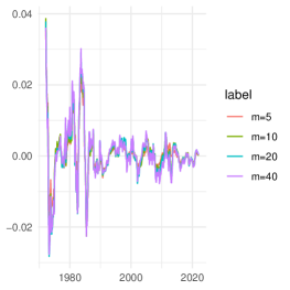
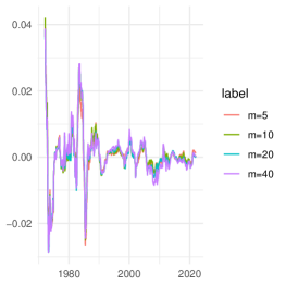
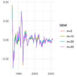
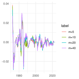
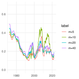
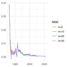
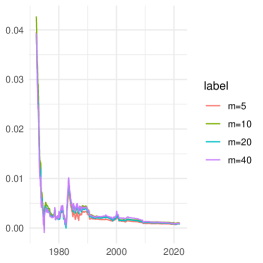
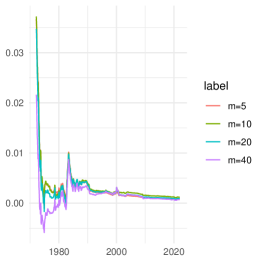
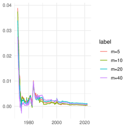
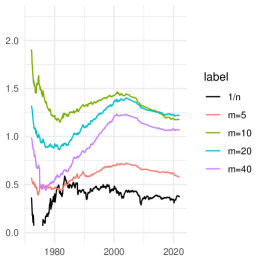
Figure 2: Predictive out-of-sample . The panels show rolling (over months) from (21) using the model proposed in this paper for . The underlying data are unbalanced US common stock excess returns and their characteristics from 1962 until 2021.
Figure 2 shows out-of-sample predictability results for the entire cross section. The measure shows to be highly persistent with on average slightly positive as evidenced by the expanding results in Figure 9. The lower- specifications tend to perform slightly worse than the higher- ones. There are no major differences between the different kernel specifications.
(a)Cosine kernel
(b)Gauss kernel
(c)Laplace kernel
(d)Inverse multi-quadric kernel
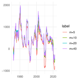
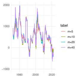
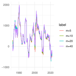
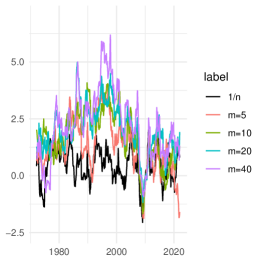
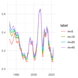
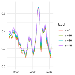
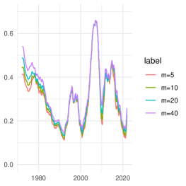
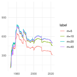
Figure 3: Scoring rules. The panels show the rolling (over months) average of out-of-sample excess loss differential , where the first summand arises from the model proposed in this paper, for , and the second from the specification (22). Both models are validated out-of-sample using unbalanced US stocks and their characteristics from 1962 until 2021.
Finally, we present results of a joint assessment of first and second moments that in this paper are proposed to be estimated jointly and consistently for unbalanced panels. With no competing nonparametric model for joint first and second conditional moments of unbalanced panels in the literature that we could test against the proposal of this paper, a zero-mean constant covariance contender is
(22)
where the parameter is validated through scoring rule (20) through loss function , and then tested out-of-sample as the realized loss .
We then introduce the scoring loss differential
where the loss function is defined in (20), and the competing conditional first and second moments are defined in model (22).
Figure 3 shows that the moment model developed in this paper dominates the constant model (22) for most time periods. This is a strong indication that there is statistical value in the nonparametric model. Empirical evidence over expanding windows in Figure 10 confirms this assessment. In summary, the evidence hints at higher-factor models producing a better fit.
With this section justifying statistically the factor model proposed in this paper, the next section investigates its asset pricing implications.
5.2 Asset pricing implications
With a model for conditional moments and a natural factor representation at hand that performs well in statistical terms, it is natural to employ it in an out-of-sample of portfolio exercise. It is well-documented in the literature that mean-variance efficient portfolios tend to underperform out-of-sample (Basak
et al., 2009), and even underperform portfolios. Both observations may well be a result of poorly estimated conditional moments.
Below, we reconsider the conditional mean-variance efficient portfolio problem using the estimated conditional means and covariances proposed in this paper. For this purpose, the full-rank covariance matrix model developed in Section 2 proves useful.
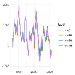
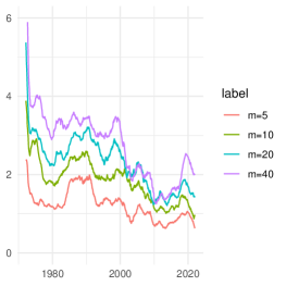
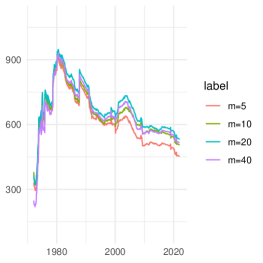
Figure 4 leads into the study of conditionally mean-variance efficient portfolios by showing the time series of the Hansen-Jagannathan bound generated by maximal Sharpe ratio portfolios for the different kernels used in this study. All panels confirm the natural ranking of higher maximal Sharpe ratio for higher uniformly across all data points. The levels generated by different kernels are comparable, with peaks reaching an annualized maximal Sharpe ratio of 6 for the cosine kernel for . The smallest predicted maximal Sharpe ratio is around one for . The depicted conditional Sharpe ratios are predictions by the models. We now investigate how these predictions translate into actual, realized Sharpe ratios.
(a)Cosine kernel
(b)Gauss kernel
(c)Laplace kernel
(d)Inverse multi-quadric kernel
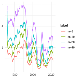
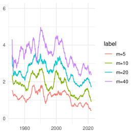
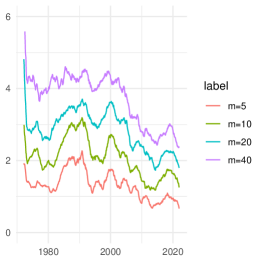
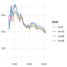
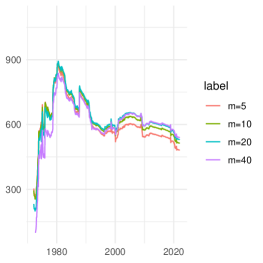
Figure 4: Predicted conditional Sharpe ratios. The panels show the rolling (over months) estimate of unconditional monthly out-of-sample portfolio Sharpe ratios over time. Mean-variance efficient portfolios use the solution proposed in this paper for and out-of-sample conditional covariance and conditional mean estimates. The data are unbalanced US stocks and their characteristics from 1962 until 2021.
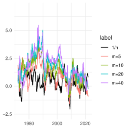
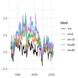
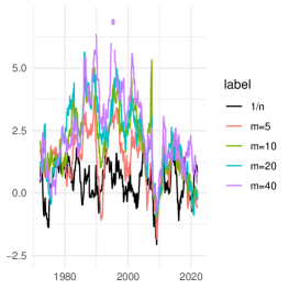
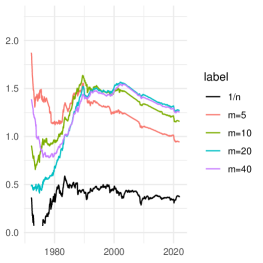
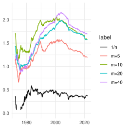
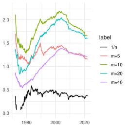
Figure 5 shows rolling estimators of unconditional monthly annualized Sharpe ratios over time along with those generated by portfolios. Generally, higher-factor models produce higher Sharpe ratio estimates. The magnitude of Sharpe ratios is considerable, with peaks beyond five for the Gaussian, and the inverse multiquadric model. Remarkably, this Sharpe ratio is generated despite only modest evidence of predictability of first moments, illustrating the quality of the joint estimates of first and second moments indicated already through the scoring rule in Figure 3. Sharpe ratios of portfolios are lower than the model-implied ones, and appear unrelated to them. Figure 11 shows Sharpe ratios estimated over expanding data points as uniformly positive at the end of the sample, some of which generate annualized values up to 1.75 for the Gaussian kernel. Considering this expanding evidence, it is not obvious to identify a dominating number of factors. However, over all kernels, the specification performs the worst, but is still well above the portfolio. Note that from factor spanning, the empirical Sharpe ratios of the factor portfolios are identical to the ones from the entire cross section. We therefore do not report these figures here.
(a)Cosine kernel
(b)Gauss kernel
(c)Laplace kernel
(d)Inverse multi-quadric kernel
Figure 5: Mean-variance portfolio Sharpe ratios. The panels show the rolling (over months) estimate of unconditional monthly out-of-sample portfolio Sharpe ratios over time. Mean-variance efficient portfolios use the solution proposed in this paper for and out-of-sample conditional covariance and conditional mean estimates. The data are unbalanced US stocks and their characteristics from 1962 until 2021.
With substantial empirical Sharpe ratios documented,
decomposition (3) raises the natural question about the amount of explanatory power contributed from systematic, and idiosyncratic risk, respectively. For this purpose, we calculate the ratio of systematic to total variance . Figure 6 shows that in the financial crisis in 2008, systematic risk is at an all time high at over 60%. Also during the Asian crisis in 1997 and the European devt crisis, the ratio goes well beyond 40%. Interestingly, none of the models show a high level of systematic risk during the COVID crisis starting in 2020, however.
(a)Cosine kernel
(b)Gauss kernel
(c)Laplace kernel
(d)Inverse multi-quadric kernel
Figure 6: Systematic and idiosyncratic risks. The panels show a rolling moving average calculated over months of as a measure for systematic to total risk for . The underlying data are unbalanced US stocks and their characteristics from 1962 until 2021.
Finally, one may be interested in the relation of the maximal Sharpe ratio portfolio and conventional asset pricing factors, such as the Fama and
French (2015) five factors that create exposure to size, value, profitability, and investment patterns, on top of the market portfolio. To this end, we estimate a contemporaneous regression of the out-of-sample maximal Sharpe ratio portfolio on the Fama-French five factors.
Tables 1 and 2 show that for all kernels and for , the intercept is highly significant. The market portfolio loads significantly loading across the cosine and Laplace specifications, less so for the Gaussian and inverse multi-quadric kernels. The CMA factor, the difference between
returns on diversified portfolios of the stocks of low and
high investment firms, also features for all kernels for . The dependence decreases for . Across all considered specifications, higher diminishes the explanatory power of the Fama-French five factors for the maximum Sharpe ratio portfolio.
m=5
m=10
m=20
m=40
(Intercept)
Mkt
SMB
HML
RMW
CMA
Adj. R2
; ;
(a)Cosine kernel
m=5
m=10
m=20
m=40
(Intercept)
Mkt
SMB
HML
RMW
CMA
Adj. R2
; ;
(b)Gaussian kernel
Table 1: Fama-French 5 factors and maximum Sharpe ratio SDF. The table shows results from a contemporaneous regression of the out-of-sample minimum-variance stochastic discount factor on the Fama and
French (2015) five factors. The top panel 7(a) shows the regression results from the cosine kernel, the bottom panel 7(b) from the Gaussian kernel. The underlying data are unbalanced US common stock excess returns and their characteristics from 1962 until 2021.
m=5
m=10
m=20
m=40
(Intercept)
Mkt
SMB
HML
RMW
CMA
Adj. R2
; ;
(a)Laplace kernel
m=5
m=10
m=20
m=40
(Intercept)
Mkt
SMB
HML
RMW
CMA
Adj. R2
; ;
(b)Inverse multi-quadric kernel
Table 2: Fama-French 5 factors and maximum Sharpe ratio SDF. The table shows results from a contemporaneous regression of the out-of-sample minimum-variance stochastic discount factor on the Fama and
French (2015) five factors. The top panel 8(a) shows the regression results from the cosine kernel, the bottom panel 8(b) from the Gaussian kernel. The underlying data are unbalanced US common stock excess returns and their characteristics from 1962 until 2021.
6 Conclusion
We propose a tractable nonparametric model for conditional first and second moments of unbalanced panels and prove its consistency and provide finite-sample guarantees. For all states of the world, these conditional first and second moments produce symmetric and positive semidefinite conditional covariance matrices. The model is formulated in terms of potentially infinite-dimensional hypothesis spaces that yield a precise and computable prescription of the conditional mean and covariance functions that are shown in Kozak and
Nagel (2024) to characterize the existence of a low-dimensional factor model that spans a high-dimensional cross section. We show that the model can be estimated efficiently and rapidly through the solution of a convex optimization problem with unique optimal solution, and thus lends itself to reproducible large-scale empirical studies.
We estimate the model (using an ordinary personal computer) on a large panel of US stock returns starting from the year 1962 until the end of 2021, using the stocks’ characteristics to modulate the time-varying conditional expected returns and covariances. The proposed model shows good properties with respect to a statistical scoring rule. It generates sizable out-of-sample Sharpe ratios far beyond those of equal-weighted portfolios.
Appendix A Incomplete pivoted Cholesky decomposition
Figure 9: Out-of-sample . The panels show out-of-sample from (21) using the model proposed in this paper for . The underlying data are unbalanced US common stock excess returns and their characteristics from 1962 until 2021.
(a)Cosine kernel
(b)Gauss kernel
(c)Laplace kernel
(d)Inverse multi-quadric kernel
Figure 10: Scoring rules. The panels show the running average of out-of-sample excess loss differential , where the first loss arises from the model proposed in this paper, for , and the second from the specification (22). Both models are validated out-of-sample using unbalanced US stocks and their characteristics from 1962 until 2021.
(a)Cosine kernel
(b)Gauss kernel
(c)Laplace kernel
(d)Inverse multi-quadric kernel
Figure 11: Mean-variance portfolio Sharpe ratios. The panels show the running estimate of unconditional out-of-sample portfolio Sharpe ratios over time. Mean-variance efficient portfolios use the solution proposed in this paper for and out-of-sample conditional covariance and conditional mean estimates. The data are unbalanced US stocks and their characteristics from 1962 until 2021.
References
Basak
et al. (2009)Basak, G. K., R. Jagannathan, and T. Ma (2009): “Jackknife
Estimator for Tracking Error Variance of Optimal Portfolios,”
Management Science, 55, 990–1002.
Berlinet and
Thomas-Agnan (2004)Berlinet, A. and C. Thomas-Agnan (2004): Reproducing Kernel
Hilbert Spaces in Probability and Statistics, Boston, MA: Springer US,
1–54.
Chamberlain (1983)Chamberlain, G. (1983): “Funds, Factors, and Diversification
in Arbitrage Pricing Models,” Econometrica, 51, 1305–1323.
Chamberlain and
Rothschild (1983)Chamberlain, G. and M. Rothschild (1983): “Arbitrage, Factor
Structure, and Mean-Variance Analysis on Large Asset Markets,”
Econometrica, 51, 1281–1304.
Chen
et al. (2023)Chen, Y., E. N. Epperly, J. A. Tropp, and R. J. Webber (2023):
“Randomly pivoted Cholesky: Practical approximation of a kernel
matrix with few entry evaluations,” .
Cochrane (2011)Cochrane, J. H. (2011): “Presidential Address: Discount
Rates,” Journal of Finance, 66, 1047–1108.
Connor
et al. (2012)Connor, G., M. Hagmann, and O. Linton (2012): “EFFICIENT
SEMIPARAMETRIC ESTIMATION OF THE FAMA-FRENCH MODEL AND EXTENSIONS,”
Econometrica, 80, 713–754.
Dawid and
Sebastiani (1999)Dawid, A. P. and P. Sebastiani (1999): “Coherent dispersion
criteria for optimal experimental design,” The Annals of Statistics,
27, 65 – 81.
Drineas and
Mahoney (2005)Drineas, P. and M. W. Mahoney (2005): “On the Nyström
Method for Approximating a Gram Matrix for Improved Kernel-Based Learning,”
Journal of Machine Learning Research, 6, 2153–2175.
Engle
et al. (2019)Engle, R. F., O. Ledoit, and M. Wolf (2019): “Large Dynamic
Covariance Matrices,” Journal of Business & Economic Statistics, 37,
363–375.
Fama and
French (1993)Fama, E. F. and K. R. French (1993): “Common risk factors in
the returns on stocks and bonds,” Journal of Financial Economics, 33,
3–56.
Fama and
French (2015)
——— (2015): “A five-factor asset
pricing model,” Journal of Financial Economics, 116, 1–22.
Fama and
French (2019)
——— (2019): “Comparing Cross-Section
and Time-Series Factor Models,” Review of Financial Studies, 33,
1891–1926.
Fama and
MacBeth (1973)Fama, E. F. and J. D. MacBeth (1973): “Risk, Return, and
Equilibrium: Empirical Tests,” Journal of Political Economy, 81,
607–636.
Fan
et al. (2016)Fan, J., Y. Liao, and W. Wang (2016): “PROJECTED PRINCIPAL
COMPONENT ANALYSIS IN FACTOR MODELS,” The Annals of Statistics, 44,
219–254.
Filipović and
Schneider (2024)Filipović, D. and P. Schneider (2024): “Fundamental
properties of linear factor models,” Tech. rep., working paper, EPFL,
Universitá della Svizzera Italian, and SFI.
Fortin
et al. (2023a)Fortin, A.-P., P. Gagliardini, and O. Scaillet (2023a):
“Eigenvalue Tests for the Number of Latent Factors in Short
Panels*,” Journal of Financial Econometrics, nbad024.
Fortin
et al. (2023b)
——— (2023b): “Latent
Factor Analysis in Short Panels,” Working paper, University of Geneva, and
Universitá delle Svizzera italiana.
Freyberger
et al. (2020)Freyberger, J., A. Neuhierl, and M. Weber (2020): “Dissecting
Characteristics Nonparametrically,” Review of Financial Studies, 33,
2326–2377.
Gu
et al. (2020a)Gu, S., B. Kelly, and D. Xiu (2020a):
“Autoencoder asset pricing models,” Journal of Econometrics.
Gu
et al. (2020b)
——— (2020b): “Empirical
Asset Pricing via Machine Learning,” Review of Financial Studies, 33,
2223–2273.
Horn and
Johnson (1990)Horn, R. A. and C. R. Johnson (1990): Matrix analysis,
Cambridge: Cambridge University Press, corrected reprint of the 1985
original.
Kelly
et al. (2019)Kelly, B. T., S. Pruitt, and Y. Su (2019): “Characteristics
are covariances: A unified model of risk and return,” Journal of
Financial Economics, 134, 501–524.
Kozak and
Nagel (2024)Kozak, S. and S. Nagel (2024): “When Do Cross-Sectional Asset
Pricing Factors Span the Stochastic Discount Factor?” Working Paper 31275,
National Bureau of Economic Research.
Kozak
et al. (2020)Kozak, S., S. Nagel, and S. Santosh (2020): “Shrinking the
cross-section,” Journal of Financial Economics, 135, 271–292.
Milz (2023)Milz, J. (2023): “Sample average approximations of strongly
convex stochastic programs in Hilbert spaces,” Optim. Lett., 17,
471–492.
Paulsen and
Raghupathi (2016)Paulsen, V. I. and M. Raghupathi (2016): An introduction to the
theory of reproducing kernel Hilbert spaces, vol. 152 of Cambridge
Studies in Advanced Mathematics, Cambridge University Press, Cambridge.
Rasmussen and
Williams (2005)Rasmussen, C. E. and C. K. I. Williams (2005): Gaussian
Processes for Machine Learning, The MIT Press.
Reisman (1988)Reisman, H. (1988): “A General Approach to the Arbitrage
Pricing Theory (APT),” Econometrica, 56, 473–476.
Ross (1976)Ross, S. A. (1976): “The arbitrage theory of capital asset
pricing,” Journal of Economic Theory, 13, 341–360.
Schölkopf and
Smola (2018)Schölkopf, B. and A. J. Smola (2018): Learning with
Kernels: Support Vector Machines, Regularization, Optimization, and Beyond,
The MIT Press.
Shapiro et al. (2021)Shapiro, A., D. Dentcheva, and A. Ruszczyński (2021):
Lectures on stochastic programming—modeling and theory, vol. 28 of
MOS-SIAM Series on Optimization, Society for Industrial and Applied
Mathematics (SIAM), Philadelphia, PA; Mathematical Optimization Society,
Philadelphia, PA, third ed.
Sylvester (1851)Sylvester, J. (1851): “XXXVII. On the relation between the
minor determinants of linearly equivalent quadratic functions,” The
London, Edinburgh, and Dublin Philosophical Magazine and Journal of Science,
1, 295–305.
Welch and
Goyal (2008)Welch, I. and A. Goyal (2008): “A Comprehensive Look at The
Empirical Performance of Equity Premium Prediction,” Review of
Financial Studies, 21, 1455–1508.
Zaffaroni (2019)Zaffaroni, P. (2019): “Factor Models for Asset Pricing,”
Working paper, Imperial College.