Purely electrical detection of the Néel vector of -wave magnets
based on linear and nonlinear conductivities
Abstract
A -wave magnet has a momentum-dependent band structure and zero-net magnetization just as in the case of an altermagnet. It will be useful for high-density and ultra-fast memory. However, it is a nontrivial problem to detect the Néel vector of a -wave magnet because time-reversal symmetry is preserved, while this is not a problem in an altermagnet because the anomalous Hall conductivity may be present due to the breaking of time-reversal symmetry. Here, we show that it is possible to detect the in-plane component of the Néel vector of the -wave magnet by measuring the transverse and longitudinal Drude conductivity. Remarkably, this is possible without magnetization. Furthermore, it is possible to detect the -component by measuring nonlinear conductivity including the nonlinear Drude conductivity and quantum-metric induced nonlinear conductivity by introducing tiny magnetization along the axis. We obtain analytic formulae for them in the first-order perturbation theory, which agree quite well with numerical results without perturbation. Our results will pave a way to spintronic memory based on -wave magnets.
Introduction
Ferromagnets are useful for nonvolatile memories, where the up and down spins act as a bit. On the other hand, antiferromagnets are expected to act as more efficient memories owing to their zero net magnetization, where high-density and quick-switchable memories may be possible. However, it is very hard to readout the direction of the Néel vector of antiferromagnet[1, 2, 3, 4, 5, 6, 7]. Recently, altermagnets attract growing interests[8, 9, 10] because they have both merits of ferromagnets and antiferromagnets. Altermagnets have zero net magnetization and they break time-reversal symmetry. Accordingly, the Néel vector is observable by means of the anomalous Hall conductivity[11, 12, 13, 14]. A characteristic feature of altermagnets which is absent in both ferromagnets and antiferromagnets is the momentum-dependent band structure[15, 16, 17, 8, 9, 10], which includes the -wave, -wave and -wave band structures. Indeed, momentum dependent band structures have been observed by Angle-Resolved Photo-Emission Spectroscopy (ARPES)[18, 19, 20, 21, 22]. Furthermore, spin current is generated in -wave altermagnets[17, 23, 24, 25].
A -wave magnet was proposed only recently[26]. They have zero net magnetization as well. They resemble altemagnets from a point of view that they have momentum-dependent band structure with the -wave symmetry. However, they preserve time-reversal symmetry, which leads to the zero anomalous Hall conductivity. There is so far no known method to detect the Néel vector of -wave magnets, which makes difficult to use them for spintronics.
The linear conductivity is defined by , where is an applied electric field along the direction and is the current along the direction. They include the longitudinal Drude conductivity and the transverse Drude conductivity . On the other hand, there are several studies on nonlinear conductivity[27, 28, 29, 30, 31, 32, 33, 34, 35, 36, 37, 38, 39]. Especially, the second-order nonlinear conductivity is defined by , where is an applied electric field along the direction and is the current along the direction. Among them, the nonlinear Drude conductivity is proportional to , where is the electron relaxation time. It is an extrinsic nonlinear conductivity, while the quantum-metric induced nonlinear conductivity is intrinsic because it is irrelevant to .
In this paper, we show that the in-plane component of the Néel vector of -wave magnets is detectable by measuring the transverse and longitudinal linear Drude conductivities. Remarkably, this is possible without magnetization. In addition, the -component of the Néel vector of -wave magnets is detectable by measuring the nonlinear conductivity with the aid of the magnetization along the axis. We obtain analytic formulae for linear and nonlinear conductivities based on a perturbation theory with respect to the magnitude of the Néel vector and magnetization , which agree quite well with numerical results without perturbation.
Model
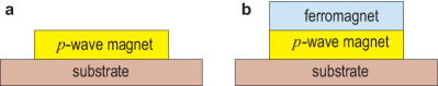
We analyze a system where a -wave magnet is placed on a substrate as shown in Fig.1a. The substrate breaks inversion symmetry and induces the Rashba interaction. Then, the Hamiltonian is given by
| (1) |
The first term represents the kinetic energy of free fermions
| (2) |
with , where is the free-fermion mass, and is identity matrix. The second term represents the Rashba interaction
| (3) |
where is the magnitude of the spin-orbit interaction, and and are the Pauli matrix for the spin. The third term
| (4) |
describes the effect of the -wave magnet[26, 40, 41] with the direction of the Néel vector , where is the magnitude of the -wave magnet, and is the Néel vector. Then, we have , and .
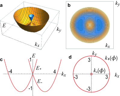
The band structure is shown in Fig.2, where the Néel vector is taken along the axis. A Dirac cone exists at the momentum as shown in Fig.2a, which is formed by the Rashba interaction. The Fermi surfaces have the -wave symmetry as shown in Fig.2b. There are two Fermi surfaces as shown in Fig.2d, where and .
Drude conductivity
We first study linear conductivities. We use a perturbation theory in assuming with . The longitudinal Drude conductivity is calculated based on Eq.(22) in Methods, as
| (5) |
for , and
| (6) |
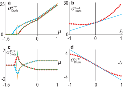
for . See the detailed derivation in Sec.II S1-1 of Supplementary Information. It is shown as a function of the chemical potential in Fig.3a and as a function of in Fig.3b. It has a dependence on the -component of the Néel vector. Hence, is detectable by means of the longitudinal linear Drude conductivity.
The transverse Drude conductivity is calculated as
| (7) |
for , and
| (8) |
for . See the detailed derivation in Sec.II S1-2 of Supplementary Information. It is proportional to the -component of the Néel vector. It is shown as a function of the chemical potential in Fig.3c and as a function of in Fig.3d. Hence, is also detectable by means of the transverse linear Drude conductivity.
Nonlinear longitudinal conductivity
We proceed to study nonlinear conductivities. In the following, we introduce magnetization, which is induced by attaching ferromagnet. We add the Hamiltonian
| (9) |
which describes the effect of magnetization as shown in Fig.1b. Instead, this term is introduced by applying external magnetic field. The breaking of time-reversal symmetry is necessary for nonzero nonlinear conductivities[37].
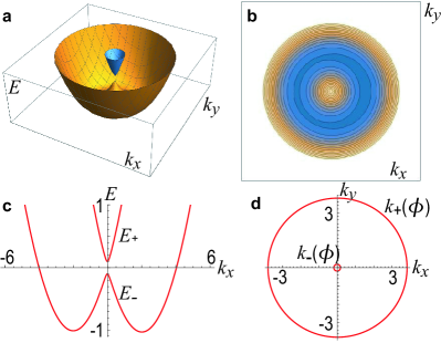
The band structure is shown in Fig.4, where the Néel vector is taken along the axis. A Dirac cone at the momentum has a gap with as shown in Fig.4a. There are two Fermi surfaces formed by the lower band for and formed by the lower band and the upper band for , while there is a Fermi surface formed by the lower band for as shown in Fig.4c.
We first study nonlinear longitudinal conductivity. There are two contributions. One is the nonlinear Drude conductivity and the other is the quantum-metric induced nonlinear conductivity. We use a perturbation theory in and assuming and . The nonlinear Drude conductivity at the chemical potential is analytically calculated based on Eq.(30) in Methods as
| (10) |
where for , and for . It is valid for . See the detailed derivation in Sec.III S1-1 of Supplementary Information. It is proportional to the -component of the Néel vector. On the other hand, the quantum-metric induced nonlinear conductivity is analytically obtained based on Eq.(25) in Methods as
| (11) |
for , and
| (12) |
for . See the detailed derivation in Sec.III S1-2 of Supplementary Information. It is also proportional to . Hence, is observable. The leading order of the nonlinear conductivity is proportional to , which means that magnetization is necessary to detect the -component of the Néel vector.
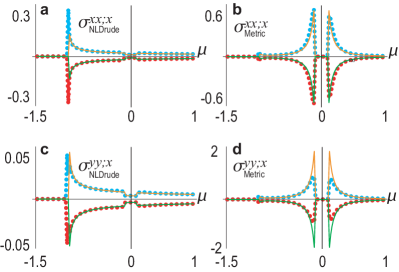
We show analytical results based on the perturbation theory and numerical results without using the perturbation theory. The nonlinear conductivity is shown as a function of the chemical potential in Fig.5. They agree with each other very well, which assures the validity of the perturbation theory. The nonlinear Drude conductivity diverges at the band bottom and its value becomes half inside of the bulk gap comparing with the outside of the bulk gap . On the other hand, the quantum-metric induced nonlinear conductivity diverges at the band edge and takes tiny value inside of the band gap . Therefore, two contributions are differentiated although the explicit value of is unknown.
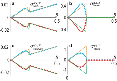
The nonlinear conductivities are shown as a function of in Fig.6. They show nonmonotonic behavior and there is a sudden jump at . It is because nonlinear conductivities depend on whether the chemical potential is outside of the band gap or inside of the band gap.
Nonlinear transverse conductivity
Next, we study nonlinear transverse conductivity. There are three contributions. Nonlinear Drude conductivity, the quantum-metric induced nonlinear conductivity and the Berry-curvature-dipole induced nonlinear conductivity. Explicit calculation shows that the Berry-curvature-dipole induced nonlinear conductivity is zero.
The nonlinear Drude conductivity at the chemical potential is analytically calculated based on Eq.(30) in Methods as
| (13) |
See the detailed derivation in Sec.III S2-1 of Supplementary Information. On the other hand, quantum-metric induced nonlinear conductivity is analytically obtained based on Eq.(25) as
| (14) |
for , and
| (15) |
for . See the detailed derivation in Sec.III S2-2 of Supplementary Information. Hence, we can also observe by measuring the nonlinear transverse conductivity. The behavior of the nonlinear transverse conductivity as a function of is similar to that of the nonlinear longitudinal conductivity.
Discussion
-wave magnets have zero-net magnetization, which may lead to a high-density and ultra-fast memory as in the case of antiferromagnets and altermagnets. We have found that the Néel vector of the in-plane component of the -wave magnet is detectable by the linear Drude conductivity without using magnetization. It is contrasted to the -wave altermagnet, where the Néel vector is not detectable by the linear Drude conductivity but the measurement of the nonlinear conductivity is necessary[46]. On the other hand, the -component of the Néel vector is detectable by measuring the nonlinear conductivity with the aid of magnetization.
Our results will pave a way to spintronic memory based on -wave magnets. For example, the -wave magnet may have easy-axis anisotropy along the axis if we make a one-dimensional sample along the axis. Then, the Néel vector points along the axis, which acts as an Ising variable and can be used for a binary memory. It is detectable by measuring the linear Drude conductivity.
Methods
The energy spectrum of the Hamiltonian (1) is given by
| (16) |
where
| (17) | ||||
| (18) | ||||
| (19) |
We introduce the polar coordinate and . In the first order of and , the energy is expanded as
| (20) |
The Fermi surfaces for the lower band are obtained as
| (21) |
The Drude conductivity is given by the formula[42]
| (22) |
where is the Fermi distribution function for the band , and is the chemical potential.
The second-order nonlinear conductivity is expanded in terms of the electron relaxation time as[37]
| (23) |
where
| (24) |
First, only the term survives in the dirty limit , which is the intrinsic nonlinear conductivity. It is the quantum-metric induced nonlinear conductivity given by[37]
| (25) |
where is the band–energy normalized quantum metric or the Berry connection polarizability. It is given as[27, 29, 32, 36, 37, 43]
| (26) |
with being the energy of the band , and being the interband Berry connection
| (27) |
Second, is the nonlinear transverse conductivity induced by the Berry curvature dipole[28],
| (28) |
with the Berry curvature
| (29) |
It is an extrinsic nonlinear conductivity, since it vanishes as .
Third, is the nonlinear Drude conductivity[44],
| (30) |
where is the energy of the band . It is also an extrinsic nonlinear conductivity.
This work is supported by CREST, JST (Grants No. JPMJCR20T2) and Grants-in-Aid for Scientific Research from MEXT KAKENHI (Grant No. 23H00171).
References
- [1] T. Jungwirth, X. Marti, P. Wadley and J. Wunderlich, Antiferromagnetic spintronics, Nature Nanotechnology 11, 231 (2016).
- [2] V. Baltz, A. Manchon, M. Tsoi, T. Moriyama, T. Ono, and Y. Tserkovnyak, Antiferromagnetic spintronics, Rev. Mod. Phys. 90, 015005 (2018).
- [3] Jiahao Han, Ran Cheng, Luqiao Liu, Hideo Ohno and Shunsuke Fukami, Coherent antiferromagnetic spintronics, Nature Materials 22, 684 (2023).
- [4] Zhuoliang Ni, A. V. Haglund, H. Wang, B. Xu, C. Bernhard, D. G. Mandrus, X. Qian, E. J. Mele, C. L. Kane and Liang Wu , Imaging the Neel vector switching in the monolayer antiferromagnet MnPSe3 with strain-controlled Ising order, Nature Nanotechnology 16, 782 (2021).
- [5] J. Godinho, H. Reichlov, D. Kriegner, V. Novak, K. Olejnik, Z. Kašpar, Z. Šoban, P. Wadley, R. P. Campion, R. M. Otxoa, P. E. Roy, J. Železnny, T. Jungwirth and J. Wunderlich, Electrically induced and detected Neel vector reversal in a collinear antiferromagnet, Nature Communications volume 9, Article number: 4686 (2018).
- [6] Kenta Kimura, Yutaro Otake and Tsuyoshi Kimura, Visualizing rotation and reversal of the Neel vector through antiferromagnetic trichroism, Nature Communications, 13, 697 (2022).
- [7] Yi-Hui Zhang, Tsao-Chi Chuang, Danru Qu, and Ssu-Yen Huang, Detection and manipulation of the antiferromagnetic Neel vector in Cr2O3 Phys. Rev. B 105, 094442 (2022).
- [8] L. Smejkal, A. H. MacDonald, J. Sinova, S. Nakatsuji and T. Jungwirth, Anomalous Hall antiferromagnets, Nat. Rev. Mater. 7, 482 (2022).
- [9] L. Smejkal, J. Sinova, and T. Jungwirth, Beyond Conventional Ferromagnetism and Antiferromagnetism: A Phase with Nonrelativistic Spin and Crystal Rotation Symmetry, Phys. Rev. X, 12, 031042 (2022).
- [10] Libor Šmejkal, Jairo Sinova, and Tomas Jungwirth, Emerging Research Landscape of Altermagnetism, Phys. Rev. X 12, 040501 (2022).
- [11] Amar Fakhredine, Raghottam M. Sattigeri, Giuseppe Cuono, and Carmine Autieri, Interplay between altermagnetism and nonsymmorphic symmetries generating large anomalous Hall conductivity by semi-Dirac points induced anticrossings, Phys. Rev. B 108, 115138 (2023).
- [12] Teresa Tschirner, Philipp Keler, Ruben Dario Gonzalez Betancourt, Tommy Kotte, Dominik Kriegner, Bernd Buechner, Joseph Dufouleur, Martin Kamp, Vedran Jovic, Libor Smejkal, Jairo Sinova, Ralph Claessen, Tomas Jungwirth, Simon Moser, Helena Reichlova, Louis Veyrat, Saturation of the anomalous Hall effect at high magnetic fields in altermagnetic RuO2, APL Mater. 11, 101103 (2023)
- [13] Toshihiro Sato, Sonia Haddad, Ion Cosma Fulga, Fakher F. Assaad, Jeroen van den Brink, Altermagnetic anomalous Hall effect emerging from electronic correlations, Phys. Rev. Lett. 133, 086503 (2024)
- [14] Miina Leivisk Javier Rial, Anton Badura, Rafael Lopes Seeger, Ismaa Kounta, Sebastian Beckert, Dominik Kriegner, Isabelle Joumard, Eva Schmoranzerov Jairo Sinova, Olena Gomonay, Andy Thomas, Sebastian T. B. Goennenwein, Helena Reichlov Libor Smejkal, Lisa Michez, Tom Jungwirth, Vincent Baltz, Anisotropy of the anomalous Hall effect in the altermagnet candidate Mn5Si3 films, Phys. Rev. B 109, 224430 (2024)
- [15] K.-H. Ahn, A. Hariki, K.-W. Lee, and J. Kunes, Antiferromagnetism in RuO2 as d-wave Pomeranchuk instability, Phys. Rev. B 99, 184432 (2019).
- [16] S. Hayami, Y. Yanagi, and H. Kusunose, Momentum-Dependent Spin Splitting by Collinear Antiferromagnetic Ordering, J. Phys. Soc. Jpn. 88, 123702 (2019).
- [17] Makoto Naka, Satoru Hayami, Hiroaki Kusunose, Yuki Yanagi, Yukitoshi Motome and Hitoshi Seo, Spin current generation in organic antiferromagnets, Nat. Com. 10, 4305 (2019).
- [18] J. Krempask, L. Šmejkal, S. W. D’Souza, M. Hajlaoui, G. Springholz, K. Uhlov F. Alarab, P. C. Constantinou, V. Strocov, D. Usanov, W. R. Pudelko, R. Gonzez-Herndez, A. Birk Hellenes, Z. Jansa, H. Reichlov Z. Šob, R. D. Gonzalez Betancourt, P. Wadley, J. Sinova, D. Kriegner, J. Min, J. H. Dil and T. Jungwirth, Altermagnetic lifting of Kramers spin degeneracy, Nature 626, 517 (2024).
- [19] Suyoung Lee, Sangjae Lee, Saegyeol Jung, Jiwon Jung, Donghan Kim, Yeonjae Lee, Byeongjun Seok, Jaeyoung Kim, Byeong Gyu Park, Libor Šmejkal, Chang-Jong Kang, Changyoung Kim, Broken Kramers Degeneracy in Altermagnetic MnTe, Phys. Rev. Lett. 132, 036702 (2024).
- [20] O. Fedchenko, J. Minar, A. Akashdeep, S.W. D’Souza, D. Vasilyev, O. Tkach, L. Odenbreit, Q.L. Nguyen, D. Kutnyakhov, N. Wind, L. Wenthaus, M. Scholz, K. Rossnagel, M. Hoesch, M. Aeschlimann, B. Stadtmueller, M. Klaeui, G. Schoenhense, G. Jakob, T. Jungwirth, L. Smejkal, J. Sinova, H. J. Elmers, Observation of time-reversal symmetry breaking in the band structure of altermagnetic RuO2, Science Advances 10,5 (2024) DOI: 10.1126/sciadv.adj4883.
- [21] T. Osumi, S. Souma, T. Aoyama, K. Yamauchi, A. Honma, K. Nakayama, T. Takahashi, K. Ohgushi, and T. Sato, Observation of a giant band splitting in altermagnetic MnTe, Phys. Rev. B 109, 115102 (2024)
- [22] Zihan Lin, Dong Chen, Wenlong Lu, Xin Liang, Shiyu Feng, Kohei Yamagami, Jacek Osiecki, Mats Leandersson, Balasubramanian Thiagarajan, Junwei Liu, Claudia Felser, Junzhang Ma, Observation of Giant Spin Splitting and d-wave Spin Texture in Room Temperature Altermagnet RuO2, arXiv:2402.04995.
- [23] Rafael Gonzalez-Hernandez, Libor Šmejkal, Karel Vborn, Yuta Yahagi, Jairo Sinova, Tomš Jungwirth, and Jakub Železn, Efficient electrical spin splitter based on nonrelativistic collinear antiferromagnetism, Phys. Rev. Lett., 126:127701, (2021).
- [24] M Naka, Y Motome, and H Seo, Perovskite as a spin current generator. Phys. Rev. B, 103, 125114, (2021).
- [25] Arnab Bose, Nathaniel J. Schreiber, Rakshit Jain, Ding-Fu Shao, Hari P. Nair, Jiaxin Sun, Xiyue S. Zhang, David A. Muller, Evgeny Y. Tsymbal, Darrell G. Schlom & Daniel C. Ralph, Tilted spin current generated by the collinear antiferromagnet ruthenium dioxide, Nature Electronics 5, 267 (2022).
- [26] Anna Birk Hellenes, Tomas Jungwirth, Jairo Sinova, Libor Šmejkal, Unconventional p-wave magnets, arXiv:2309.01607.
- [27] Y. Gao, S. A. Yang, and Q. Niu, Field induced positional shift of Bloch electrons and its dynamical implications, Phys. Rev. Lett. 112, 166601 (2014).
- [28] I. Sodemann and L. Fu, Quantum nonlinear Hall effect induced by Berry curvature dipole in time-reversal invariant materials, Phys. Rev. Lett. 115, 216806 (2015).
- [29] H. Liu, J. Zhao, Y.-X. Huang, W. Wu, X.-L. Sheng, C. Xiao, and S. A. Yang, Intrinsic second-order anomalous Hall effect and its application in compensated antiferromagnets, Phys. Rev. Lett. 127, 277202 (2021).
- [30] Y. Michishita and N. Nagaosa, Dissipation and geometry in nonlinear quantum transports of multiband electronic systems, Phys. Rev. B 106, 125114 (2022).
- [31] H. Watanabe and Y. Yanase, Nonlinear electric transport in odd-parity magnetic multipole systems: Application to Mn-based compounds, Phys. Rev. Res. 2, 043081 (2020).
- [32] C. Wang, Y. Gao, and D. Xiao, Intrinsic nonlinear Hall effect in antiferromagnetic tetragonal cumnas, Phys. Rev. Lett. 127, 277201 (2021).
- [33] R. Oiwa and H. Kusunose, Systematic analysis method for nonlinear response tensors, J. Phys. Soc. Jpn. 91, 014701 (2022).
- [34] A. Gao, Y.-F. Liu, J.-X. Qiu, B. Ghosh, T.V. Trevisan, Y. Onishi, C. Hu, T. Qian, H.-J. Tien, S.-W. Chen et al., Quantum metric nonlinear Hall effect in a topological antiferromagnetic heterostructure, Science 381, eadf1506 (2023).
- [35] N. Wang, D. Kaplan, Z. Zhang, T. Holder, N. Cao, A. Wang, X. Zhou, F. Zhou, Z. Jiang, C. Zhang et al., Quantum metric-induced nonlinear transport in a topological antiferromagnet, Nature 621, 487 (2023).
- [36] Kamal Das, Shibalik Lahiri, Rhonald Burgos Atencia, Dimitrie Culcer, and Amit Agarwal, Intrinsic nonlinear conductivities induced by the quantum metric, Phys. Rev. B 108, L201405 (2023).
- [37] Daniel Kaplan, Tobias Holder and Binghai Yan, Unification of Nonlinear Anomalous Hall Effect and Nonreciprocal Magnetoresistance in Metals by the Quantum Geometry, Phys. Rev. Lett. 132, 026301 (2024).
- [38] YuanDong Wang, ZhiFan Zhang, Zhen-Gang Zhu, and Gang Su, Intrinsic nonlinear Ohmic current, Phys. Rev. B 109, 085419 (2024).
- [39] Longjun Xiang, Bin Wang, Yadong Wei, Zhenhua Qiao, and Jian Wang, Linear displacement current solely driven by the quantum metric, Phys. Rev. B 109, 115121 (2024).
- [40] Kazuki Maeda, Bo Lu, Keiji Yada, Yukio Tanaka, Theory of tunneling spectroscopy in p-wave altermagnet-superconductor hybrid structures, J. Phys. Soc. Jpn. 93, 114703 (2024).
- [41] M. Ezawa, Topological insulators based on -wave altermagnets; Electrical control and detection of the altermagnetic domain wall, Phys. Rev. B 110, 165429 (2024).
- [42] Yuan Fang, Jennifer Cano, and Sayed Ali Akbar Ghorashi, Quantum Geometry Induced Nonlinear Transport in Altermagnets, Phys. Rev. Lett. 133, 106701 (2024).
- [43] Maria Teresa Mercaldo, Mario Cuoco, and Camine Ortix, Nonlinear planar magnetotransport as a probe of the quantum geometry of topological surface states, arXiv:2408.09543.
- [44] D. Kaplan, T. Holder, and B. Yan, Unifying semiclassics and quantum perturbation theory at nonlinear order, SciPost Phys. 14, 082 (2023).
- [45] T. Ideue, K. Hamamoto, S. Koshikawa, M. Ezawa, S. Shimizu, Y. Kaneko, Y. Tokura, N. Nagaosa, and Y. Iwasa, Bulk rectification effect in a polar semiconductor, Nat. Phys. 13, 578 (2017).
- [46] M. Ezawa. Detecting the Neel vector of altermagnets in heterostructures with a topological insulator and a crystalline valley-edge insulator, Physical Review B 109 (24), 245306 (2024).