Integrability properties and multi-kink solutions
of a generalised Fokker-Planck equation
Abstract
We analyse a generalised Fokker-Planck equation by making essential use of its linearisability through a Cole-Hopf transformation. We determine solutions of travelling wave and multi-kink type by resorting to a geometric construction in the regime of small viscosity. The resulting asymptotic solutions are time-dependent Heaviside step functions representing classical (viscous) shock waves. As a result, line segments in the space of independent variables arise as resonance conditions of exponentials and represent shock trajectories. We then discuss fusion and fission dynamics exhibited by the multi-kinks by drawing parallels in terms of shock collisions and scattering processes between particles, which preserve total mass and momentum. Finally, we propose Bäcklund transformations and examine their action on the solutions to the equation under study.
Keywords: C-integrable nonlinear PDEs, conservation laws, Fokker-Planck equations, multi-kinks, shock-particle duality, Bäcklund transformations.
1 Introduction
Models expressed by conservation laws and nonlinear partial differential equations (PDEs) play a crucial role in a number of fields, ranging from fluid dynamics [1] and condensed matter physics [2] to population dynamics [3] and social sciences [4], and to chemical systems [5]. Paradigmatic examples are provided by pivotal nonlinear PDEs with diffusion that have attracted huge attention in past decades, such as the Bateman-Burgers equation , or more general nonlinear Fokker-Planck models , being the viscosity/diffusion coefficient. Indeed, these models very naturally arise while dealing with the mean field approximation of many-body systems [6], incorporating various significant phenomena such as phase transitions, travelling-wave solutions, shock waves, and anomalous diffusion.
In this paper, we address the study of a nonlinear partial differential equation that can be considered a generalisation of the aforementioned models, that is
| (1.1) |
where is a real function of the two real independent variables and , is thought to be a small positive parameter, and and the ’s are real constants. This equation has been introduced recently in [7] in connection with the problem of describing fluid systems of volume whose behaviour at pressure and temperature deviates from the van der Waals equations of state. However, its potential applicability is far more general, in principle. Indeed, Equation (1.1) is basically a conservation law, albeit not in a familiar evolutionary form , for which many general results are available in the literature (see e.g. [8, 9, 10, 11, 12]). As a matter of fact, (1.1) belongs to the family of continuity equations of the form . Compared to standard nonlinear Fokker-Planck models, more drift and diffusion mechanisms are accounted. Expressly for Eq. (1.1), one recovers indeed the current , with and . Accordingly, Eq. (1.1) can be seen as a generalised Fokker-Planck equation whose structure is of the type
| (1.2) |
where , . Remark that for an equation of the Bateman-Burgers type follows, which is a fundamental nonlinear PDE renowned for its complete integrability, due to its remarkable property of being linearisable by means of a Cole-Hopf transformation (see e.g. [9] and Refs. therein). Equation (1.1) may be also seen as a sort of variation of the Bateman-Burgers equation similar to the Benjamin-Bona-Mohoney model [13] in the dissipative case, or to other analogous PDEs.
There are several ways to approach the study of solutions to (1.1), and their classification based on their properties. For instance, one may consider what happens in the inviscid case as in [7, 14], where multivalued solutions replaced by shock-type discontinuities have been evidenced [7]. Moreover, one may investigate the symmetries of the equation within a Lie-group framework to characterise analytically the similarity solutions on symmetry group orbits, as in [15], where attention has been also paid on pole dynamics by resorting to standard procedures. First in [7, 14], then more recently in [15], several special classes of solutions have been therefore considered that show rich dynamics and phenomenology. Nevertheless, additional questions can still be raised paving the way for achieving a clearer and broader perspective.
In the present work, we continue the analysis of Eq. (1.1) unveiling novel features of its solutions and its integrability structure. To do so, we will pay our attention to the key-property of Eq. (1.1), that is its linearisability via a Cole-Hopf type transformation [7]. Such property, although being strongly motivating in the original derivation of the equation, has indeed received limited attention thus far in respect to potential implications and applications. From the integrable systems perspective, this means that Eq. (1.1) is an analogous of the Bateman-Burgers equation, suggesting that the problem (1.1) may exhibit a plethora of integrability properties [16]. Thus, it is certainly helpful to assess Eq. (1.1) against techniques commonly employed to determine special classes of solutions to the Bateman-Burgers or other diffusive equations. One of such techniques is the Hirota bilinear method, which plays an important role in solving nonlinear integrable PDEs, see e.g. [17, 18], unveiling often the existence of multi-soliton solutions. The existence of Bäcklund transformations for Eq. (1.1) may be devised too, thus enhancing the analysis of its solutions and integrability properties. By making use of the Hirota method and Bäcklund transformations, we will identify soliton solutions of multi-kink type to Eq. (1.1), which are underpinned by the implementation of suitable nonlinear superposition formulae.
The paper is organised as follows. In Section 2, we discuss some features of Equation (1.1), by identifying two distinguished scalings, depending on conditions for the coefficients . In Section 3, we derive travelling wave solutions for the two equations implied by the scalings, and highlight their dynamical features. In Section 4, we tackle the problem of finding multi-kink solutions and carefully detail preeminent questions implied in their dynamics. We show the formation of classical (viscous) shocks, whose trajectories are provided by resonance conditions, and identify mass and momentum conservation laws. This allows us to describe the interaction among shocks in terms of scattering among particles, establishing an intriguing shock-particle duality. Section 5 is devoted to Bäcklund transformations (BTs). We prospectively devise one- and two-parameters BTs and analyse their action on an initial solution. We show explicitly how BTs for Eq. (1.1) generate new travelling components, which add to seed solution of the form derived in Section 2. Section 6 is devoted to discussion and conclusions.
2 Symmetries and rescalings
Equation (1.1) contains six phenomenological parameters whose individual values have to be fixed pertaining the specific problem to be addressed. In this section, we perform scalings on variables and coefficients to simplify the analysis of Eq. (1.1) and better comprehend special cases and limits. For instance, we can take into account the two classical limits i) and ii) below.
-
i)
The inviscid (dispersionless) limit and , from which, along with the rescaling , one obtains a Riemann-Hopf type equation
(2.3) Equation (2.3) admits the general solution implicitly expressed by the hodograph transformation
(2.4) where the arbitrary function determines the initial data for the implicit solution , and then its singularities, which propagates at the characteristic velocity
Remarkably, the non trivial dependency on of is determined by the structural parameter of the model
(2.5) In fact, when vanishes, one merely has that the initial datum propagates at the constant speed . This suggest that in several circumstances it is useful to perform the Galilei transformation
(2.6) -
ii)
The limit and which, combined with the time scaling provides the Bateman-Burgers equation with representing the effective viscosity.
The previous two limits commute, leading to the Riemann-Hopf equation . Moreover, it is well-known that the integrability properties of the two type of equations relies on the existence of infinitely many commuting flows, or symmetries. In the inviscid case, Eq. (2.3) commutes with any flows described by similar equations of the type for any differentiable function . On the other hand, also the Bateman-Burgers equation admits an infinite numerable set of commuting flows, recursively defined by [19]
| (2.7) |
where
| (2.8) |
and . The Bateman-Burgers equation corresponds to .
For what follows, it could be of some interest the limit of the Eq. (1.1). It yields
| (2.9) |
which in the inviscid limit provides again an equation of Riemann-Hopf type as in the Bateman-Burger case, but with a singular current. In this sense, the limit provides a class of equations qualitatively distinct from the Bateman-Burgers one. On the other hand, it is exactly for these models, obtained by the double limit , that one can interpret certain classes of solutions as equation of state for the van der Waals gases [7], as can be easily seen for particular choices of the function in (2.4).
For the general Eq. (1.1) one would like to verify whether it shares the beautiful set of properties possessed by the limit cases i) and ii) above. In doing this, by introduction of in (2.5) one already noticed that the whole space of the model parameters can be decomposed in two regions according to the two cases
| (2.10) |
Such a distinction is supported by the results concerning the point symmetries analysis of the Equation (1.1), signalling quite a relevant difference out the two cases [14]: there exists a finite algebra in the first case and an infinite dimensional symmetry algebra in the second case. To shed some further light on this point, we observe here that the physical essence of the specific constraint relies on the long-wave approximation methods for nonlinear dispersive PDEs in the far-field limit [20, 21]. Indeed, if we split Equation (1.1) in the form to explicitly separate its linear and nonlinear parts, where
| (2.11) | |||
| (2.12) |
and we look for real solutions of just the dispersive part having the form , we find the dispersion relation
| (2.13) |
Since the group velocity is expressed by
we therefore become aware that when the problem is no longer purely dispersive, the dispersion relation being just linear: . When a non trivial dependence of the group velocity on results instead. Of course, when the phase the nonlinear contributions described by become relevant for the description of the solutions and modulation instability has to be considered.
The above characterisation (2.10) allows to perform distinct coordinate transformations on Eq. (1.1), which can be reformulated in suitable forms for further analysis. Furthermore, let us notice that both the previous limits i) and ii) can be performed in both the coefficients manifolds determined by (2.10). This approach allows for a deeper understanding of the solutions and properties associated with each case.
2.1 Case 1:
When and , it is useful to perform the change into the dimensionless variables
| (2.14) |
so that Eq. (1.1) can be rewritten in the form
| (2.15) |
with representing the dimensionless viscosity parameter and . The symmetry algebra for this differential problem is generated by the vector fields
| (2.16) |
The meaning of the generators is self-evident, and are associated with rigid translations in the and directions, while is a dilation (for details about the corresponding symmetry reductions see [14, 15]). In summary, it is a 3-dimensional solvable algebra, which can be easily studied and integrated, in order to generate the Lie group of symmetries, allowing to map solutions of (1.1) among themselves. Besides, from (2.15) it is seen that the equation admits the further discrete extended symmetry
| (2.17) |
When the the viscosity parameter is small, the equation (2.15) can be considered as a singular perturbative problem, which can be dealt with various methods [22, 23, 24]. But, out of the kernel of , its inverse operator can be developed in power series, obtaining the formal evolutionary expression
| (2.18) |
which makes sense if the series in r.h.s. is convergent. To this equation can be applied the classification procedure of the viscous conservation equation due to [25]. To proceed in this direction, let us expand the first terms of Eq. (2.18), namely
| (2.19) |
Clearly, all terms are derived uniquely by a well defined rule from the first one, leading to an equation of the form of a viscous conservation law
| (2.20) |
The limit of (2.18) for is , which is different from that one for the Burgers, KdV and Camassa-Holm equations. However, performing the transformation the dispersionless limit of the (2.18) can be written as the Riemann-Hopf equation , common to all other above quoted equations. Furthermore, the so-called central viscous invariant can be calculated by the formula , giving [25]. This quantity is invariant under general Miura transformations, mapping equations into others in the same class: a constant viscous central invariant is characteristic of the Bateman-Burgers hierarchy and it determines uniquely all the higher order terms. This suggests the zeroth order term of a Miura transformation of the form , allowing to map (2.18) into the Bateman-Burgers equation.
Before we proceed further in this direction, let us introduce the new set of dimensionless variables
| (2.21) |
which brings Eq. (1.1) into the following parameter-free form
| (2.22) |
Notice that Eq. 2.22 corresponds to Eq. (2.15) upon setting and . Moreover, Eq. (2.22) should be considered in the light of the comments to Equation (2.9). In other words, under the given hypothesis the Eq. (1.1) can be always reduced to the special case (2.22), corresponding to the universal special model and . The inviscid limit being recovered in the limit under the condition fixed, if it exists. In such a case, any solution of Eq. (2.22) holds also for . It is now to be pointed out that we actually end up into an equation of the form (2.22) even whenever , with . In such a case, indeed, we can define the variables
| (2.23) |
to cast (1.1) again into (2.22). Taking , Equation (1.1) can be solved by direct integration (see Eq. (10) in [15]). A similar conclusion can be drawn when , when a Bateman-Burgers equation arises and, as said above, the general solution can be given in terms of a linear heat-type equation. To summarise, by relaxing the coefficients’ condition we are concerned with two solvable cases, for which general solutions are known if the initial value problem is assigned.
Remark 1.
By introducing the function
| (2.24) |
Eq. (2.22) can be put into the conservation law form , with . Equivalently, it can be seen as the system
| (2.25) |
This latter form can be useful in studying the evolution of an initial datum . In fact, owing to the definition (2.24), one has an initial datum also for . Then, by resorting to the second equation in (2.25), one updates the function . But using this result into the first equation, one must assume modulo higher order infinitesimals. Hence, one gets the updated function . The procedure can be now repeated in order to obtain an approximated expression for . It should be remarked here that the above expression for is exactly what one should obtain at first order in and for from Eq. (2.19), confirming the consistency of the treatment. However, the stability and the convergence of the procedure must be studied more attentively. This in view of the possible divergencies of the function in correspondence of the zeroes of . On the other hand, when one deals with the first equation in (2.25) by the different approximation . This relation allows us to the expansion , which can be used to compute from the second equation in (2.25) and so on. Also in this case a more detailed stability analysis is required.
2.2 Case 2:
When , Eq. (1.1) admits an infinite point symmetry sub-algebra [14], implying its solvability. By simply performing the Galilei change of reference (2.6) into variables variables , the symmetry vector-fields take the form
| (2.26) |
being arbitrary functions of their argument. Eq. (2.26) is evidently the direct sum of the Cartan’s infinite-dimensional simple Lie algebra [26] of all real smooth vector fields on with another isomorphic one, acting on the plane by arbitrary differentiable local transformations in the variable, but at most of first degree in the variable . A basis of the first subalgebra is given by the vector-fields , the commutation relation being . A basis of the other subalgebra is given by the generators ,with commutation relation . This symmetry structure suggests that the equation is solvable by a suitable transformation, in which the variable plays a mere auxiliary role. In fact, assumed that , one can use the dimensionless variables and , scaled with respect the viscosity parameter , namely
| (2.27) |
leading to the parameter–free equation
| (2.28) |
By introducing an integration arbitrary function , the above equation takes the Riccati form
| (2.29) |
Then, setting , where , one is able to find the general solution
| (2.30) |
for arbitrary functions and , determined by the imposed boundary valued problem to Eq. (1.1). The transformation (2.27) holds for any , so that the inviscid limit is captured when . Since when Eq. (1.1) is exactly solvable through the mere assignment of an initial value problem, in what follows we will investigate mostly properties underlying the case .
2.3 Cole-Hopf Transformation for Equations (2.22) and (2.28)
The exact solvability of Eq. (1.1) follows from the linearisation of Equations (2.22) and (2.28) via a Cole-Hopf type transformation, namely
| (2.31) |
In both cases, the result can be also recognised as the realisation of an elementary Hirota bilinear operator equation constraining two connected simple linear operator problems for the function .
2.3.1 Case 1: Equation (2.22)
In this case, we can introduce two operators
| (2.32) |
such that Equation (2.22) is mapped via (2.31) to the following bilinear problem:
| (2.33) |
where one notices that implies , and stands for the standard Hirota derivative w.r.t. variable ,
| (2.34) |
From (2.33) one concludes that the equation is equivalent to the linear problem where is an arbitrary function, and that this equation can be forthwith converted to just
| (2.35) |
by a gauge transformation .
Remark 2.
Equation (2.35) can be derived from the system
| (2.36) |
whose compatibility condition, , provides Eq. (2.22). These relations allow to discuss the initial boundary value problem for (2.22) by solving the system (2.36) for , for which one needs to provide an initial datum , but also to assign a function, say at , . Both functions provide, through Eqs. (2.36), the initial and boundary conditions and for the second order equation (2.35). Finally, using again the first equation in (2.36), one obtains the desired solution to the nonlinear equation (2.22).
Remark 3.
By introducing , Equation (2.25) can be written equivalently as the integrability condition for the overdetermined linear matrix problem
| (2.37) |
where the two matrix operators are
| (2.38) |
The matrix depends on an arbitrary parameter , which may play a role analogous to the spectral parameter in the AKNS formalism [27].
2.3.2 Case 2: Equation (2.28)
Once we focus to the case , for which Eq. (1.1) is brought to the simple form Eq. (2.28) upon the change of variables (2.27), the Cole-Hopf type transformation (2.31) gives
| (2.39) |
where we have introduced the operator and the Hirota bilinear operator as in (2.34), but clearly with . The nonlinear problem (2.28) is therefore mapped to a linear one specified by , or more explicitely , whose solutions read
| (2.40) |
where is an arbitrary function of its argument. Consistently, solutions of the form (2.30) ensue in the end, the case leading to Laplace’s equation for the auxiliary function and rational solutions , with being an arbitrary function.
3 Travelling waves
In this Section, we look for travelling wave solutions to the rescaled Eqs. (2.22) and (2.28), that is solutions of the form , where is the travelling wave coordinate and is the constant velocity. This analysis will allow us to identify single-kink solutions, providing the basis for the analysis of multi-kink solutions in Section 4. Moreover, single-kink solutions will provide a convenient class of seed solutions for the application of Bäcklund transformations, as presented in Section 5.
3.1 Travelling wave solutions to Equation (2.22)
Travelling wave solutions to Eq. (2.22), are solutions of the form
| (3.41) |
where is an invariant coordinate under the conjugacy class of 1-dimensional symmetry subalgebra , with denoting the wave speed. All the elements of such a class are conjugated by the inner automorphisms, changing the velocity and the scaling . The ansatz (3.41) gives the following nonlinear ODE for the wave profile ,
| (3.42) |
where . Integrating Eq. (3.42), gives the following first order ODE of Riccati type,
| (3.43) |
where is an integration constant. Real solutions to Eq. (3.43) change drastically depending on the sign of the constant term .
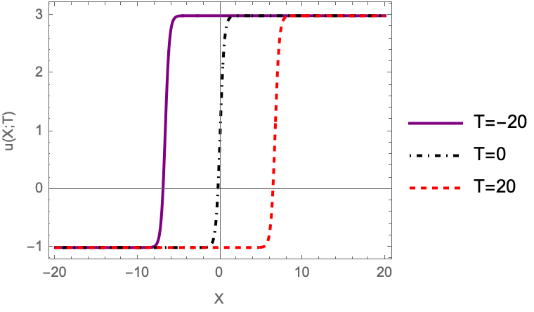
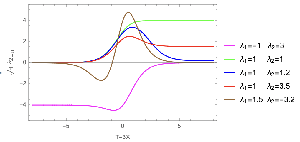
If , solutions to Eq. (3.43) are given by555We should notice here that the -component of the gradient of the single-kink solution is given by hence resembling the shape of the KdV solitary wave. However, one should notice that the amplitude, in this case, is inversely proportional to the velocity of propagation. This implies that taller solitons move slower than shorter ones.
| (3.44) |
Solutions of the form (3.44) represent single-kink which uniformly move left-to-right if or right-to-left if . Notice that the special case returns the constant solution . The parameter determines the position of the kink at , while the parameter characterises, together with the wave speed, its amplitude. Indeed, we have
which implies a global step of amplitude
| (3.45) |
Remark 4.
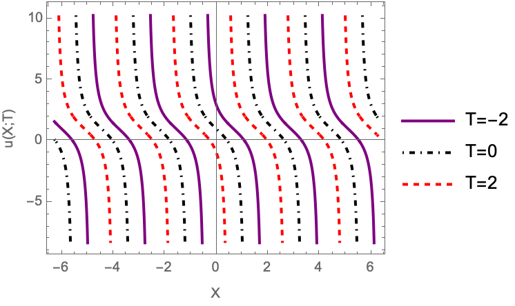
If , by analytic continuation of (3.44), one obtains the periodic singular solutions to Eq. (3.43)
| (3.46) |
Notice that solution (3.46) has infinitely many countable uniformly moving singularities at
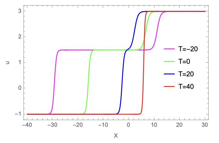
The behaviour of solutions (3.44) and (3.46) is displayed in Figure (1). As expected, the travelling wave profile translates uniformly along the coordinates left-to-right (if ) or right-to-left (if ).
3.2 Travelling wave solutions to Equation (2.28)
Similarly to the analysis carried in Section (3.1), looking for travelling wave solutions to Eq. (2.28) yields
| (3.47) |
which can be straightforwardly integrated to give the following first order ODE for
| (3.48) |
where is an integration constant.
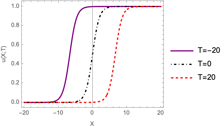
Equation (3.48) resembles the spatially homogeneous reduction of the Kolmogorov–Fisher reaction-diffusion model with logistic growth [28, 29, 30] for fixed linear growth–rate and carrying capacity [3]. Integrating Eq. (3.48), we get the following travelling wave solution
| (3.49) |
where is an integration constant. The value of provides the initial location of the wavefront, meaning the location at which the gradient is maximum (in modulus). Indeed, one notice that and , with also assigning uniquely the asymptotic amplitude of the wave,
Sigmoids (3.49) are displayed in the right panel of Figure (1). Compared to the kink-type solutions obtained for Eq. (2.22), travelling wave solutions for Eq. (2.28) possess a broader transition region connecting the two asymptotic states, and .
4 Multi-kink solutions and shock-particle duality
In Section 3, we have remarked the existence of robust localised travelling wave solutions for Equations (2.22) and (2.28). Equations (3.44) and (3.49) represent indeed kink-type solutions which uniformly translate in both directions, according to the sign of velocity , with respect to the chosen reference frame in Eqs (2.21) and (2.27), respectively. In this Section, we prove the existence of multi-kink solutions for Eqs (2.22) and (2.28), that is solutions relying on the composition of kink–like behavior.
Multi-kink solutions describe fusion and fission of shocks, where in the process no shift in the relative phases of the colliding shocks is observed. When describing shock waves and shock-fitting procedures [31], it is often useful to identify a small parameter which permits to tune the effects of viscous and/or dispersive regularisation mechanisms. For the Bateman-Burgers equation in conservation law form, for instance, a small parameter ahead the viscous term in the current regulates the presence of viscosity and its impact on the solution. In the zero-viscosity limit, the Bateman-Burgers equation turns into the Hopf equation and the behaviour of corresponding solutions drastically changes. When the parameter is kept small but finite, the solutions develop instead classical (viscous) shock waves, displaying regions of high (but finite) gradient whose size can be inferred by the value of the small parameter. Smaller is the parameter, narrower is the region of high gradient of the solution. It is therefore convenient to introduce rescalings of Eq. (1.1) which keep trace of the small positive parameter , consistently with its original derivation. Indeed, in [15], Eq. (1.1) emerged as a viscous conservation law, with the parameter regulating the presence of viscosity. Detaching our analysis from any physical derivation and interpretation of the parameter 666In [15] and other works in the context of statistical thermodynamics, the parameter often arises as the inverse of the number of particles in the statistical ensemble. As a result, performing the zero-viscosity limit o the equation turns to be equivalent to the so-called thermodynamic limit., we will be dealing with two rescalings depending on the value of the quantity .
Case 1: .
In the generic case, , we consider a set of rescaled variables
| (4.50) |
where and are given by (2.21), leading to the following viscous conservation law
| (4.51) |
Case 2: .
In the special case , we can apply a scaling transformation of the form (4.50) to the variables and are given by the transformation (2.27). This brings Eq. (1.1) into the form
| (4.52) |
In the following two subsections we derive and describe multi-kink solutions to Eqs. (4.51) and (4.52) separately.
4.1 Multi-kink solutions to Equation (4.51)
In this Section, we aim to introduce and describe multi-kink solutions to Eq. (4.51) relying on the composition of the kinks obtained in Section 3, where the number of superimposed kinks can be arbitrary. Such solutions are obtained via the application of the Cole-Hopf transformation to an term solution of the equation (2.35), namely
| (4.53) |
where and are real parameters, and
In order to understand the formation of multi-kink solutions, let us observe that the corresponding solution to Eq. (2.28) can be written as follows
| (4.54) |
where we have introduced the weight functions
| (4.55) |
which satisfy the properties
Remark 5.
The decomposition of the solution in terms of weight functions, Eq. (4.54), suggests that the potential function (4.53) can be seen as the partition function associated with a discrete probability distribution (e.g. see [32] and references therein). Following this interpretation, the Cole-Hopf transformation applied to the term function (4.53) gives the (local) average wavenumber. Explicitly, by introducing the statistical free energy , we have . Higher order moments of the distribution can be inferred from higher order derivatives. For instance, the second order moment is given by , or, equivalently, the variance is .
Let for and .777Observe that there might be regions which are empty sets. Therefore, for a given term solution , Eq. (4.53), the plane is a collection of at most distinct non-empty regions . The following proposition holds.
Proposition 1.
In the limit, solutions (4.54) in are approximately given by
Proof.
Let . Dividing numerator and denominator in the r.h.s. of Eq. (4.54) by gives
| (4.56) |
where we have used the fact that in it is for all and, as , we have if . 888Remark that the solution has an essential singularity at and therefore a standard Maclaurin expansion about small and positive is not possible. The statement follows by varying and considering that for all distinct pairs .
Notice that, due to the linearity of functions , regions are bounded by line segments. Such lines emerge as resonance condition of two weight functions, that is
| (4.57) |
and represent the trajectories of classical, viscous, shock waves. In particular, the slope associated with the line is given by and provides the velocity of propagation of the corresponding shock. Resonances between weight functions are in principle allowed and occur at specific points in the -plane. More specifically, the location of the resonance between three adjacent asymptotic states , and is defined by the system of linear equations . Notice that this system admits a unique solution, given that all are distinct and this is so for the shock velocities. Explicitly, by introducing and , the three-term resonance occurs at999Explicitly, we have
| (4.58) |
where the Vandermonde determinant appearing at the denominator is nonzero.
One can also look for higher order resonances, which will eventually lead to points where three or more lines intersect. In general, if the intersection occurs at resonances of weight functions , then solution (4.54) at the intersection point can be approximated by
that is the value of is approximately given by arithmetic mean of the corresponding asymptotic states. It is also worth to stress that the for a given term function , the plane is a collection of at most distinct regions . Formula (1) can be seen as the asymptotic solution in the regime of small viscosity and is actually a time-dependent generalised Heaviside step function.
Remark 6.
The scheme adopted above to characterise the multi-kink behaviour has been to design a skeleton in the space of independent variables corresponding to different asymptotic values of the dependent variable. The resulting approximation in the limit, Eq. (4.56), could be also equivalently seen as the tropical limit of the term solution (4.54) (see e.g. [33, 34] and Refs. therein). Indeed, more standardly, one may perform the approximation at the level of the potential function (4.53), resulting into The application of the Cole-Hopf transformation to the approximated potential function would still give in .
The decomposition of the solution (4.53) in terms of elementary single-kink solutions, can be understood as follows. Let and be two adjacent regions characterised by parameters , and , , respectively. In the region , we have that
| (4.59) |
where we have used the fact that for it is and for all , and as we have and . The approximation in Eq. (4.59) is just the single-kink solution found in Eq. (3.44), upon identifying the kink speed with and integration constants as
| (4.60) |
Remark 7.
4.1.1 Shock–particle duality
Before analysing the shock dynamics, we should first identify the mass and momentum associated with the conservation law. Let be the momentum density at time and location . The total momentum at a given time is given by
| (4.61) |
where and , with , are precisely the asymptotic values of the solution at that time , that is
In Eq. (4.61), we have used the fact that for at any time . Let be the mass density. The total mass at time is given by
Notice that total mass, momentum and velocity are consistently related through the relation , where is the velocity of a shock between the most outer states, . Remarkably, mass and momentum are conserved quantities for this system, that is (the prime meaning now the -derivative), and conservations of mass and momentum emerge as for a scattering process. More explicitly, we have
| (4.62) | ||||
| (4.63) |
where ‘in’ and ‘out’ label mass and velocities of the shocks before and after scattering101010A subtle remark is needed here. Actually, one retrieves scattering among classical (point-like) particles in the limit , that is when mass and momentum are strongly localised about the centre of each shock. For small but finite, and outside the interaction region, one can simply identify the mass and momentum carried by each shock by performing an integral over a domain of size of order centred about the shock location. , respectively, and the summation is performed over all pairs of wavenumbers involved in the scattering. In Eqs. (4.62)-(4.63), we have identified the mass and the momentum carried by each individual shock as and . Conservation of mass is nonetheless the analogous of Rankine-Hugoniot jump condition for a fluid supporting discontinuous shock waves [31]. From this point of view, the equation of interest (1.1), or (4.51), represents viscous regularisation [25] of the continuity equation by the flow density
where here . This procedure is different from the usual Burgers regularisation, , when and , or dispersive ones (see e.g. [35] and references therein). We will discuss in detail the shock dynamics, including the conservation laws (4.62) and (4.63), with the aid of some examples.
We first start with the case of terms in Eq. (4.53). This case represents indeed the elementary fusion or fission of shocks, as displayed in Figure 2 where a relatively large value of has been chosen to magnify the finite-size region of high gradient. The Left panel shows the fission process of a shock wave entering at with velocity and mass decaying in two shocks of velocities and masses equal to , and , , respectively. The Right panel exhibits instead the – transformed solution representing two shocks of velocities and masses equal to , and , merging into a single shock with mass and velocity and , respectively. Notice that asymptotic states in the Right panel take the values , and . The location and time of collision for the processes (highlighted with black circles) are computed by formula (4.58) giving and , respectively. Semi-lines of resonance , and , defined by Eq. (4.57), emerge from the dashed and dash–dotted lines simply obtained in both processes as conditions for all pairs of indices .
Fusion and fission processes are reversible due to the –like symmetry enjoyed by Eq. (4.51). For instance, the fusion process of two shocks in the right panel is obtained by application of the transformation defined in Eq. (2.17) to the solution representing the fission of two shocks displayed in the left panel. The resulting processes resemble those of the fission of a particle of mass into two particles of masses and , and the fusion of two particles of masses and to give a particle of mass , respectively.

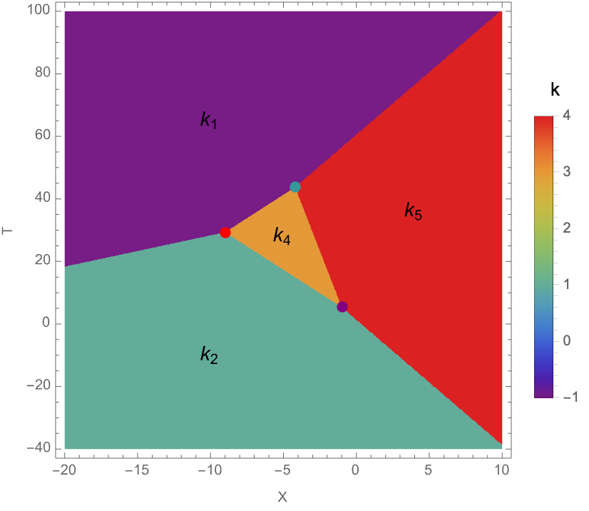
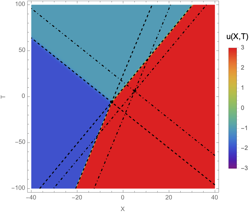
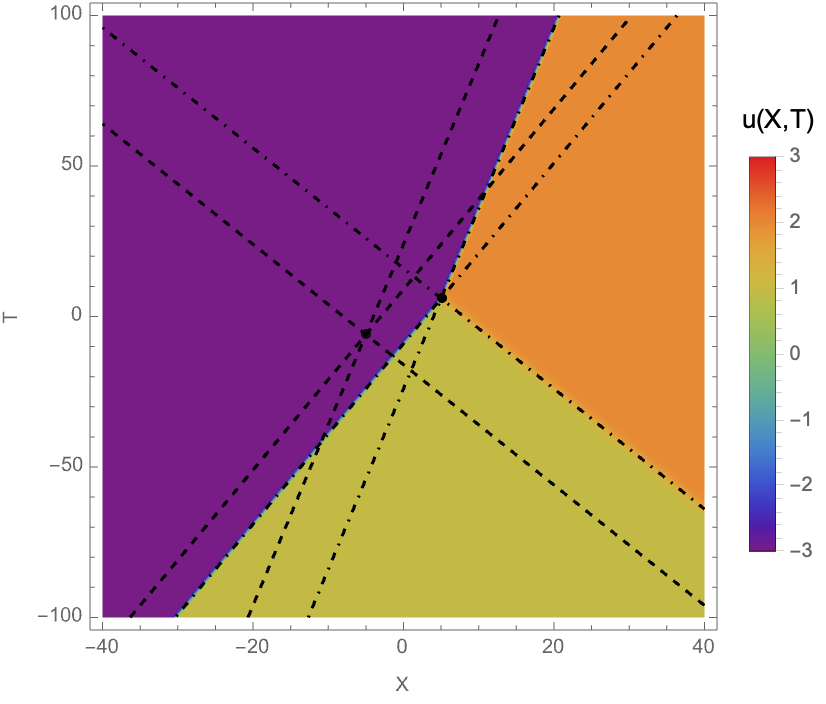
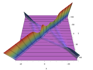
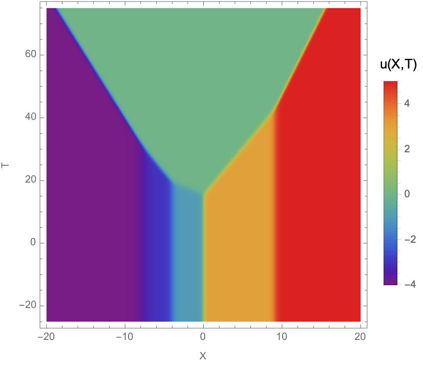
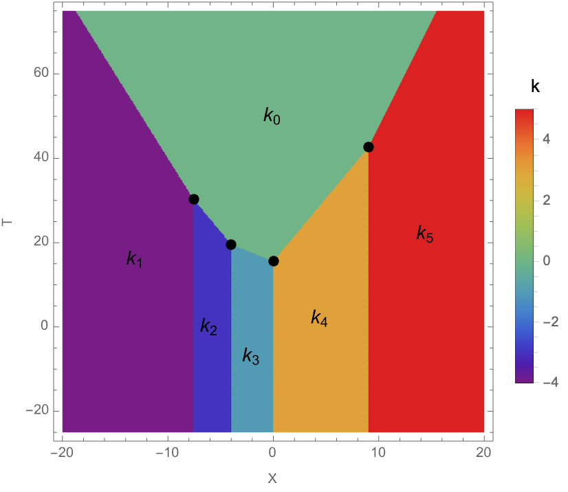
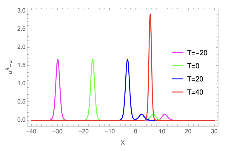
Let us now analyse Figure 3, which was obtained from terms in Eq. (4.53). On the right, our geometric construction, which we refer as asymptotic solution, displays four different regions , , and characterised by wavenumber , , and separated by six line segments: , , , , and . The corresponding multi-kink solution for is displayed to the left, showing agreement with the geometric construction. Each line segment correspond to the trajectory of a kink, thought as a classical viscous shock wave. Shock fission, i.e. generation of multiple kinks from a single one, occurs when two lines originate from one. Shock confluence or fusion occurs instead when two shocks collide to form a single shock. The dynamics of shocks can be understood in terms of inelastic scattering, that is particle-particle collisions where new particles are formed from old ones while preserving the overall mass and momentum. Shock fission can be understood as a particle decay. Similarly, confluence of shocks is understood as fusion of particles. Conservation of mass and momentum are therefore expressed in terms of conservation of mass and momentum of shocks. Direct application of conservation laws (4.62)-(4.63) to the case of a fission of one shock to form a pair of shocks gives
| (4.64) | ||||
| (4.65) |
Eqs. (4.64) and (4.65) can be straightforwardly generalised to other shock fusion/fission processes. Relatively to the example under study, the shock between the regions and , which is approximately in amplitude (or mass), performs a fission to two shocks: one, to the left, having amplitude and another one, to the right, having amplitude . Therefore the mass of the incoming shock is distributed across the two outgoing shocks such that mass is conserved in the scattering process. The same happens for momentum. In fact, from (4.61) one deduces for any value of , given that the asymptotic states at are the same at all times.
Asymptotically, the overall process can be described as a fission of two shocks with three intermediate shocks enclosing a transient state (). In this example, shocks interact forming a network of shaped trajectories [36]. Two fissions and one fusion are displayed at and , respectively.
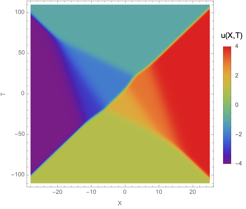
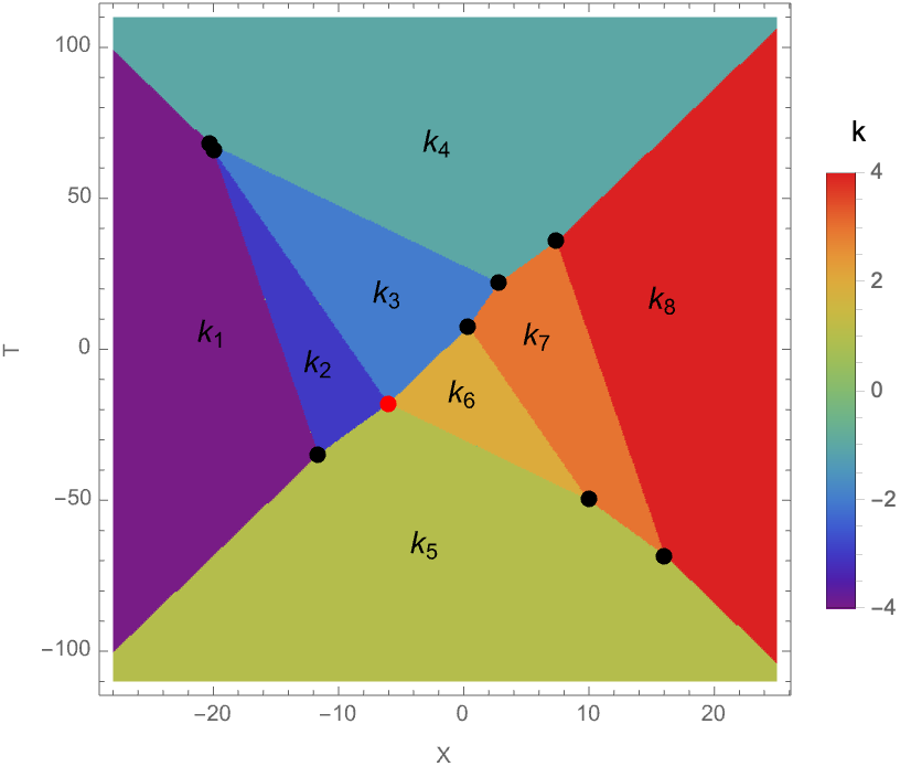
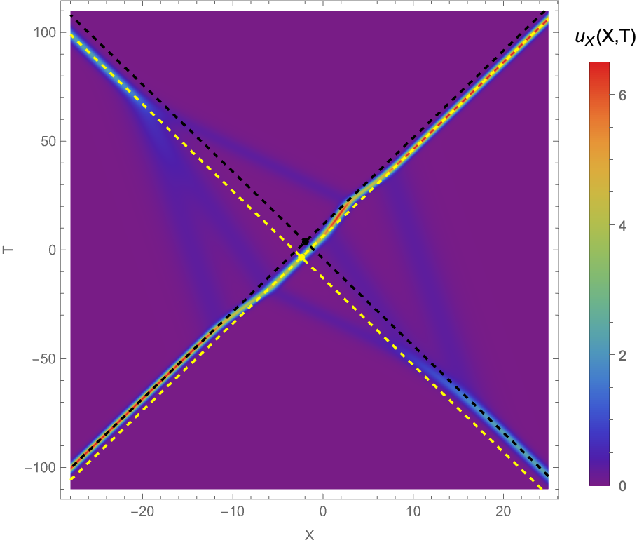
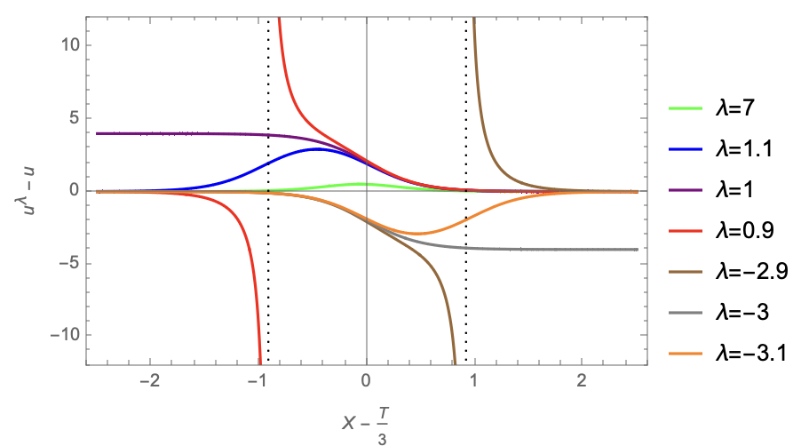
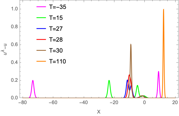
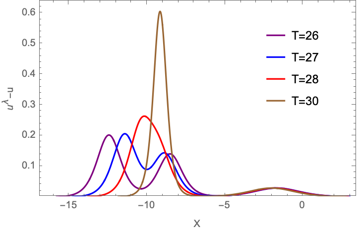
A more complex scenario emerges in Fig (4), where an example of a term solution is considered. The overall process results in a scattering between two initial shocks of mass and momentum , and , , respectively, to give two final shocks of mass and momentum , and , . However, four metastable states, labelled with , , and , appear. Remarkably, the two shocks between states and , and and collide at to form two new shocks between states and , and and (red circle in Fig (4)). Notice that mass and momentum are conserved through the collision. It is also important to remark that the asymptotic states, that is the solution at large positive and negative times, could be described by two colliding particles, one moving from left to right with mass and velocity , and another one with mass and velocity . The effect of the collision results in an effective phase-shift, that is the two initial particles are either delayed or advanced compared to the case of non-interacting particles. Indeed, extending the trajectories of the four asymptotic shocks to the central, transient region, one notices that the trajectories do not intersect in a single point. This situation can be better analysed by looking at the behaviour of , as displayed in Fig (5). The two set of lines are indeed parallel in pairs, meaning that the velocities of the ingoing and outgoing shocks are the same. However, the fact that lines do not coincide suggests the presence of an effective phase shift. In fact, the intersection points, thought as the centres of the scattering in the linear interaction regime, are given by and , respectively. The phase-shift of both shock waves produces a shift in position, , which is given by a Galilean transformation with , where subscripts ‘’ and ‘’ label the shocks propagating left-to-right and right-to-left, respectively. Away from the interaction, shocks travel with uniform rectilinear motion as they were free particles. Indeed, one can notice that the interaction between the incoming shocks start to occur at about and seems to be negligible for . For , that is for , an interesting dynamics emerge, where multiple intermediate shocks are formed, traced by peaks in the gradient. Notice that higher is the peak, larger is the mass transported by the shock.
4.2 Multikink solution for Equation (4.52)
The arguments leading to the derivation and analysis of multi-kink solutions of Eq. (4.52) slightly differ from those concerning Eq. (4.51). Indeed, the general solution (2.30) poses a severe limitation on the structures that can be employed while conceiving solutions displaying kinks. In practice, (2.30) and its counterpart with rescaled variables, Eq. (4.52), is compatible with the presence of a nonlinear superposition of terms in the form , where, differently from Eq. (4.51), terms with the null-momentum are allowed and obey to a distinct dispersion relation. Without loss of generality, let and for . Multi-kink solutions to Eq. (4.52) take the form
| (4.66) |
with and for . Similarly to the case , we can identify domains in which are dominant, that is for and . Regions are bounded by line segments which are now of two types depending on the wavenumbers characterising the two adjacent states. More precisely, the line segments
identify trajectories of viscous shocks, which are either stationary, that is with velocity , if , or move with velocity if . Similarly to solutions to Eq. (4.51), the following proposition is implied.
Proposition 2.
In the limit , solutions (4.66) in are approximately given by
Proof.
The proof is obtained by introducing weight functions and is identical to that in Proposition 1.
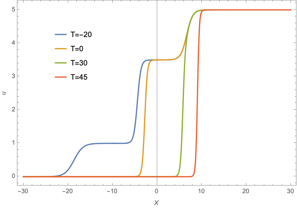
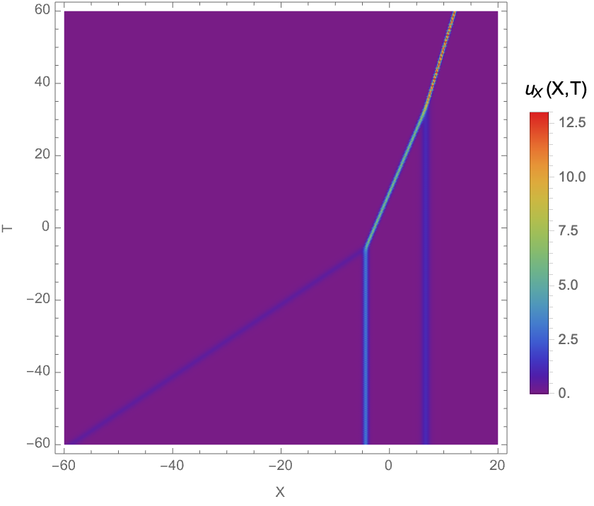
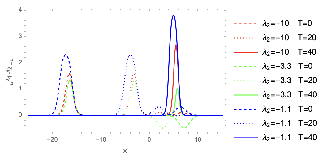
Plots can be given to illustrate the implied dynamics at different times, see for instance Figures 6 and 7. Figure 7 shows that the solution is initially, for , approximately stationary111111Notice that, solution (4.66) can be written in the form (2.30) with and . As a result, the time dependence is visible only when the term is sufficiently large compared to terms . , displaying four shocks at rest. When a first fission occurs at , generating an inner vacuum state and two shocks travelling in opposite directions. Multiple fusions occur until only two shocks survive at large times, i.e. . One can verify that, similarly to the case , introducing the mass and momentum densities, and , respectively, total mass and momentum are conserved. Explicitly, we have
| (4.67) | ||||
| (4.68) |
where labels the outer states at as before. This holds also locally at each shock fission/fusion process. Analogously to Eqs. (4.64) and (4.65), conservation of mass and momentum in an elementary fusion of two shocks takes the simple form
| (4.69) | ||||
| (4.70) |
For instance, Figure 6 displays the multiple fusions of a shock of amplitude (or mass) travelling with velocity with two stationary shocks of amplitude and . In the first collision, a shock of amplitude is produced, which moves with velocity , hence fulfilling conservation of mass and momentum.
5 Bäcklund Transformations for Equation (2.22)
Bäcklund transfomations (BTs) remodel a given nonlinear PDE into some other PDE, thereby relating the solutions of the two [37]. This strategy has proved highly beneficial to generate answers to nonlinear PDEs, playing a fundamental role in the growth of activities and interest in soliton theory. BTs generally link two functions in a system of first order PDEs, the two functions being a BT if they both satisfy the PDE independently. In this Section we deal with problem of finding Bäcklund transformations for the Equation (2.22).
5.1 One–parameter Bäcklund transformations
In this Subsection, we set up BTs for the Equation (2.22). Aimed at this, we employ a strategy that is similar to that developed for determining BTs in the case of the Bateman-Burgers equation. That is, let us turn back to the linear equation (2.35) pertinent to Equation (2.22) and consider a special solution . Then, the corresponding solution for is given by (2.31), i.e. . Now, also the function satisfies the equation (2.35). Therefore, a new solution will be given by
| (5.71) |
Since , by combining the previous relations, one can eliminate the auxiliary function to obtain the formula
| (5.72) |
as in the Bateman-Burgers case. This is a very special case of Bäcklund transformation, allowing us to generate a new solution for Eq. (2.22) from a known one. Formula (5.72) may have, however, a limited use as far as one is interested in smooth functions. For example, it leads immediately to a singular class of solutions for the case of travelling waves (3.44) in Figure 1. A possible ‘way out’ stands in striving to put forward a generalisation of the above line of reasoning by imposing the dependency on an auxiliary parameter. The objective is to bring in a control parameter able to rule out singular solutions if not germane to the phenomenology aforethought for the very specific problem dealt with (1.1). In particular, we can proceed with this idea by introducing a parameter according to
| (5.73) |
as it can be proved by direct substitution of into Eq. (2.22).
Remark 4.
It is noteworthy that when we formulate the problem (2.22) in the form (2.25), the corresponding Bäcklund transformation reads
| (5.74) |
This result can be proved by direct substitution of the expressions (5.74) into the system (2.25). Then, by using the same system to simplify the coefficients of , one can verify that they are correctly posed.
To make a plain instance of the outcomes from (5.73), and of the functioning of the introduced auxiliary parameter, we can apply this transformation to the travelling wave solution (3.44), so to get
| (5.75) |
The BT puts into effect the introduction of another travelling component adding to the initial profile of and moving with the same velocity, determined by the r.h.s. of (5.75). Singularities occur if .
Figure 8 shows the variety of results for Eq. (5.75) while varying the parameter . The solution to which the BT (5.73) is applied is the same considered in the first panel of Figure 1, namely Eq. (3.44) with , and . The Left panel in Figure (8) shows the generation and removal of singularities occurring for such new shape component while tuning the auxiliary parameter , along with the deformations of logistic sigmoids generating equal asymptotic limits and flattening the generated extremum. For and , for instance, the solution is regular in the whole domain. When singularities originate (brown and red curves).
For positive (resp. negative) close to the value (resp. ) bumps develop as displayed in the blue curve (resp. orange), but as long as the value of is taken sufficiently far away from the range , curves flatten about the horizontal axis, as displayed by the green curve. The right panel provides examples of the motion for the additional travelling component that adds to via BT to define the solution .
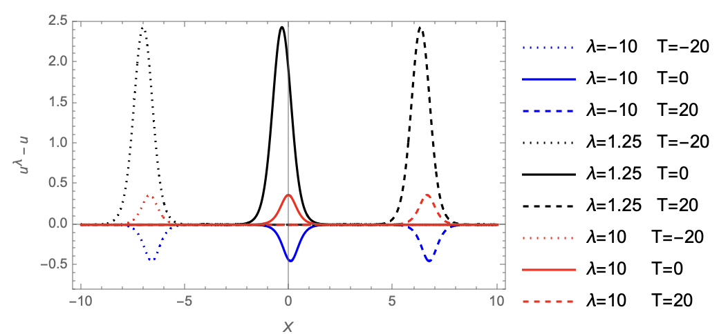
We can also provide other examples of solutions obtained by application of (5.73) by resorting to the kink-type solution (4.54) that we derived earlier in Section 4. Notice that singularities for (5.73) are prevented provided that . The plot on the left of Figure 9 shows the evolution of a solution (4.54) with . The solution exhibits, at successive values of , fusions that absorb the intermediate plateau while progressing towards the direction of increasing values. The second plot discloses the differences at the same values of between and . Two initial travelling components approach each other, their location being centred about the high-gradient regions and their magnitude being larger when a higher gradient is required to connect two asymptotic states. The two components ultimately merge, originating a peaked profile moving according to the latest fusion process. Higher values of introduce more articulated shapes and interactions, of course. Nevertheless, essential features are preserved for the overall dynamics. This is supported by Figure (10), showing the dissimilarities between and are when in the case . A pronounced peak forms for the function at large (orange curve in the left plot), after a cascade of interactions between the different travelling components. The interaction occurring for times is better evidenced by the close-up in the right panel.
5.2 Two–parameter Bäcklund transformations
Having obtained BTs in the form (5.73) and understood the effects of their auxiliary parameter , we can now go further and analyse the action of BTs involving two parameters by suitable composition of single parameter BTs. Indeed, owing to the Cole-Hopf transform (2.31) and its derivative w.r.t. , one obtains a generalisation of (5.71), namely
| (5.76) |
and the linear combination is a new solution of the linear problem (2.35). This suggests to take two distinct values of the transformation parameter, say and , and use the above relation (5.73) to provide the solutions and , which actually coincide. Moreover, eliminating the explicit presence of the parameters, one can find a superposition formula like
| (5.77) |
In terms of the function one obtains the formula
| (5.78) |
The BTs established above can be exploited repeatedly and combined to originate further solutions. For instance, a Bianchi permutability scheme can be superimposed as follows. One can start by combining two BTs generated by the same seed solution in correspondence of two different parameters. The application of a second BT with the interchanged parameters, and further, the request of compatibility of the results, leads to a formula which provides a fourth solution in the form of an algebraic (nonlinear) expression of the previous three ones.
We now compare results from the implementation of one- and two-parameter BTs. Let the seed function be once again the travelling wave (3.44). The application of formula (5.77) yields
| (5.79) |
where
| (5.80) |
Figure 11 shows examples of effects from the application of a two-parameter BT (5.77) for different values of and . Potential roots of the denominator are displayed at
| (5.81) |
However, in Figure 11 we have avoided to take into account singular cases.
Effects on the travelling wave solution (1) have been delved into first. The consists of fixed profiles travelling. Depending on the values of and , extrema can be generated and asymptotes can be affected (Left panel). The application of formula (5.77) in respect to the solution for in Eq. (4.66) is shown in the Right panel. Our findings validate arguments parallel to those inferred while referring to the action of a BT (5.75) on the same multi-kink solution.
6 Conclusions and future perspectives
The present communication has been devoted to the study of the nonlinear non-evolutive PDE (1.1), which can be seen as a generalised Fokker-Planck equation encoding a density-dependent diffusivity, and nontrivial nonlinearity and viscous effects. The equation, which was introduced in [15] for the description of real gases within a mean-field framework, is potentially applicable to general circumstances where a conservation law is foreseen with a current that depends (linearly) also on first derivative of both spatial- and time-type local variables, in fact.
A first measure in our analysis has been to identify two sets of coordinates through the implementation of two distinct linear transformations on the dependent and independent variables, i.e. Eqs. (2.14) and (2.27). Such transformations allows us to make the analysis of the resulting PDEs independent on the structural parameters of the model equation under study, provided that a discerning constraint is assessed ( or ). This clearly led to a simplification of the differential problem and a more favourable starting point for the analysis of its integrability features.
We worked out a concrete study with reference to travelling wave solutions and presented a comprehensive clarification of dynamics for a class of naturally discerned multi-kink solutions, that incidentally turned out to be characterised by a simple reciprocal dispersion relation. By first restoring the role of the small parameter originally associated with viscosity in the conservation law (1.1), we provide an interpretation of multi-kink solutions, in the limit , in terms of classical viscous shock waves. Our analysis and description of multi-kink solutions relies on a scheme that entails the partitioning of the space of independent variables into disjoint regions where each of the exponential terms contributing to the sum is dominant (see Eq. (4.53)). The small viscosity regime of the multi-kink solution results into approximating the sum with the dominant term in each region and is analogous to the so-called tropical limit (see Eq. (4.56)) [33, 38, 39]. The lines which separate the disjoint regions constitute the fundamental information about shock trajectories and their interaction, their intersections providing the collision location and time (see explicit formula (4.58)). We identified conserved quantities, such as mass and momentum, for the differential equations under study in the two different cases and analyse d the interaction between shocks as scattering processes among particles. This allowed us to establish a shock–particle duality, which was detailed with the aid of representative examples. In particular, we showed that conservation of mass and momentum for the underlying equations can be formulated as analogous conservation laws for particles (see Eqs. (4.62) and (4.63)). We also proved that, sufficiently far from the interaction, the multi-kink solution is approximated as a collection of travelling waves in the form of single kinks, like those determined in Section 3, hence demonstrating that there is no phase-shift resulting from the kink-kink interaction.
Our understanding of integrability features of Eq. (1.1) has been later enhanced by the devising of Bäcklund transformations (BTs) depending on auxiliary parameters, whose effect has been argued showing the generation of travelling components adding to the shape of the naked solution. To achieve this, we have discussed examples of the applications of one- and two- parameter BTs.
Our analysis has introduced new useful insights into solutions and properties of Equation (1.1). Nonetheless, several lines of investigation can be yet pursued related to its solvability and integrability. These comprise the existence and analysis of solutions subject to other relevant (dynamical or boundary) conditions. Among others, special solutions which can be written in terms of theta functions may be sought, following the procedures employed for the Bateman-Burgers [40] or other PDEs (see e.g. [41, 42] and Refs. therein). Other fundamental directions can also be explored, such as those arising from our findings in the context of the Hirota method, BTs and Lax pairs. For instance, the implementation of the Hirota method accounting for the improvements related to the introduction of combinatorial methods [43, 44] may be assessed. Moreover, a systematic study of higher order (generalized) symmetries [8, 9] is also missing. By all such methods one may be led to retrieve novel classes of solutions (maybe made of distinct interacting components as in [45]), design different Bäcklund transformations, seek for insights concerning a Lax pair formulation and identify infinitely many commuting conservation laws for the nonlinear PDE (1.1). Yet another direction of study can be the discretisation of the model and the subsequent queries raised and application of devoted tools, e.g. the Inverse Spectral Transform following the guidance developed in [16]. Last but not least, extensions to higher dimensions of (1.1) could be constructed. Beyond presumably offering a richer phenomenology and new classes of solutions, as usually it happens in nonlinear soliton equations in higher dimensions (see e.g. [46] and Refs. therein), these might either establish or strengthen the connection with known and widely studied higher dimensional models, e.g. reductions from Navier-Stokes equations other than the Bateman-Burgers one, higher order Fisher or Fokker-Planck equations and so forth [13, 47, 48, 28].
Finally, we wish to highlight insights and perspectives offered by our study in the originating context of Eq. (1.1). Indeed, the integrability structure of the model discussed in this work shares similarities with a plethora of one- and multi-component models recently studied in the realm of statistical physics (see for instance [49, 50, 32] to cite a few). One of the key–features of all those models is the fact that order parameters, as functions of thermodynamic variables, fulfil nonlinear C-integrable conservation laws of viscous type. The C-integrability property implies that the partition function of the model obeys to a linear differential identity, playing incidentally the role of a linearising potential function linked to the order parameter through a Cole-Hopf transformation. As a result, the partition function is a sum of exponential terms of the form , with the parameter , being the number of particles in the statistical ensemble. In that context, each function is full determined by the energy and statistical weight of each allowed macrostate of the system. The results presented in this work imply that the thermodynamic limit for models with a countable number of macrostates could be seen as a tropical limit, hence establishing links with the work [51], where the Authors shed light on the relevance of the tropical limit in statistical physics, intended as the limit , with being the Boltzmann constant. We feel that our approach and results may lead to advancements in the asymptotics of order parameters for a large class of C-integrable models and potentially describe statistical systems exhibiting complex cascades of phase transitions.
Acknowledgments
FG and GL would like to thank the Isaac Newton Institute for Mathematical Sciences, Cambridge, for support and hospitality during the programmes “Dispersive Hydrodynamics: mathematics, simulation and experiments, with applications in nonlinear waves” and “Emergent phenomena in nonlinear dispersive waves” where work on this paper was undertaken. This work was supported by EPSRC grant no EP/R014604/1. FG also acknowledges the hospitality of the Lecce’s division of INFN and of the Department of Mathematics and Physics ’Ennio De Giorgi’ of the University of Salento. GL and LM acknowledge the hospitality of the School of Mathematics and Statistics of the University of Glasgow. INFN IS-MMNLP partially supports GL and LM. GL is also partially supported by INFN IS-GAST. Authors are indebted to C Gilson, Y Kodama, B Konopelchenko and A Moro for useful discussions and remarks.
Competing interests
The author(s) has/have no competing interests to declare.
Licence
For the purpose of open access, the authors have applied a Creative Commons Attribution (CC BY) licence to any Author Accepted Manuscript version arising from this submission.
References
- [1] see e.g.: T.D: Bennett, Transport by Advection and Diffusion, Wiley, New York, 2013.
- [2] see e.g.: Y. Epshteyn, C. Liu and M. Mizuno, A stochastic model of grain boundary dynamics: a Fokker- Planck perspective, Math. Models Methods Appl. Sci. 32, 2189-236 (2022), and Refs. therein.
- [3] see e.g.: J.D. Murray, Mathematical Biology, Springer-Verlag, New York, 2013.
- [4] see e.g.: G. Furioli, A. Pulvirenti, E. Terraneo and G. Toscani, Fokker–Planck equations in the modeling of socio-economic phenomena, Math. Mod. Meth. Appl. Scie. 27, 115-158 (2017), and Refs. therein.
- [5] R. J. Field and M. Burger (Eds.), Oscillations and Traveling Waves in Chemical Systems, Wiley, Chichester, 1985.
- [6] See e.g.: T.D. Frank, Nonlinear Fokker-Planck Equations. Fundamentals and Applications, Springer Series in Synergetics, Springer, Berlin, 2010, and Refs. therein.
- [7] F. Giglio, G. Landolfi and A. Moro, Integrable extended van der Waals model, Physica D333, 293-300 (2016).
- [8] I.S. Krasilshchik and A.M. Vinogradov (Eds.), Symmetries and Conservation Laws for Differential Equations of Mathematical Physics, Translation of Mathematical Monographs series, AMS, Providence, 1999.
- [9] P. Olver, Applications of Lie Groups to Differential Equations Graduate Texts in Mathematics, 107, Springer-Verlag, New York, 1993.
- [10] V.V. Sokolov, On the symmetries of evolution equations, Russ. Math. Surv. 43, 165-204 (1988).
- [11] A.A. Abramenko, V.I. Lagno and A.M. Samoilenko, Group Classification of Nonlinear Evolutionary Equations: II. Invariance Under Solvable Groups of Local Transformations, Differ. Equ. 38, 502-509 (2002).
- [12] V.I. Lagno and A.M. Samoilenko, Group classification of nonlinear evolution equations. I. Invariance under semisimple local transformation groups, Differ. Equ. 38, 384–391 (2002).
- [13] T. Benjamin, J. Bona and J. Mahony, Models equations for long waves in nonlinear dispersive systems, Philos. Trans. R. Soc. Lond. Ser. A272, 47-78 (1972).
- [14] F. Giglio, G. Landolfi. L. Martina and A. Moro, Symmetries and criticality of generalised van der Waals models, J. Phys. A: Math. Theor. 54, 405701 (2021).
- [15] F. Giglio, G. Landolfi and L. Martina, On solutions to a novel non-evolutionary integrable 1 + 1 PDE, J. Phys. A: Math. Theor. 56, 485205 (2023).
- [16] D. Levi, O. Ragnisco and M. Bruschi, Continuous and discrete matrix Burgers’ hierarchies, Nuovo Cim. 74, 33–51 (1983).
- [17] R. Hirota, The Direct Method in Soliton Theory, Cambridge University Press, Reading, 2004 (Trans. from Japanese by C. Gilson, A. Nagai and J. Nimmo).
- [18] J. Hietarinta, Introduction to the Hirota bilinear method, In: Y. Kosmann-Schwarzbach, B. Grammaticos, and K.M. Tamizhmani (Eds), Integrability of Nonlinear Systems. Lecture Notes in Physics, 495, Springer, Berlin, 1997.
- [19] P.J. Olver, Evolution equations possessing infinitely many symmetries, J. Math. Phys. 18, 1212-1215 (1977).
- [20] T. Kahawara, The derivative-expansion method and nonlinear dispersive waves, J. Phys. Soc. Jpn. 35, 1537-1544 (1973).
- [21] A. Jeffrey and T. Kahawara, Asymptotic methods in Nonlinear Wave Theory, Pitman Books Ltd, London, 1982.
- [22] A. H. Nayfeh, Perturbation Methods, Wiley, New York, 2000.
- [23] C.M. Bender and S.A. Orszag, Advanced Mathematical Methods for Scientists and Engineers, Springer, New York (1999).
- [24] R.E. O’Malley, The Method of Matched Asymptotic Expansions and Its Generalizations, in: R.E. O’Malley (Ed.) Historical Developments in Singular Perturbations, Springer, Cham, 2014.
- [25] A. Arsie, P. Lorenzoni and A. Moro, Integrable viscous conservation laws, Nonlinearity 28, 1859-1895 (2015).
- [26] E. Cartan, Oeuvres complètes, Vol. 2, Editions CNRS, Paris, 1984.
- [27] M.J. Ablowitz and H. Segur, Solitons and the Inverse Scattering Transform, SIAM, Philadelphia, 1981.
- [28] Y. Du and W. Ni, The High Dimensional Fisher-KPP Nonlocal Diffusion Equation with Free Boundary and Radial Symmetry, SIAM J. Math. Anal. 54, 3930-3973 (2022).
- [29] R. A. Fisher, The Wave of Advance of Advantageous Genes, Ann. Eugenics 7, 353-369 (1937).
- [30] P. Grindrod, The theory and applications of reaction-diffusion equations: Patterns and waves, Oxford Applied Mathematics and Computing Science Series, The Clarendon Press Oxford University Press, New York, 1996.
- [31] G. B. Whitham, Linear and Nonlinear Waves, Wiley, New York, 1974; Chapt. 4.
- [32] G. De Matteis, F. Giglio and A. Moro, Complete integrability and equilibrium thermodynamics of biaxial nematic systems with discrete orientational degrees of freedom, Proc. R. Soc. A. 480, 20230701 (2024).
- [33] T. Kato, Dynamical Scale Transform in Tropical Geometry, World Scientific, New Jersey, 2016.
- [34] C. Athorne, D. Maclagan and I. Strachan (Eds.), Tropical Geometry and Integrable Systems, Contemporary Mathematics, 580, AMS, 2012.
- [35] G.A. El, M.A. Hoefer and M. Shearer, Dispersive and Diffusive-Dispersive Shock Waves for Nonconvex Conservation Laws, SIAM Rev. 59, 3-61 (2017).
- [36] Y. Kodama, KP Solitons and the Grassmannians. Combinatorics and Geometry of Two-Dimensional Wave Patterns, Springer Briefs in Mathematical Physics, 22, Springer, Singapore (2017).
- [37] see e.g.: C. Rogers and W.K. Schief, Bäcklund and Darboux transformations, Cambridge University Press, Cambridge, 2002, and Refs. therein.
- [38] Y. Kodama and L. Williams, Combinatorics of KP Solitons from the Real Grassmannian, in: A.B. Buan, I. Reiten and Ø. Solberg (Eds.), Algebras, Quivers and Representations: The Abel Symposium 2011, Springer, Heidelberg, 2013; pp. 155-193.
- [39] A. Dimakis and F. Müller-Hoissen, KdV soliton interactions: a tropical view, J. Phys. Conf. Ser. 482, 012010 (2014).
- [40] A. Parker, On the periodic solution of the Burgers equation: a unified approach, Proc. R. Soc. A438, 113-132 (1992).
- [41] M. Bertola, R. Jenkins and A. Tovbis, Partial degeneration of finite gap solutions to the Korteweg-de Vries equation: Soliton gas and scattering on elliptic backgrounds, Nonlinearity 36, 3622 (2023).
- [42] Y. Kodama, KP solitons and the Riemann theta functions, Lett. Math. Phys. 114, 41 (2024).
- [43] C. Gilson, F. Lambert, J. Nimmo and R. Willox, On the combinatorics of the Hirota D-operators, Proc. R. Soc. Lond. A45, 2223-234 (1996).
- [44] W-X. Ma, Bilinear equations, Bell polynomials and linear superposition principle, J. Phys.: Conf. Ser. 411, 012021 (2013).
- [45] Y. Zarmi, Soliton-generating -functions revisited, J. Math. Phys. 59, 122701 (2018).
- [46] B.G. Konopelchenko, Solitons In Multidimensions: Inverse Spectral Transform Method, World Scientific, Singapore, 1993.
- [47] S. Wang, X. Tang, and S. Lou, Soliton fission and fusion: Burgers equation and Sharma–Tasso–Olver equation, Chaos, Solitons Fractals 21, 231–239 (2004).
- [48] P.F. Han and T. Bao, Dynamical behavior of multiwave interaction solutions for the (3+1)-dimensional Kadomtsev-Petviashvili-Bogoyavlensky-Konopelchenko equation, Nonlinear Dyn. 111, 4753-4768 (2023).
- [49] A. Moro, Shock dynamics of phase diagrams, Ann. of Phys. 343 , 49-60 (2014).
- [50] G. Biondini, A. Moro, B. Prinari and O. Senkevich, -star models, mean-field random networks, and the heat hierarchy, Phys. Rev. E105, 014306 (2022).
- [51] M. Angelelli and B. Konopelchenko, Tropical Limit in Statistical Physics, Phys. Lett. A379, 1497-1502 (2015).