A more novel approach of radiative linear seesaw in a modular symmetry
Abstract
We propose a radiatively induced linear seesaw model that is perfectly realized at leading order by a modular symmetry. Because this group also has a flavor symmetry, we obtain some predictions concentrating on two specific regions at nearby fixed points and . Through our numerical chi square analysis, we show predictions for each the case depending on the neutrino mass ordering; normal and inverted one.
I Introduction
Understanding the neutrino mass structure is one of our important tasks beyond the standard model(BSM). Although a renown model would be a canonical seesaw mechanism Yanagida (1979); Minkowski (1977); Mohapatra and Senjanovic (1980); Zee (1980) introducing heavy right-handed neutral fermions, it would be difficult to test this model since it demands much higher energy scale than the current experimental energy scale, i.e. TeV. Linear seesaw mechanism Wyler and Wolfenstein (1983); Akhmedov et al. (1996a, b) is well-known as providing a verifiable model in current experiments at TeV scale introducing left-handed and right-handed neutral fermions 111An inverse seesaw mechanism also requests these neutral fermions and leads to a similar motivation of linear seesaw Wyler and Wolfenstein (1983); Mohapatra and Valle (1986).. In basis of , the mass matrix of neutral fermions to realize the linear seesaw is given by
| (4) |
Assuming the following mass hierarchies
| (5) |
we find the following active neutrino mass matrix
| (6) |
In a view point of model building, most of models put the condition, especially , in Eq. (5) by hand. There exit some ways to realize this condition. Below, we review two examples. The first example is to introduce multiplet particles (larger than triplet) that have nonzero vacuum expectation value (VEV) and generate via this VEV after the spontaneous symmetry breaking. Since this VEV receives a constraint GeV from electroweak precision test, would be realized when is obtained via VEV of the SM Higgs. In ref. Nomura and Okada (2019a), is obtained via VEV of quartet Higgs boson. Also hidden Abelian gauge symmetry is introduced in order to realize the mass matrix in Eq (4). The second example is to generate at loop level by introducing new particles. In ref. Das et al. (2017), is induced at one-loop level in which singly-charged heavier leptons and two types of singly-charged bosons run. In addition, an Abelian gauge symmetry and discrete symmetry are introduced to realize the model.
In this paper, we construct a one-loop induced linear seesaw mechanism revisiting our previous paper Das et al. (2017). In fact, this paper has unsatisfactory point; it includes an inverse seesaw mechanism as a leading order as well as linear seesaw. Therefore, we could not completely control the desired mass matrix in Eq. (4) via introduced two additional symmetries. In order to resolve this defect, we introduce a modular symmetry. Surprisingly, this symmetry solely realizes linear seesaw mechanism and gives us predictions at nearby the fixed points in both cases of neutrino mass hierarchies. 222There exists wide variety of applications to explain lepton and quark masses and mixings as well as new physics Feruglio (2019); Criado and Feruglio (2018); Kobayashi et al. (2018); Okada and Tanimoto (2019); Nomura and Okada (2019b); Okada and Tanimoto (2021a); de Anda et al. (2020); Novichkov et al. (2019); Nomura and Okada (2021); Okada and Orikasa (2019); Ding et al. (2019a); Nomura et al. (2020); Kobayashi et al. (2019); Asaka et al. (2020a); Zhang (2020); Ding et al. (2019b); Kobayashi et al. (2020); Nomura et al. (2021); Wang (2020); Okada and Shoji (2020); Okada and Tanimoto (2023); Behera et al. (2022a, b); Nomura and Okada (2022, 2020); Asaka et al. (2020b); Okada and Tanimoto (2021b); Nagao and Okada (2022); Okada and Tanimoto (2021c); Kang et al. (2022); Ding et al. (2024); Ding and King (2023); Nomura et al. (2024a); Kobayashi et al. (2024); Petcov and Tanimoto (2024); Kobayashi and Tanimoto (2023); Nomura and Okada (2024a); Qu and Ding (2024); Nomura and Okada (2024b); Nomura et al. (2024b). Through our numerical chi square analysis, we demonstrate several predictions later.
This paper is organized as follows. In Sec. II, we review our setup of the modular assignments introducing new particles and explain how to realize our scenario by showing the charged-fermion sector and the neutral fermion sector. In Sec. III, we demonstrate chi-square numerical analyses concentrating on two fixed points and show what kinds of predictions we obtain. Finally, we summarize and conclude in Sec. IV.
II Model setup
In this section we show the model. The particle contents are almost the same as the model in ref. Das et al. (2017) where we remove one scalar singlet. Then new filed contents are neutral singlet fermions and , charged singlet fermions and , inert doublet scalar and inert charged scalar . For symmetry of the model, we removed from the original model and added modular one. The field contents and charge assignments of them are summarized in Table 1. Under these symmetries, the renormalizable Lagrangian is given by
| (7) |
where is a trivial singlet abbreviating free parameters that are explicitly demonstrated later.
, , , and are modular couplings that are uniquely fixed when modulus is determined Feruglio (2019). In our paper, we concentrate on specific region at nearby fixed points .
Renormalizable Higgs potential is found as
| (8) |
where is a second Pauli matrix and several free parameters include modular forms in mass and non-dimensional parameters.
II.1 Charged-lepton mass matrix
The mass matrix of charged-lepton comes from the first term in Eq. (7) after spontaneous electroweak symmetry breaking and it is found as
| (15) |
where can be real parameters without loss of generality. is diagonalized by . Therefore, where diag.. From , are fixed to fit the three observed charged-lepton masses.
| (16) | |||
| (17) | |||
| (18) |
therefore combinations can be rewritten in terms of three charged-lepton mass eigenvalues and as follows:
| (19) | |||
| (20) | |||
| (21) |
It suggests that are obtained as a result of solution of the following equation:
| (22) |
Then, the tadpole condition; , gives the following solutions
| (23) |
Since all solutions have to be positive reals and Eq. (23) simply increases, we need the following conditions:
| (24) |
where (i1,2,3) corresponds to , depending on hierarchies among these parameters. These conditions are helpful to have our numerical analysis.
II.2 Heavier charged-lepton mass matrix
The mass matrix of heavier charged-lepton comes from the term in Eq. (7) as follows:
| (28) |
where can be real parameters without loss of generality while the others are complex values. is diagonalized by . Therefore, . Flavor eigenstate are written in terms of mass eigenstate and their mixing matrix as follows: .
II.3 Neutral fermion mass matrix
The mass matrix of neutral fermions comes from the following terms after spontaneous electroweak symmetry breaking;
| (29) |
In basis of , the neutral fermion mass matrix is given by
| (33) |
where each of mass matrix is given by
| (40) | ||||
| (44) | ||||
| (48) |
is given at one-loop level through the second line in Eq. (7) as follows:
| (49) | ||||
| (50) | ||||
| (57) | ||||
| (61) |
Since is induced at one-loop level, we can naturally suppose to be the minimum mass scale among these mass matrices. is proportional to that is the electroweak scale GeV, while and are directly generated by the bare mass Lagrangian. Therefore we expect and scale to be 1 TeV that originates from our expected new physics beyond the SM. Moreover, we have a non-unitary condition that comes from several experimental constraints related to electroweak observables such as the SM W boson mass , the effective Weinberg angle, several ratios of Z boson fermionic decays, invisible decay of Z, electroweak universality, measured CKM, and lepton flavor violations. Therefore is required both experimentally and theoretically. Hence, the following mass ordering is naturally realized:
| (62) |
Under these mass hierarchies, the active neutrino mass matrix at leading order is given by 333Although we have the inverse seesaw mass matrix , this term is next leading order due to the hierarchies in Eq. (62).
| (63) |
The overall mass parameter is determined by the atmospheric neutrino mass-squared difference and dimensionless neutrino mass eigenvalues:
| (64) |
where NH and IH respectively stand for the normal and inverted hierarchies. The dimensionless mass eigenvalues for the active neutrinos are obtained by diagonalizing the mass matrix as , therefore . Then the observed mixing matrix is defined by . Subsequently, the solar neutrino mass-squared difference is fixed to be
| (65) |
has to be within the allowed range of the experimental value, in NuFit 5.2 Esteban et al. (2020). The sum of neutrino mass eigenvalues is given by
| (66) |
is constrained by the minimal standard cosmological model 120 meV by CDM Vagnozzi et al. (2017); Aghanim et al. (2020). However, it is weaker if the data is analyzed in the context of extended cosmological models Olive et al. (2014). Moreover, DESI and CMB data combination recently provides more stringent upper bound on the sum as 72 meV Adame et al. (2024). The effective mass for neutrinoless double beta decay is given by
| (67) |
where are mixing of , are Majorana phases, and is Dirac CP phase. is constrained by the current KamLAND-Zen data measured in future Abe et al. (2024), and the current upper bound is given by meV at 90 % confidence level. Here the range of the bound is due to the use of different method in estimating nuclear matrix elements.
III Numerical analysis and phenomenology
In this section we show chi square analysis to fit the neutrino oscillation data where we refer to NuFit 5.2 Esteban et al. (2020) as we mentioned in the last section, and Dirac CP phase as well as Majorana phase are considered as an output predictions since any values are allowed by experiments at 3 confidence level (C.L.). Therefore, we make the use of five reliable observables []. Moreover, we focus on the region at nearby two fixed points and . We randomly select our input parameters in the ranges of for dimensionless values and for mass dimension ones respectively where we take the mass input parameters so that the non-unitarity condition is satisfied as discussed in the subsection II.3.
III.1 NH
Here we summarize our findings for NH case.
III.1.1
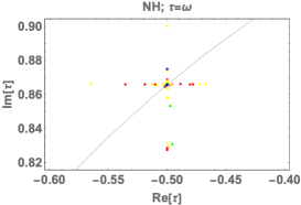
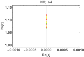
Here, we start to discuss the case of in NH. In Fig. 1, we show allowed region of Re[] and Im[] at nearby . The blue, green, yellow and red points represent the parameter sets that respectively satisfy the range of , , , and C.L. estimated by chi square analysis, where the black solid line is boundary of the fundamental domain at . One finds there is deviation only when or .
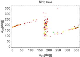
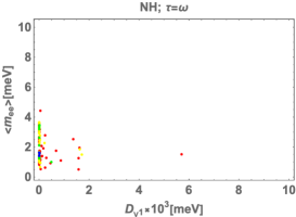
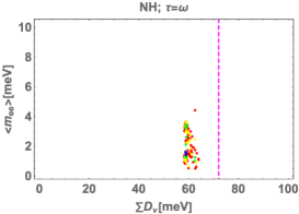
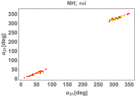
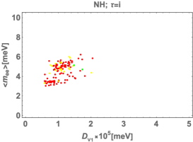
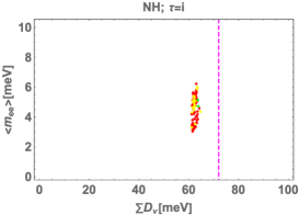
In Fig. 2, we show some allowed regions of Majorana phases (left), in terms of the lightest neutrino mass eigenvalue (center), and in terms of (right). All the color legends are the same as the one in Fig. 1. The dotted pink vertical line in the right figure shows the upper limit from the combination of the DESI and CMB data that is meV. In the left figure, we find is allowed by the ranges []. Although is allowed by whole the ranges, there is a unique correlation between these two Majorana phases. For example, tends to be localized at nearby and except this region Majorana phases are uniquely fixed if either of them is determined. In the center figure, we found [meV] and [meV] both of which are too tiny to test by experiments where the most of the points are localized at nearby meV. In the right figure, we found [meV] that could be testable in a cosmological experiments/observations such as DESI and CMB data combination in near future.
III.1.2
In Fig. 3, we show allowed region of Re[] and Im[] at nearby . All the color legends are the same as the one of Fig. 1. Allowed range is .
In Fig. 4, we show some allowed regions of Majorana phases (left), in terms of the lightest neutrino mass eigenvalue (center), and in terms of (right). All the color legends are the same as the one of Fig. 2. In the left figure, we find there are two localized islands; , and . Moreover, Majorana phases are uniquely fixed if either of them is determined due to simple correlation. In the center figure, we found [meV] and [meV] both of which are so tiny to test by experiments. In the right figure, we found [meV] that could be testable in a cosmological experiments/observations such as DESI and CMB data combination near future.
III.2 IH
Here we summarize our findings for IH case.
III.2.1
In Fig. 5, we show allowed region of Re[] and Im[] at nearby in case of IH. All the color legends are the same as the one in Fig. 1. We find that the allowed region is uniformly located around the fixed point.
In Fig. 6, we show some allowed regions of Majorana phases (left), in terms of the lightest neutrino mass eigenvalue (center), and in terms of (right). In the center figure, the horizontal dotted gray line is the lower bound 36 meV. In the right one, the red vertical line is the cosmological upper bound 120 meV. All the other legends are the same as the one of Fig. 2. In the left figure, we find there are two localized islands; , and . In the center figure, we found [meV] and [meV]. Even though the lightest neutrino mass is too tiny, is localized at nearby the lower bound on 36 meV that would be tested near future. In the right figure, we found [meV] that could also be testable by cosmological observations.
III.2.2
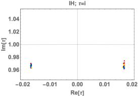
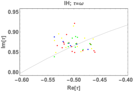
In Fig. 7, we show allowed region of Re[] and Im[] at nearby in case of IH. All the color legends are the same as the one of Fig. 1. We find that the allowed region is localized in two small islands.
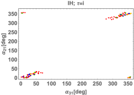
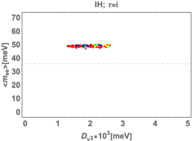
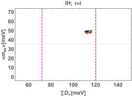
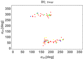
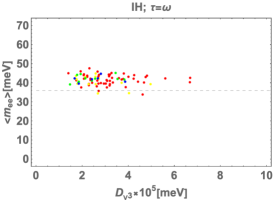
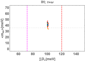
In Figs. 8, we show some allowed regions of Majorana phases (left), in terms of the lightest neutrino mass eigenvalue (center), and in terms of (right). In the center figure, the horizontal dotted gray line is the lower bound 36 meV. In the right one, the red vertical line is the cosmological upper bound 120 meV. All the other legends are the same as the one of Fig. 2. In the left figure, we find there are two larger localized islands; , and , and two smaller localized islands; , and . In the center figure, we found [meV] and [meV]. Although the lightest neutrino mass is too tiny, is close to the lower bound on 36 meV that would be tested near future. In the right figure, we found [meV] that is close to the cosmological upper bound and it could also be testable near future
IV Summary and discussion
We have proposed a radiatively induced linear seesaw model perfectly controlling the desired neutral fermion mass matrix at the leading order through a modular flavor symmetry. The nature of the symmetry provides a crucial improvement of our previous model in ref. Das et al. (2017) reducing assumptions to realize linear seesaw mechanism. Furthermore, thanks to this modular symmetry, we have obtained some predictions of neutrino observables focusing on specific regions at nearby two fixed points and . In the following, we remark several features in our findings.
Even though the case of has allowed points almost on , there is deviation from a little for both the cases of NH and IH. In case of and with NH, can be testable in a cosmological experiments/observations in near future although the other mass observables are too tiny. In case of and with IH, and can be testable in current experiments near future.
Acknowledgments
The work was supported by the Fundamental Research Funds for the Central Universities (T. N.).
References
- Yanagida (1979) T. Yanagida, Phys. Rev. D 20, 2986 (1979).
- Minkowski (1977) P. Minkowski, Phys. Lett. B 67, 421 (1977).
- Mohapatra and Senjanovic (1980) R. N. Mohapatra and G. Senjanovic, Phys. Rev. Lett. 44, 912 (1980).
- Zee (1980) A. Zee, Phys. Lett. B 93, 389 (1980), [Erratum: Phys.Lett.B 95, 461 (1980)].
- Wyler and Wolfenstein (1983) D. Wyler and L. Wolfenstein, Nucl. Phys. B 218, 205 (1983).
- Akhmedov et al. (1996a) E. K. Akhmedov, M. Lindner, E. Schnapka, and J. W. F. Valle, Phys. Lett. B 368, 270 (1996a), eprint hep-ph/9507275.
- Akhmedov et al. (1996b) E. K. Akhmedov, M. Lindner, E. Schnapka, and J. W. F. Valle, Phys. Rev. D 53, 2752 (1996b), eprint hep-ph/9509255.
- Mohapatra and Valle (1986) R. N. Mohapatra and J. W. F. Valle, Phys. Rev. D 34, 1642 (1986).
- Nomura and Okada (2019a) T. Nomura and H. Okada, Phys. Rev. D 99, 055033 (2019a), eprint 1806.07182.
- Das et al. (2017) A. Das, T. Nomura, H. Okada, and S. Roy, Phys. Rev. D 96, 075001 (2017), eprint 1704.02078.
- Feruglio (2019) F. Feruglio, Are neutrino masses modular forms? (2019), pp. 227–266, eprint 1706.08749.
- Criado and Feruglio (2018) J. C. Criado and F. Feruglio, SciPost Phys. 5, 042 (2018), eprint 1807.01125.
- Kobayashi et al. (2018) T. Kobayashi, N. Omoto, Y. Shimizu, K. Takagi, M. Tanimoto, and T. H. Tatsuishi, JHEP 11, 196 (2018), eprint 1808.03012.
- Okada and Tanimoto (2019) H. Okada and M. Tanimoto, Phys. Lett. B 791, 54 (2019), eprint 1812.09677.
- Nomura and Okada (2019b) T. Nomura and H. Okada, Phys. Lett. B 797, 134799 (2019b), eprint 1904.03937.
- Okada and Tanimoto (2021a) H. Okada and M. Tanimoto, Eur. Phys. J. C 81, 52 (2021a), eprint 1905.13421.
- de Anda et al. (2020) F. J. de Anda, S. F. King, and E. Perdomo, Phys. Rev. D 101, 015028 (2020), eprint 1812.05620.
- Novichkov et al. (2019) P. Novichkov, S. Petcov, and M. Tanimoto, Phys. Lett. B 793, 247 (2019), eprint 1812.11289.
- Nomura and Okada (2021) T. Nomura and H. Okada, Nucl. Phys. B 966, 115372 (2021), eprint 1906.03927.
- Okada and Orikasa (2019) H. Okada and Y. Orikasa (2019), eprint 1907.13520.
- Ding et al. (2019a) G.-J. Ding, S. F. King, and X.-G. Liu, JHEP 09, 074 (2019a), eprint 1907.11714.
- Nomura et al. (2020) T. Nomura, H. Okada, and O. Popov, Phys. Lett. B 803, 135294 (2020), eprint 1908.07457.
- Kobayashi et al. (2019) T. Kobayashi, Y. Shimizu, K. Takagi, M. Tanimoto, and T. H. Tatsuishi, Phys. Rev. D 100, 115045 (2019), [Erratum: Phys.Rev.D 101, 039904 (2020)], eprint 1909.05139.
- Asaka et al. (2020a) T. Asaka, Y. Heo, T. H. Tatsuishi, and T. Yoshida, JHEP 01, 144 (2020a), eprint 1909.06520.
- Zhang (2020) D. Zhang, Nucl. Phys. B 952, 114935 (2020), eprint 1910.07869.
- Ding et al. (2019b) G.-J. Ding, S. F. King, X.-G. Liu, and J.-N. Lu, JHEP 12, 030 (2019b), eprint 1910.03460.
- Kobayashi et al. (2020) T. Kobayashi, T. Nomura, and T. Shimomura, Phys. Rev. D 102, 035019 (2020), eprint 1912.00637.
- Nomura et al. (2021) T. Nomura, H. Okada, and S. Patra, Nucl. Phys. B 967, 115395 (2021), eprint 1912.00379.
- Wang (2020) X. Wang, Nucl. Phys. B 957, 115105 (2020), eprint 1912.13284.
- Okada and Shoji (2020) H. Okada and Y. Shoji, Nucl. Phys. B 961, 115216 (2020), eprint 2003.13219.
- Okada and Tanimoto (2023) H. Okada and M. Tanimoto, Phys. Dark Univ. 40, 101204 (2023), eprint 2005.00775.
- Behera et al. (2022a) M. K. Behera, S. Singirala, S. Mishra, and R. Mohanta, J. Phys. G 49, 035002 (2022a), eprint 2009.01806.
- Behera et al. (2022b) M. K. Behera, S. Mishra, S. Singirala, and R. Mohanta, Phys. Dark Univ. 36, 101027 (2022b), eprint 2007.00545.
- Nomura and Okada (2022) T. Nomura and H. Okada, JCAP 09, 049 (2022), eprint 2007.04801.
- Nomura and Okada (2020) T. Nomura and H. Okada (2020), eprint 2007.15459.
- Asaka et al. (2020b) T. Asaka, Y. Heo, and T. Yoshida, Phys. Lett. B 811, 135956 (2020b), eprint 2009.12120.
- Okada and Tanimoto (2021b) H. Okada and M. Tanimoto, Phys. Rev. D 103, 015005 (2021b), eprint 2009.14242.
- Nagao and Okada (2022) K. I. Nagao and H. Okada, Nucl. Phys. B 980, 115841 (2022), eprint 2010.03348.
- Okada and Tanimoto (2021c) H. Okada and M. Tanimoto, JHEP 03, 010 (2021c), eprint 2012.01688.
- Kang et al. (2022) D. W. Kang, J. Kim, T. Nomura, and H. Okada, JHEP 07, 050 (2022), eprint 2205.08269.
- Ding et al. (2024) G.-J. Ding, S.-Y. Jiang, S. F. King, J.-N. Lu, and B.-Y. Qu (2024), eprint 2404.06520.
- Ding and King (2023) G.-J. Ding and S. F. King (2023), eprint 2311.09282.
- Nomura et al. (2024a) T. Nomura, H. Okada, and H. Otsuka, Nucl. Phys. B 1004, 116579 (2024a), eprint 2309.13921.
- Kobayashi et al. (2024) T. Kobayashi, T. Nomura, H. Okada, and H. Otsuka, JHEP 01, 121 (2024), eprint 2310.10091.
- Petcov and Tanimoto (2024) S. T. Petcov and M. Tanimoto (2024), eprint 2404.00858.
- Kobayashi and Tanimoto (2023) T. Kobayashi and M. Tanimoto (2023), eprint 2307.03384.
- Nomura and Okada (2024a) T. Nomura and H. Okada (2024a), eprint 2407.13167.
- Qu and Ding (2024) B.-Y. Qu and G.-J. Ding (2024), eprint 2406.02527.
- Nomura and Okada (2024b) T. Nomura and H. Okada (2024b), eprint 2409.10912.
- Nomura et al. (2024b) T. Nomura, H. Okada, and O. Popov (2024b), eprint 2409.12547.
- Esteban et al. (2020) I. Esteban, M. C. Gonzalez-Garcia, M. Maltoni, T. Schwetz, and A. Zhou, JHEP 09, 178 (2020), eprint 2007.14792.
- Vagnozzi et al. (2017) S. Vagnozzi, E. Giusarma, O. Mena, K. Freese, M. Gerbino, S. Ho, and M. Lattanzi, Phys. Rev. D 96, 123503 (2017), eprint 1701.08172.
- Aghanim et al. (2020) N. Aghanim et al. (Planck), Astron. Astrophys. 641, A6 (2020), [Erratum: Astron.Astrophys. 652, C4 (2021)], eprint 1807.06209.
- Olive et al. (2014) K. A. Olive et al. (Particle Data Group), Chin. Phys. C 38, 090001 (2014).
- Adame et al. (2024) A. G. Adame et al. (DESI) (2024), eprint 2404.03002.
- Abe et al. (2024) S. Abe et al. (KamLAND-Zen) (2024), eprint 2406.11438.