Optimized Homomorphic Vector Permutation From New Decomposition Techniques

Abstract

Homomorphic permutations are fundamental to privacy-preserving computations based on word-wise homomorphic encryptions, which can be accelerated through permutation decomposition. This paper defines an ideal performance of any decomposition on permutations and designs algorithms to achieve this bound.

We start by proposing an algorithm searching depth-1 ideal decomposition solutions for permutations. This allows us to ascertain the full-depth ideal decomposability of two types of permutations used in specific homomorphic matrix transposition (SIGSAC 18) and multiplication (CCSW 22), enabling these algorithms to achieve asymptotic improvement in speed and rotation key reduction.

We further devise a new strategy for homomorphically computing arbitrary permutations, aiming to approximate the performance limits of ideal decomposition, as permutations with weak structures are unlikely to be ideally factorized. Our design deviates from the conventional scope of permutation decomposition and surpasses state-of-the-art techniques (EUROCRYPT 12, CRYPTO 14) with a speed-up of up to $\times 2.27$ under the minimum requirement of rotation keys.

1 Introduction

Homomorphic encryption (HE) is a powerful cryptographic primitive that supports computations on encrypted data, enabling secure cross-domain data processing. Currently, the prevailing RLWE (ring learning with error) based HE schemes utilizing batch encoding [1, 2, 3] supports constructing various privacy-preserving computation tasks. The methodology can be summarized as follows: we use basic homomorphic operations (e.g., addition, multiplication) to build modules like homomorphic matrix operations [4, 5, 6] and function evaluations [7, 8, 9, 10], which are further combined and arranged to form complete computation tasks such as neural network training and inference [11, 12].

Since ciphertexts carry plaintext vectors (which can be further seen as matrices) in the batch-encoding HE setting, the homomorphic permutation [13, 4] of components within the plaintext vector becomes a critical bridge connecting fundamental operations and upper modules. Notably, the implementation of homomorphic permutation requires meticulous consideration, and its complexity tends to dominate in modules like matrix operations.

Specifically, homomorphic permutation typically involves ciphertext rotation and plaintext-ciphertext multiplication: the former allows for the cyclic shifting of the plaintext vector within the ciphertext, while the latter is responsible for selecting the components to be shifted (masking by multiplying binary vectors). Ciphertext rotation, however, involves time-consuming number-theoretic transforms (NTT) over the polynomial ring, which are the most computationally intensive operations in RLWE-based homomorphic encryption. Moreover, ciphertext rotation for different shift steps requires different rotation keys, which must be generated by the private key holder and can be as large as several ciphertexts. A large number of rotation keys imposes significant overhead on both communication and storage. These characteristics make the performance of homomorphic permutation crucial when constructing higher-level homomorphic operation modules. Previous optimization methods for homomorphic permutation can be roughly divided into the following categories:

• The first category involves deconstructing ciphertext rotations and rearranging the execution sequence of their subroutines to reduce the computational overhead for the entire set of rotation. This includes the hoisting technique proposed by Halevi et al.[5] and its extended version (termed double-hoisting) introduced by Bossuat et al.[9]

• The second category decomposes a single permutation into composite permutations, each of which requires fewer entry rotations, thereby reducing the number of homomorphic automorphisms and/or the evaluation keys. This includes using the Benes network to construct efficient circuits for arbitrary permutation proposed by Gentry et al.[13, 4] The idea of decomposition is later applied to specific linear transformations[14, 15] to reduce time and space complexity.

For the second type of optimization, We believe that it has not yet been thoroughly explored. In this paper, we demonstrate that, whether for specific permutations or arbitrary ones, there are decomposition methods that yield more effective optimizations.

1.1 Technique Overview & Contributions

We first analyze the possible optimal improvements that decomposition can bring to homomorphic permutations and define an ideal form of decomposition (Section 2.3). Broadly speaking, this definition demands that for each additional multiplication depth, the total rotation scale of the permutation should be approximately halved. Currently, no algorithm guarantees such a level of decomposition for arbitrary permutations.

Starting from Section 3, we propose decomposition methods that achieve (or better approximate) the ideal optimization effect for specific and general permutations. Our concrete contribution can be listed as follows:

(i) We design an algorithm to find an (approximate) solution for depth-1 ideal decomposition, which tries to factorize a permutation matrix $U$ into $U_{L}U_{R}+E$ where the number of non-zero diagonal elements in $U_{R}$ and $E$ remains constant and the number of non-zero diagonal elements in $U_{L}$ is half that of $U$.

(ii) With the assistance of contribution (i), we discover the full-depth ideal decomposability of a specific permutation used in homomorphic matrix transposition (HMT) by Jiang et al.[6] and elucidate its equivalence to sequential and recursive block-wise operations on the matrix to be transposed. This decomposition pattern also proves useful in the homomorphic matrix multiplication (HMM) proposed by Rizomiliotis and Triakosia[16], where we introduce further modifications to reduce the total decomposition depth cost to a constant 1 and enhance the utilization of encoding space.

(iii) Not every permutation guarantees an ideal decomposability. Therefore, we propose a novel method to compute arbitrary homomorphic permutations, offering a new approach to approximate the ideal performance. Roughly speaking, we construct a multi-group network structure where its nodes take vectors as input and output, applying rotations with varying steps. Through precise node transmission logic and tailored homomorphic operations, our approach outperforms the state-of-the-art implementation using the Benes network [13, 4] under minimal rotation key requirements.

2 Background and Prelimary

2.1 Notations

We denote scalars and polynomials by lowercase letters, vectors by bold lowercase letters, and matrices by uppercase letters. $A[i,j]$ represents the element in the $i$th row and $j$th column of matrix $A$. The diagonal index of $A$ equals the column index of the first element in the $0$th row of that diagonal. We use $A(k,l)_{r}$ to indicate the element located in the $l$th row on the $k$th diagonal of $A$, and $A(k,l)_{c}$ to denote the element situated in the $l$th column on the $k$th diagonal of $A$. These three coordinate representations can be converted as follows:

$$\begin{split}A(k,l)_{r}=A[l,k+l],\quad&A[i,j]=A(j-i,i)_{r}\\ A(k,l)_{c}=A[l-k,l],\quad&A[i,j]=A(j-i,j)_{c}\\ A(k,l)_{r}=A(k,k+l)_{c},\quad&A(k,l)_{c}=A(k,l-k)_{r}\end{split}$$ (1)

2.2 Batch-encoding Homomorphic Encryption

The so-called batch-encoding homomorphic encryption is a class of HE schemes based on the security assumption of RLWE [17, 18], which supports vector spaces as plaintext spaces [1, 13, 2, 3]. These schemes typically enable homomorphic coordinate-wise operations.

Typically, for a vector $\mathbf{z}$ to be encrypted, a batch-encoding HE scheme first maps it onto some polynomial ring space $R=\mathbb{Z}[X]/(X^{N}+1)$ with $N$ a power of $2$. The mapped plaintext polynomial, denoted $pt(\mathbf{z})$, is then encrypted into a ciphertext $ct(\mathbf{z})$ in $R_{Q_{\ell}}^{2}=(\mathbb{Z}_{Q_{\ell}}[X]/(X^{N}+1))^{2}$ where $Q_{\ell}=\prod_{i=0}^{\ell}q_{i},0\leq\ell<L$ for some pre-determined modulus chain $[q_{0},\dots,q_{L-1}]$. Such ciphertext generally supports the following homomorphic operations:

• $\texttt{Add}(ct(\mathbf{z}_{1}),ct(\mathbf{z}_{2}))$: For the input ciphertexts $ct(\mathbf{z}_{1})\in R_{Q_{\ell}}^{2}$ and $ct(\mathbf{z}_{2})\in R_{Q_{\ell^{\prime}}}^{2}$, output $ct(\mathbf{z}_{1})+ct(\mathbf{z}_{2})\bmod{Q_{\min(\ell,\ell^{\prime})}}$, which is a valid ciphertext of $\mathbf{z}_{1}\oplus\mathbf{z}_{2}$.

• $\texttt{CMult}(ct(\mathbf{z}_{1}),pt(\mathbf{z}_{2}))$: For the input ciphertext $ct(\mathbf{z}_{1})\in R_{Q_{\ell}}^{2}$ and plaintext $pt(\mathbf{z}_{2})\in R_{Q_{\ell^{\prime}}}$, output $ct(\mathbf{z}_{1})\cdot pt(\mathbf{z}_{2})\bmod{Q_{\min(\ell,\ell^{\prime})}}$ as a valid ciphertext of $\mathbf{z}_{1}\otimes\mathbf{z}_{2}$.

• $\texttt{Mult}(ct(\mathbf{z}_{1}),ct(\mathbf{z}_{2}),rlk)$: For the input ciphertexts $ct(\mathbf{z}_{1})\in R_{Q_{\ell}}^{2}$ and $ct(\mathbf{z}_{2})\in R_{Q_{\ell^{\prime}}}^{2}$, compute the tensor product $ct(\mathbf{z}_{1})\cdot ct(\mathbf{z}_{2})\bmod{Q_{\min(\ell,\ell^{\prime})}}$ in $R_{Q_{\min(\ell,\ell^{\prime})}}^{3}$. Using the relinearization key $rlk$, switch it back to $R_{Q_{\min(\ell,\ell^{\prime})}}^{2}$ and output it as a valid ciphertext of $\mathbf{z}_{1}\otimes\mathbf{z}_{2}$.

• $\texttt{Rescale}(ct)$: For the input ciphertext $ct\in R_{Q_{\ell}}^{2}$, Rescale reduces the scaling factor of the underlying plaintext by $\frac{Q_{\ell}}{Q_{\ell-1}}$, resulting in the output: $\lfloor\frac{Q_{\ell}}{Q_{\ell-1}}\cdot ct\rceil\bmod{Q_{\ell-1}}\in R_{Q_{\ell-1}}^{2}$. This operation is necessary when processing the output of a Mult or CMult, as the scaling factor of the plaintext in such ciphertexts grows exponentially.

• $\texttt{Rot}(ct(\mathbf{z}),k)$: For the input ciphertext $ct(\mathbf{z})$, apply the Galois automorphism corresponding to $k$, cyclically shifting each component of the underlying vector $\mathbf{z}$ by $k$ positions (to the left if $k$ is positive, otherwise to the right). Then, apply the implicit input rotation key $rtk_{k}$ to ensure that the decryption remains consistent with the private key.

From the above routines, we summarize some common constraints of batch-encoding homomorphic encryption schemes:

1. Batch-encoding HE only natively supports homomorphic operations with a limited multiplication depth of $L-1$, as $Q_{L}$ provides at most $L-1$ moduli to support Rescale operations.

2. The complexity order of the routines is: $\texttt{Mult}\approx\texttt{Rot}>\texttt{Rescale}>\texttt{CMult}>\texttt{Add}$. This is because all polynomial multiplications and additions are performed in the NTT (Number Theoretic Transform) domain, with an asymptotic complexity of $O(N)$, while fraction multiplications and base decompositions involved in Mult and Rot require switches in and out of the NTT domain with a complexity of $O(N\log{N})$.

3. A rotation key consists of multiple ciphertexts obtained by encrypting some Galois automorphism of $s$ after decomposing it in some base and multiplying by the modulus chain $P$. A Large number of rotation keys may cause a great burden on key generation and a high communication overhead for transmitting the keys. This can be a significant factor affecting system efficiency in some multi-party scenarios.

2.3 Homomorphic Permutation

Given a ciphertext $ct(\mathbf{x})$ encrypting an $n$-dimensional plaintext vector $\mathbf{x}$ and a length-$n$ permutation $p$ to be applied to $\mathbf{x}$, the homomorphic permutation $ct(p(\mathbf{x}))$ can be represented as a homomorphic linear transformation (HLT) $ct(U\mathbf{x})$, where $U$ is the matrix representation of $p$, and $\mathbf{u}_{i}$ denotes the vector comprising all elements along the $i$-th diagonal of $U$. The expression $ct(U\mathbf{x})$ can be computed via the following BSGS (Baby-Step Giant-Step) equation (with $n=n_{1}n_{2}$):

$$\begin{split}\sum_{i=0}^{n_{2}-1}\texttt{Rot}\left(\sum_{j=0}^{n_{1}-1}\left(\mathbf{u}_{i,j}\odot\texttt{Rot}(ct(\mathbf{x});j)\right);n_{1}\cdot i\right).\end{split}$$ (2)

where $\mathbf{u}_{i,j}=\texttt{Rot}(\mathbf{u}_{n_{1}\cdot i+j};-n_{1}\cdot i)$.

If there exists a common difference $a$ and range $d\leq\lfloor n/a\rfloor$ such that non-zero diagonals are distributed over an arithmetic sequence $s=\{a\cdot i\mid 0\leq i\leq d\}$, a slight modification of BSGS yields a rotation complexity of $O(d_{1}+d_{2})$ with $d_{1}d_{2}=d$ the new inner and outer loop counts. Hoisting techniques proposed by Halevi et al. and Bossuat et al. provide the BSGS algorithm with a trade-off between speed and the number of rotation keys required. Broadly, this requires $O(d_{1}+d_{2})$ rotation keys and enables the speed of HLT to increase with the BSGS ratio $d_{1}/d_{2}$ within a certain range (potentially $1\sim 16$).

2.3.1 Optimization Through Decomposition

Equations 2 imply that the complexity of homomorphic permutation implemented by HLT is closely related to the number of non-zero diagonals in matrix $U$. As mentioned earlier, a class of optimization aims to decompose the transformation into factors possessing sparser non-zero diagonals. This contains two potential benefits: reduced ciphertext rotations and rotation keys.

Gentry et al.[13] first adopted the Benes Network for decomposing permutation transformations. This method represents a permutation of length $n$ in the form of a composition of $2\log{n}-1$ permutations, each containing only a constant number of ciphertext rotations. The Benes Network method operates in rounds. In each round, the target permutation $U$ is factorized into three permutations $U=U^{\sigma}U^{\rho}U^{\tau}$, with $U^{\rho}$ serving as the input for the next round. Here, $U^{\sigma}$ and $U^{\tau}$ each contain only diagonals in $\{\pm 2^{r-i-1},0\}$, where $r=\log{n}$ and $i$ denotes the iteration round.

Subsequent researches propose two-factor decompositions with the form: $U=U_{L}U_{R}$. We may observe an intriguing pattern (Theorem 1) if we examine how diagonals in $U_{L}$ and $U_{R}$ affect the entries in $U$. This pattern implies that any entries on the $k$-th diagonal of $U$ are influenced only by the diagonals with specific indices in $U_{L}$ and $U_{R}$.

Theorem 1.

[15] Let the $n\times n$ matrix $U$ be the result of multiplying square matrices $U_{L}$ and $U_{R}$ of the same size. Then, a particular element $U_{L}[i,a]$ can only contribute to the generation of $U[i,j]$ through the product with $U_{R}[a,j]$. Furthermore, if we define the coordinate transformation as in Equation 1, with $k=j-i$, $k_{1}=a-i$, and $k_{2}=j-a$, it follows that $k_{1}+k_{2}=k\mod{n}$.

From this perspective, previous decomposition methods[14, 15] can be interpreted as performing subtraction on the diagonal indices of the matrix: considering $U$ with non-zero diagonals distributed in the interval $[-r,r]\mod{n}$, if $U_{R}$ is specified to have only three non-zero diagonals at $r_{c},-r_{c},0$, then the non-zero diagonals of $U_{L}$ will be distributed in the interval $[-r+r_{c},r-r_{c}]\mod{n}$. $U_{L}$ can then replace $U$ as the object of the next round of decomposition, and the distribution of diagonals in the subsequent $U_{R}$ and $U_{L}$ can be adjusted by changing $r_{c}$. This method allows $U$ to be recursively decomposed into a chain of matrices:

$$U=U_{L_{\ell}}U_{R_{\ell}}U_{R_{\ell-1}}\dots U_{R_{1}},$$ (3)

where the non-zero diagonals of $U_{L}$ are distributed in the interval $[-r^{\prime},r^{\prime}]$, with $r^{\prime}=r-r_{c}^{(1)}-\dots-r_{c}^{(\ell)}$, and $r_{c}^{(i)}$ is the $r_{c}$ chosen in the $i$-th round of decomposition. Specifically, if the decomposition can be completed with $r_{c}^{(i)}=a\cdot\lceil\frac{r/a}{2^{i}}\rceil$ for $1\leq i<\log{(r/a)}$, where $a$ is a common difference of the non-zero diagonals’ indices. we refer to it as an ideal decomposition (Definition 1). We consider this a faster reduction than the Benes network in the number of non-zero diagonals over multiple-round decomposition, representing a pontential upper bound of optimization achievable through decomposition.

Definition 1.

Given a square matrix $U$ with non-zero diagonals distributed in interval $[-r,r]$ with a common difference $a\geq 1$, and an algorithm $f$, we say $f$ is an ideal depth-$\ell$ decomposition ($1\leq\ell<\log{(r/a)}$) of $U$ if $f(U,\ell)=U_{L_{\ell}}U_{R_{\ell}}U_{R_{\ell-1}}\dots U_{R_{1}}$ satisfies:

1. For any $U_{R_{i}},1\leq i\leq\ell$, it has non-zero diagonals only at positions $\{0,\pm\lceil r_{c}\rceil\}$ where $r_{c}^{(i)}=a\cdot\lceil\frac{r/a}{2^{i}}\rceil$.

2. The non-zero diagonals of $U_{L_{\ell}}$ are distributed between $[-r^{\prime},r^{\prime}]$, where $r^{\prime}=r-\sum_{i=1}^{\ell}r_{c}^{(i)}$.

If $f$ is an ideal depth-$\log{(r/a)}-1$ decomposition, then we may also call it as an ideal full-depth decomposition.

However, intuitively not all permutations possess such an ideal solution, and it is even non-trivial to check whether a permutation has one. To our knowledge, the most relevant works(apart from the Benes network) are those of Han et al.[14] and Ma et al.[15], where the former only proposes an ideal decomposition for the discrete Fourier transformation (DFT) and the latter designs decompositions for permutations in an HMM scheme by Jiang et al.[6] with a depth linear to the permutation length, rather than the logarithmic relation in the ideal case.

3 Searching Ideal Depth-$1$ Decomposition

A way to find an ideal (or approximate ideal) decomposition with arbitrary depth for a given permutation is to search for a depth-1 solution first and then see if there exists some pattern for constructing a depth-$\ell$ solution. This section proposes an algorithm that seeks an (approximate) ideal depth-1 decomposition for the input permutation. In the following, we first provide some insights into matrix decomposition, upon which we introduce our algorithm.

3.1 Decomposition Pattern

We aim to factorize a $n\times n$ permutation matrix $U$ into a product of two factors $U=U_{L}U_{R}$ satisfying the ideal depth-$1$ decomposition of Definition 1. To do so, we first observe how the non-zero entries on specific diagonals of $U_{L}$ and $U_{R}$ contribute to the entries of $U$. For a non-zero entry $U(k,l)_{r}$ in $U$, we let it only be determined by two non-zero diagonals denoted as $k_{1}$ and $k_{2}$, where $k_{1}$ is in $U_{R}$, $k_{2}$ is in $U_{L}$, and $k_{2}=k-k_{1}\mod{n}$ from Theorem 1. This follows that entry $U_{R}(k_{1},k+l-k_{1})_{r}$ and entry $U_{L}(k_{2},l+k_{2})_{c}$ should be set as $1$ to guarantee the correct generation of $U(k,l)_{r}$. We call this the operation of decomposing $U(k,l)$ into $k_{1}$ and $k_{2}$ from $U_{R}$ and $U_{L}$ (see Figure 1). Note that entry $U(k,l)$ can be associated with more than two diagonals in general, but we will end up with $U_{R}$ and $U_{L}$ not being permutations, which may damage the composability.

In the following context, we use the following function to describe the operation of decomposing the entry $U(k,l)_{r}$ on the $k$-th diagonal line into the $k_{1}$-th diagonal of $U_{R}$:

$$\texttt{ConvertR}(k,l,k_{1})=k+l-k_{1}.$$ (4)

Here, the output is the row index $k+l-k_{1}$ of the entry on the $k_{1}$-th diagonal of $U_{R}$ that will be set as $1$. Similarly, we use

$$\texttt{ConvertL}(k,l,k_{2})=l+k_{2}$$ (5)

to describe decomposing $U(k,l)_{r}$ to the $k_{2}$-th diagonal of $U_{L}$, at the position in the $l+k_{2}$ column. A visualized demonstration of these functions is provided in Figure 1.

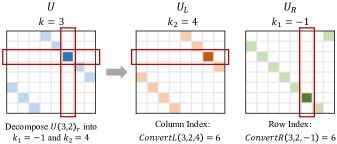
Figure 1: Example of ConvertR and ConvertL on an $8\times 8$ matrix

Now we have the fundamental rule to decompose each entry of $U$ into the desired diagonals of $U_{R}$ and $U_{L}$, but this alone is not sufficient to ensure overall correctness, which is only guaranteed when each row and column of $U_{R}$ and $U_{L}$ contains exactly one non-zero entry. Hence, what comes next is to examine potential conflicts (Definition 2), enumerated as follows:

• In $U_{R}$, row conflicts may occur, while column conflicts are impossible; conversely, in $U_{L}$, only column conflicts may occur. Furthermore, there exists a duality between $U_{R}$ and $U_{L}$: For any $k_{1},k_{2}=k-k_{1}$, $\texttt{ConvertL}(k,l,k_{2})=\texttt{ConvertL}(k,l,k-k_{1})=l+k-k_{1}=\texttt{ConvertR}(k,l,k_{1})$. This implies that managing either $U_{L}$ or $U_{R}$ is sufficient to ensure that the other matrix undergoes a symmetric process.

• Conflict can only exist between two different diagonals. Imagine if we use ConvertR to decompose all entries in $U$ onto the same diagonal in $U_{R}$, there would be no conflict, but such a decomposition is meaningless, as the number of non-zero diagonals in $U_{L}$ remains the same as in $U$.

Definition 2.

We say there is a row conflict (or column conflict) between two non-zero entries in a permutation matrix $U$ when they are in the same row (or column). Furthermore, there is a conflict between two non-zero diagonals in $U$ when there exists one or more pairs of conflicting entries on these diagonals.

3.2 Concrete Design

Based on the observation above, we design an algorithm for finding a depth-1 ideal decomposition for arbitrary $n\times n$ permutation matrices. The algorithm is composed of four steps listed below.

Step 1. We first set $U^{\prime}\leftarrow U-E$, where $E$ is a matrix of the same size as $U$, with the $0$-th diagonal matching that of $U$ and all other entries being zero. This step extracts all non-zero elements from the $0$-th diagonal of $U$ to avoid initial conflicts between the $\pm r_{c}$-th diagonal and the $0$-th diagonal of $U_{R}$ in Step 2.

Step 2. We proceed by decomposing each non-zero entry in $U^{\prime}$ to either $r_{c}$-th or $-r_{c}$-th diagonals of $U_{R}$, selecting the one closest to it ( with $r_{c}$ corresponding to $r_{c}^{(1)}$ in Definition 1) :

1. First, we create a set of tables representing the non-zero diagonals of $U_{R}$ determining the entries in $U^{\prime}$:

   $$M=\{M_{r_{c}},M_{-r_{c}},M_{0}\},$$

   where $M_{i}$, for $i\in\{\pm r_{c},0\}$, corresponds to the $i$-th non-zero diagonal in $U_{R}$, whose keys indicate the row coordinates of entries on it and the values store the diagonal coordinates of entries in $U^{\prime}$ determined by the keys.

2. Next, for each row coordinate $l$ of non-zero entries in the $k$-th diagonal of $U^{\prime}$, add the key-value pair $\big{(}\texttt{ConvertR}(k,l,r_{c}),k\big{)}$ to $M_{r_{c}}$ if $k>0$; otherwise, add $\big{(}\texttt{ConvertR}(k,l,-r_{c}),k\big{)}$ to $M_{-r_{c}}$.

This step provides an initial view of $U_{R}$ with non-zero entries precisely aligned on the $r_{c}$-th and $-r_{c}$-th diagonals but with potential conflicts between these diagonals.

Step 3. Now we try to solve the conflicts one by one. For each key-value pair $(a_{1},b_{1})$ in $M_{r_{c}}$, if a pair $(a_{1},b_{2})$ exists in $M_{-r_{c}}$ for some $b_{2}$, this implies a conflicts at row $a_{1}$ in $U_{R}$, and we do the following to find a solution:

1. If $|b_{1}|,|b_{2}|>r_{c}$, this implies that the entries in $U^{\prime}$ determined by $a_{1}$ and $a_{2}$ are so far away from the zero axis that the conflict cannot be resolved and the algorithm has to terminate.

2. If not, it implies that at least one conflicting entry corresponding to either the row index $a_{1}$ or $a_{2}$ can be moved to the zero axis of $U_{R}$. Then we create a set of arrays: $A=\{A_{diag},A_{key},A_{value},A_{key}^{new}\}$ for storing information of entries moved to the zero axis.

3. If $|b_{1}|\leq r_{c}$, we move entry $(a_{1},b_{1})$ from $M_{r_{c}}$ to $M_{0}$, and perform a recursive check for conflicts brought by this movement:

   1. Delete key-value pair $(a_{1},b_{1})$ from $M_{r_{c}}$, and add $(a_{0},b_{1})$ to $M_{0}$ where $a_{0}\leftarrow a_{1}+r_{c}$.

   2. Append $r_{c},a_{1},b_{1},a_{0}$ to $A_{diag},A_{key},A_{value},A_{key}^{new}$, respectively. This stores the movement information into $A$.

   3. Perform conflict check between $M_{0}$ and $M_{\pm r_{c}}$ recursively: $solved\leftarrow\texttt{CheckZero2RC}(M,a_{0},b_{1},n,A)$. We explain CheckZero2RC in Remarks 1.

4. If $solved\not=1$ and $|b_{2}|\leq r_{c}$, this implies that the conflict has not been resolved and we try moving entry $(a_{1},b_{2})$ from $M_{-r_{c}}$ to $M_{0}$:

   1. Delete key-value pair $(a_{1},b_{2})$ from $M_{r_{c}}$, and add $(a_{0},b_{2})$ to $M_{0}$ where $a_{0}\leftarrow a_{1}-r_{c}$.

   2. Append $-r_{c},a_{1},b_{2},a_{0}$ to $A_{diag},A_{key},A_{value},A_{key}^{new}$, respectively.

   3. $solved\leftarrow\texttt{CheckZero2RC}(M,a_{0},b_{2},n,A)$.

5. If $solved\not=1$, this implies that conflict still exists, and the algorithm has to terminate.

Remark 1.

For an entry in $U_{R}$ moved to the $0$-th diagonal, CheckZero2RC (Algorithm 1) do things recursively similar to Step 3, in the sense that it detects potential conflicts between $M_{0}$ and $M_{\pm r_{c}}$ brought by the movement, tries to resolve them by moving new conflicting entries to $M_{0}$ and invokes itself to further check these new movements (See if statements starting from line 2 and 12). Once CheckZero2RC encounters irresolvable conflicts, it undoes all actions of moving entries to $M_{0}$ recorded in $A$ (line 22 to 27).

Step 4. Generate $U_{L}$ according to $U^{\prime}$ and $U_{R}$ such that $U^{\prime}=U_{L}U_{R}$. One may replace $U^{\prime}$ with $U_{L}$ and update $r_{c}$ for the next round of decomposition.

Remark 2.

Note that although conflict resolution is only discussed for $U_{R}$, conflicts are symmetrically generated and resolved in $U_{L}$. Therefore, in the final step of the algorithm, we can deduce the conflict-free view of $U_{L}$ based on $U$ and $U_{R}$.

Algorithm 1 Check Conflicts Between the $0$-th and $\pm r_{c}$-th Diagonals (CheckZero2RC)

0:    $M=\{M_{r_{c}},M_{-r_{c}},M_{0}\}$: A set of tables identifying the current $U_{R}$’s view; $a_{0}$: The row index of the entry on the zero axis of $U_{R}$ to be checked;$b_{0}$: The diagonal of a entry in $U$, which is the determined by $U_{R}(a_{0},0)_{r}$; $n$: The dimension of $U$; $A$: The set of arrays storing the status of entries moved to the $0$-th diagonal.

0:    $solved\in\{0,1\}$: Indicates whether the conflict check is complete ($1$) or failed ($0$);

1:  $solved\leftarrow 1$

2:  if $a_{0}$ is in $M_{r_{c}}$ then

3:     $b_{1}\leftarrow M_{r_{c}}[a_{0}]$

4:     if $|b_{1}|>r_{c}$ then

5:        return  $0$

6:     end if

7:     $a_{0}^{new}=a_{0}+r_{c}\mod{n}$

8:     $M_{0}[a_{0}^{new}]\leftarrow b_{1}$

9:     Delete the key $a_{0}$ from $M_{r_{c}}$.

10:     Append $r_{c},a_{0},b_{1}$, and $a_{0}^{new}$ to $A_{diag},A_{key},A_{value}$, and $A_{key}^{new}$, respectively.

11:     $solved\leftarrow\texttt{CheckZero2RC}(M,a_{0}^{new},b_{1},n,A)$

12:  end if

13:  if $a_{0}$ is in $M_{-r_{c}}$ and $solved=1$  then

14:     $b_{2}\leftarrow M_{-r_{c}}[a_{0}]$

15:     if $|b_{2}|>r_{c}$ then

16:        return  $0$

17:     end if

18:     $a_{0}^{new}=a_{0}-r_{c}\mod{n}$

19:     $M_{0}[a_{0}^{new}]\leftarrow b_{2}$

20:     Delete the key $a_{0}$ from $M_{-r_{c}}$.

21:     Append $-r_{c},a_{0},b_{2}$, and $a_{0}^{new}$ to $A_{diag},A_{key},A_{value}$, and $A_{key}^{new}$, respectively.

22:     $solved\leftarrow\texttt{CheckZero2RC}(M,a_{0}^{new},b_{2},n,A)$

23:  end if

24:  if $solved\not=1$ then

25:     for $0\leq i<\text{len}(A_{sign})$ do

26:        Delete the key $A_{key}^{new}[i]$ from $M_{0}$.

27:        $M_{A_{diag}[i]}[A_{key}[i]]\leftarrow A_{value}[i]$

28:     end for

29:  end if

30:  return  $solved$

The proposed algorithm yields an approximate depth-1 ideal decomposition with negligible additional computational cost in terms of homomorphic evaluations for those input permutations containing a depth-$1$ decomposition solution (Theorem 2). The so-called additional computation corresponds to $E$ we extract from the input permutation in Step 1. If the algorithm can be recursively applied to the permutation $\ell\leq\log{n}-1$ times, then we have the following equation:

$$U=(((U_{L_{\ell}}U_{R_{\ell}}+E_{\ell})U_{R_{\ell-1}}+E_{\ell-1})\dots)U_{R_{1}}+E_{1},$$ (6)

where the total computational cost for homomorphic masking is less than one ciphertext rotation, thus yielding a marginal effect.

In the next section, our proposed algorithm is applied to specific permutations in homomorphic matrix operations, where we provide a visualizable demonstration of this procedure.

Theorem 2.

For any given $n\times n$ permutation matrix $U$, if there exists a depth-1 ideal decomposition $f$ of $U$ where $f:U=U_{L}U_{R}$ satisfies that each non-zero entry of $U$ is determined by only two diagonals from $U_{L}$ and $U_{R}$, respectively, then the proposed algorithm outputs a decomposition $U=U_{L}^{\prime}U_{R}^{\prime}+E$ with $U^{\prime}=U_{L}^{\prime}U_{R}^{\prime}$ a depth-$1$ ideal decomposition and $E=U\otimes I$ with $\otimes$ representing entry-wise multiplication.

Proof.

We can directly extract, or remove, $E$ from $U_{L}$ and $U_{R}$ without altering the diagonal distribution of these matrices: for each non-zero entry $E(0,\ell)_{r}$ in $E$, exactly one among the three pairs of entries:

$$\begin{split}&\big{[}U_{L}(0,\ell)_{r},U_{R}(0,\ell)_{r}\big{]},\\ &\big{[}U_{L}(-r_{c},\ell)_{r},U_{R}(r_{c},\texttt{ConvertR}(0,\ell,r_{c}))_{r}\big{]},\\ &\big{[}U_{L}(r_{c},\ell)_{r},U_{R}(-r_{c},\texttt{ConvertR}(0,\ell,-r_{c}))_{r}\big{]}\end{split}$$ (7)

is set with the value $(1,1)$, and we remove it from $U_{L}$ and $U_{R}$ respectivley. The newly obtained matrices $U_{L}^{(1)}$ and $U_{R}^{(1)}$ satisfy the equation $U=U_{L}^{(1)}U_{R}^{(1)}+E=U^{\prime}+E$.

On the other hand, assuming $U^{\prime}$ has at least one $1$-ideal solution $U^{\prime}=U_{L}^{(1)}U_{R}^{(1)}$, the proposed algorithm finds one such solution. It suffices to prove that resolving each conflict is independent of the others and that the algorithm exhausts all means of resolving each conflict until they are resolved. According to Theorem 1, entries on the diagonal of $U^{\prime}$ (denoted as $k$) with absolute values less than $r_{c}$ can be decomposed onto the $\text{sign}(k)\cdot r_{c}$ diagonal or the $0$ diagonal of $U_{R}$, while entries with absolute values greater than $r_{c}$ can only be decomposed onto the $\text{sign}(k)\cdot r_{c}$ diagonal of $U_{R}$. Our algorithm in Step 1 decomposes all entries onto the $\text{sign}(k)\cdot r_{c}$ diagonal of $U_{R}$, and when resolving any conflict on these two diagonals, it only reduces the number of non-zero entries they contain. Therefore, resolving conflicts between the $r_{c}$ and $-r_{c}$ diagonals is independent of each other. When resolving each conflict, the algorithm always attempts to move entries on the $r_{c}$ diagonal first, recursively resolving conflicts brought by moving entries to the $0$ diagonal, and if it encounters an irresolvable conflict, it undoes all operations and attempts the same for entries on the $-r_{c}$ diagonal, thus exhaustively resolving conflicts.

∎

4 Full-depth Decomposability on Specific Permutations

In this section, we demonstrate that certain permutations can be ideally decomposed in full-depth as per Definition 1. These permutations originate from Jiang et al.’s HMT scheme [6] and the HMM algorithm by Rizomiliotis and Triakosia [16]. Our thought process was as follows: we first applied the depth-$1$ decomposition searching algorithm from Section 3 to the permutation used in Jiang et al.’s implementation of HMT, through which we discovered the full-depth decomposition method for this permutation. We then further reduced the permutation from Rizomiliotis and Triakosia’s HMM to the former, thereby illustrating that the full-depth decomposition method is applicable to all such permutations.

4.1 Permutation for Homomorphic Matrix Transposition

Let $ct(\mathbf{a})$ denote a ciphertext encrypting the $n$-dimensional vector $\mathbf{a}$, where $\mathbf{a}$ is the row-ordering encoding of a $d\times d$ matrix $A$. To obtain the ciphertext of the row-ordering vector of $A^{T}$, a specific homomorphic permutation (denoted as $U^{t}$) is applied to $ct(\mathbf{a})$. The $d^{2}\times d^{2}$ matrix $U^{t}$ possesses $2d-1$ nonzero diagonals, whose indices (denoted as $k$) are distributed in an arithmetic sequence $k=(d-1)\cdot i,i\in\mathbb{Z}\cap(-d,d)$. The row coordinates (denoted as $l$) of the nonzero entries on the $(d-1)\cdot i$ diagonal are distributed as follows:

$$\{l=(d+1)\cdot j+i,0\leq j<d-i\}$$ (8)

for $i\geq 0$, or:

$$\{l=(d+1)\cdot j+i,i\leq j<d\}$$ (9)

for $i<0$. Subsequently, we will first consider the case where $d$ is a power of $2$ and then proceed to a more generalized context for the decomposition of $U^{t}$.

4.1.1 Case with Dimension a Power of $2$

$U^{t}$ can be precisely decomposed into $U^{t}_{L}U^{t}_{R}$ when we apply the depth-$1$ decomposition searching algorithm proposed in Section 3. This application on a $16\times 16$ $U^{t}$ is illustrated in Figure 2. Here, we skip the algorithm’s first step, as the non-zero elements along the zero-axis in $U^{t}$ actually do not create any conflicts.

Step 2 of the algorithm is shown in Figure 2b. Leveraging the fact that the indices of non-zero diagonals in $U^{t}$ has a common difference of $d-1$, we set $r_{c}=(d-1)\cdot\lceil\frac{d-1}{2}\rceil$, which is 6 in this case. We can observe that all non-zero elements in $U^{t}$ are decomposed onto the $6$th and $-6$th diagonals of $U^{t}_{R}$ (ignoring those on the zero-axis), which introduces conflicts in rows 7 and 8. In Figure 2c, we see how the searching algorithm resolves these conflicts from Step 2, illustrated by the dashed paths. For example, in row 8, the conflicting entry on the 3rd diagonal of $U^{t}$ at the 11th position shifts from the 6th diagonal to the 0th diagonal in $U^{t}_{R}$, which then conflicts with an entry on the 3rd diagonal in row 14. This results in $U^{t}_{R}(3,14)_{r}$ being forced onto the zero-axis, yet without triggering further conflicts.

Once we solve all the conflicts in $U^{t}_{R}$, we use it and $U^{t}$ to get $U^{t}_{L}$ such that $U^{t}=U^{t}_{L}U^{t}_{R}$ (Figure 2d). It is interesting that both of these factors exhibit good structural properties.

(a) $16\times 16$ $U^{t}$ with $1$s painted in dark blue.

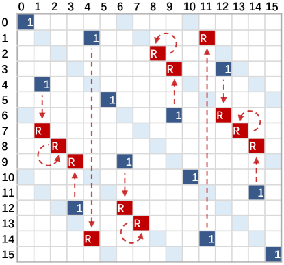
(b) Step 2. Red entries denote the $1$s in $U^{t}_{R}$ after Step 2

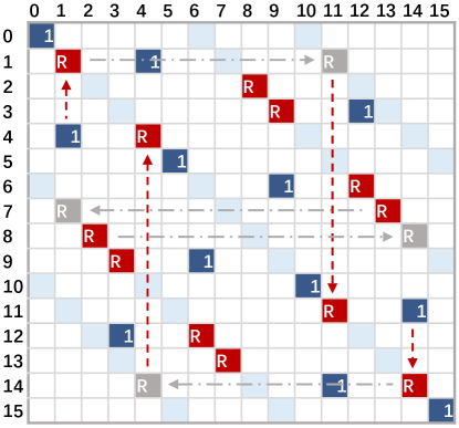
(c) Step 3. Conflicting entries moved away are painted in grey

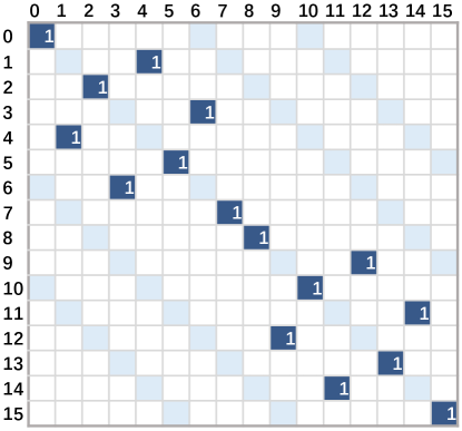
(d) Step 4. $U^{t}_{L}$ constructed through $U^{t}_{R}$ and $U^{t}$

Figure 2: Applying depth-1 ideal decomposition search to $U^{t}$ of size $16\times 16$

If we let $A$ be evenly partitioned into $4$ blocks with size $d/2\times d/2$:

$$A=\left[\begin{matrix}{A^{\prime}_{0,0}}&{A^{\prime}_{0,1}}\\ {A^{\prime}_{1,1}}&{A^{\prime}_{1,1}}\\ \end{matrix}\right].$$ (10)

Then the effect of $U^{t}_{R}$ and $U^{t}_{L}$ can be expressed as follows:

$$\left[\begin{matrix}{A^{\prime}_{0,0}}&{A^{\prime}_{1,0}}\\ {A^{\prime}_{0,1}}&{A^{\prime}_{1,1}}\\ \end{matrix}\right]\leftarrow U^{t}_{R}(A),\left[\begin{matrix}{A^{\prime}_{0,0}}^{T}&{A^{\prime}_{1,0}}^{T}\\ {A^{\prime}_{0,1}}^{T}&{A^{\prime}_{1,1}}^{T}\\ \end{matrix}\right]\leftarrow U^{t}_{L}\left(U^{t}_{R}(A)\right),$$ (11)

Equation 11 indicates that $U^{t}_{R}$ swaps the positions of $A^{\prime}_{0,1}$ and $A^{\prime}_{1,0}$, while $U^{t}_{L}$ performs block-wise transposition. This follows that:

$$A^{T}=U_{L_{\ell}}^{t}\left(U_{R_{\ell}}^{t}\left(\dots\left(U_{R_{1}}^{t}(A)\right)\right)\right)$$ (12)

holds for $\ell\leq\log{d^{2}}-1$ if the following process defines the permutations in it:

1. Before each $U^{t}_{R_{i}}$ takes place, each block in $A$ is evenly partitioned into $4$ sub-blocks, where the initial block is of size $d\times d$. The sub-blocks are interpreted as blocks in the next partition before $U^{t}_{R_{i+1}}$. No partition is done after $U^{t}_{R_{\ell}}$.

2. $U^{t}_{R_{i}}$ swaps the sub-blocks at positions $[0,1]$ and $[1,0]$ in each block of $A$.

3. $U^{t}_{L_{\ell}}$ performs block-wise transposition.

Remark 3.

The conditions above implies that $U^{t}_{R_{i}}$ swaps $d/2^{i}$-size sub-blocks inside each $d/2^{i-1}$-size block, and $U^{t}_{L_{\ell}}$ transposes each $d/2^{\ell}$-size block, for $1\leq i\leq\ell$.

The non-zero diagonals of $U^{t}_{R_{i}}$ are precisely distributed at $\{0,\pm(d-1)d/2^{i}\}$ for $1\leq i\leq\ell$ according to Theorem 3 and Theorem 4. $U^{t}_{L_{\ell}}$ swaps the entries at positions $[q,p]$ and $[p,q]$ for $0\leq p,q<d/2^{\ell}$ in each $d/2^{\ell}$-size block. These entry swappings correspond to non-zero diagonals with indices:

$$\begin{split}&\{0,\pm d(q-p)+p-q\mid 0\leq p,q<d/2^{\ell}\}=\\ &\{0,\pm 1\cdot(d-1),\pm 2\cdot(d-1),\dots,\pm(d/2^{\ell}-1)\cdot(d-1)\}.\end{split}$$ (13)

Now, it is evident that Equation 12 with $U^{t}_{R_{i}}$ and $U^{t}_{\ell}$ satisfying the correctness requirements above is a depth-$\ell$ decomposition of $U^{t}$ for $1\leq\ell\leq\log{d^{2}}-1$.

Theorem 3.

For any square matrix of arbitrary size, the permutation matrix corresponding to swapping any two blocks (square submatrices) of the same size contains at most three nonzero diagonals.

Proof.

Given $A$ is of size $d\times d$, and the two blocks to be swapped are of size $d^{\prime}\times d^{\prime}$, where $d^{\prime}<d$. If $A^{\prime}_{i,j}[0,0]=A[p,q]$ and $A^{\prime}_{k,l}[0,0]=A[u,v]$, then:

$$\begin{split}A^{\prime}_{i,j}[x,y]=A[p+x,q+y],\\ A^{\prime}_{k,l}[x,y]=A[u+x,v+y].\end{split}$$ (14)

Let $\text{offset}=(u+x)d+(v+y)-(p+x)d-(q+y)=d(u-p)+(v-q)$. Assume that the position of $A[p+x,q+y]$ on vector $\mathbf{a}$ is to the left of the position of $A[u+x,v+y]$, then the former needs to be rotated $\text{offset}\bmod{n}$ steps to reach the latter’s position, and the latter needs to be rotated $-\text{offset}\bmod{n}$ steps to reach the former’s position, independent of $x$ and $y$. All other entries outside the two blocks to be swapped maintain their original positions. Therefore, the swap of the two blocks involves at most three non-zero diagonals. ∎

Theorem 4.

Given any square matrix of arbitrary size, when performing the same permutation on different fixed-size submatrices, the number and positions of the diagonals in the corresponding permutation matrix remain unchanged.

Proof.

Let $A$ be a matrix of size $d\times d$, and let $A^{\prime}$ with $A^{\prime}[0,0]=A[s,t]$ be any submatrix of $A$ with size $d^{\prime}\times d^{\prime}$, where $d^{\prime}\leq d$. For any two entries in $A^{\prime}$, located at $A^{\prime}[p,q]$ and $A^{\prime}[u,v]$, we have:

$$\begin{split}A^{\prime}[p,q]=A[s+p,t+q]\\ A^{\prime}[u,v]=A[s+u,t+v]\end{split}$$ (15)

To move $A^{\prime}[p,q]$ to the position of $A^{\prime}[u,v]$, it requires a rotation of $d(s+u)+(t+v)-d(s+p)-(t+q)=d(p-u)+(q-v)$ steps. It is evident that the number of rotation steps for movements within the block is independent of the block’s position within $A$. ∎

4.1.2 Case with Arbitrary Dimension

For the dimension $n=d^{2}$ of $U^{t}$ that is not a power of $2$, there exists a unique set of prime numbers $\{p_{i}\mid 0\leq i<\alpha\}$ such that $n=\prod_{i=0}^{\alpha-1}p_{i}^{k_{i}},(k_{i}>0)$. Assume that $2$ is in the set and denoted as $q_{0}$, then $U^{t}$ can only be decomposed at most $k_{0}$ rounds using $U^{t}_{R_{i}}$ and $U^{t}_{L_{k_{0}}}$ defined in Section 4.1.1. After this, the blocks in $A$ cannot be evenly partitioned into $4$ sub-blocks for further decomposition.

The simplest solution we can find is to use zero-padding to extend the dimensions of the matrix to be transposed into powers of two. Let the original dimension of the matrix $A$ be $d$, and there exists an integer $i$ such that $2^{i-1}<d<2^{i}$. By extending $A$ into a $2^{i}\times 2^{i}$ matrix, the corresponding $U^{t}$ can undergo an ideal decomposition of depth $i-1$. This requires approximately $(3-1)\cdot(i-1)$ ciphertext rotation operations. In the worst-case scenario where $d$ is only slightly greater than $2^{i-1}$, zero-padding will expand the space of $A$ by approximately $4$ times, but the decomposition depth only increases by $1$. It is worth noting that popular RLWE-based homomorphic encryption schemes like CKKS typically use vector spaces with dimensions that are powers of $2$ as plaintext spaces, so the zero-padding strategy aligns well with current homomorphic encryption schemes.

However, we do find alternative solutions to avoid the spatial cost, which can accommodate homomorphic encryption schemes like BGV that allow more flexible adjustments of the plaintext space. The idea is to define a new partition for odd-dimensional blocks. Below, we explain this with an example of a single round of $U^{t}$ decomposition for odd dimensions.

First, we define an unequal partition for any $d\times d$ matrix $A$ to be transposed, where $d$ is an odd number expressed as $2\cdot d^{\prime}+1$ for some $0\leq d^{\prime}$. $A$ is also considered as any block in the matrix to be decomposed. Let:

$$\begin{array}[]{ll}B^{\prime}_{0,0}=\left[\begin{matrix}A[i,j]\end{matrix}\right]_{0\leq i\leq d^{\prime}}^{0\leq j\leq d^{\prime}}&B^{\prime}_{0,1}=\left[\begin{matrix}A[i,j]\end{matrix}\right]_{0\leq i\leq d^{\prime}-1}^{d^{\prime}+1\leq j\leq 2d^{\prime}}\\ \\ B^{\prime}_{1,0}=\left[\begin{matrix}A[i,j]\end{matrix}\right]_{d^{\prime}+1\leq i\leq 2d^{\prime}}^{0\leq j\leq d^{\prime}-1}&B^{\prime}_{1,1}=\left[\begin{matrix}A[i,j]\end{matrix}\right]_{d^{\prime}\leq i\leq 2d^{\prime}}^{d^{\prime}\leq j\leq 2d^{\prime}}\end{array},$$

then the unequal partition of $A$ is given as follows:

$$A=\begin{bmatrix}B^{\prime}_{0,0}&B^{\prime}_{0,1}\\ B^{\prime}_{1,0}&B^{\prime}_{1,1}\end{bmatrix}.$$ (16)

Here, $A$ is partitioned into four blocks, with an overlapping part $A[d^{\prime},d^{\prime}]$ between $B^{\prime}_{0,0}$ and $B^{\prime}_{1,1}$. After designing the partitioning method for odd-dimensional blocks, we then redefine the permutation in Equation 12 to ensure the equation holds for $A$ with arbitrary dimension:

1. Before each $U^{t}_{R_{i}}$ takes place, each block in $A$ is partitioned into $4$ sub-blocks, where the initial block is of size $d\times d$. For blocks with odd dimensions, the partition follows Equation 16. The sub-blocks are interpreted as blocks in the next partition before $U^{t}_{R_{i+1}}$. No partition is done after $U^{t}_{R_{\ell}}$.

2. $U^{t}_{R_{i}}$ swaps the sub-blocks at positions $[0,1]$ and $[1,0]$ in each block.

3. $U^{t}_{L_{\ell}}$ performs block-wise transposition.

In any partitioning round, the blocks in $A$ have at most two dimensions differing by at most 1 (Theorem 5). In this case, the number of non-zero diagonals involved in the block-wise permutation is the union of the non-zero diagonals required for the permutation on blocks of different sizes. Thus, for $0\leq i\leq\ell$, the maximum number of non-zero diagonals in each $U^{t}_{R_{i}}$ increases from 3 to 5. The number of non-zero diagonals of $U^{t}_{L_{\ell}}$ remains $O(d/2^{\ell-1})$ for $\ell\leq\lfloor\log{d}\rceil-1$. Such decomposition only approximates the ideal form with each $U^{t}_{R_{i}}$ having two additional non-zero diagonals. Nevertheless, it avoids the up to fourfold spatial cost of the zero-padding strategy mentioned earlier.

Theorem 5.

Let $A$ be any square matrix of size $d\times d$ and its initial block size is $d\times d$. Define one round of block partitioning as follows: each block of $A$ with an odd dimension is partitioned and recombined according to equations 16, while each block with an even dimension is partitioned according to equation 10. After any number of rounds of partitioning, $A$ contains blocks of at most two different sizes which differ by only $1$.

Proof.

Suppose that after a certain round of partitioning, the blocks in $A$ have dimensions differing by 1, specifically $d^{\prime}$ and $d^{\prime}+1$. After the next round of partitioning, if $d^{\prime}$ is odd, the blocks of dimension $d^{\prime}$ are divided into blocks of dimensions $\frac{d^{\prime}+1}{2}-1$ and $\frac{d^{\prime}+1}{2}$, while the blocks of dimension $d^{\prime}+1$ are divided into blocks of dimension $\frac{d^{\prime}+1}{2}$. If $d^{\prime}$ is even, the blocks of dimension $d^{\prime}+1$ are divided into blocks of dimensions $\frac{d^{\prime}}{2}+1$ and $\frac{d^{\prime}}{2}$, while the blocks of dimension $d^{\prime}$ are divided into blocks of dimension $\frac{d^{\prime}}{2}$. Given that the two block dimensions initially produced by Equations 16 differ by only 1, by mathematical induction, after each round of partitioning, the blocks in $A$ always have only two different dimensions, differing by only 1. ∎

4.2 Permutations for Homomorphic Matrix Multiplication

It is intriguing that we observe permutations with structures similar to $U^{t}$ in Rizomiliotis and Triakosia’s HMM algorithm. We can achieve an asymptotically faster homomorphic matrix multiplication by applying the decomposition strategy for $U^{t}$ to these permutations. Furthermore, we present methods to reduce the multiplication depth to a constant level and to enhance the utilization of the encoding space.

Let us first briefly describe Rizomiliotis and Triakosia’s scheme. Let $A$ and $B$ be the $d\times d$ matrices to be multiplied, and let the plaintext space be a vector space of dimension $n=d^{3}$. The method proposed by Rizomiliotis and Triakosia first appends $(d-1)$ zero matrices of size $d\times d$ to both the end of $A$ and $B$ along the column to form $\hat{A}$ and $\hat{B}$ of size $d^{2}\times d$, allowing them to be packed into plaintext vectors. Two permutations $U^{\gamma}$ and $U^{\xi}$ are then applied to $\hat{A}$ and $\hat{B}$ respectively (these correspond to Algorithm A and B in the original work, which readers can refer to for details). Next, column-wise replication is performed on $U^{\gamma}(\hat{A})$ and row-wise replication on $U^{\xi}(\hat{B})$, and denote the replicated results as $\tilde{A}$ and $\tilde{B}$ respectively. Finally, compute $\hat{C}=\tilde{A}\otimes\tilde{B}$, and perform $\hat{C}\leftarrow\texttt{Rot}(\hat{C},d^{3}/2^{i})+\hat{C}$ for $1\leq i\leq\log{d}$. This yields the desired result $C=AB$ in the first $d\times d$ block of $\hat{C}$.

Rizomiliotis and Triakosia consider that both $U^{\gamma}$ and $U^{\xi}$ require $d$ ciphertext rotations, dominating the overall algorithm complexity. We will explain that these two permutations can be ideally decomposed to achieve an asymptotically faster speed.

4.2.1 Decomposability of $U^{\gamma}$ and $U^{\xi}$

For $U^{\gamma}$, it can be fully regarded as a transposition acting on a $d\times d$ matrix where each entry is a $d\times 1$ vector:

$$\begin{split}&\hat{A}=\left[\begin{matrix}\mathbf{a}_{0}&\cdots&\mathbf{a}_{d-1}\\ \mathbf{0}_{c}&\cdots&\mathbf{0}_{c}\\ \vdots&\ddots&\vdots\\ \mathbf{0}_{c}&\cdots&\mathbf{0}_{c}\\ \end{matrix}\right],U^{\gamma}(\hat{A})=\left[\begin{matrix}\mathbf{a}_{0}&\mathbf{0}_{c}&\cdots&\mathbf{0}_{c}\\ \vdots&\vdots&\ddots&\vdots\\ \mathbf{a}_{d-1}&\mathbf{0}_{c}&\cdots&\mathbf{0}_{c}\\ \end{matrix}\right],\\ &\mathbf{a}_{i}=\left[\begin{matrix}A[0,i]&\cdots&A[d-1,i]\end{matrix}\right]^{T},\text{for}\phantom{a}0\leq i<d.\end{split}$$ (17)

In the previous section, we discussed that the basic unit of a matrix (whether a vector or a single value) does not affect the number of non-zero diagonals involved in block-wise permutations. Thus, the decomposition of $U^{t}$ directly applies to $U^{\gamma}$. Specifically, when $d$ is a power of two, $U^{\gamma}$ has a depth-$\ell$ ideal decomposition for $\ell\leq\log{d}-1$. When $d$ is set arbitrarily, $U^{\gamma}$ has an approximate depth-$\ell$ ideal decomposition for $\ell\leq\lfloor\log{d}\rceil-1$.

Furthermore, we can modify the decomposition of $U^{\gamma}$ to achieve constant multiplication depth. We fill the non-zero diagonals of $U^{\gamma}$ with ones and denote the result as $U^{\gamma}_{pad}$. At this point, $U^{\gamma}_{pad}(\hat{A})$ is the sum of the rotated $\hat{A}$ by steps of $0,-(d^{2}-1),\dots,-(d^{2}-1)(d-1)$ without any masking. It can be observed that $U^{\gamma}_{pad}(\hat{A})$ has the same first column as $U^{\gamma}(\hat{A})$. This implies that we can use $U^{\gamma}_{pad}(\hat{A})$ with one masking in the end to get the result of $U^{\gamma}(\hat{A})$.

Let us explain the reasons behind such a phenomenon. For $U^{\gamma}(\hat{A})$, entries of $A$ in $\hat{A}$ are rotated by $-k(d^{2}-1)$ steps ($0\leq k<d$) to ensure those in equivalence class $i\bmod{d}$ are shifted to equivalence class $0\bmod{d}$. Since $(d^{2}-1)$ is coprime to $d$, for each equivalence class $i\bmod{d}$, there is exactly one unique $k$ such that $i+k=0\bmod{d}$. This implies that during each rotation by steps $0,-(d^{2}-1),\dots,-(d^{2}-1)(d-1)$, only one equivalence class is rotated to the first column position of $\hat{A}$.

The decomposition of $U^{\gamma}_{pad}$ can be directly obtained by filling all non-zero diagonals in the permutation matrices of $U^{\gamma}$’s decomposition with ones, yielding a constant multiplication depth of $1$.

Similarly, $U^{\xi}$ can be interpreted as a transposition acting on a $d\times d$ matrix where each basic unit is a $1\times d$ vector:

$$\begin{split}&\hat{B}=\left[\begin{matrix}\mathbf{b}_{0}&\cdots&\mathbf{b}_{d-1}\\ \mathbf{0}_{r}&\cdots&\mathbf{0}_{r}\\ \vdots&\ddots&\vdots\\ \mathbf{0}_{r}&\cdots&\mathbf{0}_{r}\\ \end{matrix}\right],U^{\xi}(\hat{B})=\left[\begin{matrix}\mathbf{b}_{0}&\mathbf{0}_{r}&\cdots&\mathbf{0}_{r}\\ \vdots&\vdots&\ddots&\vdots\\ \mathbf{b}_{d-1}&\mathbf{0}_{r}&\cdots&\mathbf{0}_{r}\\ \end{matrix}\right],\\ &\mathbf{b}_{i}=\left[\begin{matrix}B[i,0]&\cdots&B[i,d-1]\end{matrix}\right],\text{for}\phantom{a}0\leq i<d.\end{split}$$ (18)

Thus, $U^{\xi}$ can be decomposed following the decomposition method of $U^{t}$. We can also fill non-zero diagonals with ones to achieve a constant multiplication depth. The correctness of this approach is consistent with the discussion for $U^{\gamma}$ above: $U^{\xi}(\hat{B})$ requires moving $\mathbf{b}_{i}$ in $\hat{B}$ by $k(d-1)$ positions (with $1\times d$ vectors as units) to the column indexed by 0, where $0\leq i,k<d$. For each $\mathbf{b}_{i}$, there is exactly one unique $k$ such that $i+k(d-1)=0\mod d$. This implies that during the rotations of $\hat{B}$ by steps of $0,-(d-1),\dots,-(d-1)^{2}$, each rotation carries exactly one $\mathbf{b}_{i}$ to the first column position.

4.2.2 Flexible Utilization of the Encoding Space

The original algorithm by Rizomiliotis and Triakosia necessitates a plaintext encoding space of at least $d^{3}$ to perform $d\times d$ matrix multiplication, resulting in an exponential computational overhead for HMM as $d$ increases, eventually becoming intolerable. Here, we propose a strategy that offers a balanced trade-off between encoding space and computational efficiency. In essence, we decompose $U^{\gamma}(\hat{A})$ and $U^{\xi}(\hat{B})$ each into $d/d^{\prime}$ matrices, thereby reducing the encoding space required for representing $A$ and $B$ to $d^{2}\cdot d^{\prime}$, allowing larger matrices to be accommodated within a single ciphertext.

Let $d^{\prime}$ be a divisor of $d$. For any matrices $\hat{A}$ and $\hat{B}$ involved in matrix multiplication, they are both interpreted as the concatenation of $d/d^{\prime}$ blocks as follows:

$$\hat{G} =\left[\begin{array}[]{c|ccc|c}\cdots&\mathbf{g}_{d^{\prime}k}&\cdots&\mathbf{g}_{d^{\prime}(k+1)-1}&\cdots\\ \cdots&\mathbf{0}&\cdots&\mathbf{0}&\cdots\\ \cdots&\vdots&\ddots&\vdots&\cdots\\ \cdots&\mathbf{0}&\cdots&\mathbf{0}&\cdots\\ \end{array}\right]{(0\leq k<\frac{d}{d^{\prime}})}$$ (19)

$$=\left[\begin{matrix}\hat{G}^{\prime}_{0}&\hat{G}^{\prime}_{1}&\cdots&\hat{G}^{\prime}_{\frac{d}{d^{\prime}}-1}\end{matrix}\right],$$

where $\mathbf{g}_{i}=\mathbf{a}_{i}$ (or $\mathbf{b}_{i}$) and $\mathbf{0}=\mathbf{0}_{c}$ (or $\mathbf{0}_{r}$). To complete the HMM, we apply block-wise $U^{\gamma}$ and $U^{\xi}$ to $\hat{A}$ and $\hat{B}$, respectively, and denote the results as: $U^{\gamma^{\prime}}(\hat{A})=[U^{\gamma}(\hat{A}^{\prime}_{0})\ldots U^{\gamma}(\hat{A}^{\prime}_{\frac{d}{d^{\prime}}-1})]$, $U^{\xi^{\prime}}(\hat{B})=[U^{\xi}(\hat{B}^{\prime}_{0})\ldots U^{\xi}(\hat{B}^{\prime}_{\frac{d}{d^{\prime}}-1})]$. According to Theorem 4, the complexity is $2\log{d^{\prime}}$ for processing both $\hat{A}$ and $\hat{B}$. Then, we use masking to extract each block $U^{\gamma}(\hat{A}^{\prime}_{i})$ (or $U^{\xi}(\hat{B}^{\prime}_{i})$) as an individual ciphertext, applying block-wise replication and column-wise replication within each block to obtain $\tilde{A}_{i}$ (or $\tilde{B}_{i}$). We then compute $\hat{C}=\sum_{i=0}^{\frac{d}{d^{\prime}}-1}\tilde{A}_{i}\otimes\tilde{B}_{i}$, followed by a summation over $O(\log d^{\prime})$ rotations on $\hat{C}$ to yield the final result. The total number of rotations is $O(3\log d^{\prime}+2\frac{d}{d^{\prime}}\log d)$.

5 New Design for Approximate Ideal Decomposition of Arbitrary Permutation

As previously mentioned, the idea of ideal decomposition aims to establish an upper bound for decomposition techniques. This bound can indeed be achieved for specific permutations. However, not all permutations can be ideally decomposed, especially those without strong structural properties. The depth-1 decomposition search algorithm we proposed earlier struggles to find solutions for randomly generated permutations.

The Benes network-based permutation decomposition [13] combined with the optimal level-collapsing strategy proposed by Halevi et al. [4] can construct a decomposition chain with depth $\log{n}-1$ for any given permutation, where each factor contains approximately 6 to 7 non-zero diagonals on average. Although this already offers a close approximation to ideal decomposition, we aim to present a new solution that performs better than such approximation when the number of available rotation keys is minimal.

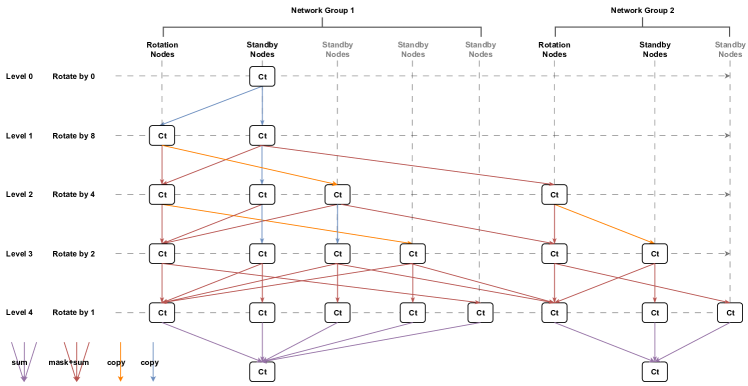
Figure 3: New network design for computing arbitrary homomorphic permutation (using length 16 as an example)

5.1 Overall Design

Our initial design conceptualizes permutations as a directed graph network (Figure 3). It consists of four major components:

• Nodes. The nodes in the network are categorized into two types: rotation nodes and standby nodes, both taking vectors as input. Rotation nodes rotate the input vector by certain steps, while standby nodes output the input vector unchanged.

• Edges. Edges transmit the output vector of one node, applying a mask before passing it to another node. When multiple edges converge at the same node, the vectors carried by these edges are summed together to form the input to that node.

• Levels. Levels correspond to the sequence in which nodes are processed, with nodes at the same level being handled concurrently.

• Groups. The network is vertically divided into several groups, each containing a column of rotation nodes and multiple columns of standby nodes. Nodes are processed first by iterating through levels, and then by group indices. The network’s final output is the sum of the bottom nodes’ output in all groups.

Such a network directs entries of the input vector to different paths for processing, eventually gathering them to form the permuted vector. We outline the method of constructing a network for any given permutation. Note that generating the network simulates the permutation process on an input vector.

Initially, the network contains a single standby node located at the $0$-th level of the $0$-th group, which stores all entries of the input vector. Each entry is marked with an “unsolved” tag, indicating that it has not yet been rotated to its target position. The network is then constructed group by group. For $i_{g}\geq 0$, the $i_{g}$-th group is constructed as follows.

A group is built level by level, starting from the minimum level containing unsolved entries. The following actions are taken in the iteration of level $\ell\geq 0$. For all unsolved entries at level $\ell$, we obtain the maximum remaining rotation distance $rot_{max}$ and let $rot$, the rotation step for the rotation node at level $\ell+1$, be the largest value among the powers of two smaller than $rot_{max}$ and $0$. Then, for each unsolved entry at level $\ell$, perform the following steps:

Step 1. Retrieve the entry’s remaining rotation distance $r_{rem}$, its original total rotation distance $r_{org}$, and its initial position $i$ in the original vector. These values determine the entry’s destination node at the next level. Calculate $i_{dst}=i+(r_{org}-r_{rem})\bmod{n}$, which gives its position in the next level’s node.

Step 2. If $r_{rem}\geq rot$, it should go to a rotation node. Check whether the $i_{dst}$-th position of the rotation at level $\ell+1$ in the current group is occupied.

• If not, allow the entry to occupy this position. To do so, set the $i_{dst}$-th position of the mask on the edge connecting the entry’s current node to the rotation node to 1, and update $r_{rem}\leftarrow r_{rem}-\text{rot}$.

• If it is occupied, compare the total rotation distance of the current entry and the occupying entry, letting the entry with the greater total rotation distance retain the position. If necessary, remove the occupying entry by undoing all previous modifications corresponding to its occupation and changing its tag from “unsolved” to “deferred,” indicating that it will move to the level $\ell+1$ in a future group.

Step 3. Otherwise, it should go to a standby node. Check whether the entry’s current node is a rotation node or a standby node.

• If it is a rotation node, get the count $m$ of standby nodes at level $\ell$, and allow the entry to occupy the $i$-th position of the $(m+1)$-th standby node at level $\ell+1$, setting the $i_{dst}$-th position of the mask on the edge connecting the two nodes to 1.

• If it is a standby node, let the entry occupy the standby node at level $\ell+1$ with the same index by setting the $i_{dst}$-th position of the mask on the edge connecting the two nodes to 1.

After completing the traversal, check if $\text{rot}=0$. If not, increment $\ell$ by 1 and move to the next level’s iteration. Otherwise, consider the current group’s construction complete, changing the tag of entries marked “unsolved” to “solved” and those marked “deferred” to “unsolved.” Proceed to the construction of the $i_{g}+1$-th group.

5.2 Technical Detail

We move on to present the key features and techniques of our proposed network construction for the homomorphic permutation.

5.2.1 Multi-group Network Construction

Groups with larger indices are generated to resolve occupation conflicts at the rotation nodes. This inevitably introduces additional rotation operations. Therefore, our design aims to keep the size of newly created groups as small as possible. This idea corresponds to several details in generating new groups:

Firstly, For any entry encountering an occupation conflict, we acknowledge the rotations it has already undergone and transfer it to one of the subsequent groups with a cross-group edge. Such a strategy bounds the number of levels by $\log{n}+1-i$ for any group in the network, where $i$ is the minimum source level (index) of entries it will receive.

Secondly, since entries with fewer total rotation steps tend to go through rotation nodes closer to the bottom of the network, prioritizing their removal when conflicts occur helps control conflicts in the next network at a lower level. This, together with the first details, further controls the number of levels of groups in a descending trend.

Thirdly, when an entry is tagged ”deferred”, its source address does not change until it successfully enters a group where it can be rotated at least once. This is to handle situations where an entry moved from the $k$-th group to the $(k+1)$-th group immediately encounters another occupation conflict, forcing it to move again to the $(k+2)$-th group. Since the entry did not undergo any rotation in group $(k+1)$, the edge carrying it should be established between group $k$ and group $(k+2)$.

5.2.2 Reduction of Masks and Depth

Many masks within our network are unnecessary when computing homomorphic permutations. They can be replaced with copy operations without compromising the correctness of the network.

For any group with a maximum level index of $\ell$, the unnecessary masks are those on edges reaching standby nodes, except for the edges from level $\ell-2$ to level $\ell-1$. This corresponds to the yellow and blue edges in diagram 3. Reducing them to copy operations allows us to eliminate a significant number of plaintext-ciphertext multiplications and reduce the multiplication depth of the overall network to at most $\log{n}-1$, which aligns with our definition of the ideal decomposition.

5.2.3 Timing of Rescale

Rescale is the most computationally intensive operation following rotation in homomorphic permutation, and its execution timing is carefully managed in our proposed network:

• For rotation nodes within groups with a maximum level index of $\ell$, at levels ranging from the 1st to the $\ell-2$nd, when these nodes receive more than one incoming edge, the vectors carried by these edges must first be aggregated before performing the rescale operation.

• Given that all nodes at the penultimate level of each group sum their inputs to produce the group’s output (at the last level), these nodes do not rescale their inputs. Rescaling is done only after the final summation of the network’s output.

This helps control the number of rescale operations to approximately $\#node_{r}-\text{len}(R)$, where $\#node_{r}$ is the total number of rotation nodes in the network, and $\text{len}(R)$ represents the number of groups.

Furthermore, whenever a rotation node requires rescaling its input, we reduce computational complexity by integrating the rescale operation into the fourth subprocess of a rotation operation. First, we know that rotating a ciphertext $ct=(c_{0},c_{1})\in R_{Q_{\ell}}^{2}$ with rotation key $rtk_{k}$ requires $4$ steps:

1. Decompose: $c_{1}$ is switched out of the NTT domain and decomposed based on the basis $\mathbf{w}$. Each decomposed component is then switched back into the NTT domain, forming the vector $\mathbf{d}$.

2. MultSum: The vector $\mathbf{d}$ is inner-multiplied with $rtk_{k}^{0}$ and $rtk_{k}^{1}$, yielding the tuple $(a,b)\in R_{PQ_{\ell}}^{2}$.

3. Permute: The tuple $(c_{0}P+a,b)$ undergoes an automorphism $\phi_{k}$, resulting in $(a^{\prime},b^{\prime})\in R_{PQ_{\ell}}^{2}$.

4. ModDown: The computation $(\lfloor a^{\prime}\cdot P^{-1}\rceil,\lfloor b^{\prime}\cdot P^{-1}\rceil)\in R_{Q_{\ell}}^{2}$ is performed.

On the other hand, the Rescale operation on the ciphertext $ct=(c_{0},c_{1})\in R_{Q_{\ell}}^{2}$ is an instance of ModDown computing $(c_{0},c_{1})\in R_{Q_{\ell-1}}\leftarrow(\lfloor c_{0}\cdot Q_{\ell}^{-1}\rceil,\lfloor c_{1}\cdot Q_{\ell}^{-1}\rceil)$. Therefore, for a ciphertext $ct=(c_{0},c_{1})\in R_{Q_{\ell}}^{2}$ that simultaneously undergoes both rotation and Rescale operations, we can first apply the initial three subroutines of the rotation, and then perform a ModDown from $Q_{\ell}P$ to $Q_{\ell-1}$: $(\lfloor a^{\prime}\cdot(q_{\ell}P)^{-1}\rceil,\lfloor b^{\prime}\cdot(q_{\ell}P)^{-1}\rceil)\mod Q_{\ell-1}\in R_{Q_{\ell-1}}^{2}$, completing both rotation and rescaling simultaneously. We will discuss the complexity reduction of such a combination in the next subsection.

5.3 Complexity Analysis

In this section, we analyze the primary computational complexity of our proposed multi-group network for homomorphic permutations and compare it with the Benes network-based solution.

In the previous section, we proposed merging the Rescale operation with the rotation process. Therefore, the remaining basic operations in the network are rotations and homomorphic masking, with the former dominating the complexity. We analyze the complexity of the rotation merged with rescaling, compared to the original version of separate routines. For a ciphertext in $R_{Q_{\ell+1}}^{2}$, the number of scalar multiplication for rescaling it to $R_{Q_{\ell}}^{2}$ and doing one rotation is (assuming the modulus chain $P$ contains $\alpha$ moduli):

1 (Rescale):

$$2\cdot N\cdot((\ell+1)+(\ell+2)\cdot(\log{(N)}+1))$$

2 (Decompose):

$$N\cdot\log{(N)}\cdot(\ell+1)+\lceil\frac{\ell+1}{\alpha}\rceil\cdot N\cdot(\alpha+(\ell+1)\cdot(\log{(N)}+\alpha))$$

3 (MultSum):

$$2\cdot N\cdot\lceil\frac{\ell+1}{\alpha}\rceil\cdot(\ell+1+\alpha)$$

4 (ModDown):

$$2\cdot N\cdot((\ell+1)\cdot(\alpha+\log{(N)}+1)+\alpha\cdot(\log{(N)}+1))$$

On the other hand, the number of scalar multiplication for completing the merged rotation is:

1 (Decompose):

$$N\cdot\log{(N)}\cdot(\ell+2)+\lceil\frac{\ell+2}{\alpha}\rceil\cdot N\cdot(\alpha+(\ell+2)\cdot(\log{(N)}+\alpha))$$

2 (MultSum):

$$2\cdot N\cdot\lceil\frac{\ell+2}{\alpha}\rceil\cdot(\ell+2+\alpha)$$

3 (ModDown):

$$2\cdot N\cdot(\ell\cdot((\alpha+1)+\log{(N)}+1)+(\alpha+1)\cdot(\log{(N)}+1))$$

Subtracting the multiplication count of the separate version from that of the merged version yields the following differences:

Difference 1 (Rescale):

$$-2\cdot N\cdot((\ell+1)+(\ell+2)\cdot(\log{(N)}+1))$$

Difference 2 (Decompose):

$$\begin{split}&N\cdot\bigg{(}\log{(N)}+\lceil\frac{\ell+1}{\alpha}\rceil\cdot(\log{(N)}+\alpha)+\\ &\big{(}\lceil\frac{\ell+2}{\alpha}\rceil-\lceil\frac{\ell+1}{\alpha}\rceil\big{)}\cdot(\alpha+(\ell+2)\cdot(\log{(N)}+\alpha))\bigg{)}\end{split}$$

Difference 3 (MultSum):

$$N\cdot\left(2\cdot\lceil\frac{\ell+1}{\alpha}\rceil+(\lceil\frac{\ell+2}{\alpha}\rceil-\lceil\frac{\ell+1}{\alpha}\rceil)\cdot(\ell+2+k+1)\right)$$

Difference 4 (ModDown):

$$2\cdot N\cdot(\ell-\alpha)$$

We can observe that the dominant differences are the Rescale and Decompose operations, both of which have an asymptotic complexity of $N\log{N}$. If we set $\alpha$ to $1$, their summation reaches an upper bound of $-3N(\ell+1)$, and rapidly approaches $-1.5\cdot\ell\cdot N\log{N}$ as $\alpha$ increases. This shows that our merged version effectively reduces the overall complexity of rotations and rescaling in the network.

The average number of rotations in the network for permutations of different lengths $n$ is demonstrated in Table I, where we use arrays to describe the rotations count in each level (from $0$ to $\log{n}-1$). We also provide the number of rotations in the Benes network-based implementation. In this case, each number in the array corresponds to the number of rotations for a homomorphic linear transformation. The following assumptions are made while we do the statistics:

• The Benes network we measured is compressed from an original network with $2\log{n}-1$ levels to $\log{n}-1$ levels using the optimal level-collapsing method proposed by Halevi et al. [4].

• Each linear transformation is computed using the double-hoisted BSGS algorithm proposed by Bossuat et al. [9], which restructures sub-routines within the rotation. Therefore, the number of rotations is estimated by dividing the number of scalar multiplication for the linear transformation by that of a single rotation.

• The number of available rotation keys in the Benes network-based method is consistent with our implementation, i.e., $\log{n}-1$. Since it originally requires at least $2\log{n}-1$ keys under BSGS optimization, any rotation unsupported by the available keys is replaced by two rotations.

The logarithm of the number of scalar multiplications for all rotations in the network is also presented in Table I. This is obtained with HE parameters $\log{N}=15,\log{QP}\approx 880$, where the modulus chain $Q$ contains 18 moduli, and $P$ has 3 moduli. The computation always starts at $R_{Q_{17}}$. At any level $\ell$, the rotations are applied to ciphertexts in $R_{Q_{17-\ell}}^{2}$. From Table I, we can observe the following:

• As analyzed previously, the number of rotation nodes in each group of our network indeed shows a downward trend. If this were not the case, the number of rotations at each level would be uniformly equal to the maximum value in the array.

• For the same $n$, our network exhibits a lower rotation complexity, and this advantage is more pronounced for smaller values of $n$. For $\log{n}=10\sim 14$, the corresponding advantage is approximately $46\%\sim 30\%$.

Scheme	Operation		$n$		Number of operations in each level	$\log{(\#ScalarMult)}$
Ours	Rotation		$2^{10}$		$\{1.0,2.0,3.3,3.7,4.0,4.1,4.3,4.3,4.0,3.8\}$	31.21
			$2^{11}$		$\{1.0,2.0,3.4,3.9,4.2,4.3,4.3,4.4,4.2,4.1,4.0\}$	31.39
			$2^{12}$		$\{1.0,2.0,3.6,4.1,4.2,4.4,4.6,4.8,4.9,4.8,4.7,4.2\}$	31.53
			$2^{13}$		$\{1.0,2.0,3.8,4.4,4.7,5.0,5.1,5.2,5.2,5.2,5.1,5.0,4.7\}$	31.70
			$2^{14}$		$\{1.0,2.0,4.0,4.7,5.1,5.3,5.4,5.4,5.5,5.6,5.5,5.4,5.3,5.0\}$	31.83
Benes’	Rotation		$2^{10}$		$\{5.6,6.6,6.6,6.6,6.6,6.6,6.5,6.5,6.5,0\}$	32.10
	(double-hoisted)		$2^{11}$		$\{6.6,3.0,6.6,6.6,6.6,6.6,6.5,6.5,6.5,6.4,0\}$	32.05
			$2^{12}$		$\{5.6,6.6,6.6,6.6,6.6,6.6,6.5,6.5,6.5,6.4,6.4,0\}$	32.25
			$2^{13}$		$\{6.6,3.0,6.6,6.6,6.6,6.6,6.5,6.5,6.5,6.4,6.4,6.4,0\}$	32.18
			$2^{14}$		$\{5.6,6.6,6.6,6.6,6.6,6.6,6.5,6.5,6.5,6.4,6.4,6.4,6.3,0\}$	32.34

TABLE I: Average number of rotations in different network constructions

6 Implementation

We implement the algorithms proposed in the previous sections using the full-RNS CKKS HE scheme and its conjugate variant provided by the Lattigo library [19, 20]. Experiments are conducted on a Linux 22.04 virtual machine with 16 cores and 64 GB of memory, hosted on a system with an i7-13700K processor running at 3.40 GHz.

In the following, we present the performance of homomorphic matrix transposition, homomorphic matrix multiplication, and arbitrary homomorphic permutation tasks after applying our optimizations, along with a comparison to that of the original algorithms.

6.1 Homomorphic Matrix Transposition

We implement the HMT proposed by Jiang et al.[6] and apply the decomposition method introduced in Section 4.1. The performance of both the original and decomposed versions is presented in Tables II and III. The HE parameters are fixed to $\log{QP}\approx 880$ and $\log{N}=15$, providing a budget of 18 modulus levels (or equivalently, a multiplication depth of 17).

In Table II, we select varying matrix dimensions, $d$, to observe the effect of a depth-$\log{d}-1$ decomposition of $U^{t}$ on HMT. For comparison, we evaluate the original algorithm’s performance across different BSGS ratios $d_{1}/d_{2}$ (where $d=d_{1}d_{2}$). For a fair performance comparison, the decomposed version starts at modulus level $17$ while the original algorithm begins at $17-\log{d}+2$, ensuring that both end at the same modulus level upon completion. We can see that our scheme maintains a significantly lower growth in the time and rotation key consumption as $d$ increases, compared to the original versions. This is attributed to the logarithmic complexity of these metrics in the decomposition version, in contrast to the polynomial complexity $O(d_{1}+2d_{2})$ in the original ones.

		$d=16$			$d=32$			$d=64$			$d=128$
Scheme	aa BSGS ratio aa	Time(ms)	Keys		Time(ms)	Keys		Time(ms)	Keys		Time(ms)	Keys
Original	$8$	-	-		181.70	18		-	-		354.68	38
Original	$4$	141.08	10		-	-		282.70	22		-	-
Original	$2$	-	-		239.94	14		-	-		443.505	30
Original	$1$	218.91	10		-	-		414.50	22		-	-
Ours	-	200.99	8		238.87	10		265.20	12		282.21	14

TABLE II: Performance of the full-depth decomposed HMT

		depth=$1$			depth=$2$			depth=$3$			depth=$4$
Scheme	a BSGS inner loop a	Time(ms)	Keys		Time(ms)	Keys		Time(ms)	Keys		Time(ms)	Keys
Original	$32$	605.75	38		554.68	38		480.43	38		447.90	38
Original	$16$	734.67	30		718.82	30		601.34	30		555.84	30
Ours	$16$	509.08	23		361.31	21		299.13	21		-	-
Ours	$8$	690.22	23		422.03	17		299.57	15		284.79	15

TABLE III: Performance of the partially decomposed HMT

A full-depth decomposition of $U^{t}$ is unnecessary to achieve notable performance improvements when combined with BSGS optimization. Table III illustrates this by comparing the performance of HMT with fixed $d=128$ when $U^{t}$ is partially decomposed to that of the original scheme. As $U^{t}$ is decomposed into a chain of depth $l\leq\log{d}-1$, the leftmost permutation matrix in the decomposition chain has approximately $d/2^{l-1}$ non-zero diagonals, which can be optimized by the BSGS algorithm. We can observe that even a shallow decomposition depth yields significant complexity reductions. Notably, with $d_{1}=16$, our algorithm demonstrates a speed increase up to 50.2% and a rotation key reduction up to 30.0%. At a larger $n_{1}=32$ for the original algorithm, speed improvements range from 19.0% to 37.7%, with rotation key reductions of 39.5% to 44.7%. When the decomposition depth reaches 4, the diagonal density of the leftmost permutation matrix no longer supports $d_{1}=16$. But at this stage, setting $n_{1}=8$ already yields performance comparable to the full-depth decomposed version shown in Table II.

6.2 Homomorphic Matrix Multiplication

We proceed to compare the performance of HMM with our proposed permutation decomposition version in Section 4.2 to that of the original scheme[16]. The results under various dimensions $d$ and different matrix encoding spaces $d^{2}d^{\prime}$ are presented in Table IV.

		$d=8$				$d=16$				$d=32$				$d=64$
Scheme	$d^{\prime}$	$m$	Time(ms)	Keys		$m$	Time(ms)	Keys		$m$	Time(ms)	Keys		$m$	Time(ms)	Keys
Original	d	64	29.78	23		8	418.12	42		1	6142.33	77		-	-	-
Ours	d	64	17.67	21		8	184.56	28		1	1842.70	35		-	-	-
Ours	d/2	128	13.63	20		16	127.03	27		2	1191.58	34		-	-	-
Ours	d/4	256	7.88	19		32	86.86	26		4	870.57	33		-	-	-
Ours	d/8	512	7.13	18		64	76.33	25		8	767.28	32		1	7594.43	38
Ours	d/16	-	-	-		128	72.38	24		16	712.79	31		2	7009.58	38
Ours	d/32	-	-	-		-	-	-		32	694.39	30		4	6762.57	37
Ours	d/64	-	-	-		-	-	-		-	-	-		8	6829.81	36

TABLE IV: Average time consumption of HMM with constant-depth decomposed permutations and its original implementation

The experiment retains the HE parameters from the previous section. Parameter $m=N/d^{2}d^{\prime}$ is the number of matrices computed in parallel within a single ciphertext. For the original encoding setting $d^{\prime}=d$, our scheme achieves up to a 70% speedup and a 42% reduction in rotation keys compared to the original algorithm. This is attributed to the permutation decomposition and $1$-padding idea, which allow the complexity to grow logarithmically with $d$ and remain independent of multiplication depth overhead. The subsequent test results for different $d^{\prime}$ demonstrate the enhancement of our more flexible encoding space utilization method. These results largely align with the complexity analysis: the smaller the encoding space and the higher the parallel matrix count, the lower the average time per matrix multiplication.

6.3 Homomorphic Vector Permutation

In this section, we compare the newly proposed homomorphic vector permutation algorithm from Section 5 with the current optimal algorithm based on the Benes network [13, 4]. The parameters we used are consistent with those in the HMT test: $\log{QP}\approx 880$ and $\log{N}=15$. Table V displays the average time required by both algorithms to perform arbitrary homomorphic permutations of varying lengths $n$, with both algorithms fixed at a multiplicative depth and rotation key count of $\log{n}-1$. The implementation of the control group (i.e., the Benes network-based homomorphic permutation) follows that described in the complexity analysis Section 5.3.

		[4]		Ours				Ours (time proportion)
$\log{n}$		Time(ms)		Time(ms)		Speed-up		Rot & Rescale		Mult & Add		Data movement
$6$		1724		760		$\times$2.27		0.88%		0.09%		0.03%
$7$		1847		1040		$\times$1.78		0.87%		0.08%		0.05%
$8$		2204		1318		$\times$1.67		0.84%		0.13%		0.02%
$9$		2208		1649		$\times$1.34		0.86%		0.13%		0.01%
$10$		2510		1873		$\times$1.34		0.85%		0.11%		0.04%
$11$		2540		2120		$\times$1.20		0.84%		0.13%		0.03%
$12$		2758		2444		$\times$1.13		0.83%		0.15%		0.02%
$13$		2798		2684		$\times$1.04		0.83%		0.15%		0.02%
$14$		3043		2887		$\times$1.05		0.80%		0.17%		0.03%

TABLE V: Average time consumption of arbitrary homomorphic vector permutation by Benes network and our proposed scheme (fixed multiplication depth and number of rotation keys $\log{n}-1$).

The Speed-up column in Table V reveals that our algorithm provides a consistent speed increase across different values of $n$, though this advantage diminishes as $n$ grows. This phenomenon is due, in part, to the narrowing difference in the number of rotation operations (together with Rescale) between our algorithm and the Benes network-based algorithm as $n$ increases, as seen in Section 5.3. Additionally, as indicated in the time proportion columns, the share of multiplications and additions stemming from homomorphic masking gradually increases within the overall algorithm. As $n$ grows, our multi-group network construction shows a slightly greater tendency toward complexity compared to the Benes network. However, given the typical setup range for RLWE-based batch-encoding homomorphic encryption schemes, where $\log{N}$ usually falls between 10 and 17 [21], our algorithm demonstrates an efficiency advantage over nearly all practical choices of $n$.

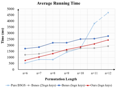
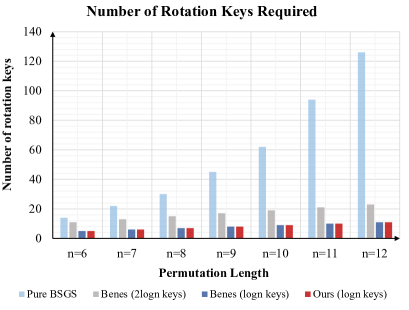
Figure 4: Performance of different implementation of arbitrary homomorphic vector permutation.

We know that various methods exist for implementing homomorphic vector permutation. To provide readers with a clear understanding of our proposed algorithm’s position, we further analyzed the performance of several typical homomorphic vector permutation algorithms, including their required number of rotation keys, as shown in Table 4. We selected four algorithms: the un-decomposed pure BSGS algorithm (with an inner-to-outer loop ratio not exceeding 2), a Benes network-based implementation with decomposition depth $\log{n}-1$ (split into two versions based on available rotation keys $\log{n}$ and $2\log{n}$), and our proposed algorithm.

From Figure 4, we can observe that, lacking decomposition, the pure BSGS algorithm’s permutation time escalates rapidly as $n$ increases, as does its required rotation key count. In contrast, permutation algorithms supported by decomposition exhibit a markedly slower growth in time and key requirements. Among these, the Benes network implementation needing $2\log{n}$ rotation keys is generally 40% to 50% faster than the $\log{n}$-key version. Our algorithm, however, achieves similar execution times to the $2\log{n}$-key Benes implementation while only requiring $\log{n}$ rotation keys. In summary, our approach provides a new trade-off for practical homomorphic permutation implementations, especially advantageous in scenarios where minimizing the number of rotation keys is essential.

7 Conclusion and further discussion

So far, we have discussed various aspects of homomorphic permutation. In Section 2 and Section 3, we defined an ideal form of homomorphic decomposition and constructed a depth-$1$ ideal decomposition search algorithm. In Section 4, using this search algorithm, we identified the full-depth decomposability of permutations in HMT and HMM. Finally, we proposed a new algorithm for computing arbitrary homomorphic permutations, converting permutations into multi-group network constructions that achieve better efficiency under minimal rotation key requirements, outperforming the current state-of-the-art Benes network-based approach.

However, there remain many unexplored aspects of homomorphic permutation. This includes: (i) categorizing permutations reducible to $U^{t}$ in terms of full-depth decomposability; (ii) designing level collapsing to our proposed multi-group network and integrating it with the BSGS algorithm and (iii) mitigating the complexity growth trend in its structure.

8 Acknowledgements

We extend our gratitude to all those who provided valuable insights and suggestions for this paper. Especially, we thank Jingru Tang for providing some initial ideas on this work.

References

- [1] Z. Brakerski and V. Vaikuntanathan, “Fully homomorphic encryption from ring-lwe and security for key dependent messages,” in Annual cryptology conference. Springer, 2011, pp. 505–524.
- [2] J. Fan and F. Vercauteren, “Somewhat practical fully homomorphic encryption,” Cryptology ePrint Archive, 2012.
- [3] J. H. Cheon, A. Kim, M. Kim, and Y. Song, “Homomorphic encryption for arithmetic of approximate numbers,” in Advances in Cryptology–ASIACRYPT 2017: 23rd International Conference on the Theory and Applications of Cryptology and Information Security, Hong Kong, China, December 3-7, 2017, Proceedings, Part I 23. Springer, 2017, pp. 409–437.
- [4] S. Halevi and V. Shoup, “Algorithms in helib,” in Advances in Cryptology–CRYPTO 2014: 34th Annual Cryptology Conference, Santa Barbara, CA, USA, August 17-21, 2014, Proceedings, Part I 34. Springer, 2014, pp. 554–571.
- [5] ——, “Faster homomorphic linear transformations in helib,” in Advances in Cryptology–CRYPTO 2018: 38th Annual International Cryptology Conference, Santa Barbara, CA, USA, August 19–23, 2018, Proceedings, Part I 38. Springer, 2018, pp. 93–120.
- [6] X. Jiang, M. Kim, K. Lauter, and Y. Song, “Secure outsourced matrix computation and application to neural networks,” in Proceedings of the 2018 ACM SIGSAC conference on computer and communications security, 2018, pp. 1209–1222.
- [7] J. H. Cheon, D. Kim, D. Kim, H. H. Lee, and K. Lee, “Numerical method for comparison on homomorphically encrypted numbers,” in International conference on the theory and application of cryptology and information security. Springer, 2019, pp. 415–445.
- [8] K. Han and D. Ki, “Better bootstrapping for approximate homomorphic encryption,” in Cryptographers’ Track at the RSA Conference. Springer, 2020, pp. 364–390.
- [9] J.-P. Bossuat, C. Mouchet, J. Troncoso-Pastoriza, and J.-P. Hubaux, “Efficient bootstrapping for approximate homomorphic encryption with non-sparse keys,” in Advances in Cryptology–EUROCRYPT 2021: 40th Annual International Conference on the Theory and Applications of Cryptographic Techniques, Zagreb, Croatia, October 17–21, 2021, Proceedings, Part I. Springer, 2021, pp. 587–617.
- [10] J.-W. Lee, E. Lee, Y. Lee, Y.-S. Kim, and J.-S. No, “High-precision bootstrapping of rns-ckks homomorphic encryption using optimal minimax polynomial approximation and inverse sine function,” in Advances in Cryptology–EUROCRYPT 2021: 40th Annual International Conference on the Theory and Applications of Cryptographic Techniques, Zagreb, Croatia, October 17–21, 2021, Proceedings, Part I 40. Springer, 2021, pp. 618–647.
- [11] S. Sav, A. Pyrgelis, J. R. Troncoso-Pastoriza, D. Froelicher, J.-P. Bossuat, J. S. Sousa, and J.-P. Hubaux, “Poseidon: Privacy-preserving federated neural network learning,” arXiv preprint arXiv:2009.00349, 2020.
- [12] J.-W. Lee, H. Kang, Y. Lee, W. Choi, J. Eom, M. Deryabin, E. Lee, J. Lee, D. Yoo, Y.-S. Kim et al., “Privacy-preserving machine learning with fully homomorphic encryption for deep neural network,” iEEE Access, vol. 10, pp. 30 039–30 054, 2022.
- [13] C. Gentry, S. Halevi, and N. P. Smart, “Fully homomorphic encryption with polylog overhead,” in Annual International Conference on the Theory and Applications of Cryptographic Techniques. Springer, 2012, pp. 465–482.
- [14] K. Han, M. Hhan, and J. H. Cheon, “Improved homomorphic discrete fourier transforms and fhe bootstrapping,” IEEE Access, vol. 7, pp. 57 361–57 370, 2019.
- [15] X. Ma, C. Ma, Y. Jiang, and C. Ge, “Improved privacy-preserving pca using optimized homomorphic matrix multiplication,” Computers & Security, vol. 138, p. 103658, 2024. [Online]. Available: https://www.sciencedirect.com/science/article/pii/S0167404823005679
- [16] P. Rizomiliotis and A. Triakosia, “On matrix multiplication with homomorphic encryption,” in Proceedings of the 2022 on Cloud Computing Security Workshop, 2022, pp. 53–61.
- [17] V. Lyubashevsky, C. Peikert, and O. Regev, “On ideal lattices and learning with errors over rings,” in Advances in Cryptology–EUROCRYPT 2010: 29th Annual International Conference on the Theory and Applications of Cryptographic Techniques, French Riviera, May 30–June 3, 2010. Proceedings 29. Springer, 2010, pp. 1–23.
- [18] ——, “A toolkit for ring-lwe cryptography,” in Annual international conference on the theory and applications of cryptographic techniques. Springer, 2013, pp. 35–54.
- [19] “Lattigo v4,” Online: https://github.com/tuneinsight/lattigo, Aug. 2022, ePFL-LDS, Tune Insight SA.
- [20] “Lattigo v5,” Online: https://github.com/tuneinsight/lattigo, Nov. 2023, ePFL-LDS, Tune Insight SA.
- [21] J.-P. Bossuat, R. Cammarota, J. H. Cheon, I. Chillotti, B. R. Curtis, W. Dai, H. Gong, E. Hales, D. Kim, B. Kumara et al., “Security guidelines for implementing homomorphic encryption,” Cryptology ePrint Archive, 2024.