Gnothi Seauton: Empowering Faithful Self-Interpretability in Black-Box Models

Abstract

The debate between self-interpretable models and post-hoc explanations for black-box models is central to Explainable AI (XAI). Self-interpretable models, such as concept-based networks, offer insights by connecting decisions to human-understandable concepts but often struggle with performance and scalability. Conversely, post-hoc methods like Shapley values, while theoretically robust, are computationally expensive and resource-intensive. To bridge the gap between these two lines of research, we propose a novel method that combines their strengths, providing theoretically guaranteed self-interpretability for black-box models without compromising prediction accuracy. Specifically, we introduce a parameter-efficient pipeline, AutoGnothi, which integrates a small side network into the black-box model, allowing it to generate Shapley value explanations without changing the original network parameters. This side-tuning approach significantly reduces memory, training, and inference costs, outperforming traditional parameter-efficient methods, where full fine-tuning serves as the optimal baseline. AutoGnothi enables the black-box model to predict and explain its predictions with minimal overhead. Extensive experiments show that AutoGnothi offers accurate explanations for both vision and language tasks, delivering superior computational efficiency with comparable interpretability.

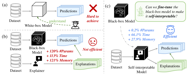
Figure 1: Different paradigms towards XAI. (a) The ideal paradigm for XAI envisions using white-box models for prediction, which are inherently self-interpretable by design but hard to achieve. (b) The previous paradigm involves post-hoc explanations of black-box models by training a separate, heavy-weight explainer. (c) We propose a novel parameter-efficient paradigm, AutoGnothi, which fine-tunes the black-box model to make it self-interpretable.

1 Introduction

Explainable AI (XAI) has gained increasing significance as AI systems are widely deployed in both vision (Dosovitskiy, 2020; Radford et al., 2021; Kirillov et al., 2023) and language domains (Devlin et al., 2019; Brown, 2020; Achiam et al., 2023). Ensuring interpretability in these systems is vital for fostering trust, ensuring fairness, and adhering to legal standards, particularly for complex models such as transformers. As illustrated in Figure 1(a), the ideal paradigm for XAI involves designing inherently transparent models that deliver superior performance. However, given the challenges in achieving this, current XAI methodologies can be broadly classified into two main categories: developing self-interpretable models and providing post-hoc explanations for black-box models.

Designing Self-Interpretable Models: Several notable efforts have focused on designing self-interpretable models that are grounded in solid mathematical foundations or learned concepts. Among these, concept-based networks have emerged as a representative approach linking model decisions to predefined, human-understandable concepts (Kim et al., 2018; Koh et al., 2020; Alvarez-Melis & Jaakkola, 2018). However, incorporating hand-crafted concepts often introduces a trade-off between interpretability and performance, as these models typically compromise the performance of the primary task. Moreover, such methods are often closely tied to specific architectures, which limits their scalability and transferability to other tasks. Furthermore, the explanations generated by concept-based models often lack a rigorous theoretical foundation, raising concerns about their reliability and overall trustworthiness.

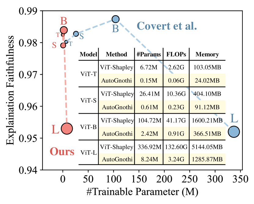
Figure 2: Explanation quality on the ImageNette dataset using different ViTs. Our AutoGnothi significantly reduces the number of trainable parameters, computational costs (FLOPs), and training GPU memory storage without compromising explanation quality.

Explaining Black-Box Models: Given the challenges of designing self-interpretable models for practical applications, post-hoc explanations for black-box models have become a widely adopted alternative. Among these, Shapley value-based methods (Shapley, 1953) are particularly valued for their theoretical rigor and adherence to four principled axioms (Young, 1985). However, calculating exact Shapley values involves evaluating all possible feature combinations, which scales exponentially with the number of features, making direct computation impractical for models with high-dimensional inputs. To alleviate this, methods like FastSHAP (Jethani et al., 2021) and ViT-Shapley (Covert et al., 2022) employ proxy explainers that estimate Shapley values during inference, significantly reducing the number of evaluations needed. While these approaches reduce some computational costs, training a separate explainer remains resource-intensive. For example, training a Vision Transformer (ViT) explainer requires more than twice the training GPU memory compared to the ViT classifier itself. Moreover, solely depending on post-hoc explanations for black-box models is not ideal in high-stakes decision-making scenarios, where immediate and reliable interpretability is required (Rudin, 2019).

To bridge the gap between existing methods and address the aforementioned challenges, the core objective of our research is to achieve theoretically guaranteed self-interpretability in advanced neural networks without sacrificing prediction performance, while minimizing training, memory, and inference costs. To this end, we propose a novel paradigm, AutoGnothi, which leverages parameter-efficient transfer learning (PETL) to substantially reduce the high training, memory, and inference costs associated with obtaining explainers. As depicted in Figure 3(a), traditional model-specific methods require two training stages: (i) fine-tuning a pre-trained model into a surrogate model, and (ii) training an explainer using the surrogate model. During inference, the original model is used for prediction, while a separate explainer network generates explanations, leading to two inference passes and double the storage overhead. In contrast, AutoGnothi utilizes side-tuning to reduce both training and memory costs, as shown in Figure 3(b). By incorporating an additive side branch parallel to the pre-trained model, we efficiently obtain a surrogate side network through side-tuning. We then apply the same strategy to develop the explainer side network, enabling simultaneous prediction and explanation in a single inference step. An illustrative example comparing the efficiency of AutoGnothi with previous methods is presented in Figure 2.

More importantly, AutoGnothi achieves self-interpretability without compromising prediction accuracy. Unlike a simple application of PETL, where full fine-tuning is considered the optimal baseline, our approach goes further. Experimental results show that relying on full fine-tuning to achieve self-interpretability often leads to degraded performance in either prediction or explanation tasks. In contrast, AutoGnothi maintains prediction accuracy while achieving self-interpretability by leveraging the intrinsic correlation between prediction and explanation. Beyond classical PETL, which primarily focuses on training efficiency, AutoGnothi also enhances inference efficiency through self-interpretation while keeping its faithfulness (see Section 4.2 for further discussion). Our key contributions are as follows:

1. Efficient Explanation: We introduce a novel PETL pipeline, AutoGnothi, which enables any black-box models, e.g., transformers, to become self-interpretable without affecting the original task parameters. By integrating and fine-tuning an additive side network, suprisingly surpasses previous methods in training, inference, and memory efficiency.

2. Self-interpretability: We achieve theoretically guaranteed self-interpretability for the black-box model with the Shapley value, without any influence on the original model’s prediction accuracy.

3. Broad Applications on both Vision and Language Models: We conducted experiments on the most widely used models, including ViT (Dosovitskiy, 2020) for image classification and BERT (Devlin et al., 2019) for sentimental analysis, showing that our methods outperform well on explanation quality. Specifically, for the ViT-base model pre-trained on ImageNette, our surrogates achieve a $97\%$ reduction in trainable parameters and $72\%$ reduction in training memory with comparable accuracy. For explainers, we achieve a $98\%$ reduction in trainable parameters, $77\%$ reduction in training memory. For generating explanation, AutoGnothi achieves $54\%$ reduction in inference computation, $44\%$ reduction in inference time, and a total parameter reduction of $54\%$.

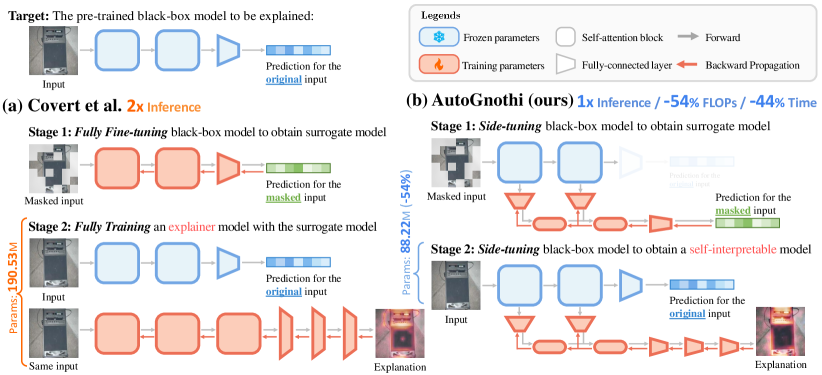
Figure 3: Overview of AutoGnothi compared to prior work. (a) ViT-Shapley (Covert et al., 2022) fully fine-tunes the black-box model to create a surrogate model, then trains a separate explainer based on the surrogate, which is resource-intensive. (b) We employ side-tuning to efficiently obtain both the black-box model and explainer, significantly reducing training costs. AutoGnothi uses a single model to simultaneously generate predictions and explanations, lowering inference costs by leveraging shared features. In contrast, ViT-Shapley needs to load two models for prediction and explanation, respectively, and infers two times. AutoGnothi enables self-interpretability for an arbitrary black-box model. We ignore the positional encoding associated with the pipeline.

2 Related work

Explaining Black-Box Models with Shapley Values: Among post-hoc explanation methods, the Shapley value (Shapley, 1953) is widely recognized as a faithful and theoretically sound metric for feature attribution, uniquely satisfying four key axioms: efficiency, symmetry, linearity, and dummy. However, computing Shapley values is computationally expensive, requiring $\mathcal{O}(2^{n})$ operations to calculate a single Shapley value for one feature in a set of size $n$. To alleviate this computational burden, various approaches have been proposed to expedite Shapley value computation, which can be broadly divided into model-agnostic and model-specific methods (Chen et al., 2023a). Model-agnostic techniques, such as KernelSHAP (Lundberg, 2017) and its enhancements (Covert & Lee, 2020), approximate Shapley values by sampling subsets of feature combinations. Nevertheless, when the feature set is large, the sampling cost remains prohibitive, and reducing this cost compromises the accuracy of the explanations, as fewer samples lead to less reliable estimates of feature importance. Conversely, model-specific methods, such as FastSHAP (Jethani et al., 2021) and ViT-Shapley (Covert et al., 2022), employ a trained proxy explainer to accelerate the estimation during inference, though these methods still involve significant training costs to develop the explainer.

Parameter Efficient Transfer Learning (PETL): PETL aims to achieve the performance of full fine-tuning while significantly reducing training costs by updating only a small subset of parameters. In this context, Adapters (Houlsby et al., 2019; Chen et al., 2023b) introduce trainable bottleneck modules into transformer layers, enabling models to deliver competitive results with minimal parameter adjustments. Another widely adopted method, LoRA (Hu et al., 2021), applies low-rank decomposition to the attention layer weights. Our work aligns more closely with side-tuning methods, where Side-Tuning (Zhang et al., 2020) integrates an auxiliary network that merges its representations with the backbone at the final layer, demonstrating effectiveness across diverse tasks in models like ResNet and BERT. LST (Sung et al., 2022) further improves this approach by reducing memory consumption through a ladder side network design. However, none of these methods explore the transfer of interpretability from the main model to the side network, leaving this a largely unexplored area in side-tuning and PETL research.

3 Background

3.1 Shapley Values

The Shapley value, originally introduced in game theory (Shapley, 1953), provides a method to fairly distribute rewards among players in coalitional games. In this framework, a set function assigns a value to any subset of players, corresponding to the reward earned by that subset. In machine learning scenarios, input variables are typically regarded as players, and a deep neural network (DNN) serves as the value function, assigning importance (saliency) to each input variable.

Let $s\in\{0,1\}^{d}$ be an indicator vector representing a specific variable subset for a sample $x=[x_{1},x_{2},\ldots,x_{d}]^{\top}\in\mathbb{R}^{d}$. Specifically, $x_{s}$ denotes the variables indicated by $s$, while those not in $s$ are replaced by a masked value (e.g., a baseline value). Let $e_{i}\in\mathbb{R}^{d}$ denote the vector with a one in the $i$-th position and zeros elsewhere. For a game involving $d$ players—or equivalently, a DNN $v:\{0,1\}^{d}\rightarrow\mathbb{R}$ with $d$ input variables—the Shapley values are denoted by $\phi_{v}(x_{1}),\ldots,\phi_{v}(x_{d})$. Each $\phi_{v}(x_{i})\in\mathbb{R}$ represents the value attributed to the $i$-th input variable $x_{i}$ in the sample $x$. The Shapley value $\phi_{v}(x_{i})$ is computed as follows:

$$\phi_{v}(x_{i})=\frac{1}{d}\sum_{s:s_{i}=0}\binom{d-1}{{\bm{1}}^{\top}s}\left(v(x_{s+e_{i}})-v(x_{s})\right).$$ (1)

Intuitively, Eq. (1) captures the average marginal contribution of the $i$-th player to the overall reward by considering all possible subsets in which player $i$ could be included. Shapley values satisfy four key axioms: linearity, dummy player, symmetry, and efficiency (Young, 1985). These axioms ensure a fair and consistent distribution of the total reward among all players.

3.2 Model-Based Estimation of Shapley Values

Calculating Shapley values to explain individual predictions presents substantial computational challenges (Chen et al., 2023a). To mitigate this burden, these values are typically approximated using sampling-based estimators, such as those in (Lundberg, 2017; Covert & Lee, 2020), though the sampling cost remains considerable. Recently, a more efficient model-based approach, introduced in (Jethani et al., 2021), accelerates the approximation by training a proxy explainer to compute Shapley values through a single model inference. However, this method has not been validated on advanced neural architectures such as transformers.

Building on this, ViT Shapley (Covert et al., 2022) was introduced to train a ViT explainer that interprets a pre-trained ViT model $f$. As shown in Figure 3(a), the learning process of the explainer consists of two stages. In stage 1, a surrogate model $g_{\beta}$ with parameters $\beta$ is generated by fine-tuning the pre-trained ViT classifier $f$ to handle partial information, which is used for calculating the masked variables in the Shapley value. This involves aligning the output distributions of the surrogate model $g_{\beta}$ with the classifier $f$. The surrogate is optimized with the following objective:

$$\mathcal{L}_{\textrm{surr}}(\beta)=\mathop{\mathbb{E}}_{\begin{subarray}{c}x\sim p(x),s\sim\mathcal{U}(0,d)\end{subarray}}\left[D_{\text{KL}}\left(f(x)\|g_{\beta}(x_{s})\right)\right],$$ (2)

where $\mathcal{U}(0,d)$ is a uniform distribution for sampling $s$. Then, in stage 2, an explainer $\phi_{\theta}$ with parameters $\theta$ is trained to generate explanations of the predictions of the black-box ViT $f$, utilizing the surrogate model $g_{\beta}$. This optimization method was first proposed by (Charnes et al., 1988) and later applied in (Lundberg, 2017; Jethani et al., 2021; Covert et al., 2022). Let $p(x)$ and $p(x,y)$ denote the distributions of input and input-label pairs, respectively. Specifically, the loss for training the explainer is:

$$\mathcal{L}_{\textrm{exp}}(\theta)= \mathop{\mathbb{E}}_{\begin{subarray}{c}(x,y)\sim p(x,y),s\sim q(s)\end{subarray}}\left[\left(g_{\beta}(x_{s}|y)-g_{\beta}(x_{{\bm{0}}}|y)-s^{\top}\phi_{\theta}(x,y)\right)^{2}\right]$$ (3)

$$\text{s.t.}\quad{\bm{1}}^{\top}\phi_{\theta}(x,y)=g_{\beta}(x_{{\bm{1}}}|y)-g_{\beta}(x_{{\bm{0}}}|y)\quad\forall(x,y),$$ (Efficiency)

where the constraint in the loss function is enforced to satisfy the efficiency axiom of the Shapley value, and $q(s)$ is defined with the Shapley kernel (Charnes et al., 1988) as follows:

$$q(s)\propto\frac{d-1}{\binom{d}{{\bm{1}}^{\top}s}({\bm{1}}^{\top}s)(d-{\bm{1}}^{\top}s)}\quad\forall s:0<{\bm{1}}^{\top}s<d,$$ (Shapley Kernel)

In addition, the ViT explainer $\phi_{\theta}$ has the same number of multi-head self-attention (MSA) layers as the feature backbone, and includes three additional MSA layers and a fully-connected (FC) layer as the explanation head. By learning the explainer $\phi_{\theta}$ to estimate Shapley values, the computational cost is reduced to a constant complexity of $\mathcal{O}(1)$.

4 Method

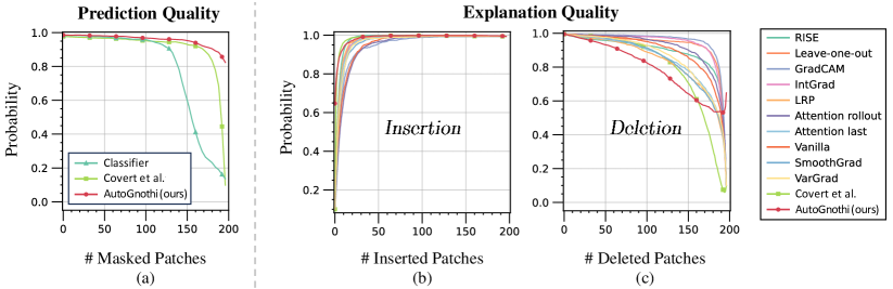
Figure 4: Training performance of surrogate and explainer models. (a) Prediction accuracy of masked inputs for the original classifier, the surrogate model trained with ViT Shapley (Covert et al., 2022), and our AutoGnothi. AutoGnothi shows greater robustness as the number of masked patches increases. For each mask size, we randomly sampled 100 images and generated 10 random masks. The curve represents the average prediction probability. (b) Explanation quality, measured by insertion and deletion metrics, for various explanation methods. We randomly sampled 1,000 images and averaged the prediction probabilities to assess insertion and deletion performance. All experiments were conducted on the ImageNette dataset using the ViT-base model.

4.1 Efficiently Training the Shapley Value Explainer for Black-Box Models

As discussed in Section 3.2, existing methods for approximating Shapley values require two stages. First, the black-box model $f$ is fully fine-tuned to obtain a surrogate model $g$ with the same trainable parameters and memory cost as $f$. Then, an explainer $\phi$ is fully trained using $g$. These stages at least double the training, memory, and inference costs compared to using the black-box model $f$ alone, making these methods impractical for large models.

To improve training, memory, and inference efficiency, we propose a side-tuning pipeline called AutoGnothi, as shown in Figure 3(b). Building on ideas PETL, we adapt Ladder Side-Tuning (LST) (Sung et al., 2022) by incorporating an additive side network. This side network separates the trainable parameters from the backbone model $f$ and adapts the model to a different task. It is a lightweight version of $f$, with weights and hidden state dimensions scaled by a factor of $1/r$, where $r$ is a reduction factor (e.g., $r=4$ or $8$). For instance, if the backbone $f$ has a $768$-dimensional hidden state, then with $r=8$, the side network has a hidden state dimension of $96$. By computing gradients solely for the side network, this design avoids a backward pass through the main backbone, improving training and memory efficiency. The formulation combines the frozen pre-trained backbone and the side-tuner with learnable parameters $\beta$ as:

$$y^{\text{main}}=\underbrace{f}_{\text{frozen}}(x),\quad y^{\text{surr}}=\underbrace{g_{\beta}}_{\text{trainable}}(x_{s}),\quad{\phi}^{\text{exp}}=\underbrace{\phi_{\theta}}_{\text{trainable}}(x),$$ (4)

where $g_{\beta}$ is trained by minimizing the loss in Eq.(2), and $\phi_{\theta}$ is trained by minimizing the loss in Eq.(3), respectively.

Table 1: Comparison of training and memory efficiency across different models. We evaluated memory consumption and trainable parameters for previous methods (Covert et al., 2022) and AutoGnothi across a range of models and tasks. For surrogate models, we measured classification accuracy, while for explainers, we assessed explanation quality using insertion and deletion metrics. It is important to note that prediction accuracy for the classifier is evaluated on normal inputs, whereas for the surrogate model, accuracy is measured on masked inputs.

Dataset		ImageNette				MURA	Pet	Yelp
Model		ViT-T	ViT-S	ViT-B	ViT-L	ViT-B	ViT-B	BERT-B
Classifier to be explained	Memory (MB)	84.90	331.80	1311.61	4631.25	1311.50	1311.93	1676.59
	#Params (M)	5.53	21.67	85.81	303.31	85.80	85.83	109.48
	Accuracy (↑)	0.9791	0.9944	0.9944	0.9964	0.8186	0.9469	0.9010
Surrogate (Covert et al.)	Memory (MB)	84.90	331.80	1311.61	4631.25	1311.50	1311.93	1676.59
	#Params (M)	5.53	21.67	85.81	303.31	85.80	85.83	109.48
	Accuracy (↑)	0.9822	0.9934	0.9939	0.9975	0.8233	0.9469	0.9490
Surrogate (AutoGnothi)	Memory (MB)	23.83 (-72%)	92.38 (-72%)	363.64 (-72%)	1280.80 (-72%)	438.10 (-67%)	363.76 (-72%)	532.71 (-68%)
	#Params (M)	0.14 (-97%)	0.56 (-97%)	2.23 (-97%)	7.91 (-97%)	7.11 (-92%)	2.23 (-97%)	7.15 (-93%)
	Accuracy (↑)	0.9791	0.9939	0.9959	0.9959	0.8139	0.9422	0.9280
Explainer (Covert et al.)	Memory (MB)	103.05	404.10	1600.21	5144.05	1599.79	1601.47	1955.87
	#Params (M)	6.72	26.41	104.72	336.92	104.69	104.80	127.79
	Insertion (↑)	0.9824	0.9828	0.9839	0.9843	0.9319	0.9422	0.9620
	Deletion (↓)	0.5243	0.6865	0.8121	0.7646	0.4199	0.4958	0.1725
Explainer (AutoGnothi)	Memory (MB)	24.02 (-77%)	93.12 (-77%)	366.51 (-77%)	1285.87 (-75%)	449.38 (-72%)	366.75 (-77%)	685.32 (-65%)
	#Params (M)	0.15 (-98%)	0.61 (-98%)	2.42 (-98%)	8.24 (-98%)	7.85 (-93%)	2.43 (-98%)	17.15 (-87%)
	Insertion (↑)	0.9802	0.9791	0.9874	0.9837	0.9292	0.9384	0.9588
	Deletion (↓)	0.5097	0.6667	0.7954	0.6570	0.4116	0.4888	0.1004

4.1.1 Obtaining the Surrogate

To obtain the surrogate model, AutoGnothi applies LST directly to the black-box model $f$, utilizing the additive side branch $g$ with parameters $\beta$ to predict the masked inputs $x_{s}$ of sample $x$. Let $f^{(i)}$ and $g^{(i)}$ denote the $i$-th MSA block of the main model $f$ and the surrogate branch $g$, respectively. Assume there are $N$ MSA blocks in total. Let $z_{1}^{\text{main}}$ denote the output for masked input $x_{s}$ of the first MSA layer $f^{(1)}$ of $f$, i.e., $z_{1}^{\text{main}}=f^{(1)}(x_{s})$. The forward process of the frozen main model $f$ with the side-tuning branch $g$ is:

$$z_{i}^{\text{main}}=f^{(i)}(z_{i-1}^{\text{main}}),\quad z_{i}^{\text{surr}}=g^{(i)}(\text{FC}^{(i)}(z_{i}^{\text{main}})).$$ (5)

After $N$ MSA blocks, an FC head is applied to generate the prediction for the partial information, i.e., $y^{\text{surr}}=\text{FC}_{\text{head}}(z_{N}^{\text{surr}}))$. The convergence of the surrogate model is analyzed as follows:

Theorem 1 (Proof in Appendix B).

Let the surrogate model be trained using gradient descent with step size $\alpha$ for $t$ iterations. The expected KL divergence between the original model’s predictions $f(x)$ and the surrogate model’s predictions $g_{\beta}(x_{s})$ is upper-bounded by:

$$\mathbb{E}_{x\sim p(x),s\sim\mathcal{U}(0,d)}\left[D_{\text{KL}}\left(f(x)\|g_{\beta}(x_{s})\right)\right]\leq\frac{1}{2\mu}(1-\mu\alpha)^{t}\left(\mathcal{L}_{\text{surr}}(\beta_{0})-\mathcal{L}_{\text{surr}}^{\star}\right),$$ (6)

where $\beta_{0}$ is the initial parameter value, $\mathcal{L}_{\text{surr}}^{\star}$ is the optimal value during optimization, and $\mu$ is the minimal eigenvalue of the Hessian of $\mathcal{L}_{\text{surr}}$.

Theorem 1 establishes a theoretical guarantee that a side-tuned surrogate can achieve performance comparable to that of a fully trained surrogate. The detailed proof is provided in Appendix B.

Figure 3(b) shows the pipeline of obtaining the surrogate in stage 1. An intuitive performance comparison of prediction models is presented in Figure 4(a). AutoGnothi’s surrogate surpasses the original classifier in terms of prediction accuracy and matches the performance of (Covert et al., 2022) when handling partial information, but with only $3\%$ trainable parameters. Additionally, AutoGnothi’s surrogate exhibits more robust predictions as the number of masked inputs increases. A detailed comparison of the training and memory costs on different models is provided in Table 1.

4.1.2 Obtaining the Explainer

For the explainer model, AutoGnothi uses a similar LST feature backbone as in the surrogate model $g$, consisting of $N$ MSA blocks for feature extraction. Let $\phi^{(i)}$ represent the $i$-th MSA block of the explainer branch $\phi$. In addition to the lightweight backbone blocks in the side branch, we add $M$ extra FC layers as the explanation head. Together, the side network $\phi$ generates explanations based on the backbone features from the main branch. Let $z_{1}^{\text{main}}$ denote the output for input $x$ from the first MSA layer $f^{(i)}$ of the main branch $f$, i.e., $z_{1}^{\text{main}}=f^{(1)}(x)$. The forward process of the explainer is:

$$z_{i}^{\text{main}}=f^{(i)}(z_{i-1}^{\text{main}}),\quad z_{i}^{\text{exp}}=\phi^{(i)}(\text{FC}^{(i)}(z_{i}^{\text{main}}))\quad\forall i\in\{1,\ldots,N\},$$ (7)

$${\phi}^{\text{exp}}(x)=\text{FC}_{\text{head}}^{(M)}\left(\text{FC}_{\text{head}}^{(M-1)}\left(\ldots\left(\text{FC}_{\text{head}}^{(1)}\left(z_{N}^{\text{exp}}\right)\right)\right)\right),$$

where the main branch $f$ remains uncontaminated. We provide a theoretical guarantee for the convergence of the trained side branch $\phi$ as follows:

Theorem 2 (Proof in Appendix B).

Let $\phi_{v}(x|y)$ denote the exact Shapley value for input-output pair $(x,y)$ in game $v$. The expected regression loss $\mathcal{L}_{\text{exp}}(\theta)$ upper bounds the Shapley value estimation error as follows,

$$\mathbb{E}_{p(x,y)}\Big{[}\big{|}\big{|}\phi_{\theta}(x,y)-\phi_{v}(x|y))\big{|}\big{|}_{2}\Big{]}\leq\sqrt{2H_{d-1}\Big{(}\mathcal{L}_{\text{exp}}(\theta)-\mathcal{L}^{\star}_{\text{exp}}\Big{)}},$$ (8)

where $\mathcal{L}^{\star}_{\text{exp}}$ represents the optimal loss achieved by the exact Shapley values, and $H_{d-1}$ is the $(d-1)$-th harmonic number.

Theorem 2 provides a theoretical guarantee that a side-tuned explainer can achieve performance on par with a fully trained explainer. The complete proof is presented in Appendix B.

Figure 3(b) shows the pipeline of obtaining the explainer in stage 2. We evaluated the explanation quality of AutoGnothi against various baselines, as shown in Figure 4(b). AutoGnothi achieved the highest insertion and lowest deletion scores among $12$ explanation methods, demonstrating superior explanation quality. Compared to (Covert et al., 2022), we reduced the trainable parameters for explainers by $98\%$ while maintaining comparable or even superior interpretability. Table 1 provides detailed comparisons of training and memory efficiency for different models.

Table 2: Inference efficiency comparison of various models. We assessed the computational cost (FLOPs), total parameters, and inference time for different methods. For the baseline method (Covert et al., 2022), we calculated these values separately for the classifier and explainer, and then combined them. In contrast, for AutoGnothi, we computed these values directly from our self-interpretable models, who can generate both predictions and explanations simultaneously.

Dataset		ImageNette				MURA	Pet	Yelp
Model		ViT-T	ViT-S	ViT-B	ViT-L	ViT-B	ViT-B	BERT-B
Classifier + Explainer (Covert et al.)	FLOPs (G)	4.78	18.86	74.90	251.96	74.88	74.93	213.51
	Time (ms)	19.7	39.0	94.9	310.3	100.3	100.2	166.90
	#Params (M)	12.25	48.08	190.53	640.23	190.49	190.63	237.27
Self-Interpretable Model (AutoGnothi)	FLOPs (G)	2.22 (-54%)	8.73 (-54%)	34.67 (-54%)	122.60 (-51%)	36.81 (-51%)	34.67 (-54%)	116.66 (-45%)
	a Time (ms)	15.4 (-22%)	23.0 (-41%)	52.9 (-44%)	179.1 (-42%)	56.7 (-43%)	57.0 (-43%)	118.55 (-29%)
	#Params (M)	5.68 (-54%)	22.28 (-54%)	88.22 (-54%)	311.55 (-51%)	93.65 (-51%)	88.25 (-54%)	126.63 (-47%)

4.1.3 Generating Explanation for Black-Box Models

After obtaining the explainer, we now detail the explanation procedure. In most post-hoc explanation methods (Selvaraju et al., 2020; Chattopadhay et al., 2018; Binder et al., 2016; Covert et al., 2022), predictions and explanations must be computed separately for a single input. For instance, as illustrated in Figure 3(a), two separate inferences are required to explain a single prediction. In contrast, as shown in Figure 3(b), AutoGnothi generates both predictions and explanations simultaneously, needing only one inference. To evaluate this efficiency, we measured inference time, computational cost (FLOPs), and total parameters required to generate predictions and explanations for different methods. The comparison of inference efficiency is highlighted in Table 2.

4.2 Difference between AutoGnothi and previous PETL Methods

In this section, we provide an empirical analysis of why AutoGnothi outperforms previous PETL approaches. We highlight that AutoGnothi is not a simple extension of classical PETL, where full fine-tuning is typically the optimal baseline. Additionally, AutoGnothi exploits the intrinsic correlation between the prediction task and its explanation, enabling black-box models to become self-interpretable without sacrificing prediction accuracy. We elaborate on these two points below.

Full fine-tuning poses challenges for achieving self-interpretability and is not the optimal baseline for AutoGnothi. For classical PETL, the goal is often to match the performance of fully fine-tuned models on standard tasks (Houlsby et al., 2019; Chen et al., 2023b; Hu et al., 2021; Mercea et al., 2024). However, in XAI scenarios, the challenge shifts: it becomes difficult, if not impossible, to train a model that balances both prediction accuracy and explanation quality (Arrieta et al., 2020; Gunning et al., 2019; Došilović et al., 2018). In fact, fine-tuning models to adapt interpretability without forgetting pre-trained knowledge can be difficult (Li & Hoiem, 2017). Additionally, full fine-tuning the original model also puts us in the Theseus’s Paradox: we won’t be sure if we are explaining the very same model anymore. Even if full fine-tuning were practical, it would contradict the goal of interpreting the pre-trained model. In contrast, AutoGnothi pipeline addresses this issue by freezing the primary model and training only a side network to generate explanations, offering an efficient solution that enables self-interpretability without degrading prediction performance.

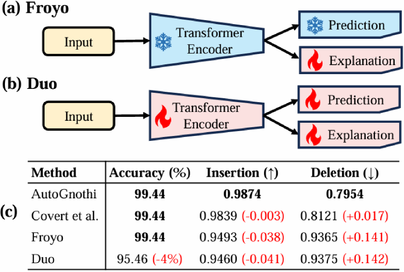
Figure 5: Other pipelines to achieve the self-interpretability through the full fine-tuning. (a) Freeze the transformer encoder and prediction head, learning only the explanation head. (b) Simultaneously learn the transformer encoder, and both task heads. (c) Comparison of classification and explanation performance between different pipelines for ViT-base.

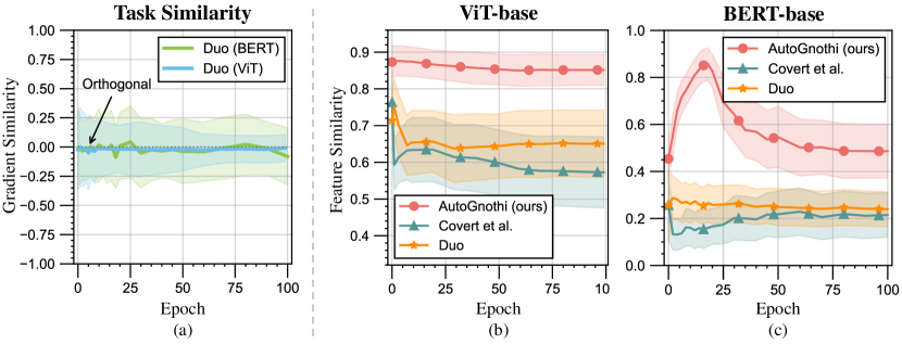
Figure 6: Explanation of why the Duo pipeline underperforms compared to AutoGnothi. (a) The full fine-tuning strategy employed by Duo is not the optimal baseline for AutoGnothi due to significant gradient conflicts between the prediction and explanation tasks. This conflict results in degraded performance, raising concerns about whether the explanation truly pertains to the same model. Note that gradient similarity can only be measured for the Duo pipeline, as other methods freeze the prediction backbones. (b) In contrast, AutoGnothi exhibits a stronger correlation between features of the prediction and explanation tasks. We measured the feature similarity with CKA.

Building on prior work that highlights the challenges of achieving self-interpretability through full fine-tuning, we conducted experiments to further explore this issue. As depicted in Figure 6(a)(b), we introduce two additional pipelines, Froyo and Duo. Froyo adds an explanation head while keeping the transformer encoder and prediction head frozen to preserve prediction accuracy. In contrast, Duo jointly learns both the prediction task and its explanation. Both pipelines use the same encoder, prediction head, and explanation head architectures as described in (Covert et al., 2022).

We performed experiments using ViT-base model trained on the ImageNette dataset. Our findings show that the Froyo pipeline underperforms due to the limited trainable parameters in the explanation head, resulting in degraded explanation quality. As illustrated in Figure 6(c), this led to a reduction in insertion by $0.038$ and an increase in deletion by $0.141$, despite no impact on prediction accuracy.

For the Duo pipeline, we observed a $4.0\%$ decline in prediction accuracy on the ViT-base model, accompanied by a reduction in insertion by $0.041$ and an increase in deletion by $0.142$. Further empirical evidence, as depicted in Figure 6(a), highlights conflicting gradients between the prediction and explanation tasks during training. Additionally, as previously discussed, the Theseus’s Paradox arises when changes in predictions result in evolving explanations, thereby challenging the consistency and identity of the original model.

AutoGnothi uncovers the intrinsic correlation between predictions and explanations. While the AutoGnothi pipeline enables self-interpretation with superior efficiency, the underlying mechanisms connecting prediction and explanation remain underexplored. We propose that AutoGnothi leverages the intrinsic relationship between the backbone features used for both tasks. This correlation is illustrated in Figure 6(b), where we evaluated the Central Kernel Alignment (CKA) (Kornblith et al., 2019) between the backbone features of the original pre-trained model and those of various explainers. Our results show that AutoGnothi exhibits higher feature similarity between prediction and explanation tasks on ViT-base and BERT-base models, supporting our hypothesis.

5 Experiments

5.1 Experimental Settings

Datasets and Black-box Models. For image classification, we used the ImageNette (Howard & Gugger, 2020), Oxford IIIT-Pets (Parkhi et al., 2012), and MURA (Rajpurkar et al., 2017) datasets, following (Covert et al., 2022). For sentiment analysis, we utilized the Yelp Review Polarity dataset (Zhang et al., 2015). In terms of black-box models, we employed the widely used ViT models (Dosovitskiy, 2020) for vision tasks, including ViT-tiny, ViT-small, ViT-base, and ViT-large. For language tasks, we used the BERT-base model (Devlin et al., 2019).

Table 3: Quality metrics (insertion and deletion) for target class explanations of ViT-base across baseline methods and AutoGnothi on the ImageNette dataset. More results for other datasets and models are provided in Appendix C.

Method	Insertion (↑)	Deletion (↓)
Random	0.9578$\pm$0.0790	0.9584$\pm$0.0764
Attention last	0.9633$\pm$0.0659	0.8524$\pm$0.1748
Attention rollout	0.9408$\pm$0.0834	0.9168$\pm$0.1277
GradCAM (Attn)	0.9447$\pm$0.0936	0.9562$\pm$0.0916
GradCAM (LN)	0.9343$\pm$0.0829	0.9426$\pm$0.1307
Vanilla (Pixel)	0.9487$\pm$0.0688	0.8945$\pm$0.1513
Vanilla (Embed)	0.9563$\pm$0.0643	0.8618$\pm$0.1754
IntGrad (Pixel)	0.9670$\pm$0.0575	0.9408$\pm$0.1141
IntGrad (Embed)	0.9670$\pm$0.0575	0.9408$\pm$0.1141
SmoothGrad (Pixel)	0.9591$\pm$0.0760	0.8459$\pm$0.1788
SmoothGrad (Embed)	0.9529$\pm$0.0931	0.9561$\pm$0.0764
VarGrad (Pixel)	0.9616$\pm$0.0725	0.8600$\pm$0.1692
VarGrad (Embed)	0.9552$\pm$0.0901	0.9568$\pm$0.0756
LRP	0.9677$\pm$0.0623	0.8393$\pm$0.1866
Leave-one-out	0.9696$\pm$0.0353	0.9334$\pm$0.1493
RISE	0.9772$\pm$0.0225	0.8959$\pm$0.1962
Covert et al.	0.9839$\pm$0.0375	0.8121$\pm$0.1768
AutoGnothi (Ours)	0.9874$\pm$0.0265	0.7954$\pm$0.2294

Implementation Details. For surrogates and explainers, AutoGnothi incorporates the same number of MSA blocks as the black-box model being explained in the side network and utilizes a reduction factor of $r=8$ for the lightweight side branch on both the ImageNette and Oxford IIIT-Pets datasets, and $r=4$ for MURA and Yelp Review Polarity. Surrogates use the same task head as the black-box classifiers with one additional FC layer as classification head for handling partial information. Explainers utilize three additional FC layers as the explanation head after the side network backbone. For attention masking, we employed a causal attention masking strategy, setting attention values to a large negative number before applying the softmax operation (Brown, 2020). More detailed training settings are provided in Appendix A.

Evaluation Metrics for Explanations. We used the widely adopted insertion and deletion metrics (Petsiuk, 2018) to evaluate explanation quality. These metrics are computed by progressively inserting or deleting features based on their importance and observing the impact on the model’s predictions. The corresponding surrogate model trained to handle partial inputs is used for this process to generate prediction for masked inputs. We calculated the area under the curve (AUC) for the predictions and average results for randomly selected $1,000$ samples on all datasets.

Baseline Methods. We considered $12$ representative explanation methods for comparison. For attention-based methods, we utilized attention rollout and attention last (Abnar & Zuidema, 2020). For gradient-based methods, we used Vanilla Gradients (Simonyan, 2013), IntGrad (Sundararajan et al., 2017), SmoothGrad (Smilkov et al., 2017), VarGrad (Hooker et al., 2019), LRP (Binder et al., 2016), and GradCAM (Selvaraju et al., 2020). For removal-based methods, we employed leave-one-out (Zeiler & Fergus, 2014) and RISE (Petsiuk, 2018). For Shapley value-based methods, we utilized KernelSHAP (Lundberg, 2017) and ViT Shapley (Covert et al., 2022) as baselines.

5.2 Evaluating Training, Memory and Inference Efficiency

To evaluate the training and memory efficiency of AutoGnothi, we compared it with various baselines in terms of trainable parameters and memory usage. Table 1 provides a summary of the memory costs and trainable parameters for both surrogate and explainer models across different methods. During training, AutoGnothi achieves a significant reduction of over $87\%$ in trainable parameters and more than $65\%$ in GPU memory usage for both surrogates and explainers on both vision and language datasets, while maintaining competitive performance in both prediction accuracy and explanation quality. The memory cost is evaluated with training batch size $=1$.

Next, we evaluate the inference efficiency of our self-interpretable models by comparing the computational cost (FLOPs), inference time, and the total number of parameters required for generating both predictions and explanations. As shown in Table 2, AutoGnothi significantly reduces inference time and FLOPs compared to baseline models that require separate inferences for predictions and explanations. Specifically, when both the predictions and the explanations are required, AutoGnothi is capable of reducing at least $45\%$ in FLOPs, $22\%$ in inference time (up to $44\%$), and $47\%$ in total parameters end-to-end across all datasets and tasks.

5.3 Evaluating Explanation Quality

Quantitative Results. To evaluate the quality of explanations generated by AutoGnothi, we compared it against $12$ state-of-the-art baseline methods using the insertion and deletion metrics. Table 3 presents results from a ViT-base model trained on the ImageNette dataset, where AutoGnothi consistently achieves the best insertion and deletion scores for target class explanations across various datasets. Further detailed results for other models and tasks are provided in Appendix C. For vision task, please refer to Tables 4, 5, and 6 for the results of ViT-tiny, ViT-small, and ViT-large on ImageNette, respectively. Results for ViT-base on Oxford-IIIT Pets are provided in Table 7, and results for ViT-base on Mura are shown in Table 8. For language task, we also provide results of BERT-base on Yelp Reivew Polarity in Table 9.

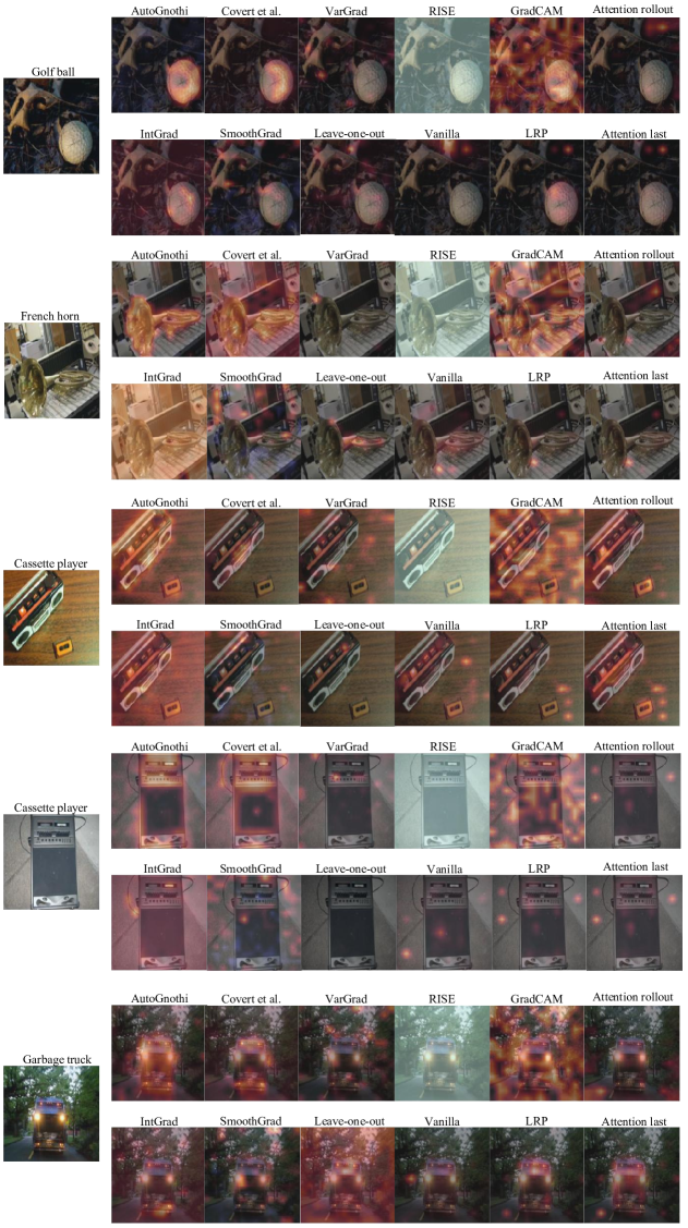
Figure 8: Visualization of ViT-base explanation on ImageNette dataset (1/2).

Qualitative Results. We also provide visualization results for ViTs on different datasets, as shown in Figure 7. It may be observed that RISE happened to fail to provide human-interpretable or intuitive results, which amongst all others AutoGnothi offers more accurate explanations with a clearer focus on the subject and diluted colours for irrelevant classes. Additional visualization results for ViT-base on more datasets are provided in Appendix D, shown in Figures 8, 9, 10, 11, 12, and 13.

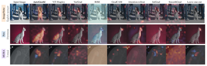
Figure 7: Visualization of ViT explanations on the ImageNette, Oxford-IIIT Pets, and MURA datasets. AutoGnothi qualitatively outperforms other baseline approaches.

6 Conclusion

This paper introduces AutoGnothi to bridge the gap between self-interpretable models and post-hoc explanation methods in Explainable AI. Inspired by parameter-efficient transfer-learning, AutoGnothi incorporates a lightweight side network that allows black-box models to generate faithful Shapley value explanations without affecting the original predictions. Notably, AutoGnothi outperforms directly finetuning the all the parameters in the model for explanation by a clear margin. This approach empowers black-box models with self-interpretability, which is superior to standard post-hoc explanations that require generating predictions and explanations in two separate, heavy inferences. Experiments on ViT and BERT demonstrate that AutoGnothi achieves superior efficiency on computation, storage and memory in both training and inference periods.

Appendix A Further Experimental Details

A.1 Environment

Our experiments were conducted on one 128-core AMD EPYC 9754 CPU with one NVIDIA GeForce RTX 4090 GPU with 24 GB VRAM. No multi-card training or inference was involved. We implemented the training and inference pipelines for image classification tasks under the PyTorch Lightning framework, and for the sentiment analysis task with just PyTorch. For evaluations on baseline methods we leverage the SHAP library (Lundberg, 2017), with minor modifications applied to bridge data format differences between Numpy and PyTorch.

A.2 FLOPs and Memory

We used the profile function from the thop library to evaluate the FLOPs for each model during the inference stage. Memory consumption was manually calculated during the training stage based on the model parameters, activations, and intermediate results. Our memory estimations were made under the assumption that the memory was evaluated under a batch size of $1$ and uses 32-bit floating point precision (torch.float32).

A.3 Classifier

The training of all tasks is split into 3 stages. In the first stage parameters of the classifier are inherited from the original base model verbatim, with the exception of AutoGnothi adding additional parameters for the new side branch, initialized with Kaiming initialization.

We fine-tune this classifier model on the exact same dataset with the AdamW optimizer, using a learning rate of $10^{-5}$ for $25$ epochs, and retain the best checkpoint rated by minimal validation loss. Classification loss is minimum square error with respective to the predicted classes and the ground-truth labels. For AutoGnothi the classes come from the side branch, while all remaining models use the classes from the main branch. We train and evaluate these methods on 1 Nvidia RTX 4090, and use a batch size of $32$ samples provided that it fits inside the available GPU memory.

We freeze parameters in all stages likewise. As is described in 4.2, AutoGnothi only trains the side branch and all parameters from the original model are frozen. In ViT-shapley (Covert et al.) and Duo pipelines, all parameters are trained, whilst the Froyo pipeline only trains the classification head.

A.4 Surrogate

Surrogate models have the same model architecture as the classifiers, with a different recipe. We load all parameters from the classifier without any changes or additions, further fine-tune the model for $50$ epochs, and retain the best checkpoint with minimal validation loss.

Unlike the classifier, the surrogate model focuses on mimicking the classifier model’s behavior under a masked context. Consider the logits $p(y|x_{\bm{0}})$ from the classifier model, where $x$ is the input and $y$ is the corresponding class label. The surrogate model aims at closing in its masked logits distribution, $p(y|x_{s})$, with the original distribution:

$$\mathcal{L}_{\text{surr}}(\beta)=\mathop{\mathbb{E}}_{\begin{subarray}{c}x\sim p(x),s\sim\mathcal{U}(0,d)\end{subarray}}\left[D_{\text{KL}}\left(f(x)\|g_{\beta}(x_{s})\right)\right],$$ (1)

The mask is selected on an equi-categorical basis. We first pick an integer $n_{s}=s\cdot{\bm{1}}^{\top}$ at uniform distribution, denoting the number of tokens that shall be masked. $n_{s}$ mutually exclusive indices are then randomly chosen from the input at uniform distribution. To avoid inhibiting model capabilities, special tokens like the implicit class token in ViT or the [CLS] token applied by the BERT tokenizer are never masked.

In order to selectively hide or mask inputs from the model, we apply causal attention masks for both the image models and text models in our experiments. However, it’s worth noting that while they may confuse the transformer’s attention mechanisms, certain other methods are also capable of concealing these input tokens, primarily zeroing or assigning random values to the said pixels in image models, or assigning [PAD] and [MASK] to the selected tokens. We follow prior work (Covert et al., 2022) and adhere to causal attention masks.

Recall that the transformer self-attention mechanism used in ViT (Dosovitskiy, 2020), BERT (Devlin et al., 2019). Given an attention input $t\in\mathbb{R}^{d\times h}$ and self-attention parameters $W_{\textrm{qkv}}\in\mathbb{R}^{h\times 3h^{\prime}}$, whereas $d$ is the number of tokens and $h$ is the attention’s hidden size, and $h^{\prime}$ be the size of each attention head, the output of the self-attention $\textrm{SA}(t)$ for a single head is computed as follows:

$$\left[Q,K,V\right] =u\cdot W_{\textrm{qkv}}$$ (2)

$$A =\textrm{softmax}\left(\frac{Q\cdot K^{\top}}{\sqrt{h^{\prime}}}\right)$$ (3)

$$\textrm{SA}(t) =A\cdot V$$ (4)

Transformers in practice use a multiple $k$ attention heads, holding that $k\cdot h^{\prime}=h$. An attention projection matrix $P_{\textrm{msa}}\in\mathbb{R}^{h\times h}$ is used to combine the outputs of all attention heads. Denoting the $i$-th self-attention head’s output as $SA_{i}(t)$, the final output of the attention layer $\textrm{MSA}(t)$ is thus computed:

$$\textrm{MSA}(t)=\left[\textrm{SA}_{1}(t),\textrm{SA}_{2}(t),\ldots,\textrm{SA}_{n}(t)\right]\cdot P_{\textrm{msa}}$$ (5)

We notice that the attention mechanism is entirely unrelated to the number of tokens, and can operate in the absence of certain input tokens. Let an indicator vector $s\in\{0,1\}^{d}$ correspond to a subset of the input tokens (applying equally to images and text tokens), we calculate the masked self-attention over $t$ and $s$ as follows:

$$\left[Q,K,V\right] =u\cdot W_{Q,K,V}$$ (6)

$$A =\textrm{softmax}\left(\frac{Q\cdot K^{\top}-(1-s)\cdot\infty}{\sqrt{h^{\prime}}}\right)$$ (7)

$$\textrm{SA}(t,s) =A\cdot V$$ (8)

We apply masking to the multi-head attention layers likewise, such that:

$$\textrm{MSA}(t,s)=\left[\textrm{SA}_{1}(t,s),\textrm{SA}_{2}(t,s),\ldots,\textrm{SA}_{n}(t,s)\right]\cdot P_{\textrm{msa}}$$ (9)

This mechanism is widely implemented for attention models in commonplace libraries such as HuggingFace’s Transformers, named by the argument attention_mask in the input tensor.

A.5 Explainer

We load explainer model parameters from surrogate model checkpoints, such that all are copied from the surrogate model to the explainer model, except for the last classification head, which is replaced with an explainer head. The explainer head contains 3 MLP layers and a final linear layer, with GeLU (Hendrycks & Gimpel, 2017) activations from in between. For AutoGnothi only the classification head on the side branch is replaced. We train the explainer model for $100$ epochs with the AdamW optimizer, using a learning rate of $10^{-5}$, and keep the best checkpoint.

In our implementation, we took 2 input images in each mini-batch and generated $16$ random masks for each image, resulting in a parallelism of 32 instances per batch. A slight change is applied to the masking algorithm in the explainer model from the surrogate model, in order to reduce variance during gradient descent. Specifically, in addition to generating masks uniform, we follow prior work (Covert et al., 2022) and use the paired sampling trick (Covert & Lee, 2020), pairing each subset $s$ with its complement ${\bm{1}}-s$. This algorithm equally applies to both image and text classification models.

The explainer model is trained to approximate the Shapley value $\phi_{\theta}(x,y)$. Let $g_{\beta}(x_{s}|y)$ be the surrogate values respective to the input $x$ and the class $y$, masked by the indicator vector $s$, and $g_{\beta}(x_{\bm{0}}|y)$ be the surrogate values without masking. Following (Covert et al., 2022), we minimize the following loss function:

$$\mathcal{L}_{exp}(\theta)= \mathop{\mathbb{E}}_{\begin{subarray}{c}(x,y)\sim p(x,y),s\sim q(s)\end{subarray}}\left[\left(g_{\beta}(x_{s}|y)-g_{\beta}(x_{{\bm{0}}}|y)-s^{\top}\phi_{\theta}(x,y)\right)^{2}\right]$$ (10)

$$\text{s.t.}\quad{\bm{1}}^{\top}\phi_{\theta}(x,y)=g_{\beta}(x_{{\bm{1}}}|y)-g_{\beta}(x_{{\bm{0}}}|y)\quad\forall(x,y),$$ (Efficiency)

Notice that the explainer model $\phi_{\theta}(x,y)$ is being trained under a mean squared error loss, and that $16$ random masks are generated for each image in the mini-batch. The explainer is hence optimized against a distribution of the Shapley values, so an accurate calculation of ground-truth Shapley values for each training sample is not even remotely necessary.

Also, the aforementioned efficiency constraint is necessary for the explainer model to output faithful and exact Shapley values. We leverage additive efficient normalization from (Ruiz et al., 1998) and use the same approach as prior work (Jethani et al., 2021; Covert et al., 2022) to enforce this constraint. The model is trained to make unconstrained predictions as is described in equation 10, which we then modify using the following transformation to have it constrained:

$$\phi_{\theta}(x,y)\leftarrow\phi_{\theta}(x,y)+\frac{g_{\beta}(x_{\bm{1}}|y)-g_{\beta}(x_{\bm{0}}|y)-{\bm{1}}^{T}\cdot\phi_{\theta}(x,y)}{d}$$ (11)

After training the explainer model, we merge the original classifier model and all relevant intermediate stages’ models into one single, independent model to contain both the classification task and the explanation task to have them run concurrently. For the baseline method, ViT-shapley and its modified counterpart for NLP, no parameters overlap between the two tasks, thus inference must be done on both tasks resulting in a huge implied performance overhead. AutoGnothi, however, only requires a validation pass to ensure that the original classifier head is preserved verbatim in the final model. This is done by comparing the output of the original classifier and the final model on any arbitrary input.

A.6 Datasets

In this section we explain in more detail which datasets are selected and how they are processed for our experiments. Three datasets are used for the image classification task. The ImageNette dataset includes $9,469$ training samples and $3,925$ validation samples for $10$ classes. MURA (musculoskeletal radiographs) has $36,808$ training samples and $3,197$ validation samples for $2$ classes. The Oxford-IIIT Pets dataset contains $5,879$ training samples, $735$ validation samples and $735$ test samples in $37$ classes. For the text classification (sequence classification) task, we use the Yelp Polarity dataset, which originally contains $560,000$ training samples and $38,000$ test samples.

For each epoch, image classifiers (ViT) iterate through all available images in either of the train or test dataset. Specifically to during training, images are normalized by the mean value and standard deviation of each corresponding training dataset, before being down-sampled to $224\times 224$ pixels. For text classifiers, each of the epoch is trained on exactly $2048$ training samples randomly chosen from the dataset, and validated on $256$ equally random test samples. This is primarily done to serve our needs in frequent checkpoints for more thorough data analysis such as on CKA or parameter gradients.

Due to the sheer cost from some metrics on certain tasks, we reduced the size of our test set during evaluation. We selected $1000$ test samples for datasets ImageNette, MURA and Yelp Review Polarity, and randomly selected $300$ samples for the Oxford-IIIT Pets dataset. For each dataset this subset stays the same between different explanation methods and different model sizes. We emphasize that these samples are deliberately independent from the training set to avoid potential bias from the results.

Appendix B Proofs of Theorems

Here we provide detailed proof for Theorem 1 and Theorem 2, which provide theoretical guarantee for the performance of surrogates and explainers. Our proof follows (Simon & Vincent, 2020) and (Covert et al., 2022), which exhibit similar results for a single data point.

Lemma 1.

For a single input $x$, the expected loss under Eq. (2) is $\mu$-strongly convex, where $\mu$ is the minimal eigenvalue of the Hessian of $\mathcal{L}_{\textrm{surr}}(\beta)$.

Proof.

The expected loss for a single input $x$ under the new objective function is given by:

$$\mathcal{L}_{\textrm{surr}}(\beta)=\mathbb{E}_{s\sim\mathcal{U}(0,d)}\left[D_{\text{KL}}(f(x)\|g_{\beta}(x_{s}))\right].$$ (12)

This loss function is convex in $\beta$ because the KL divergence $D_{\text{KL}}(f(x)\|g_{\beta}(x_{s}))$ is convex in $g_{\beta}(x_{s})$, and $g_{\beta}(x_{s})$ is a smooth function of $\beta$. The Hessian of $\mathcal{L}_{\textrm{surr}}(\beta)$ with respect to $\beta$ is:

$$\nabla^{2}_{\beta}\mathcal{L}_{\textrm{surr}}(\beta)=\mathbb{E}_{s\sim\mathcal{U}(0,d)}\left[\nabla^{2}_{\beta}D_{\text{KL}}(f(x)\|g_{\beta}(x_{s}))\right].$$ (13)

The convexity of $\mathcal{L}_{\textrm{surr}}(\beta)$ is determined by the smallest eigenvalue of this Hessian, $\mu$. Since the KL divergence is strictly convex, the minimum eigenvalue is positive, which implies $\mu$-strong convexity. ∎

Theorem 1.

Let the surrogate model be trained using gradient descent with step size $\alpha$ for $t$ iterations. The expected KL divergence between the original model’s predictions $f(x)$ and the surrogate model’s predictions $g_{\beta}(x_{s})$ is upper-bounded by:

$$\mathbb{E}_{x\sim p(x),s\sim\mathcal{U}(0,d)}\left[D_{\text{KL}}\left(f(x)\|g_{\beta}(x_{s})\right)\right]\leq\frac{1}{2\mu}(1-\mu\alpha)^{t}\left(\mathcal{L}_{\textrm{surr}}(\beta_{0})-\mathcal{L}_{\textrm{surr}}^{\star}\right),$$ (14)

where $\beta_{0}$ is the initial parameter value, and $\mathcal{L}_{\textrm{surr}}^{\star}$ is the optimal value during optimization.

Proof.

Let the surrogate model be trained using gradient descent with step size $\alpha$ for $t$ iterations. The optimization process for minimizing the expected KL divergence between $f(x)$ and $g_{\beta}(x_{s})$ can be written as:

$$\beta_{t+1}=\beta_{t}-\alpha\nabla_{\beta}\mathcal{L}_{\textrm{surr}}(\beta_{t}).$$ (15)

Because $\mathcal{L}_{\textrm{surr}}(\beta)$ is $\mu$-strongly convex, we can apply the standard result for gradient descent convergence on strongly convex functions, which gives the following bound:

$$\mathcal{L}_{\textrm{surr}}(\beta_{t})-\mathcal{L}_{\textrm{surr}}^{\star}\leq(1-\mu\alpha)^{t}\left(\mathcal{L}_{\textrm{surr}}(\beta_{0})-\mathcal{L}_{\textrm{surr}}^{\star}\right),$$ (16)

where $\mathcal{L}_{\textrm{surr}}^{\star}$ is the optimal value, and $\beta_{0}$ is the initial parameter value.

Since the KL divergence is bounded by the expected loss, we have:

$$\mathbb{E}_{x\sim p(x),s\sim\mathcal{U}(0,d)}\left[D_{\text{KL}}(f(x)\|g_{\beta}(x_{s}))\right]\leq\mathcal{L}_{\textrm{surr}}(\beta_{t}).$$ (17)

Substituting the bound on $\mathcal{L}_{\textrm{surr}}(\beta_{t})$, we obtain:

$$\mathbb{E}_{x\sim p(x),s\sim\mathcal{U}(0,d)}\left[D_{\text{KL}}(f(x)\|g_{\beta}(x_{s}))\right]\leq\frac{1}{2\mu}(1-\mu\alpha)^{t}\left(\mathcal{L}_{\textrm{surr}}(\beta_{0})-\mathcal{L}_{\textrm{surr}}^{\star}\right).$$ (18)

∎

Lemma 2.

For a single input-output pair $(x,y)$, the expected loss under Eq.(3) for the prediction $\phi_{\theta}(x,y)$ is $\mu$-strongly convex with $\mu=H_{d-1}^{-1}$, where $H_{d-1}$ is the $(d-1)$-th harmonic number.

Proof.

For an input-output pair $(x,y)$, the expected loss for the prediction $\phi=\phi_{\theta}(x,y)$ is defined as

$$L_{\theta}(x,y) =\mathbb{E}_{s\sim p(s)}\Big{[}\big{(}g_{\beta}(x_{s}|y)-g_{\beta}(x_{{\bm{0}}}|y)-s^{\top}\phi\big{)}^{2}\Big{]}$$ (19)

$$=\phi^{\top}\mathbb{E}_{s\sim p(s)}[ss^{\top}]\phi-2\mathbb{E}_{s\sim p(s)}\Big{[}s\big{(}g_{\beta}(x_{s}|y)-g_{\beta}(x_{{\bm{0}}}|y)\big{)}\Big{]}\phi$$

$$+\mathbb{E}_{s\sim p(s)}\Big{[}\big{(}g_{\beta}(x_{s}|y)-g_{\beta}(x_{{\bm{0}}}|y)\big{)}^{2}\Big{]}.$$

This is a quadratic function of $\phi$ with its Hessian given by

$$\nabla_{\theta}^{2}L_{\theta}(x,y)=2\cdot\mathbb{E}_{s\sim p(s)}[ss^{\top}].$$ (20)

The eigenvalues of the Hessian determine the convexity of $L_{\theta}(x,y)$, and the entries of the Hessian can be derived from the subset distribution $p(s)$. The distribution assigns equal probability to subsets with the same cardinality, thus we define the shorthand $p_{k}\equiv p(s)$ for $s$ such that ${\bm{1}}^{\top}s=k$. Specifically, we have:

$$p_{k}=Q^{-1}\frac{d-1}{\binom{d}{k}k(d-k)}\quad\quad\text{and}\quad\quad Q=\sum_{k=1}^{d-1}\frac{d-1}{k(d-k)}.$$ (21)

We can then write $A\equiv\mathbb{E}_{s\sim p(s)}[ss^{\top}]$ and derive its entries as follows:

$$A_{ii} =\Pr(s_{i}=1)=\sum_{k=1}^{d}\binom{d-1}{k-1}p_{k}$$ (22)

$$=Q^{-1}\sum_{k=1}^{d-1}\frac{d-1}{d(d-k)}$$

$$=\frac{\sum_{k=1}^{d-1}\frac{d-1}{d(d-k)}}{\sum_{k=1}^{d-1}\frac{d-1}{k(d-k)}}$$

$$A_{ij} =\Pr(s_{i}=s_{j}=1)=\sum_{k=2}^{d}\binom{d-2}{k-2}p_{k}$$ (23)

$$=Q^{-1}\sum_{k=2}^{d-1}\frac{k-1}{d(d-k)}$$

$$=\frac{\sum_{k=2}^{d-1}\frac{k-1}{d(d-k)}}{\sum_{k=1}^{d-1}\frac{d-1}{k(d-k)}}.$$

Based on this, we observe that $A$ has the structure $A=(b-c)I_{d}+c{\bm{1}}{\bm{1}}^{\top}$, where $b\equiv A_{ii}-A_{ij}$ and $c\equiv A_{ij}$. Following (Simon & Vincent, 2020; Covert et al., 2022), the minimum eigenvalue is given by $\lambda_{\min}(A)=b-c$. A more detailed derivation reveals that it depends on the $(d-1)$-th harmonic number, $H_{d-1}$:

$$\lambda_{\mathrm{min}}(A) =b-c=A_{ii}-A_{ij}$$ (24)

$$=\frac{\sum_{k=1}^{d-1}\frac{d-1}{d(d-k)}}{\sum_{k=1}^{d-1}\frac{d-1}{k(d-k)}}-\frac{\sum_{k=2}^{d-1}\frac{k-1}{d(d-k)}}{\sum_{k=1}^{d-1}\frac{d-1}{k(d-k)}}$$

$$=\frac{\frac{1}{d}+\sum_{k=2}^{d-1}\frac{d-k}{d(d-k)}}{\sum_{k=1}^{d-1}\frac{d-1}{k(d-k)}}$$

$$=\frac{\frac{1}{d}+\frac{d-2}{d}}{\sum_{k=1}^{d-1}\frac{d-1}{k(d-k)}}$$

$$=\frac{d-1}{d}\cdot\frac{1}{\sum_{k=1}^{d-1}\frac{d-1}{k(d-k)}}$$

$$=\frac{1}{2\sum_{k=1}^{d-1}\frac{1}{k}}$$

$$=\frac{1}{2H_{d-1}}.$$

The minimum eigenvalue is therefore strictly positive, implying that $L_{\theta}(x,y)$ is $\mu$-strongly convex, where $\mu$ is given by

$$\mu =2\cdot\lambda_{\mathrm{min}}(A)=H_{d-1}^{-1}.$$ (25)

Note that the strong convexity constant $\mu$ is independent of $(x,y)$ and is determined solely by the number of input variables $d$. ∎

Theorem 2.

Let $\phi_{v}(x|y)$ denote the exact Shapley value for input-output pair $(x,y)$ in game $v$. The expected regression loss $\mathcal{L}_{\textrm{exp}}(\theta)$ upper bounds the Shapley value estimation error as follows,

$$\mathbb{E}_{(x,y)\sim p(x,y)}\Big{[}\big{|}\big{|}\phi_{\theta}(x,y)-\phi_{v}(x|y))\big{|}\big{|}_{2}\Big{]}\leq\sqrt{2H_{d-1}\Big{(}\mathcal{L}_{\textrm{exp}}(\theta)-\mathcal{L}^{\star}_{\textrm{exp}}\Big{)}},$$ (26)

where $\mathcal{L}^{\star}_{\textrm{exp}}$ represents the optimal loss achieved by the exact Shapley values.

Proof.

We begin by considering a single input-output pair $(x,y)$, where the prediction is given by $\phi=\phi_{\theta}(x,y;\theta)$. To account for the linear constraint (the Shapley value’s efficiency constraint) in our objective, we write the Lagrangian $L_{\theta}(x,y,\gamma)$:

$$L_{\theta}(x,y,\gamma)=L_{\theta}(x,y)+\gamma\left(g_{\beta}(x_{\mathbf{1}}|y)-g_{\beta}(x_{\mathbf{0}}|y)-\mathbf{1}^{\top}\phi\right),$$ (27)

where $\gamma\in\mathbb{R}$ is the Lagrange multiplier. The Lagrangian $L_{\theta}(x,y,\gamma)$ is $\mu$-strongly convex, sharing the same Hessian as $L_{\theta}(x,y)$:

$$\nabla_{\theta}^{2}L_{\theta}(x,y,\gamma)=\nabla_{\theta}^{2}L_{\theta}(x,y).$$ (28)

By strong convexity, we can bound the distance between $\phi$ and the global minimizer using the Lagrangian’s value. Let $(\theta^{\star},\gamma^{\star})$ be the optimizer of the Lagrangian, such that

$$\phi_{\theta^{\star}}(x,y)=\phi_{v}(x|y),$$ (29)

where $\phi_{v}(x|y)$ is the exact Shapley value.

From the first-order condition of strong convexity, we obtain the inequality:

$$L_{\theta}(x,y,\gamma^{\star})\geq L_{\theta^{\star}}(x,y,\gamma^{\star})+(\phi-\phi_{\theta^{\star}}(x,y))^{\top}\nabla_{\theta}L_{\theta^{\star}}(x,y,\gamma^{\star})+\frac{\mu}{2}\|\phi-\phi_{\theta^{\star}}(x,y)\|^{2}_{2}.$$ (30)

By the KKT conditions, $\nabla_{\theta}L_{\theta^{\star}}(x,y,\gamma^{\star})=0$, so the inequality simplifies to:

$$L_{\theta}(x,y,\gamma^{\star})\geq L_{\theta^{\star}}(x,y,\gamma^{\star})+\frac{\mu}{2}\|\phi-\phi_{\theta^{\star}}(x,y)\|^{2}_{2}.$$ (31)

Rearranging this, we get:

$$\|\phi-\phi_{\theta^{\star}}(x,y)\|^{2}_{2}\leq\frac{2}{\mu}\left(L_{\theta}(x,y,\gamma^{\star})-L_{\theta^{\star}}(x,y,\gamma^{\star})\right).$$ (32)

Since $\phi$ is a feasible solution (i.e., it satisfies the linear constraint), this further simplifies to:

$$\|\phi-\phi_{\theta^{\star}}(x,y)\|^{2}_{2}\leq\frac{2}{\mu}\left(L_{\theta}(x,y)-L_{\theta^{\star}}(x,y)\right).$$ (33)

Next, we take the expectation over $(x,y)\sim p(x,y)$. Denote the expected regression loss as $\mathcal{L}_{exp}(\theta)$, which is:

$$\mathcal{L}_{\textrm{exp}}(\theta)=\mathbb{E}_{(x,y)\sim p(x,y)}\left[\big{(}g_{\beta}(x_{s}|y)-g_{\beta}(x_{\mathbf{0}}|y)-s^{\top}\phi_{\theta}(x,y;\theta)\big{)}^{2}\right].$$ (34)

Let $\mathcal{L}_{\textrm{exp}}^{\star}$ denote the loss achieved by the exact Shapley values. Taking the bound from the previous inequality in expectation, we have:

$$\mathbb{E}_{(x,y)\sim p(x,y)}\left[\|\phi_{\theta}(x,y;\theta)-\phi_{v}(x|y)\|^{2}_{2}\right]\leq\frac{2}{\mu}\left(\mathcal{L}_{\textrm{exp}}(\theta)-\mathcal{L}_{\textrm{exp}}^{\star}\right).$$ (35)

Finally, applying Jensen’s inequality to the left-hand side, we obtain:

$$\mathbb{E}_{(x,y)\sim p(x,y)}\left[\|\phi_{\theta}(x,y;\theta)-\phi_{v}(x|y)\|_{2}\right]\leq\sqrt{\frac{2}{\mu}\left(\mathcal{L}_{\textrm{exp}}(\theta)-\mathcal{L}_{\textrm{exp}}^{\star}\right)}.$$ (36)

Substituting the value of $\mu=1/H_{d-1}$ from Lemma 2, we conclude that:

$$\mathbb{E}_{(x,y)\sim p(x,y)}\left[\|\phi_{\theta}(x,y;\theta)-\phi_{v}(x|y)\|_{2}\right]\leq\sqrt{2H_{d-1}\left(\mathcal{L}_{\textrm{exp}}(\theta)-\mathcal{L}_{\textrm{exp}}^{\star}\right)}.$$ (37)

∎

Appendix C Additional Results for AutoGnothi

In addition to the results on ImageNette included in the main paper, we provide more detailed results on other datasets ranging from image classification tasks to text classification tasks, against a number of baseline explanation methods, with respect to other model sizes in this section.

Table 4: Performance metrics for ViT-tiny on ImageNette.

Method	Insertion (↑)	Deletion (↓)
Random	0.9231$\pm$0.1094	0.9229$\pm$0.1106
Attention last	0.9281$\pm$0.1033	0.7311$\pm$0.2422
Attention rollout	0.9138$\pm$0.1102	0.7306$\pm$0.2449
GradCAM (Attn)	0.9155$\pm$0.1242	0.8292$\pm$0.2089
GradCAM (LN)	0.9280$\pm$0.0937	0.8436$\pm$0.2046
Vanilla (Pixel)	0.9006$\pm$0.1173	0.8161$\pm$0.2034
Vanilla (Embed)	0.9131$\pm$0.1109	0.7708$\pm$0.2272
IntGrad (Pixel)	0.9383$\pm$0.0808	0.8734$\pm$0.1817
IntGrad (Embed)	0.9317$\pm$0.0808	0.8092$\pm$0.1817
SmoothGrad (Pixel)	0.9153$\pm$0.1199	0.7724$\pm$0.2236
SmoothGrad (Embed)	0.9268$\pm$0.1092	0.7852$\pm$0.2176
VarGrad (Pixel)	0.9219$\pm$0.1147	0.7872$\pm$0.2157
VarGrad (Embed)	0.9317$\pm$0.1063	0.8092$\pm$0.2062
LRP	0.9439$\pm$0.0852	0.6883$\pm$0.2603
Leave-one-out	0.9632$\pm$0.0401	0.7671$\pm$0.2902
RISE	0.9743$\pm$0.0333	0.6514$\pm$0.3028
Covert et al.	0.9824$\pm$0.0289	0.5243$\pm$0.2579
AutoGnothi (Ours)	0.9802$\pm$0.0268	0.5097$\pm$0.2688

Table 5: Performance metrics for ViT-small on ImageNette.

Method	Insertion (↑)	Deletion (↓)
Random	0.9471$\pm$0.0827	0.9461$\pm$0.0843
Attention last	0.9599$\pm$0.0771	0.7617$\pm$0.2205
Attention rollout	0.9293$\pm$0.0940	0.8566$\pm$0.1793
GradCAM (Attn)	0.9217$\pm$0.1205	0.9301$\pm$0.1186
GradCAM (LN)	0.9239$\pm$0.0893	0.9184$\pm$0.1571
Vanilla (Pixel)	0.9535$\pm$0.1006	0.8179$\pm$0.1686
Vanilla (Embed)	0.9564$\pm$0.0894	0.8240$\pm$0.1886
IntGrad (Pixel)	0.9581$\pm$0.0738	0.9219$\pm$0.1281
IntGrad (Embed)	0.9581$\pm$0.0738	0.9219$\pm$0.1281
SmoothGrad (Pixel)	0.9542$\pm$0.0770	0.7998$\pm$0.2055
SmoothGrad (Embed)	0.9550$\pm$0.0788	0.8065$\pm$0.2090
VarGrad (Pixel)	0.9535$\pm$0.0798	0.8179$\pm$0.1954
VarGrad (Embed)	0.9564$\pm$0.0776	0.8240$\pm$0.1942
LRP	0.9636$\pm$0.0637	0.7549$\pm$0.2275
Leave-one-out	0.9684$\pm$0.0319	0.8815$\pm$0.2056
RISE	0.9773$\pm$0.0206	0.7960$\pm$0.2599
Covert et al.	0.9828$\pm$0.0440	0.6865$\pm$0.2255
AutoGnothi (Ours)	0.9791$\pm$0.0305	0.6667$\pm$0.2636

Table 6: Performance metrics for ViT-large on ImageNette.

Method	Insertion (↑)	Deletion (↓)
Random	0.9645$\pm$0.0748	0.9642$\pm$0.0757
Attention last	0.9251$\pm$0.0794	0.8997$\pm$0.1380
Attention rollout	0.9336$\pm$0.0835	0.9429$\pm$0.0997
GradCAM (Attn)	0.9398$\pm$0.0692	0.9328$\pm$0.1228
GradCAM (LN)	0.9590$\pm$0.0619	0.9366$\pm$0.1330
Vanilla (Pixel)	0.9040$\pm$0.1046	0.9372$\pm$0.1106
Vanilla (Embed)	0.9151$\pm$0.0959	0.9258$\pm$0.1237
IntGrad (Pixel)	0.9716$\pm$0.0584	0.9596$\pm$0.0948
IntGrad (Embed)	0.9716$\pm$0.0584	0.9596$\pm$0.0948
SmoothGrad (Pixel)	0.9499$\pm$0.0778	0.8953$\pm$0.1579
SmoothGrad (Embed)	0.9636$\pm$0.0681	0.8664$\pm$0.1643
VarGrad (Pixel)	0.9444$\pm$0.0827	0.9060$\pm$0.1456
VarGrad (Embed)	0.9558$\pm$0.0687	0.8827$\pm$0.1545
LRP	0.9506$\pm$0.0646	0.8814$\pm$0.1530
Leave-one-out	0.9743$\pm$0.0521	0.9534$\pm$0.1085
RISE	0.9801$\pm$0.0373	0.9245$\pm$0.1570
Covert et al.	0.9843$\pm$0.0436	0.7646$\pm$0.2012
AutoGnothi (Ours)	0.9837$\pm$0.0225	0.6570$\pm$0.2171

Table 7: Performance metrics for ViT-base on Oxford-IIIT Pet.

Method	Insertion (↑)	Deletion (↓)
Random	0.8642$\pm$0.1855	0.8625$\pm$0.1851
Attention last	0.9066$\pm$0.1302	0.5534$\pm$0.2183
Attention rollout	0.8616$\pm$0.1384	0.7387$\pm$0.2326
GradCAM (Attn)	0.8726$\pm$0.1585	0.7582$\pm$0.2296
GradCAM (LN)	0.8828$\pm$0.1137	0.7648$\pm$0.2462
Vanilla (Pixel)	0.8855$\pm$0.1362	0.6551$\pm$0.2395
Vanilla (Embed)	0.8996$\pm$0.1354	0.5783$\pm$0.2405
IntGrad (Pixel)	0.9219$\pm$0.1137	0.8451$\pm$0.1990
IntGrad (Embed)	0.9219$\pm$0.1137	0.8451$\pm$0.1990
SmoothGrad (Pixel)	0.9140$\pm$0.1329	0.5508$\pm$0.2347
SmoothGrad (Embed)	0.8731$\pm$0.1462	0.8716$\pm$0.1514
VarGrad (Pixel)	0.9145$\pm$0.1268	0.5801$\pm$0.2366
VarGrad (Embed)	0.8818$\pm$0.1437	0.8778$\pm$0.1487
LRP	0.9192$\pm$0.1178	0.5362$\pm$0.2258
Leave-one-out	0.9468$\pm$0.0666	0.7341$\pm$0.2951
RISE	0.9581$\pm$0.0333	0.6186$\pm$0.3096
Covert et al.	0.9422$\pm$0.1035	0.4958$\pm$0.2404
AutoGnothi (Ours)	0.9384$\pm$0.1088	0.4888$\pm$0.2480

Table 8: Performance metrics for ViT-base on MURA. MURA is a binary classification dataset, we calculate metrics for each of its two categories.

	Abnormal		Normal
Method	Insertion (↑)	Deletion (↓)	Insertion (↑)	Deletion (↓)
Random	0.8195$\pm$0.1875	0.8206$\pm$0.1859	0.1548$\pm$0.1396	0.1564$\pm$0.1415
Attention last	0.8416$\pm$0.1863	0.6303$\pm$0.1912	0.1546$\pm$0.1365	0.1849$\pm$0.1348
Attention rollout	0.8047$\pm$0.1887	0.7236$\pm$0.2107	0.1758$\pm$0.1393	0.1636$\pm$0.1366
GradCAM (Attn)	0.8077$\pm$0.1883	0.8172$\pm$0.1925	0.1611$\pm$0.1387	0.1655$\pm$0.1518
GradCAM (LN)	0.8509$\pm$0.1787	0.7451$\pm$0.2171	0.1771$\pm$0.1537	0.1487$\pm$0.1338
Vanilla (Pixel)	0.8384$\pm$0.1764	0.5971$\pm$0.2056	0.1710$\pm$0.1401	0.1603$\pm$0.1310
Vanilla (Embed)	0.8412$\pm$0.1774	0.5709$\pm$0.1993	0.1666$\pm$0.1393	0.1649$\pm$0.1295
IntGrad (Pixel)	0.8677$\pm$0.1642	0.7690$\pm$0.2261	0.2011$\pm$0.1842	0.1326$\pm$0.1283
IntGrad (Embed)	0.8677$\pm$0.1642	0.7690$\pm$0.2261	0.2011$\pm$0.1842	0.1326$\pm$0.1283
SmoothGrad (Pixel)	0.8351$\pm$0.1893	0.6469$\pm$0.2000	0.1610$\pm$0.1428	0.1842$\pm$0.1385
SmoothGrad (Embed)	0.8293$\pm$0.1863	0.8006$\pm$0.1971	0.1605$\pm$0.1500	0.1552$\pm$0.1406
VarGrad (Pixel)	0.8397$\pm$0.1844	0.6667$\pm$0.2012	0.1592$\pm$0.1404	0.1813$\pm$0.1453
VarGrad (Embed)	0.8328$\pm$0.1841	0.8022$\pm$0.1983	0.1575$\pm$0.1461	0.1556$\pm$0.1418
LRP	0.8524$\pm$0.1786	0.6009$\pm$0.1932	0.1693$\pm$0.1459	0.1745$\pm$0.1238
Leave-one-out	0.8996$\pm$0.1336	0.6887$\pm$0.2412	0.2952$\pm$0.2235	0.0977$\pm$0.0911
RISE	0.9247$\pm$0.1037	0.6258$\pm$0.2510	0.3470$\pm$0.2431	0.0844$\pm$0.0786
Covert et al.	0.9319$\pm$0.0795	0.4199$\pm$0.2136	0.4516$\pm$0.2506	0.0539$\pm$0.0478
AutoGnothi (Ours)	0.9292$\pm$0.0597	0.4116$\pm$0.2116	0.4563$\pm$0.2524	0.0581$\pm$0.0488

Table 9: Performance metrics for Bert-base on Yelp Review Polarity.

Method	Insertion (↑)	Deletion (↓)
KernelShap	0.8894$\pm$0.1324	0.4624$\pm$0.2548
Covert et al.	0.9620$\pm$0.0472	0.1725$\pm$0.1176
AutoGnothi (Ours)	0.9588$\pm$0.0206	0.1004$\pm$0.0377

Appendix D Additional Visualizations for AutoGnothi

In this section we present a number of image samples on the ViT-base model, regarding explanation outputs from 12 representative baseline explanation methods. We ensure that these samples correspond to correct model predictions made by the base model to ensure better clarity.

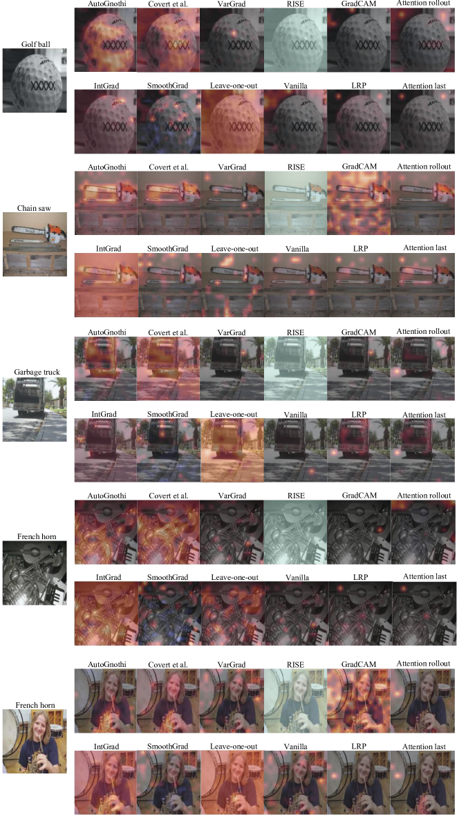
Figure 9: Visualization of ViT-base explanation on ImageNette dataset (2/2).

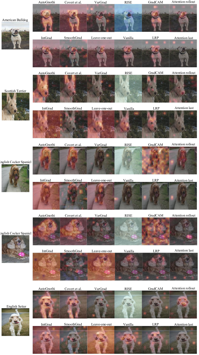
Figure 10: Visualization of ViT-base explanation on Oxford-IIIT Pet dataset (1/2).

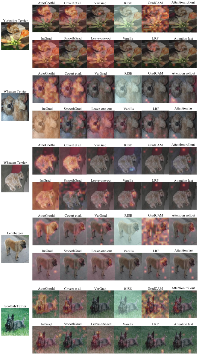
Figure 11: Visualization of ViT-base explanation on Oxford-IIIT Pet dataset (2/2).

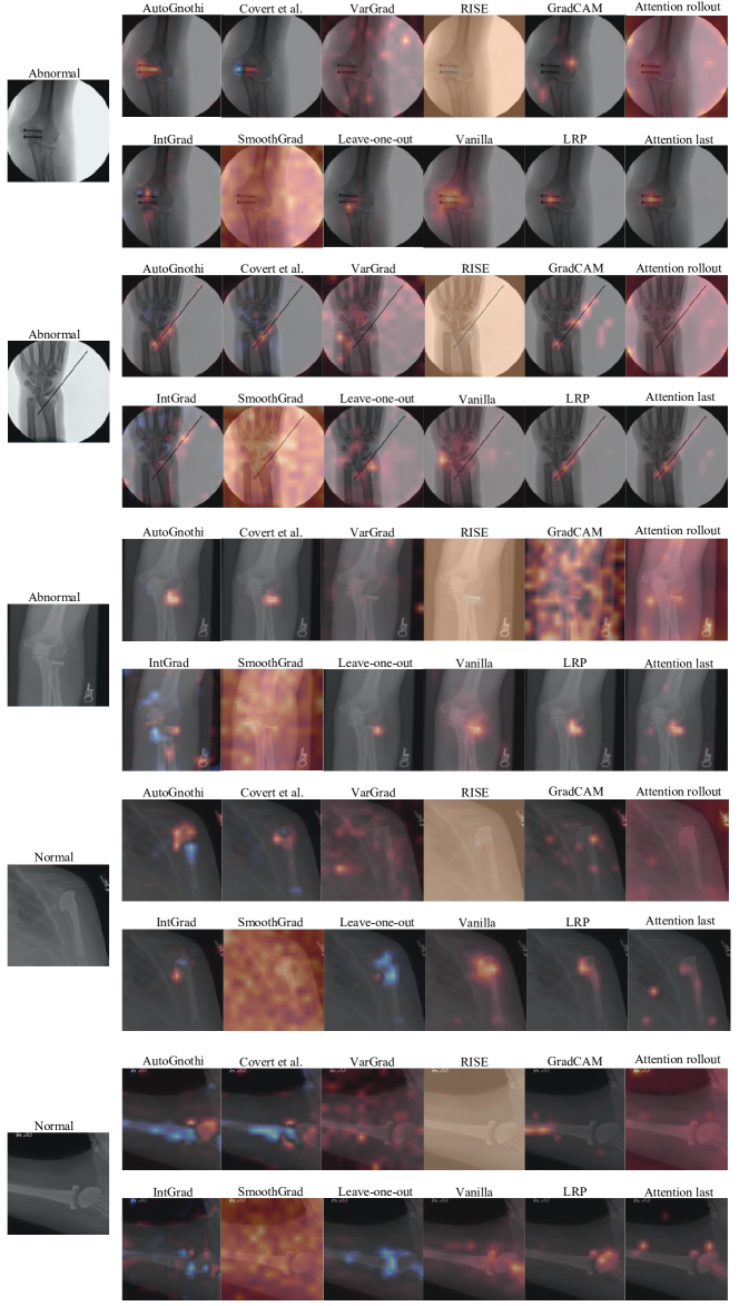
Figure 12: Visualization of ViT-base explanation on MURA dataset (1/2).

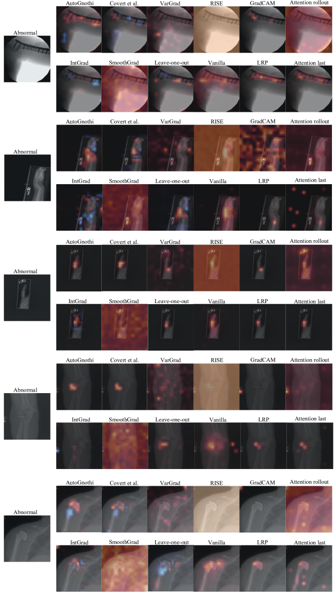
Figure 13: Visualization of ViT-base explanation on MURA dataset (2/2).

References

- Abnar & Zuidema (2020) Samira Abnar and Willem Zuidema. Quantifying attention flow in transformers. In Proceedings of the 58th Annual Meeting of the Association for Computational Linguistics, pp. 4190–4197, 2020.
- Achiam et al. (2023) Josh Achiam, Steven Adler, Sandhini Agarwal, Lama Ahmad, Ilge Akkaya, Florencia Leoni Aleman, Diogo Almeida, Janko Altenschmidt, Sam Altman, Shyamal Anadkat, et al. Gpt-4 technical report. arXiv preprint arXiv:2303.08774, 2023.
- Alvarez-Melis & Jaakkola (2018) David Alvarez-Melis and Tommi S. Jaakkola. Towards robust interpretability with self-explaining neural networks, 2018.
- Arrieta et al. (2020) Alejandro Barredo Arrieta, Natalia Díaz-Rodríguez, Javier Del Ser, Adrien Bennetot, Siham Tabik, Alberto Barbado, Salvador García, Sergio Gil-López, Daniel Molina, Richard Benjamins, et al. Explainable artificial intelligence (xai): Concepts, taxonomies, opportunities and challenges toward responsible ai. Information fusion, 58:82–115, 2020.
- Binder et al. (2016) Alexander Binder, Grégoire Montavon, Sebastian Lapuschkin, Klaus-Robert Müller, and Wojciech Samek. Layer-wise relevance propagation for neural networks with local renormalization layers. In Artificial Neural Networks and Machine Learning–ICANN 2016: 25th International Conference on Artificial Neural Networks, Barcelona, Spain, September 6-9, 2016, Proceedings, Part II 25, pp. 63–71. Springer, 2016.
- Brown (2020) Tom B Brown. Language models are few-shot learners. arXiv preprint arXiv:2005.14165, 2020.
- Charnes et al. (1988) A. Charnes, B. Golany, M. Keane, and J. Rousseau. Extremal Principle Solutions of Games in Characteristic Function Form: Core, Chebychev and Shapley Value Generalizations, pp. 123–133. Springer Netherlands, Dordrecht, 1988. ISBN 978-94-009-3677-5.
- Chattopadhay et al. (2018) Aditya Chattopadhay, Anirban Sarkar, Prantik Howlader, and Vineeth N Balasubramanian. Grad-cam++: Generalized gradient-based visual explanations for deep convolutional networks. In 2018 IEEE winter conference on applications of computer vision (WACV), pp. 839–847. IEEE, 2018.
- Chen et al. (2023a) Hugh Chen, Ian C Covert, Scott M Lundberg, and Su-In Lee. Algorithms to estimate shapley value feature attributions. Nature Machine Intelligence, 5(6):590–601, 2023a.
- Chen et al. (2023b) Zhe Chen, Yuchen Duan, Wenhai Wang, Junjun He, Tong Lu, Jifeng Dai, and Yu Qiao. Vision Transformer Adapter for Dense Predictions (ViT-Adapter), February 2023b. arXiv:2205.08534 [cs] Read_Status: In Progress Read_Status_Date: 2024-07-11T08:26:12.114Z.
- Covert & Lee (2020) Ian Covert and Su-In Lee. Improving kernelshap: Practical shapley value estimation via linear regression. arXiv preprint arXiv:2012.01536, 2020.
- Covert et al. (2022) Ian Covert, Chanwoo Kim, and Su-In Lee. Learning to estimate shapley values with vision transformers. arXiv preprint arXiv:2206.05282, 2022.
- Devlin et al. (2019) Jacob Devlin, Ming-Wei Chang, Kenton Lee, and Kristina Toutanova. Bert: Pre-training of deep bidirectional transformers for language understanding. In North American Chapter of the Association for Computational Linguistics, 2019.
- Došilović et al. (2018) Filip Karlo Došilović, Mario Brčić, and Nikica Hlupić. Explainable artificial intelligence: A survey. In 2018 41st International convention on information and communication technology, electronics and microelectronics (MIPRO), pp. 0210–0215. IEEE, 2018.
- Dosovitskiy (2020) Alexey Dosovitskiy. An image is worth 16x16 words: Transformers for image recognition at scale. arXiv preprint arXiv:2010.11929, 2020.
- Gunning et al. (2019) David Gunning, Mark Stefik, Jaesik Choi, Timothy Miller, Simone Stumpf, and Guang-Zhong Yang. Xai—explainable artificial intelligence. Science robotics, 4(37):eaay7120, 2019.
- Hendrycks & Gimpel (2017) Dan Hendrycks and Kevin Gimpel. Bridging nonlinearities and stochastic regularizers with gaussian error linear units, 2017.
- Hooker et al. (2019) Sara Hooker, Dumitru Erhan, Pieter-Jan Kindermans, and Been Kim. A benchmark for interpretability methods in deep neural networks. Advances in neural information processing systems, 32, 2019.
- Houlsby et al. (2019) Neil Houlsby, Andrei Giurgiu, Stanislaw Jastrzebski, Bruna Morrone, Quentin De Laroussilhe, Andrea Gesmundo, Mona Attariyan, and Sylvain Gelly. Parameter-efficient transfer learning for nlp. In International conference on machine learning, pp. 2790–2799. PMLR, 2019.
- Howard & Gugger (2020) Jeremy Howard and Sylvain Gugger. Fastai: a layered api for deep learning. Information, 11(2):108, 2020.
- Hu et al. (2021) Edward J. Hu, Yelong Shen, Phillip Wallis, Zeyuan Allen-Zhu, Yuanzhi Li, Shean Wang, Lu Wang, and Weizhu Chen. LoRA: Low-Rank Adaptation of Large Language Models, October 2021. arXiv:2106.09685 [cs] Read_Status: Read Read_Status_Date: 2024-07-11T07:26:20.161Z.
- Jethani et al. (2021) Neil Jethani, Mukund Sudarshan, Ian Connick Covert, Su-In Lee, and Rajesh Ranganath. Fastshap: Real-time shapley value estimation. In International conference on learning representations, 2021.
- Kim et al. (2018) Been Kim, Martin Wattenberg, Justin Gilmer, Carrie Cai, James Wexler, Fernanda Viegas, et al. Interpretability beyond feature attribution: Quantitative testing with concept activation vectors (tcav). In International conference on machine learning, pp. 2668–2677. PMLR, 2018.
- Kirillov et al. (2023) Alexander Kirillov, Eric Mintun, Nikhila Ravi, Hanzi Mao, Chloe Rolland, Laura Gustafson, Tete Xiao, Spencer Whitehead, Alexander C Berg, Wan-Yen Lo, et al. Segment anything. In Proceedings of the IEEE/CVF International Conference on Computer Vision, pp. 4015–4026, 2023.
- Koh et al. (2020) Pang Wei Koh, Thao Nguyen, Yew Siang Tang, Stephen Mussmann, Emma Pierson, Been Kim, and Percy Liang. Concept bottleneck models. In International conference on machine learning, pp. 5338–5348. PMLR, 2020.
- Kornblith et al. (2019) Simon Kornblith, Mohammad Norouzi, Honglak Lee, and Geoffrey Hinton. Similarity of neural network representations revisited. In International conference on machine learning, pp. 3519–3529. PMLR, 2019.
- Li & Hoiem (2017) Zhizhong Li and Derek Hoiem. Learning without forgetting. IEEE transactions on pattern analysis and machine intelligence, 40(12):2935–2947, 2017.
- Lundberg (2017) Scott Lundberg. A unified approach to interpreting model predictions. arXiv preprint arXiv:1705.07874, 2017.
- Mercea et al. (2024) Otniel-Bogdan Mercea, Alexey Gritsenko, Cordelia Schmid, and Anurag Arnab. Time-, Memory- and Parameter-Efficient Visual Adaptation (LoSA), February 2024. arXiv:2402.02887 [cs].
- Parkhi et al. (2012) Omkar M. Parkhi, Andrea Vedaldi, Andrew Zisserman, and C. V. Jawahar. Cats and dogs. In IEEE Conference on Computer Vision and Pattern Recognition, 2012.
- Petsiuk (2018) V Petsiuk. Rise: Randomized input sampling for explanation of black-box models. arXiv preprint arXiv:1806.07421, 2018.
- Radford et al. (2021) Alec Radford, Jong Wook Kim, Chris Hallacy, Aditya Ramesh, Gabriel Goh, Sandhini Agarwal, Girish Sastry, Amanda Askell, Pamela Mishkin, Jack Clark, et al. Learning transferable visual models from natural language supervision. In International conference on machine learning, pp. 8748–8763. PMLR, 2021.
- Rajpurkar et al. (2017) Pranav Rajpurkar, Jeremy Irvin, Aarti Bagul, Daisy Ding, Tony Duan, Hershel Mehta, Brandon Yang, Kaylie Zhu, Dillon Laird, Robyn L Ball, et al. Mura: Large dataset for abnormality detection in musculoskeletal radiographs. arXiv preprint arXiv:1712.06957, 2017.
- Rudin (2019) Cynthia Rudin. Stop explaining black box machine learning models for high stakes decisions and use interpretable models instead. Nature machine intelligence, 1(5):206–215, 2019.
- Ruiz et al. (1998) Luis M. Ruiz, Federico Valenciano, and Jose M. Zarzuelo. The family of least square values for transferable utility games. Games and Economic Behavior, 24(1):109–130, 1998. ISSN 0899-8256. doi: https://doi.org/10.1006/game.1997.0622.
- Selvaraju et al. (2020) Ramprasaath R Selvaraju, Michael Cogswell, Abhishek Das, Ramakrishna Vedantam, Devi Parikh, and Dhruv Batra. Grad-cam: visual explanations from deep networks via gradient-based localization. International journal of computer vision, 128:336–359, 2020.
- Shapley (1953) Lloyd S Shapley. A value for n-person games. Contributions to the Theory of Games, 2, 1953.
- Simon & Vincent (2020) Grah Simon and Thouvenot Vincent. A projected stochastic gradient algorithm for estimating Shapley value applied in attribute importance. In International Cross-Domain Conference for Machine Learning and Knowledge Extraction, pp. 97–115. Springer, 2020.
- Simonyan (2013) Karen Simonyan. Deep inside convolutional networks: Visualising image classification models and saliency maps. arXiv preprint arXiv:1312.6034, 2013.
- Smilkov et al. (2017) Daniel Smilkov, Nikhil Thorat, Been Kim, Fernanda Viégas, and Martin Wattenberg. Smoothgrad: removing noise by adding noise. arXiv preprint arXiv:1706.03825, 2017.
- Sundararajan et al. (2017) Mukund Sundararajan, Ankur Taly, and Qiqi Yan. Axiomatic attribution for deep networks. In International conference on machine learning, pp. 3319–3328. PMLR, 2017.
- Sung et al. (2022) Yi-Lin Sung, Jaemin Cho, and Mohit Bansal. LST: Ladder Side-Tuning for Parameter and Memory Efficient Transfer Learning, October 2022. arXiv:2206.06522 [cs] Read_Status: Read Read_Status_Date: 2024-07-11T08:24:04.287Z.
- Young (1985) H Peyton Young. Monotonic solutions of cooperative games. International Journal of Game Theory, 14(2):65–72, 1985.
- Zeiler & Fergus (2014) Matthew D Zeiler and Rob Fergus. Visualizing and understanding convolutional networks. In Computer Vision–ECCV 2014: 13th European Conference, Zurich, Switzerland, September 6-12, 2014, Proceedings, Part I 13, pp. 818–833. Springer, 2014.
- Zhang et al. (2020) Jeffrey O. Zhang, Alexander Sax, Amir Zamir, Leonidas Guibas, and Jitendra Malik. Side-Tuning: A Baseline for Network Adaptation via Additive Side Networks, July 2020. arXiv:1912.13503 [cs] Read_Status: Read Read_Status_Date: 2024-07-11T07:26:14.074Z.
- Zhang et al. (2015) Xiang Zhang, Junbo Zhao, and Yann LeCun. Character-level Convolutional Networks for Text Classification. arXiv:1509.01626 [cs], September 2015.