Online Mirror Descent for Tchebycheff Scalarization in Multi-Objective Optimization   Meitong Liu^1†         Xiaoyuan Zhang²         Chulin Xie³         Kate Donahue³         Han Zhao^{3† 1}The University of Hong Kong    ²City University of Hong Kong    ³University of Illinois Urbana Champaign

Abstract

The goal of multi-objective optimization (MOO) is to learn under multiple, potentially conflicting, objectives. One widely used technique to tackle MOO is through linear scalarization, where one fixed preference vector is used to combine the objectives into a single scalar value for optimization. However, recent work (Hu et al., 2024) has shown linear scalarization often fails to capture the non-convex regions of the Pareto Front, failing to recover the complete set of Pareto optimal solutions. In light of the above limitations, this paper focuses on Tchebycheff scalarization that optimizes for the worst-case objective. In particular, we propose an online mirror descent algorithm for Tchebycheff scalarization, which we call OMD-TCH. We show that OMD-TCH enjoys a convergence rate of $\mathcal{O}(\sqrt{\log m/T})$ where $m$ is the number of objectives and $T$ is the number of iteration rounds. We also propose a novel adaptive online-to-batch conversion scheme that significantly improves the practical performance of OMD-TCH while maintaining the same convergence guarantees. We demonstrate the effectiveness of OMD-TCH and the adaptive conversion scheme on both synthetic problems and federated learning tasks under fairness constraints, showing state-of-the-art performance.

1 INTRODUCTION

Multi-objective optimization (MOO) is a fundamental problem in various domains, including Multi-Task Learning (MTL) (Caruana, 1997), Federated Learning (FL) (McMahan et al., 2017a), and drug discovery (Xie et al., 2021). These problems often involve conflicting objectives, such as MTL tasks with differing label distributions and FL clients with heterogeneous local data, making it infeasible to find a single solution that optimizes all objectives simultaneously. Consequently, MOO methods identify solutions on the Pareto Front (PF), where any improvement in one objective necessitates a compromise in another (Miettinen, 1998).

One classic line of work to tackle MOO is evolutionary algorithms (Schaffer, 1985; Deb et al., 2002; Zhang and Li, 2007). However, they often suffer from slow convergence using zeroth-order optimization oracles. Recently, gradient-based methods have gained increasing attention for their scalability in large-scale machine learning problems (Sener and Koltun, 2018; Yu et al., 2020; Liu et al., 2021; He et al., 2024). Among them, adaptive gradient methods dynamically combines objective gradients to approach a stationary solution (Fliege and Svaiter, 2000; Désidéri, 2012) but face a large per-iteration computational complexity (Lin et al., 2024). In contrast, classic scalarization techniques reduce multiple objectives to a scalar function optimized via (sub)gradient descent (Miettinen, 1998), offering not only lower computational overhead but also specific solutions with controlled trade-offs. Linear scalarization has been widely adopted for its simplicity and promising empirical performance, yet has been shown incapable of recovering the complete Pareto optimal set when the PF is non-convex (Hu et al., 2024), which happens for under-parameterized models. Tchebycheff scalarization overcomes this limitation and calibrates even more precisely the quantitative relation among multiple objectives. Nevertheless, it suffers from training instability and stagnation for optimizing only the worst objective at each step (Mahapatra and Rajan, 2020).

In light of the above limitations, inspired by the literature in online learning (Nemirovskij and Yudin, 1983; Hazan et al., 2016), we propose a novel algorithm for Tchebycheff scalarization using online mirror descent (OMD), named OMD-TCH. Previously, OMD has been applied to solve minimax objectives aiming at algorithmic robustness and fairness (Namkoong and Duchi, 2016; Mohri et al., 2019; Michel et al., 2021; He et al., 2024), which are equivalent to the special case of Tchebycheff scalarization using a uniform preference vector. In this work, we claim that this can be generalized to arbitrary preferences, making OMD-TCH a versatile MOO method. We prove that OMD-TCH converges to the optimal solution of the original Tchebycheff scalarization problem at a rate of $O(\sqrt{\log m/T})$, or $O(\sqrt{m/T})$ under different update rules, where $m$ is the number of objectives and $T$ is the number of rounds.

Despite our algorithm’s online nature, we propose a novel adaptive online-to-batch conversion scheme that allows the learner to selectively discard unwanted iterates and output a reweighted average for batch/offline learning, termed AdaOMD-TCH. At a high level, this adaptive scheme is motivated by the observation that the practical performance of OMD-TCH is hindered by the uniform averaging in the traditional conversion, which includes all iterates in the final solution. We prove that AdaOMD-TCH retains the same convergence guarantees as OMD-TCH while showing much-improved performance in practice.

Empirically, we evaluate (Ada)OMD-TCH on two sets of experiments. We first verify their effectiveness in finding diverse optimal solutions on a synthetic non-convex Pareto front. We then study their applicability in tackling the key accuracy-fairness challenge in MOO literature under Federated Learning (FL). In this particular case where a balanced trade-off among objectives (clients) is desired, OMD has been previously proposed as a solver (Mohri et al., 2019). We then focus on the under-explored adaptive conversion scheme. Our empirical results show that AdaOMD-TCH significantly improves over OMD-TCH in both accuracy and fairness metrics, achieving comparable performance to state-of-the-art fair FL methods.

2 PRELIMINARIES AND RELATED WORK

Notation

Given a positive integer $n$, we use $[n]$ for the set $\{1,2,\ldots,n\}$ and $\Delta_{n}$ for the $(n-1)$-dimensional simplex $\{\bm{\alpha}\in\mathbb{R}^{n}\mid\sum_{i=1}^{n}\alpha_{i}=1,\alpha_{i}\geq 0,\forall i\}$.

2.1 Multi-Objective Optimization

MOO aims to tackle the vector-optimization problem:

$$\underset{\bm{\theta}\in\Theta}{\min}\ \mathbf{f}(\bm{\theta})=(f_{1}(\bm{\theta}),f_{2}(\bm{\theta}),\ldots,f_{m}(\bm{\theta}))^{\top},$$ (1)

where $\Theta\subset\mathbb{R}^{d}$ is the feasible region, and $f_{i}:\mathbb{R}^{d}\rightarrow\mathbb{R}$ are $m$ differentiable objective functions. Generally, objectives conflict with each other so that no single solution is optimal for every objective. We are instead interested in Pareto optimal solutions (Miettinen, 1998):

Definition 1 ((Strict) Pareto dominance).

For two solutions $\bm{\theta}_{1},\bm{\theta}_{2}\in\Theta$, $\bm{\theta}_{1}$ dominates $\bm{\theta}_{2}$, denoted as $\bm{\theta}_{1}\preceq\bm{\theta}_{2}$, if $f_{i}(\bm{\theta}_{1})\leq f_{i}(\bm{\theta}_{2})$ for all $i\in[m]$ and $f_{j}(\bm{\theta}_{1})<f_{j}(\bm{\theta}_{2})$ for some $j\in[m]$. If $f_{i}(\bm{\theta}_{1})<f_{i}(\bm{\theta}_{2})$ for all $i\in[m]$, $\bm{\theta}_{1}$ strictly dominates $\bm{\theta}_{2}$, denoted as $\bm{\theta}_{1}\prec\bm{\theta}_{2}$.

Definition 2 ((Weak) Pareto optimality).

A solution $\bm{\theta}^{*}\in\Theta$ is Pareto optimal if there is no $\bm{\theta}\in\Theta$ such that $\bm{\theta}\preceq\bm{\theta}^{*}$. A solution $\bm{\theta}^{\prime}\in\Theta$ is weakly Pareto optimal if there is no $\bm{\theta}\in\Theta$ such that $\bm{\theta}\prec\bm{\theta}^{\prime}$.

All (weakly) Pareto optimal solutions form the (weak) Pareto optimal set, whose image in the objective space forms the (weak) Pareto Front (PF). We also have the following definition of Pareto stationarity:

Definition 3 (Pareto stationarity).

A solution $\bm{\theta}^{*}\in\Theta$ is Pareto stationary if there exists a vector $\bm{\alpha}\in\Delta_{m}$ such that $\sum_{i=1}^{m}\alpha_{i}\nabla f_{i}(\bm{\theta})=0$.

Pareto stationarity is a necessary condition for optimality, and a sufficient condition if objectives are convex and every entry of $\bm{\alpha}$ is non-zero (Miettinen, 1998).

Scalarization is a classic technique to tackle multiple objectives. It finds a particular Pareto optimal solution by converting (1) into a scalar optimization task given a preference vector and a scalarizing function. Two popular methods are linear scalarization (LS) (Geoffrion, 1967) and Tchebycheff scalarization (TCH) (Bowman Jr, 1976) :

$$\underset{\bm{\theta}\in\Theta}{\min}\ \operatorname{LS}(\bm{\theta};\mathbf{w}) =\underset{\bm{\theta}\in\Theta}{\min}\ \sum_{i=1}^{m}w_{i}f_{i}(\bm{\theta}),$$

$$\underset{\bm{\theta}\in\Theta}{\min}\ \operatorname{TCH}(\bm{\theta};\mathbf{w}) =\underset{\bm{\theta}\in\Theta}{\min}\ \underset{i\in[m]}{\max}\ w_{i}f_{i}(\bm{\theta}),$$ (2)

where $\mathbf{w}\in\Delta_{m}$ is a user-defined preference vector. It controls the trade-off among objectives of the specific optimal solution found. Even with the same $\mathbf{w}$, the two methods do not necessarily give the same result: LS locates the optimal solution where $\mathbf{w}$ is a norm vector of the PF’s supporting hyperplane (Boyd and Vandenberghe, 2004a), while TCH enjoys:

Theorem 1 (Informal, Ehrgott (2005)).

Suppose $\bm{\theta}^{*}_{\mathbf{w}}=\underset{\bm{\theta}\in\Theta}{\arg\min}\ \operatorname{TCH}(\bm{\theta};\mathbf{w})$, under mild conditions , $w_{i}f_{i}(\bm{\theta}^{*}_{\mathbf{w}})=w_{j}f_{j}(\bm{\theta}^{*}_{\mathbf{w}}),\forall i,j\in[m]$.

This quantitative relationship is particularly useful if equal objectives are desired - solving TCH with a uniform preference achieves it ideally, yet the solution of LS depends on the problem-specific PF’s shape. Moreover, when the PF is non-convex, which can be the case even if objectives are convex (Hu et al., 2024), LS cannot access the non-convex regions no matter what value $\mathbf{w}$ takes (Das and Dennis, 1997). In contrast, TCH can find all (weakly) Pareto optimal solutions:

Theorem 2 (Choo and Atkins (1983)).

A feasible solution $\bm{\theta}\in\Theta$ is weakly Pareto optimal iff it is a solution to a Tchebycheff scalarization problem given some $\mathbf{w}$.

Despite the advantages of TCH, its practical applicability is limited by its training instability and stagnation for optimizing the worst objective only in each iteration (Mahapatra and Rajan, 2020). To alleviate this drawback, Lin et al. (2024) recently proposed the smooth Tchebycheff scalarization (STCH) leveraging the log-sum-exp smoothing technique:

$$\underset{\bm{\theta}\in\Theta}{\min}\ \operatorname{STCH}(\bm{\theta};\mathbf{w},\mu)=\underset{\bm{\theta}\in\Theta}{\min}\ \mu\log\left(\sum_{i=1}^{m}e^{\frac{w_{i}f_{i}(\bm{\theta})}{\mu}}\right),$$ (3)

where $\mu$ is a scaling constant. STCH optimizes every objective in each round. Our method offers another way to smooth out the hard one-hot choice and can be interpreted as a regularized variant of STCH.

Adaptive gradient methods are another line of MOO algorithms. They adopt a convex combination of the $m$ objective gradients in each step to approach a Pareto stationary solution. One typical example is multiple gradient descent (MGDA), which uses the composite gradient with the minimum norm (Désidéri, 2012). Several variants have been developed to further guide the search trajectory (Sener and Koltun, 2018; Lin et al., 2019; Zhang et al., 2024a; He et al., 2024).

One key application of MOO theories and methods is to find the balanced trade-off solution, prevalent in multi-task learning (Navon et al., 2022; Senushkin et al., 2023), federated learning (Hu et al., 2022a; Chu et al., 2022), and multicalibration (Haghtalab et al., 2023). Several methods use the minimax fairness objective (Mohri et al., 2019; Sagawa et al., 2020; Zhang et al., 2024c; He et al., 2024), which is in fact a special case of Tchebycheff scalarization (2) with a uniform $\mathbf{w}$, where $f_{i}(\bm{\theta})$’s are losses on tasks, clients, or distributions. The application in fairness is grounded by Theorem 1 that achieves equal objectives. Instances of online mirror descent (OMD) have been employed in these methods. Built upon these endeavors, we systematically study OMD as a general solver for TCH and propose an adaptive online-to-batch conversion scheme to improve its practical performance while retaining theoretical convergence guarantees.

2.2 Online Learning Algorithms

Online learning refers to scenarios where data arrives in a stream rather than as a fixed dataset (Zinkevich, 2003). The defining characteristic is that the current solution may no longer be optimal after new data is presented. This process can be modeled as a game between a player and an adversary: in each round $t\in\{1,\ldots,T\}$, the player outputs a solution $\mathbf{x}^{(t)}\in\mathcal{X}$ based on past data and the adversary responds with a function $\ell^{(t)}:\mathcal{X}\rightarrow\mathbb{R}$ that imposes a loss $\ell^{(t)}(\mathbf{x}^{(t)})$. The goal is to minimize the regret:

$$\operatorname{Regret}(T)=\sum_{t=1}^{T}\ell^{(t)}(\mathbf{x}^{(t)})-\underset{\mathbf{x}\in\mathcal{X}}{\min}\ \sum_{t=1}^{T}\ell^{(t)}(\mathbf{x}).$$ (4)

Online algorithms can also be applied to batch learning scenarios, with an online-to-batch conversion that calculates a deterministic solution from iterates $\{\mathbf{x}^{(t)}\}$ and transforms a regret guarantee on (4) into a convergence rate guarantee. The classic conversion is uniform averaging, i.e., $\bar{\mathbf{x}}=\frac{1}{T}\sum_{t=1}^{T}\mathbf{x}^{(t)}$, which assures a diminishing convergence rate w.r.t. $T$ given a sublinear regret bound (Cesa-Bianchi et al., 2004).

Online mirror descent is a fundamental online learning algorithm (Nemirovskij and Yudin, 1983; Hazan et al., 2016). The general update rule is:

$$\mathbf{x}^{(t+1)}=\underset{\mathbf{x}\in\mathcal{X}}{\arg\min}\ \langle\nabla\ell^{(t)}(\mathbf{x}^{(t)}),\mathbf{x}\rangle+\frac{1}{\eta}B_{\psi}(\mathbf{x};\mathbf{x}^{(t)}),$$ (5)

where $\langle\cdot,\cdot\rangle$ denotes the inner product, $\eta$ is the step size, and $B_{\psi}$ is the Bregman divergence induced by a convex function $\psi:\mathcal{X}\rightarrow\mathbb{R}$. With different choices of $\psi$, (5) can be instantiated into different forms. Induced by the $l$-2 norm and negative entropy respectively, (5) are instantiated as projected gradient descent (PGD) (6) and exponentiated gradient (EG) (7):

$$\mathbf{x}^{(t+1)}=\Pi_{\mathcal{X}}\left(\mathbf{x}^{(t)}-\eta\nabla\ell^{(t)}(\mathbf{x}^{(t)})\right),$$ (6)

$$x^{(t+1)}_{i}=\frac{x^{(t)}_{i}\exp\left(-\eta\nabla_{i}\ell^{(t)}(\mathbf{x}^{(t)})\right)}{\sum_{j=1}^{d}x^{(t)}_{j}\exp\left(-\eta\nabla_{j}\ell^{(t)}(\mathbf{x}^{(t)})\right)},$$ (7)

where $\Pi_{\mathcal{X}}:\mathbb{R}^{d}\rightarrow\mathcal{X}$ is a projection function to the feasible domain of $\mathbf{x}$.

3 (ADA)OMD-TCH

We now present our proposed methods. Section 3.1 formulates Tchebycheff scalarization into a dual online learning problem and introduces its solver OMD-TCH. Section 3.2 states the adaptive online-to-batch conversion scheme and its algorithmic implementation AdaOMD-TCH. Section 3.3 provides convergence guarantees for both OMD-TCH and AdaOMD-TCH.

3.1 OMD-TCH

Derivation. Recall that our goal is to solve the general Tchebycheff scalarization problem (2). First, we formulate a key equivalent transformation:

$$\underset{\bm{\theta}\in\Theta}{\min}\ \underset{i\in[m]}{\max}\ w_{i}f_{i}(\bm{\theta})=\underset{\bm{\theta}\in\Theta}{\min}\underset{\bm{\lambda}\in\Delta_{m}}{\max}\sum_{i=1}^{m}\lambda_{i}\left(w_{i}f_{i}(\bm{\theta})\right),$$ (8)

using the fact that $\underset{\bm{\lambda}\in\Delta_{m}}{\max}\ \sum_{i=1}^{m}\lambda_{i}c_{i}=\underset{i\in[m]}{\max}\ c_{i}$, for any scalers $c_{i}\in\mathbb{R}$. As such, the feasible region of the inner maximization problem is converted from a discrete set $[m]$ to the entire simplex $\Delta_{m}$, supporting our smoothing out the one-hot optimization. In the followings, we use $\mathcal{L}(\bm{\theta},\bm{\lambda};\mathbf{w})\coloneqq\sum_{i=1}^{m}\lambda_{i}\left(w_{i}f_{i}(\bm{\theta})\right)$.

We then interpret (8) as a zero-sum game between two parameters, $\bm{\theta}$ and $\bm{\lambda}$, that attempt to minimize and maximize a shared objective respectively. This adversarial relationship makes optimization for each parameter an online learning task – from the perspective of $\bm{\theta}$, $\bm{\lambda}$ is the adversary and $\mathcal{L}(\cdot,\bm{\lambda}^{(t)};\mathbf{w})$ is the time-varying loss function. A similar analysis applies to $\bm{\lambda}$ being the player. Such dual problem can be solved by applying OMD to $\bm{\theta}$ and $\bm{\lambda}$ separately. For $\bm{\theta}$, we adopt PGD: setting $\ell_{\bm{\theta}}^{(t)}=\mathcal{L}(\cdot,\bm{\lambda}^{(t+1)};\mathbf{w})$ (with $\bm{\lambda}^{(t+1)}$ obtained before $\bm{\theta}^{(t+1)}$), we derive from (6):

$$\bm{\theta}^{(t+1)}=\Pi_{\Theta}\left(\bm{\theta}^{(t)}-\eta_{\bm{\theta}}\bm{\lambda}^{(t+1)}\circ\mathbf{w}\circ\nabla\mathbf{f}(\bm{\theta}^{(t)})\right),$$ (9)

where $\circ$ is the Hadamard product. When the feasible region is unconstrained, as in most cases for machine learning model parameters, $\Pi_{\Theta}$ can be omitted and PGD reduces to gradient descent. For $\bm{\lambda}$ restricted to a simplex, both PGD (10) and EG (11) are applicable. Setting $\ell_{\bm{\lambda}}^{(t)}=\mathcal{L}(\bm{\theta}^{(t)},\cdot;\mathbf{w})$, we have from (6) and (7):

$$\bm{\lambda}^{(t+1)}=\Pi_{\Delta_{m}}\left(\bm{\lambda}^{(t)}+\eta_{\bm{\lambda}}\left(\mathbf{w}\circ\mathbf{f}(\bm{\theta}^{(t)})\right)\right),$$ (10)

$$\lambda^{(t+1)}_{i}=\frac{\lambda^{(t)}_{i}\exp\left(\eta_{\bm{\lambda}}w_{i}f_{i}(\bm{\theta}^{(t)})\right)}{\sum_{j=1}^{m}\lambda^{(t)}_{j}\exp\left(\eta_{\bm{\lambda}}w_{j}f_{j}(\bm{\theta}^{(t)})\right)},$$ (11)

The signs of gradient terms are flipped for $\bm{\lambda}$’s maximization goal. See full steps in Algorithm 1.

Algorithm 1 OMD-TCH

  Input: Number of rounds $T$, step sizes $\eta_{\bm{\theta}}$ and $\eta_{\bm{\lambda}}$.

  Initialize $\bm{\theta}^{(1)}$ and $\bm{\lambda}^{(1)}=\left(\frac{1}{m},\cdots,\frac{1}{m}\right)^{\top}$.

  for round $t=1,\cdots,T$ do

     Evaluate $f_{i}(\bm{\theta}^{(t)})$, $\nabla f_{i}(\bm{\theta}^{(t)})$, for all $i\in[m]$.

     Compute $\bm{\lambda}^{(t+1)}$ by Equation 10 or Equation 11.

     Compute $\bm{\theta}^{(t+1)}$ by Equation 9.

  end for

  Output: $\bar{\bm{\theta}}=\frac{1}{T}\sum_{i=1}^{T}\bm{\theta}^{(t)}$.

Analysis. The update rule (9) for $\bm{\theta}$ involves gradients of all objectives, weighted by both the a priori preference vector $\mathbf{w}$ and the dynamic $\bm{\lambda}$. By Equations 10 and 11, $\bm{\lambda}$ is iteratively updated such that larger weights are assigned to objectives with larger accumulated losses, and how fast the influence of earlier iterations decays can be tuned through the step size $\eta_{\bm{\lambda}}$. As such, OMD-TCH smooths out the one-hot optimization while still prioritizing undertrained targets.

Readers may wonder about the difference between using PGD and EG for $\bm{\lambda}$. In Section 3.3, we show that using EG offers a theoretical advantage in the convergence rate’s dependency on the number of objectives. However, we observe no significant distinction between their empirical performance as shown in Section 4.

Comparison. We establish a connection between OMD-TCH using EG for $\bm{\lambda}$ and smooth Tchebycheff scalarization (Lin et al., 2024). Consider the gradient descent update rule of (3) :

$$\bm{\theta}^{(t+1)} =\bm{\theta}^{(t)}-\eta_{\bm{\theta}}\bm{\alpha}^{(t+1)}\circ\mathbf{w}\circ\nabla\mathbf{f}(\bm{\theta}^{(t)}),$$ (12)

$$\text{where }\alpha_{i}^{(t+1)} =\frac{\exp\left(w_{i}f_{i}(\bm{\theta}^{(t)})/\mu\right)}{\sum_{j=1}^{m}\exp\left(w_{j}f_{j}(\bm{\theta}^{(t)})/\mu\right)}\ .$$ (13)

Compared to (9)+(11), with $\mu$ and $\eta_{\bm{\lambda}}$ both being scaling constants, the only difference lies in the weights for combining gradients, i.e., (11) and (13). While $\bm{\alpha}^{(t+1)}$ is solely determined by current losses, $\bm{\lambda}^{(t+1)}$ additionally incoporates historic information through the previous iterate $\bm{\lambda}^{(t)}$. This “buffering” mechanism makes $\bm{\lambda}$ change less drastically, which can be considered as a result of OMD’s inherent property of regularizing distances between consecutive iterates.

From another perspective, by setting the step size $\eta_{\bm{\lambda}}$ to 0, $\bm{\lambda}$ becomes a static vector initialized uniformly. In this case, (9) is equivalent to linear scalarization with preference $\mathbf{w}$. OMD-TCH can therefore also be interpreted as a middle ground between LS and TCH.

3.2 Adaptive Online-to-Batch Conversion

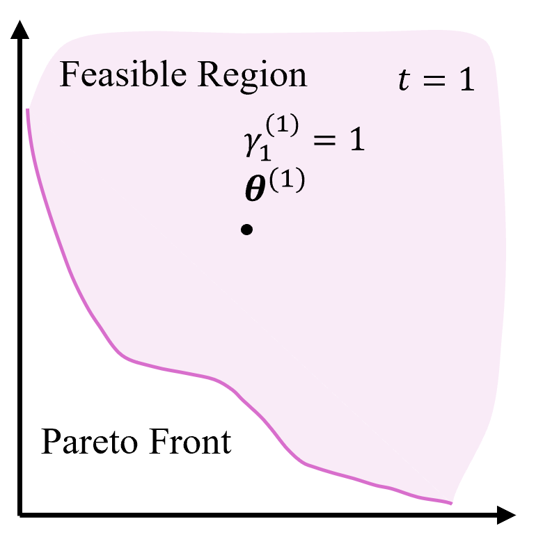
(a)

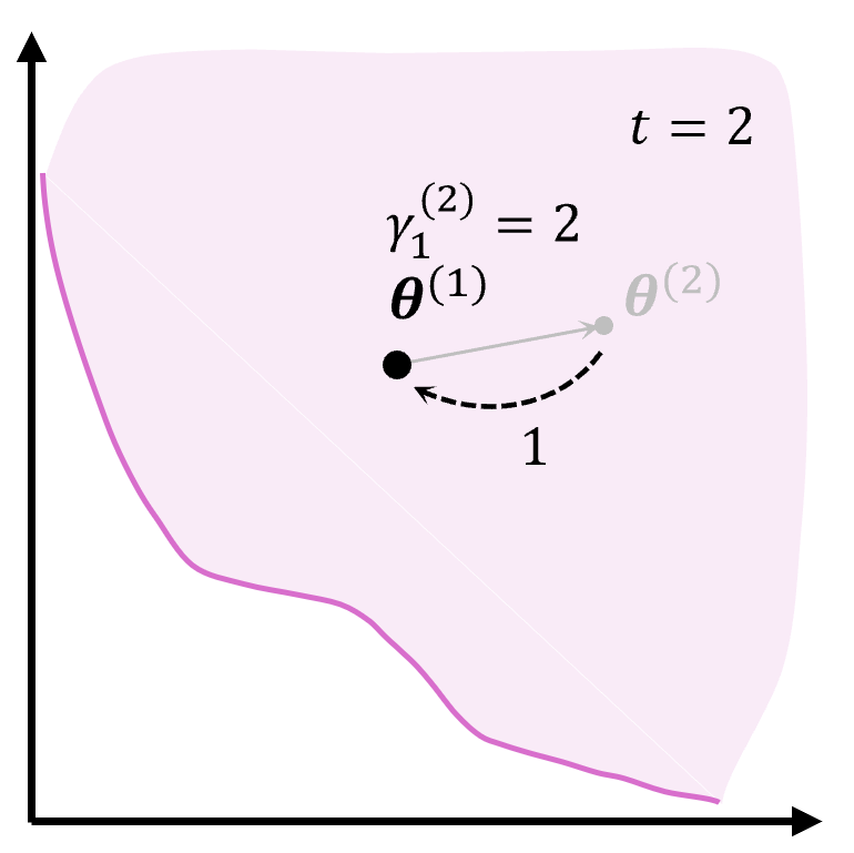
(b)

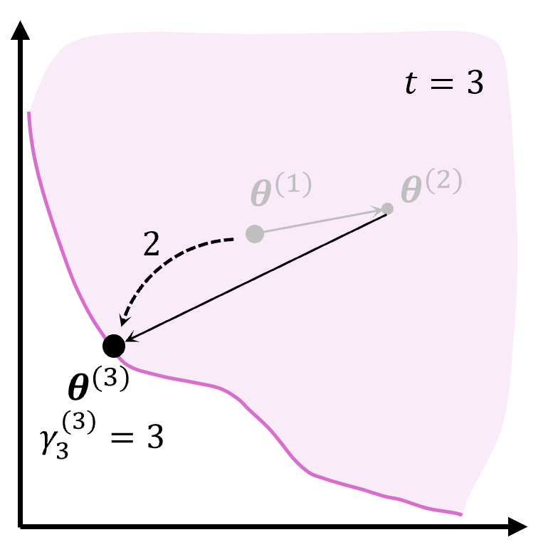
(c)

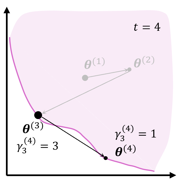
(d)

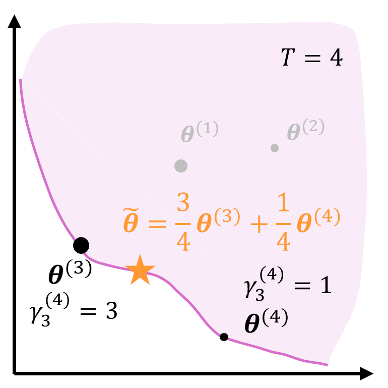
(e)

Figure 1: A Sample Run of AdaOMD-TCH. Solid arrows indicate search trajectories; dotted arrows indicate weight transfers. Black iterates are in the current Pareto optimal set; shaded ones are discarded. (a) $\bm{\theta}^{(1)}$ is added to $\mathcal{P}^{(1)}$ with a unit weight $\gamma^{(1)}_{1}=1$. (b) $\bm{\theta}^{(2)}\succeq\bm{\theta}^{(1)}$ is discarded with its weight transferred to $\bm{\theta}^{(1)}$. (c) $\bm{\theta}^{(3)}\preceq\bm{\theta}^{(1)}$ is added to $\mathcal{P}^{(3)}$ with its unit weight plus those of $\bm{\theta}^{(1)}$. $\bm{\theta}^{(1)}$ is discarded. (d) $\bm{\theta}^{(4)}$ is a new Pareto optimal iterate and added to $\mathcal{P}^{(4)}$ with $\gamma^{(4)}_{4}=1$. (e) The final output $\tilde{\bm{\theta}}$ is a weighted average of iterates in $\mathcal{P}^{(4)}$.

Like previous works applying OMD to the minimax fairness objective (He et al., 2024), Algorithm 1 adopts the traditional online-to-batch conversion that outputs the uniformly averaged solution $\bar{\bm{\theta}}$. Although it enjoys a convergence guarantee, as later stated in Section 3.3, it is unclear whether the conversion should involve every iterate, especially those dominated by new solutions as training proceeds. Motivated by this concern, we propose an adaptive conversion scheme that selectively excludes suboptimal iterates while retaining the same convergence guarantees. For readers to quickly grasp the key idea of this adaptive scheme, we first present the properties of its final solution before elaborating on the algorithmic implementation.

Key idea. Our final solution can be expresses as:

$$\tilde{\bm{\theta}}=\frac{1}{T}\sum_{\bm{\theta}^{(\tau)}\in\mathcal{P}}\gamma_{\tau}\bm{\theta}^{(\tau)},$$ (14)

with the following properties:

• $\mathcal{P}=\{\bm{\theta}^{(\tau)},\tau\in[T]\mid\nexists t\in[T]\ s.t.\ \bm{\theta}^{(t)}\preceq\bm{\theta}^{(\tau)}\}$ is the set of iterates not dominated by any other, i.e., Pareto optimal iterates.

• The construction of $\{\gamma_{\tau}\}$ can be summarized as:

  1. Assign each iterate $\bm{\theta}^{(t)}$ a unit weight of 1.

  2. For each $\bm{\theta}^{(t)}\notin\mathcal{P}$, distribute its unit weight, not necessarily uniformly, among $\{\bm{\theta}^{(\tau)}\in\mathcal{P}\mid\bm{\theta}^{(\tau)}\preceq\bm{\theta}^{(t)}\}$, i.e., Pareto optimal iterates that dominates $\bm{\theta}^{(t)}$.

  By this redistribution, we have $\sum_{\bm{\theta}^{(\tau)}\in\mathcal{P}}\gamma_{\tau}=T$, which ensures the correct scale of $\tilde{\bm{\theta}}$.

In short, $\tilde{\bm{\theta}}$ excludes a large number of insufficiently trained solutions by being a weighted average of Pareto optimal iterates only, with each one’s weight inherited from suboptimal iterates it dominates. This conversion is “adaptive” in the sense that $\mathcal{P}$ and $\{\gamma_{\tau}\}$ adapt to the actual searching trajectory, rather than being fixed in advance. We show that $\tilde{\bm{\theta}}$ achieves the same convergence rates as $\bar{\bm{\theta}}$ in the next subsection, and demonstrate its empirical superiority in Section 4.

Algorithmic implementation. We now introduce AdaOMD-TCH that outputs $\tilde{\bm{\theta}}$, as summarized in Algorithm 2. The key additional steps compared to Algorithm 1 are from lines 6 to 22, where we dynamically maintain a set $\mathcal{P}^{(t)}$ to be the Pareto optimal iterates up to round $t$, together with their weights $\bm{\gamma}^{(t)}$. Specifically, we handle each new candidate $\bm{\theta}^{(t)}$ by three cases:

• If $\bm{\theta}^{(t)}$ is dominated by some iterates in $\mathcal{P}^{(t-1)}$ ($A\neq\emptyset$ at line 7), directly discard $\bm{\theta}^{(t)}$ (line 9) and equally split its unit weight to those dominating set elements (lines 10 to 12).

• If $\bm{\theta}^{(t)}$ dominates some iterates in $\mathcal{P}^{(t-1)}$ ($B\neq\emptyset$ at line 17), delete the suboptimal elements (lines 19 and 20) and add $\bm{\theta}^{(t)}$ to the set (line 14) with its unit weight plus the sum of weights inherited from the deleted elements (lines 15 and 18).

• If $\bm{\theta}^{(t)}$ is not dominated by nor dominating any element in $\mathcal{P}^{(t-1)}$, i.e., it is a new temporary Pareto optimal iterate, add $\bm{\theta}^{(t)}$ to the set with a unit weight of 1 (lines 14 and 15).

Algorithm 2 AdaOMD-TCH

  Input: Number of rounds $T$, step sizes $\eta_{\bm{\theta}}$ and $\eta_{\bm{\lambda}}$.

  Initialize $\bm{\theta}^{(1)}$ and $\bm{\lambda}^{(1)}=(\frac{1}{m},\cdots,\frac{1}{m})^{\top}$.

  Initialize $\mathcal{P}^{(0)}=\bm{\gamma}^{(0)}=\emptyset$.

  for round $t=1,\cdots,T$ do

     Evaluate $f_{i}(\bm{\theta}^{(t)})$, $\nabla f_{i}(\bm{\theta}^{(t)})$, for all $i\in[m]$.

     Update $\mathcal{P}^{(t)}$ and $\bm{\gamma}^{(t)}$: // adaptive conversion

        $A\leftarrow\{\bm{\theta}^{(\tau)}\in\mathcal{P}^{(t-1)}\mid\bm{\theta}^{(\tau)}\preceq\bm{\theta}^{(t)}\}$.

        if $A\neq\emptyset$ then

           $\mathcal{P}^{(t)}\leftarrow\mathcal{P}^{(t-1)}$, $\bm{\gamma}^{(t)}\leftarrow\bm{\gamma}^{(t-1)}$.

           for $\bm{\theta}^{(\tau)}\in A$ do

              $\gamma^{(t)}_{\tau}\leftarrow\gamma^{(t)}_{\tau}+\frac{1}{|A|}$.

           end for

        else

           $\mathcal{P}^{(t)}\leftarrow\mathcal{P}^{(t-1)}\cup\{\bm{\theta}^{(t)}\}$.

           $\bm{\gamma}^{(t)}\leftarrow\bm{\gamma}^{(t-1)}\cup\{\gamma^{(t)}_{t}=1\}$.

           $B\leftarrow\{\bm{\theta}^{(\tau)}\in\mathcal{P}^{(t-1)}\mid\bm{\theta}^{(t)}\preceq\bm{\theta}^{(\tau)}\}$.

           if $B\neq\emptyset$ then

              $\gamma^{(t)}_{t}\leftarrow\gamma^{(t)}_{t}+\sum_{\bm{\theta}^{(\tau)}\in B}\gamma^{(t)}_{\tau}$.

              $\mathcal{P}^{(t)}\leftarrow\mathcal{P}^{(t)}\setminus B$.

              $\bm{\gamma}^{(t)}\leftarrow\bm{\gamma}^{(t)}\setminus\{\gamma^{(t)}_{\tau}\}_{\bm{\theta}^{(\tau)}\in B}$.

           end if

        end if

     Calculate $\bm{\lambda}^{(t+1)}$ and $\bm{\theta}^{(t+1)}$ as in OMD-TCH.

  end for

  Output: $\tilde{\bm{\theta}}=\frac{1}{T}\sum_{\bm{\theta}^{(\tau)}\in\mathcal{P}^{(T)}}\gamma_{\tau}^{(T)}\bm{\theta}^{(\tau)}$.

Figure 1 provides a detailed illustration. The aforementioned properties can be easily checked: when the algorithm finishes, $\mathcal{P}^{(T)}$ is exactly $\mathcal{P}$; the construction of $\{\gamma_{\tau}\}$ happens at each step, where we first assign a unit weight to the new iterate and then reallocate the weights of iterates that becomes suboptimal.

Complexity analysis. The memory complexity of AdaOMD-TCH is determined by the instantaneous size of $\mathcal{P}^{(t)}$. In practice, most elements in the current optimal set are immediately dominated and replaced by new iterates as training proceeds. Hence, we often have a sufficiently small size for $\mathcal{P}^{(t)}$. The time complexity mainly depends on the efficiency of querying, insertion, and deletion on $\mathcal{P}^{(t)}$. With advanced data structures such as k-d trees, such operations can be optimized to a logarithm complexity with respect to the set size on average. In our experiments, we directly adopt naive traversal for simplicity.

3.3 Theoretical Convergence Guarantees

In this section, we formally state the convergence guarantees for OMD-TCH and AdaOMD-TCH. In regard to the consistently observed superiority of batch and stochastic gradient descent over their deterministic counterpart, we directly consider the stochastic setting. In the followings, we use $\delta f_{i}(\bm{\theta})$ to denote the stochastic gradient computed on a randomly sampled batch and $\nabla f_{i}(\bm{\theta})$ to denote the true gradient. The $\nabla$’s in Algorithms 1 and 2 should be replaced with the corresponding $\delta$’s. We adopt the following assumptions commonly used in convergence analysis:

Assumption 1.

With $\|\mathbf{x}\|_{\infty}=\underset{i\in[d]}{\max}\ |x_{i}|$ for $\mathbf{x}\in\mathbb{R}^{d}$ being the infinity norm:

1. Convexity: $\forall i\in[m]$, $f_{i}(\bm{\theta})$ is convex in $\bm{\theta}$.

2. Bounded objectives: $\forall i\in[m],\forall\bm{\theta}\in\Theta,f_{i}(\bm{\theta})\leq U$.

3. Bounded gradients and stochastic gradients: $\forall i\in[m],\forall\bm{\theta}\in\Theta,\|\nabla f_{i}(\bm{\theta})\|_{\infty}\leq L,\|\delta f_{i}(\bm{\theta})\|_{\infty}\leq L$.

4. Bounded feasible region: $\forall\bm{\theta}\in\Theta,\|\bm{\theta}\|_{\infty}\leq R_{\bm{\theta}}$.

Now, we first present the general convergence rates using OMD instances induced by arbitrary distance generating functions $\psi_{\bm{\theta}}$ and $\psi_{\bm{\lambda}}$.

Theorem 3.

Suppose Assumption 1 holds. With $\psi_{\bm{\theta}}$, $\psi_{\bm{\lambda}}$, $\eta_{\bm{\theta}}$, and $\eta_{\bm{\lambda}}$ satisfying (1) $\psi_{\bm{\theta}}$ is $\mu_{\bm{\theta}}$-strongly convex, (2) $\psi_{\bm{\lambda}}$ is $\mu_{\bm{\lambda}}$-strongly convex, (3) $\eta_{\bm{\theta}}=\sqrt{\frac{4\mu_{\bm{\theta}}D_{\bm{\theta}}}{5TC_{\bm{\theta}}L^{2}}}$, and (4) $\eta_{\bm{\lambda}}=\sqrt{\frac{2\mu_{\bm{\lambda}}D_{\bm{\lambda}}}{3TC_{\bm{\lambda}}U^{2}}}$, both Algorithms 1 and 2 enjoy the following convergence guarantee:

$$\mathbb{E}\left[\operatorname{TCH}(\hat{\bm{\theta}};\mathbf{w})\right]-\underset{\bm{\theta}\in\Theta}{\min}\operatorname{TCH}(\bm{\theta};\mathbf{w})$$

$$\qquad\qquad\leq\sqrt{\frac{20D_{\bm{\theta}}C_{\bm{\theta}}L^{2}}{\mu_{\bm{\theta}}T}}+\sqrt{\frac{54D_{\bm{\lambda}}C_{\bm{\lambda}}U^{2}}{\mu_{\bm{\lambda}}T}}.$$ (15)

On the LHS, $\hat{\bm{\theta}}$ is either $\bar{\bm{\theta}}$ or $\tilde{\bm{\theta}}$, and the expectation is taken on the stochastic gradients. On the RHS, constants $D_{\bm{\theta}}$, $D_{\bm{\lambda}}$, $C_{\bm{\theta}}$, and $C_{\bm{\lambda}}$ depend on the choices of $\psi_{\bm{\theta}}$ and $\psi_{\bm{\lambda}}$, and are associated with the dimensions of $\bm{\theta}$ (i.e., $d$) and $\bm{\lambda}$ (i.e., $m$) respectively.

We provide the high-probability bound and proofs in Appendix A.1. Theorem 3 indicates that both OMD-TCH and AdaOMD-TCH converge at a rate of $O(1/\sqrt{T})$, matching batch or stochastic gradient descent in the dependency on the iteration round $T$.

To see the dependency on $d$ and $m$, we instantiate this general bound with specific choices of $\psi_{\bm{\theta}}$ and $\psi_{\bm{\lambda}}$: for $\bm{\theta}$, setting $\psi_{\bm{\theta}}(\bm{\theta})=\frac{1}{2}\|\bm{\theta}\|_{2}^{2}$, we have projected gradient descent; for $\bm{\lambda}$, we adopt either PGD or exponentiated gradient with $\psi_{\bm{\lambda}}=\frac{1}{2}\|\bm{\lambda}\|_{2}^{2}$ or $\psi_{\bm{\lambda}}=\sum_{i=1}^{m}\lambda_{i}\log\lambda_{i}$, i.e., the negative entropy. The specific bounds are:

Theorem 4.

Suppose Assumption 1 holds. Using PGD for both $\bm{\theta}$ and $\bm{\lambda}$, with optimal step sizes $\eta_{\bm{\theta}}=\sqrt{\frac{8R_{\bm{\theta}}^{2}}{5TL^{2}}}$ and $\eta_{\bm{\lambda}}=\sqrt{\frac{4}{3TmU^{2}}}$, both Algorithms 1 and 2 converge as follows, where $\hat{\bm{\theta}}$ is either $\bar{\bm{\theta}}$ or $\tilde{\bm{\theta}}$:

$$\mathbb{E}\left[\operatorname{TCH}(\hat{\bm{\theta}};\mathbf{w})\right]-\underset{\bm{\theta}\in\Theta}{\min}\operatorname{TCH}(\bm{\theta};\mathbf{w})$$

$$\qquad\qquad\leq\frac{2\sqrt{10}dR_{\bm{\theta}}L}{\sqrt{T}}+\frac{6\sqrt{3}\sqrt{m}U}{\sqrt{T}}.$$ (16)

Theorem 5.

Suppose Assumption 1 holds, using PGD for $\bm{\theta}$ and EG for $\bm{\lambda}$, with optimal step sizes $\eta_{\bm{\theta}}=\sqrt{\frac{8R_{\bm{\theta}}^{2}}{5TL^{2}}}$ and $\eta_{\bm{\lambda}}=\sqrt{\frac{2\log m}{3TU^{2}}}$, both Algorithms 1 and 2 converge converge as follows, where $\hat{\bm{\theta}}$ is either $\bar{\bm{\theta}}$ or $\tilde{\bm{\theta}}$:

$$\mathbb{E}\left[\operatorname{TCH}(\hat{\bm{\theta}};\mathbf{w})\right]-\underset{\bm{\theta}\in\Theta}{\min}\operatorname{TCH}(\bm{\theta};\mathbf{w})$$

$$\qquad\qquad\leq\frac{2\sqrt{10}dR_{\bm{\theta}}L}{\sqrt{T}}+\frac{3\sqrt{6}\sqrt{\log m}U}{\sqrt{T}}.$$ (17)

Proofs are provided in Appendix A.2. Comparing (16) and (17), one can see that using EG for $\bm{\lambda}$ gives a logarithm advantage in the convergence rate’s dependency on the number of objectives $m$, as in $O(\sqrt{\log m/T})$ over $O(\sqrt{m/T})$. Nevertheless, despite this theoretical superiority, we do not observe significant differences between the two instances in our experiments.

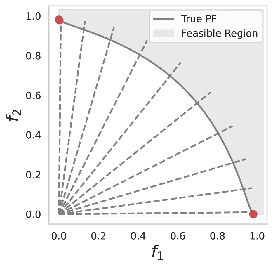
(a) LS

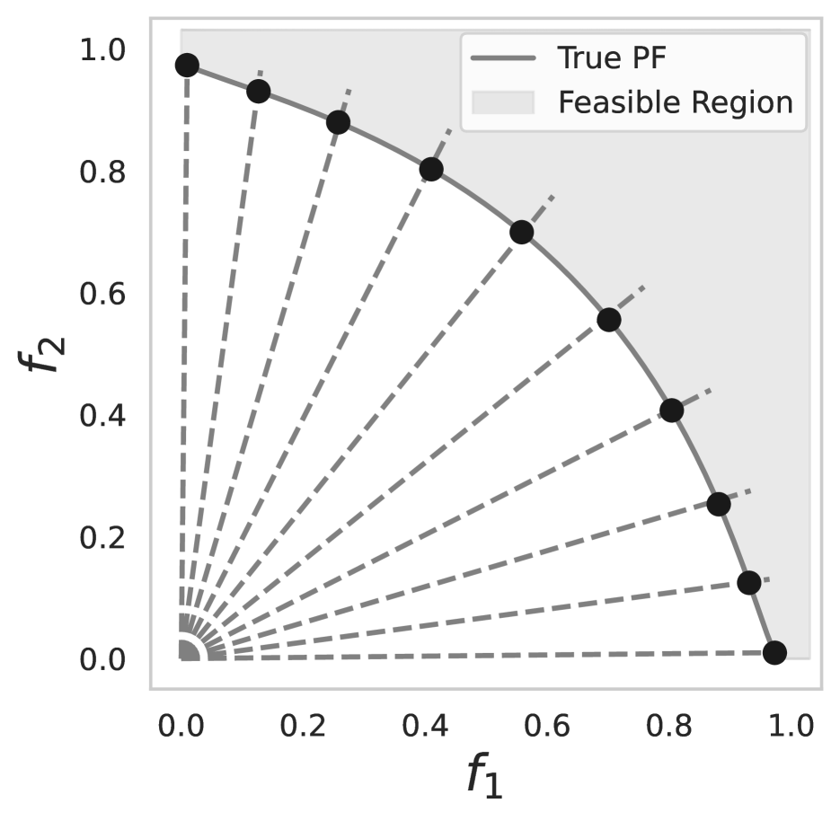
(b) TCH

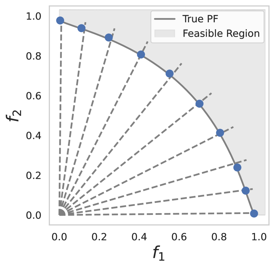
(c) OMDgd-TCH

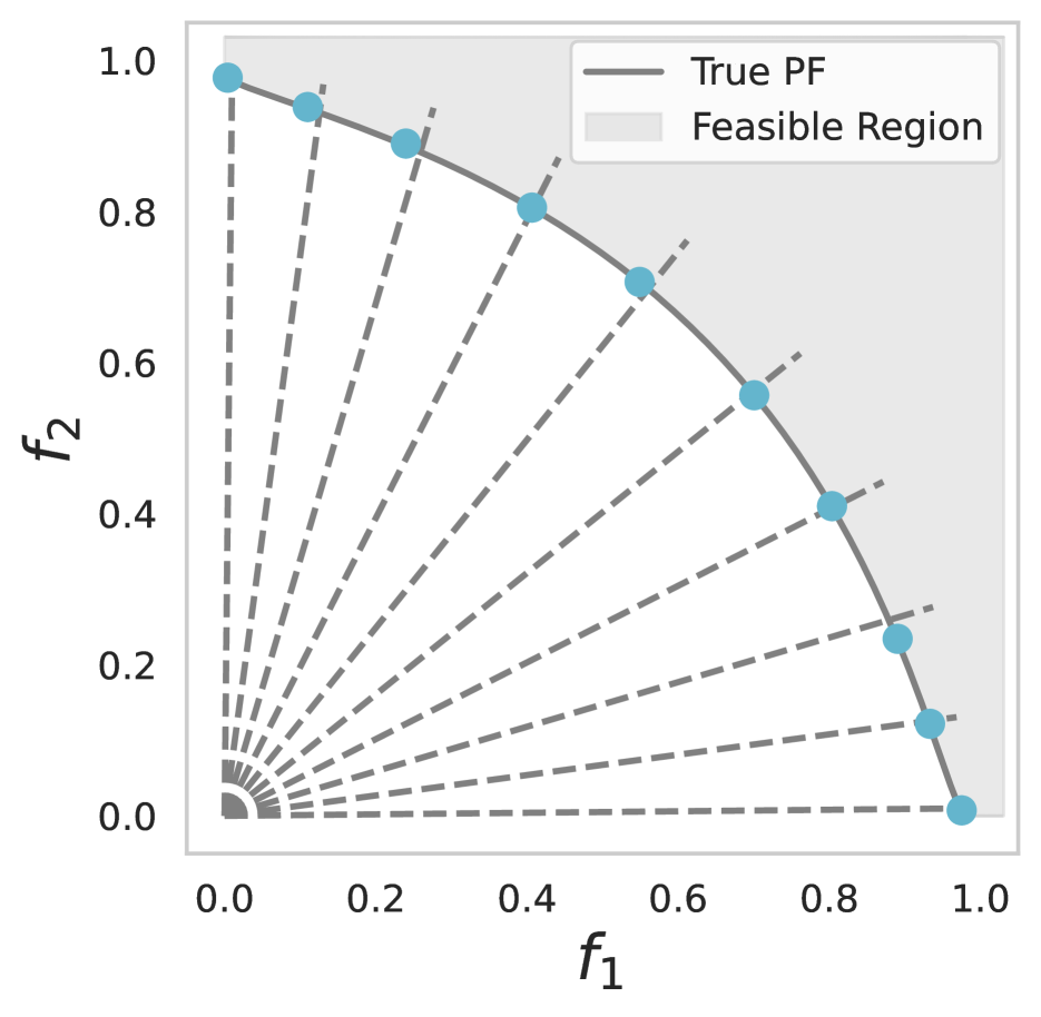
(d) AdaOMDgd-TCH

Figure 2: Solutions Found by Different Methods on the VLMOP2 Problem. Each dotted ray in a subfigure corresponds to the inverse of a preference vector. Results are averaged across 3 random seeds.

4 EXPERIMENTS

Our experimental studies mainly investigate two questions: (1) Can (Ada)OMD-TCH serve as a general MOO method for finding optimal solutions with diverse tradeoffs? (2) Is the proposed adaptive online-to-batch conversion scheme effective in improving practical performance over its uniform averaging counterpart? We provide affirmative evidence to these questions in Sections 4.1 (synthetic problem) and 4.2 (fair federated learning) respectively.

4.1 Finding Solutions with Diverse Trade-offs

In this section, we verify the ability of (Ada)OMD-TCH to find a diverse set of Pareto optimal solutions given different preference vector $\mathbf{w}$’s.

Problem setup. We adopt the widely studied VLMOP2 problem (Van Veldhuizen and Lamont, 1999) which has a non-convex PF with:

$$f_{1}(\bm{\theta}) =1-\exp\left(-\sum_{i=1}^{d}\left(\theta_{i}-\frac{1}{\sqrt{d}}\right)^{2}\right)$$ (18)

$$f_{2}(\bm{\theta}) =1-\exp\left(-\sum_{i=1}^{d}\left(\theta_{i}+\frac{1}{\sqrt{d}}\right)^{2}\right)$$ (19)

where $\bm{\theta}\in\mathbb{R}^{d}$ ($d=10$). Ten preferences $\mathbf{w}$ are evenly spaced between $[0,1]^{\top}$ and $[1,0]^{\top}$. Experiments are conducted using MOO library (Zhang et al., 2024b), with (Ada)OMD-TCH implemented in its framework. More details are listed in Appendix B.1.

Results. Figure 2 illustrates the solutions found by linear scalarization (LS), Tchebycheff scalarization (TCH), and (Ada)OMD-TCH with (projected) gradient descent applied to the dynamic $\bm{\lambda}$. Results are evaluated on averaged decision variable $\bm{\theta}$’s found with each preference vector over 3 random seeds. As expected, LS can only locate the two endpoints on the PF and completely misses the non-convex regions, while TCH yields equally scattered diverse solutions, which, by Theorem 1, are the intersection points of the PF and rays corresponding to the (element-wise)inverse of $\mathbf{w}$. Proposed as smooth solvers for TCH, we desire solutions produced by (Ada)OMD-TCH to resemble those found by vanilla TCH. As shown, both OMDgd-TCH and AdaOMDgd-TCH successfully recover the diverse solutions with minor errors. Full results for individual seeds and (Ada)OMDeg-TCH where $\bm{\lambda}$ is updated with exponentiated gradient are listed in Appendix B.1.

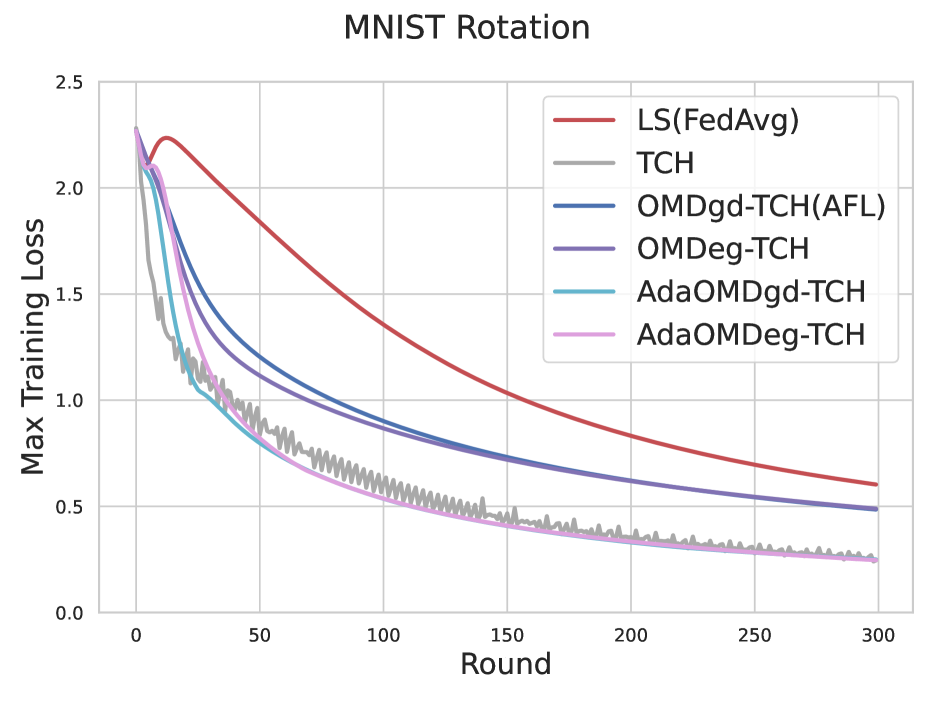
(a)

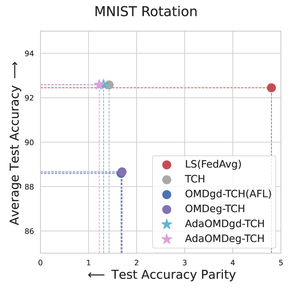
(b)

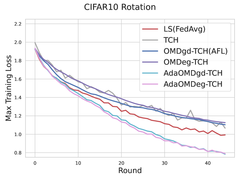
(c)

(d)

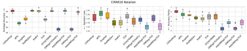
(e)

Figure 3: Federated Learning Results in Accuracy ($\uparrow$) and Fairness Metrics ($\downarrow$) on Rotated MNIST and CIFAR10. All results are averaged over 10 random seeds except for (a) and (c), which are plotted for seed=0 to show methods’ training fluctuations, with averaged results deferred to Appendix B.2.

4.2 Fair Federated Learning

One important application of MOO is to find the balanced trade-off optimal solution. Solving Tchebycheff scalarization with uniform preference is one natural approach by Theorem 1. Thus, we apply (Ada)OMD-TCH to such a problem — the accuracy-fairness challenge in Federated Learning (FL), where each client represents an objective, and achieving fairly equal performances across clients while maintaining overall accuracy is desired. As OMD has been adopted to solve this uniform preference case (Mohri et al., 2019), we particularly focus on how the adaptive conversion scheme improves over traditional conversion. As we will show, AdaOMD-TCH demonstrates comparable results to other state-of-the-art fair FL methods.

Baseline methods. We include FedAvg (McMahan et al., 2017b), and 6 state-of-the-art client-level fair FL methods: qFFL (Lin et al., 2019), AFL (Mohri et al., 2019), TERM (Li et al., 2020), FedFV (Wang et al., 2021), PropFair (Zhang et al., 2022), and FedMGDA+ (Hu et al., 2022b). Due to the same problem nature, many of them can be interpreted as a corresponding MOO method with uniform preference: FedAvg represents linear scalarization (LS), TERM has a highly similar loss function to smooth Tchebycheff (STCH), and FedMGDA+ is a mixture of LS and multiple gradient descent. In particular, AFL is equivalent to OMD-TCH with projected gradient descent, yet outputs the traditional time-averaged solution. The vanilla Tchebycheff scalarization (TCH) is also included. For a fair comparison, we focused on generic FL methods that train a shared global model rather than personalized approaches.

Data and models. We consider MNIST (Deng, 2012) and CIFAR10 (Krizhevsky and Hinton, 2009) datasets, and for each dataset, we simulate three scenarios of FL data heterogeneity for $m=10$ clients, following Ghosh et al. (2020); Collins et al. (2021):

• Rotation: All images of a client are rotated to the same degree $\psi$ where $\psi$ can be 90, 180, or 270.

• Partial class with C=2 or 5: Images of a client only come from 2 or 5 classes.

We train a two-layer fully connected neural network with ReLU activation functions for MNIST and a ResNet18 model (He et al., 2016) for CIFAR10. More implementation details on data settings and hyperparameter tuning are reported in Appendix B.2.

Evaluation metrics. The performance is measured two-fold: overall accuracy and client-level fairness. We use average test accuracy for the former, and two commonly used FL fairness metrics for the latter – agnostic loss (Mohri et al., 2019), i.e., the maximum client test loss, and accuracy parity (Li et al., 2019), i.e., the standard deviation of client test accuracies. Lower fairness metrics indicate a more fair FL model.

Results. Figure 3 offers a partial but representative summary. While OMD-TCH offers a relatively fairer solution in most cases, its overall accuracy is well below the baseline LS (FedAvg). AdaOMD-TCH exhibits significant improvements over OMD-TCH: during training, the worst client loss decreases steadily and more rapidly, and achieves a lower final value, as in Figures 3(a) and 3(c); at test time, Figures 3(b) and 3(d) show that average accuracy is increased to equal or even better level of LS (FedAvg), while deviations in accuracy parity remain minimal. Interestingly, although suffered from training oscillations, the vanilla TCH attains similar results to AdaOMD-TCH on MNIST, but degrades on CIFAR10. This may result from more complex data intensifying conflicts between objectives (clients), and optimizing only for the worst is no longer enough. Figure 3(e) includes more methods for comparison, where AdaOMD-TCH achieves competitive average accuracy, lower agnostic loss, and generally lower accuracy parity with values only slightly higher than OMD-TCH. Similar results are observed in other settings. More figures and tables are in Appendix B.2.

5 CONCLUSION

We propose OMD-TCH, a general solver for Tchebycheff scalarization in multi-objective optimization using online mirror descent that smooths out the hard one-hot update. We further propose AdaOMD-TCH by replacing the uniform online-to-batch conversion with a novel adaptive scheme that selectively discards suboptimal iterates while retaining the same convergence guarantees. Specifically, we prove an $O(\sqrt{\log m/T})$ convergence rate for both OMD-TCH and AdaOMD-TCH in the stochastic setting. Empirically, (Ada)OMD-TCH effectively recovers diverse solutions on a non-convex PF. When applied to fair federated learning problems, AdaOMD-TCH significantly improves over OMD-TCH, achieving state-of-the-art results in both accuracy and fairness metrics. We believe our methods serve as a powerful tool for multi-objective optimization and algorithmic fairness, and offer a new perspective in online-to-batch conversion.

Acknowledgements

Han Zhao is partially supported by an NSF IIS grant No. 2416897 and a Google Research Scholar Award.

APPENDICES

Appendix A provides the formal proof of Theorems 3, 4, and 5 in the main text. Appendix B includes complete experiment details and results.

A Proofs

A.1 Theorem 3: The Corresponding High-Probability Bound and Proofs

Theorem 6 (High-probability bound for Theorem 3).

Suppose Assumption 1 holds. With the same choices of $\psi_{\bm{\theta}}$, $\psi_{\bm{\lambda}}$, $\eta_{\bm{\theta}}$, and $\eta_{\bm{\lambda}}$ as in Theorem 3, both Algorithms 1 and 2 enjoy the convergence guarantee: with probability at least $1-\gamma$, $0<\gamma<1$,

$$\operatorname{TCH}(\hat{\bm{\theta}};\mathbf{w})-\underset{\bm{\theta}\in\Theta}{\min}\operatorname{TCH}(\bm{\theta};\mathbf{w})\leq\sqrt{\frac{20D_{\bm{\theta}}C_{\bm{\theta}}L^{2}}{\mu_{\bm{\theta}}T}}+\sqrt{\frac{54D_{\bm{\lambda}}C_{\bm{\lambda}}U^{2}}{\mu_{\bm{\lambda}}T}}++4dR_{\bm{\theta}}L\sqrt{\frac{2}{T}\log\frac{1}{\gamma}}+8U\sqrt{\frac{2}{T}\log\frac{1}{\gamma}},$$ (20)

where all notations are the same as Theorem 3.

We now prove both Theorems 3 and 6, which is based on several lemmas. We first establish the key lemma that fits the proof for $\tilde{\bm{\theta}}$, output by our adaptive online-to-batch conversion scheme, into the same analysis framework for $\bar{\bm{\theta}}$, output by the traditional uniform averaging conversion. Recall that $\mathcal{L}(\bm{\theta},\bm{\lambda};\mathbf{w})\coloneqq\sum_{i=1}^{m}\lambda_{i}\left(w_{i}f_{i}(\bm{\theta})\right)$.

Lemma 1.

Suppose Assumption 1 holds and $\tilde{\bm{\theta}}=\frac{1}{T}\sum_{\bm{\theta}^{(\tau)}\in\mathcal{P}}\gamma_{\tau}\bm{\theta}^{(\tau)}$ is the output of Algorithm 2 on iterates $\{\bm{\theta}^{(t)}\}_{t=1}^{T}$ and $\{\bm{\lambda}^{(t)}\}_{t=1}^{T}$. Then, for any $\bm{\lambda},\mathbf{w}\in\Delta_{m}$,

$$\mathcal{L}(\tilde{\bm{\theta}},\bm{\lambda};\mathbf{w})\leq\frac{1}{T}\sum_{t=1}^{T}\mathcal{L}(\bm{\theta}^{(t)},\bm{\lambda};\mathbf{w}).$$ (21)

Proof.

First, by Assumption 1, $f_{i}(\bm{\theta})$ is convex in $\bm{\theta}$, and hence so is $\mathcal{L}(\bm{\theta},\bm{\lambda};\mathbf{w})$. By convexity,

$$\mathcal{L}(\tilde{\bm{\theta}},\bm{\lambda};\mathbf{w})\leq\frac{1}{T}\sum_{\bm{\theta}^{(\tau)}\in\mathcal{P}}\gamma_{\tau}\mathcal{L}(\bm{\theta}^{(\tau)},\bm{\lambda};\mathbf{w}).$$ (22)

Now, to prove (21), it suffices to prove:

$$\frac{1}{T}\sum_{\bm{\theta}^{(\tau)}\in\mathcal{P}}\gamma_{\tau}\mathcal{L}(\bm{\theta}^{(\tau)},\bm{\lambda};\mathbf{w})\leq\frac{1}{T}\sum_{t=1}^{T}\mathcal{L}(\bm{\theta}^{(t)},\bm{\lambda};\mathbf{w})$$ (23)

In fact, this inequality naturally stems from how $\{\gamma_{\tau}\}$ are constructed through weight re-allocation, as stated in the properties of $\tilde{\bm{\theta}}$. To see this, we first specify some notations that describe the re-allocation:

• Suppose when Algorithm 2 finishes, for each $\bm{\theta}^{(t)}\notin\mathcal{P}$, its unit weight is re-allocated among elements in $P_{t}\subset\mathcal{P}$, with each $\bm{\theta}^{(\tau)}\in P_{t}$ recieving weight $\beta_{t\tau}$, such that $\sum_{\bm{\theta}^{(\tau)}\in P_{t}}\beta_{t\tau}=1$.

• On the other way round, for each $\bm{\theta}^{(\tau)}\in\mathcal{P}$, its weight $\gamma_{\tau}$, apart from its own unit weight, is inherited from $S_{\tau}\subset\mathcal{P}^{c}$, such that $1+\sum_{\bm{\theta}^{(t)}\in S_{\tau}}\beta_{t\tau}=\gamma_{\tau}$.

In each step, the weights of some suboptimal iterates are transferred to existing iterates that dominates them. By the transitivity of Pareto dominance, when the algorithm finishes, for any $\bm{\theta}^{(t)}\notin\mathcal{P}$ and $\bm{\theta}^{(\tau)}\in P_{t}$, we have $\bm{\theta}^{(\tau)}\preceq\bm{\theta}^{(t)}$. Therefore, $f_{i}(\bm{\theta}^{(\tau)})\leq f_{i}(\bm{\theta}^{(t)})$ for all $i\in[m]$, and consequently, for any $\bm{\lambda},\mathbf{w}\in\Delta_{m}$, we have:

$$\mathcal{L}(\bm{\theta}^{(\tau)},\bm{\lambda};\mathbf{w})\leq\mathcal{L}(\bm{\theta}^{(t)},\bm{\lambda};\mathbf{w}).$$ (24)

With this inequality, we have for each term on the RHS of (23) where $\bm{\theta}^{(t)}\notin\mathcal{P}$:

$$\mathcal{L}(\bm{\theta}^{(t)},\bm{\lambda};\mathbf{w}) =\sum_{\bm{\theta}^{(\tau)}\in P_{t}}\beta_{t\tau}\mathcal{L}(\bm{\theta}^{(t)},\bm{\lambda};\mathbf{w})\quad\quad\text{($\because\sum_{\bm{\theta}^{(\tau)}\in P_{t}}\beta_{t\tau}=1$)}$$

$$\geq\sum_{\bm{\theta}^{(\tau)}\in P_{t}}\beta_{t\tau}\mathcal{L}(\bm{\theta}^{(\tau)},\bm{\lambda};\mathbf{w}),$$ (25)

Finally, we can prove (23) by:

$$T\times\text{RHS} =\sum_{\bm{\theta}^{(\tau)}\in\mathcal{P}}\mathcal{L}(\bm{\theta}^{(\tau)},\bm{\lambda};\mathbf{w})+\sum_{\bm{\theta}^{(t)}\notin\mathcal{P}}\mathcal{L}(\bm{\theta}^{(t)},\bm{\lambda};\mathbf{w})$$

$$\geq\sum_{\bm{\theta}^{(\tau)}\in\mathcal{P}}\mathcal{L}(\bm{\theta}^{(\tau)},\bm{\lambda};\mathbf{w})+\sum_{\bm{\theta}^{(t)}\notin\mathcal{P}}\sum_{\bm{\theta}^{(\tau)}\in P_{t}}\beta_{t\tau}\mathcal{L}(\bm{\theta}^{(\tau)},\bm{\lambda};\mathbf{w})$$

$$=\sum_{\bm{\theta}^{(\tau)}\in\mathcal{P}}\mathcal{L}(\bm{\theta}^{(\tau)},\bm{\lambda};\mathbf{w})+\sum_{\bm{\theta}^{(\tau)}\in\mathcal{P}}\sum_{\bm{\theta}^{(t)}\in S_{\tau}}\beta_{t\tau}\mathcal{L}(\bm{\theta}^{(\tau)},\bm{\lambda};\mathbf{w})$$

$$=\sum_{\bm{\theta}^{(\tau)}\in\mathcal{P}}\left(1+\sum_{\bm{\theta}^{(t)}\in S_{\tau}}\beta_{t\tau}\right)\mathcal{L}(\bm{\theta}^{(\tau)},\bm{\lambda};\mathbf{w})$$

$$=\sum_{\bm{\theta}^{(\tau)}\in\mathcal{P}}\gamma_{\tau}\mathcal{L}(\bm{\theta}^{(\tau)},\bm{\lambda};\mathbf{w})=T\times\text{LHS},$$

which proves (21) and hence the lemma. ∎

Lemma 1 establishes a key inequality that allows us to continue the proof for $\tilde{\bm{\theta}}$ the same way as $\bar{\bm{\theta}}$, which follows the standard analysis of a minimax optimization problem. Before that, we refer to some established results.

Lemma 2 (Properties of Bregman divergence,  Chen and Teboulle (1993)).

Given a distance generating function $\psi:\mathcal{X}\rightarrow\mathbb{R}$ that is $\mu$-strongly convex w.r.t. a norm $\|\cdot\|:\mathcal{X}\rightarrow\mathbb{R}$ and continously differentiable on $\operatorname{int}\mathcal{X}$, the Bregman divergence $B_{\psi}:\mathcal{X}\times\operatorname{int}\mathcal{X}\rightarrow\mathbb{R}$ induced by $\psi$ is defined as:

$$B_{\psi}(\mathbf{x};\mathbf{y})=\psi(\mathbf{x})-\psi(\mathbf{y})-\langle\nabla\psi(\mathbf{y}),\mathbf{x}-\mathbf{y}\rangle.$$ (26)

Moreover, $B_{\psi}$ has the following properties:

• Non-negativity and convexity: $B_{\psi}\geq 0$ and is convex in the first argument.

• Lower bound: For any two points $\mathbf{x}\in\mathcal{X}$ and $\mathbf{y}\in\operatorname{int}\mathcal{X}$,

  $$B_{\psi}(\mathbf{x};\mathbf{y})\geq\frac{\mu}{2}\|\mathbf{x}-\mathbf{y}\|^{2}.$$ (27)

• Three-point identity: For any three points $\mathbf{x},\mathbf{y}\in\operatorname{int}\mathcal{X}$ and $\mathbf{z}\in\mathcal{X}$,

  $$B_{\psi}(\mathbf{z};\mathbf{y})-B_{\psi}(\mathbf{z};\mathbf{x})-B_{\psi}(\mathbf{x};\mathbf{y})=\langle\nabla\psi(\mathbf{y})-\nabla\psi(\mathbf{x}),\mathbf{x}-\mathbf{z}\rangle.$$ (28)

Lemma 3 (Cauchy–Schwarz inequality for dual norms,  Boyd and Vandenberghe (2004b)).

Suppose $\|\cdot\|_{*}$ is the dual norm of a norm $\|\cdot\|:\mathcal{X}\rightarrow\mathbb{R}$ defined as $\|\mathbf{x}\|_{*}\coloneqq\underset{\mathbf{y},\|\mathbf{y}\|\leq 1}{\max}\langle\mathbf{x},\mathbf{y}\rangle$. Then, for any $\mathbf{x},\mathbf{y}\in\mathcal{X}$, by definition,

$$\langle\mathbf{x},\mathbf{y}\rangle\leq\|\mathbf{x}\|_{*}\|\mathbf{y}\|.$$ (29)

Lemma 4 (Azuma–Hoeffding inequality on martingales,  Azuma (1967)).

A discrete-time stochastic process $\{X_{1},X_{2},X_{3},\ldots\}$ is a martingale with respect to a filtration $\{H_{1},H_{2},H_{3},\ldots\}$ if at any time $t$, $\mathbb{E}\left[|X_{t}|\right]<\infty$ and $\mathbb{E}\left[X_{t}\mid H_{1},\cdots,H_{t-1}\right]=X_{t-1}$. Suppose a martingale satisfies that $|X_{t}-X_{t-1}|\leq c_{t}$ almost surely, then, for all positive integers $T$ and all positive reals $\epsilon$,

$$P\left(X_{T}-X_{0}\geq\epsilon\right)\leq\exp(\frac{-\epsilon^{2}}{2\sum_{t=1}^{T}c_{t}^{2}}).$$ (30)

Based on Lemmas 2 and 3, we prove another useful lemma:

Lemma 5.

Given arbitrary sequence $\{\bm{\zeta}^{(1)},\cdots,\bm{\zeta}^{(T)}\}$, and sequence $\{\bm{\nu}^{(1)},\cdots,\bm{\nu}^{(T)}\}$ of the same dimension that is defined as:

$$\bm{\nu}^{(t+1)} =\underset{\bm{\nu}\in V}{\arg\min}\ \langle\bm{\zeta}^{(t)},\bm{\nu}-\bm{\nu}^{(t)}\rangle+\frac{1}{\eta_{\bm{\nu}}}B_{\psi_{\bm{\nu}}}(\bm{\nu};\bm{\nu}^{(t)}),$$ (31)

$$\text{or }\bm{\nu}^{(t+1)} =\underset{\bm{\nu}\in V}{\arg\max}\ \langle\bm{\zeta}^{(t)},\bm{\nu}-\bm{\nu}^{(t)}\rangle-\frac{1}{\eta_{\bm{\nu}}}B_{\psi_{\bm{\nu}}}(\bm{\nu};\bm{\nu}^{(t)}),$$ (32)

where $\eta_{\bm{\nu}}$ is a constant step size, $B_{\psi_{\bm{\nu}}}$ is the Bregman divergence induced by $\psi_{\bm{\nu}}:V\rightarrow\mathbb{R}$, and $\psi_{\bm{\nu}}$ is $\mu_{\bm{\nu}}$-strongly convex w.r.t. the norm $\|\cdot\|_{\bm{\nu}}$. Then, for any $\bm{u}\in V$,

$$\sum_{t=1}^{T}\langle\bm{\zeta}^{(t)},\bm{\nu}^{(t)}-\bm{u}\rangle \leq\frac{1}{\eta_{\bm{\nu}}}B_{\psi_{\bm{\nu}}}(\bm{u};\bm{\nu}^{(1)})+\frac{\eta_{\bm{\nu}}}{2\mu_{\bm{\nu}}}\sum_{t=1}^{T}\|\bm{\zeta}^{(t)}\|_{*}^{2}\ ,$$ (33)

$$\text{or respectively, }\sum_{t=1}^{T}\langle\bm{\zeta}^{(t)},\bm{u}-\bm{\nu}^{(t)}\rangle \leq\frac{1}{\eta_{\bm{\nu}}}B_{\psi_{\bm{\nu}}}(\bm{u};\bm{\nu}^{(1)})+\frac{\eta_{\bm{\nu}}}{2\mu_{\bm{\nu}}}\sum_{t=1}^{T}\|\bm{\zeta}^{(t)}\|_{*}^{2}\ ,$$ (34)

where $\|\cdot\|_{*}$ is the dual norm of $\|\cdot\|_{\bm{\nu}}$.

Proof.

Consider a single term on the LHS of (33),

$$\langle\bm{\zeta}^{(t)},\bm{\nu}^{(t)}-\bm{u}\rangle =\langle\bm{\zeta}^{(t)}+\frac{1}{\eta_{\bm{\nu}}}\nabla\psi_{\bm{\nu}}(\bm{\nu}^{(t+1)})-\frac{1}{\eta_{\bm{\nu}}}\nabla\psi_{\bm{\nu}}(\bm{\nu}^{(t)}),\bm{\nu}^{(t+1)}-\bm{u}\rangle\text{ (term A)}$$

$$\ \ \ \ \ +\langle\frac{1}{\eta_{\bm{\nu}}}\nabla\psi_{\bm{\nu}}(\bm{\nu}^{(t)})-\frac{1}{\eta_{\bm{\nu}}}\nabla\psi_{\bm{\nu}}(\bm{\nu}^{(t+1)}),\bm{\nu}^{(t+1)}-\bm{u}\rangle\text{ (term B)}$$

$$\ \ \ \ \ +\langle\bm{\zeta}^{(t)},\bm{\nu}^{(t)}-\bm{\nu}^{(t+1)}\rangle\text{ (term C)}.$$ (35)

We bound terms A and B + C respectively. First, observe rule (31), the entire function to be minimized on the RHS is convex w.r.t. $\bm{\nu}$. Then, by the optimality condition for $\bm{\nu}^{(t+1)}$ on this convex function, we have:

$$\ \ \ \ \ \langle\nabla_{\bm{\nu}}\left(\langle\bm{\zeta}^{(t)},\bm{\nu}-\bm{\nu}^{(t)}\rangle+\frac{1}{\eta_{\bm{\nu}}}B_{\psi_{\bm{\nu}}}(\bm{\nu};\bm{\nu}^{(t)})\right)\mid_{\bm{\nu}^{(t+1)}},\bm{u}-\bm{\nu}^{(t+1)}\rangle$$

$$=\langle\bm{\zeta}^{(t)}+\frac{1}{\eta_{\bm{\nu}}}\nabla\psi_{\bm{\nu}}(\bm{\nu}^{(t+1)})-\frac{1}{\eta_{\bm{\nu}}}\nabla\psi_{\bm{\nu}}(\bm{\nu}^{(t)}),\bm{u}-\bm{\nu}^{(t+1)}\rangle\geq 0,\ \ \ \forall\bm{u}\in V.$$

Hence, term A $\leq 0$. Next, we apply the three-point identity in Lemma 2 to term B:

B $$=\frac{1}{\eta_{\bm{\nu}}}\langle\nabla\psi_{\bm{\nu}}(\bm{\nu}^{(t)})-\nabla\psi_{\bm{\nu}}(\bm{\nu}^{(t+1)}),\bm{\nu}^{(t+1)}-\bm{u}\rangle$$

$$=\frac{1}{\eta_{\bm{\nu}}}\left(B_{\psi_{\bm{\nu}}}(\bm{u};\bm{\nu}^{(t)})-B_{\psi_{\bm{\nu}}}(\bm{u};\bm{\nu}^{(t+1)})-B_{\psi_{\bm{\nu}}}(\bm{\nu}^{(t+1)};\bm{\nu}^{(t)})\right).$$ (36)

Then, we have for term C:

C $$=\frac{1}{\eta_{\bm{\nu}}}\langle\eta_{\bm{\nu}}\bm{\zeta}^{(t)},\bm{\nu}^{(t)}-\bm{\nu}^{(t+1)}\rangle$$

$$\leq\frac{1}{\eta_{\bm{\nu}}}\|\eta_{\bm{\nu}}\bm{\zeta}^{(t)}\|_{*}\|\bm{\nu}^{(t)}-\bm{\nu}^{(t+1)}\|\text{ (by Lemma \ref{lm:ap-2})}$$

$$\leq\frac{1}{\eta_{\bm{\nu}}}\left(\frac{1}{2\mu_{\bm{\nu}}}\|\eta_{\bm{\nu}}\bm{\zeta}^{(t)}\|_{\bm{\nu},*}^{2}+\frac{\mu_{\bm{\nu}}}{2}\|\bm{\nu}^{(t)}-\bm{\nu}^{(t+1)}\|_{\bm{\nu}}^{2}\right).$$ (37)

Now, adding (36) and (37),

$$\text{B}+\text{C} =\frac{1}{\eta_{\bm{\nu}}}\left(B_{\psi_{\bm{\nu}}}(\bm{u};\bm{\nu}^{(t)})-B_{\psi_{\bm{\nu}}}(\bm{u};\bm{\nu}^{(t+1)})\underline{-B_{\psi_{\bm{\nu}}}(\bm{\nu}^{(t+1)},\bm{\nu}^{(t)})}+\frac{1}{2\mu_{\bm{\nu}}}\|\eta_{\bm{\nu}}\bm{\zeta}^{(t)}\|_{\bm{\nu},*}^{2}+\underline{\frac{\mu_{\bm{\nu}}}{2}\|\bm{\nu}^{(t)}-\bm{\nu}^{(t+1)}\|_{\bm{\nu}}^{2}}\right)$$

$$\leq\frac{1}{\eta_{\bm{\nu}}}\left(B_{\psi_{\bm{\nu}}}(\bm{u};\bm{\nu}^{(t)})-B_{\psi_{\bm{\nu}}}(\bm{u};\bm{\nu}^{(t+1)})+\frac{\eta_{\bm{\nu}}^{2}}{2\mu_{\bm{\nu}}}\|\bm{\zeta}^{(t)}\|_{\bm{\nu},*}^{2}\right)\text{ (by the lower bound entry in Lemma \ref{lm:ap-1})}$$

$$=\frac{1}{\eta_{\bm{\nu}}}\left(B_{\psi_{\bm{\nu}}}(\bm{u};\bm{\nu}^{(t)})-B_{\psi_{\bm{\nu}}}(\bm{u};\bm{\nu}^{(t+1)})\right)+\frac{\eta_{\bm{\nu}}}{2\mu_{\bm{\nu}}}\|\bm{\zeta}^{(t)}\|_{\bm{\nu},*}^{2}.$$ (38)

Therefore, given term A $\leq 0$ and (38), we have from (35):

$$\langle\bm{\zeta}^{(t)},\bm{\nu}^{(t)}-\bm{u}\rangle =A+(B+C)\leq\frac{1}{\eta_{\bm{\nu}}}\left(B_{\psi_{\bm{\nu}}}(\bm{u};\bm{\nu}^{(t)})-B_{\psi_{\bm{\nu}}}(\bm{u};\bm{\nu}^{(t+1)})\right)+\frac{\eta_{\bm{\nu}}}{2\mu_{\bm{\nu}}}\|\bm{\zeta}^{(t)}\|_{\bm{\nu},*}^{2}.$$

Finally, by summing up both sides from $t=1$ to $T$, we have

$$\sum_{t=1}^{T}\langle\bm{\zeta}^{(t)},\bm{\nu}^{(t)}-\bm{u}\rangle \leq\frac{1}{\eta_{\bm{\nu}}}\left(B_{\psi_{\bm{\nu}}}(\bm{u};\bm{\nu}^{(1)})\underline{-B_{\psi_{\bm{\nu}}}(\bm{u};\bm{\nu}^{(T+1)})}\right)+\frac{\eta_{\bm{\nu}}}{2\mu_{\bm{\nu}}}\sum_{t=1}^{T}\|\bm{\zeta}^{(t)}\|_{\bm{\nu},*}^{2}$$

$$\leq\frac{1}{\eta_{\bm{\nu}}}B_{\psi_{\bm{\nu}}}(\bm{u};\bm{\nu}^{(1)})+\frac{\eta_{\bm{\nu}}}{2\mu_{\bm{\nu}}}\sum_{t=1}^{T}\|\bm{\zeta}^{(t)}\|_{\bm{\nu},*}^{2}\text{ (by non-negativity of $B_{\psi_{\bm{\nu}}}$)},$$

which proves (33). The maximization case can be proved by the same procedure utilizing the concavity of the function to be maximized in rule (32). ∎

Now, we are ready to prove Theorems 3 and 6.

Proof of Theorems 3 and 6.

Before starting the derivation, we obtain some bounds on the norm of gradients that will be used later. Directly implied by the assumptions, we have:

$$\|\nabla_{\bm{\theta}}\mathcal{L}(\bm{\theta},\bm{\lambda};\mathbf{w})\|_{\infty}=\|\bm{\lambda}\circ\mathbf{w}\circ\nabla\mathbf{f}(\bm{\theta})\|_{\infty}\leq\|\nabla\mathbf{f}(\bm{\theta})\|_{\infty}\leq L,$$ (39)

$$\|\nabla_{\bm{\lambda}}\mathcal{L}(\bm{\theta},\bm{\lambda};\mathbf{w})\|_{\infty}=\|\mathbf{w}\circ\mathbf{f}(\bm{\theta})\|_{\infty}\leq\|\mathbf{f}(\bm{\theta})\|_{\infty}\leq U.$$ (40)

The same upper bounds also hold for stochastic gradients. Now we begin our derivation. First, we rewrite the LHS of (15) with $\mathcal{L}(\bm{\theta},\bm{\lambda};\mathbf{w})$:

$$\operatorname{TCH}(\hat{\bm{\theta}};\mathbf{w})-\underset{\bm{\theta}\in\Theta}{\min}\operatorname{TCH}(\bm{\theta};\mathbf{w}) =\underset{\bm{\lambda}\in\Delta_{m}}{\max}\ \mathcal{L}(\hat{\bm{\theta}},\bm{\lambda};\mathbf{w})-\underset{\bm{\theta}}{\min}\underset{\bm{\lambda}\in\Delta_{m}}{\max}\ \mathcal{L}(\bm{\theta},\bm{\lambda};\mathbf{w}).$$ (41)

Given that $\mathcal{L}(\bm{\theta},\bm{\lambda};\mathbf{w})$ is convex in $\bm{\theta}$ and linear in $\bm{\lambda}$, we have:

$$\underset{\bm{\lambda}\in\Delta_{m}}{\max}\ \mathcal{L}(\hat{\bm{\theta}},\bm{\lambda};\mathbf{w})-\underset{\bm{\theta}}{\min}\underset{\bm{\lambda}\in\Delta_{m}}{\max}\ \mathcal{L}(\bm{\theta},\bm{\lambda};\mathbf{w}) =\underset{\bm{\lambda}\in\Delta_{m}}{\max}\ \mathcal{L}(\hat{\bm{\theta}},\bm{\lambda};\mathbf{w})-\underset{\bm{\lambda}\in\Delta_{m}}{\max}\underset{\bm{\theta}}{\min}\ \mathcal{L}(\bm{\theta},\bm{\lambda};\mathbf{w})\text{ (Von Neumann's theorem)}$$

$$\leq\underset{\bm{\lambda}\in\Delta_{m}}{\max}\ \mathcal{L}(\hat{\bm{\theta}},\bm{\lambda};\mathbf{w})-\underset{\bm{\theta}}{\min}\ \mathcal{L}(\bm{\theta},\bar{\bm{\lambda}};\mathbf{w})$$

$$=\mathcal{L}(\hat{\bm{\theta}},\bm{\lambda}^{*};\mathbf{w})-\mathcal{L}(\bm{\theta}^{*},\bar{\bm{\lambda}};\mathbf{w}),$$ (42)

where $\bm{\lambda}^{*}\coloneqq\underset{\bm{\lambda}\in\Delta_{m}}{\arg\max}\ \mathcal{L}(\hat{\bm{\theta}},\bm{\lambda};\mathbf{w})$, $\bm{\theta}^{*}\coloneqq\underset{\bm{\theta}}{\arg\min}\ \mathcal{L}(\bm{\theta},\bar{\bm{\lambda}};\mathbf{w})$, and $\bar{\bm{\lambda}}=\frac{1}{T}\sum_{t=2}^{T+1}\bm{\lambda}^{(t)}$. Here, $\bar{\bm{\lambda}}$ is deliberately averaged from $t=2$ to $T+1$ to match the update rule of $\bm{\theta}^{(t+1)}$ that is based on $\bm{\lambda}^{(t+1)}$ instead of $\bm{\lambda}^{(t)}$. This will be pointed out again when we make use of the update rule.

Next, by $\mathcal{L}(\bm{\theta},\bm{\lambda};\mathbf{w})$’s convexity in $\bm{\theta}$, we have for $\hat{\bm{\theta}}$ being $\bar{\bm{\theta}}$ and $\tilde{\bm{\theta}}$ respectively:

$$\mathcal{L}(\bar{\bm{\theta}},\bm{\lambda}^{*};\mathbf{w})\leq\frac{1}{T}\sum_{t=1}^{T}\mathcal{L}(\bm{\theta}^{(t)},\bm{\lambda}^{*};\mathbf{w}),$$ (43)

$$\mathcal{L}(\tilde{\bm{\theta}},\bm{\lambda}^{*};\mathbf{w})\leq\frac{1}{T}\sum_{\bm{\theta}^{(\tau)}\in\mathcal{P}}\gamma_{\tau}\mathcal{L}(\bm{\theta}^{(t)},\bm{\lambda}^{*};\mathbf{w})\leq\frac{1}{T}\sum_{t=1}^{T}\mathcal{L}(\bm{\theta}^{(t)},\bm{\lambda}^{*};\mathbf{w}),$$ (44)

where the second inequality in (44) is exactly Lemma 1. With the same RHS in (43) and (44), we are able to continue the proof for both solutions output by the traditional uniform averaging conversion and the new adaptive conversion. Next, by $\mathcal{L}(\bm{\theta},\bm{\lambda};\mathbf{w})$’s linearity in $\bm{\lambda}$, we have:

$$\mathcal{L}(\bm{\theta}^{*},\bar{\bm{\lambda}};\mathbf{w})=\frac{1}{T}\sum_{t=2}^{T+1}\mathcal{L}(\bm{\theta}^{*},\bm{\lambda}^{(t)};\mathbf{w})=\frac{1}{T}\sum_{t=1}^{T}\mathcal{L}(\bm{\theta}^{*},\bm{\lambda}^{(t+1)};\mathbf{w}).$$ (45)

With (43), (44), and (45), we continue from (42),

$$\mathcal{L}(\hat{\bm{\theta}},\bm{\lambda}^{*};\mathbf{w})-\mathcal{L}(\bm{\theta}^{*},\bar{\bm{\lambda}};\mathbf{w}) \leq\frac{1}{T}\sum_{t=1}^{T}\mathcal{L}(\bm{\theta}^{(t)},\bm{\lambda}^{*};\mathbf{w})-\frac{1}{T}\sum_{t=1}^{T}\mathcal{L}(\bm{\theta}^{*},\bm{\lambda}^{(t+1)};\mathbf{w})$$

$$=\frac{1}{T}\sum_{t=1}^{T}\left(\underbrace{\mathcal{L}(\bm{\theta}^{(t)},\bm{\lambda}^{*};\mathbf{w})-\mathcal{L}(\bm{\theta}^{(t)},\bm{\lambda}^{(t)};\mathbf{w})}_{\text{term A}}+\underbrace{\mathcal{L}(\bm{\theta}^{(t)},\bm{\lambda}^{(t+1)};\mathbf{w})-\mathcal{L}(\bm{\theta}^{*},\bm{\lambda}^{(t+1)};\mathbf{w})}_{\text{term B}}\right.$$

$$\ \ \ \ \ \ \ \ \ \ \ \ \ \ \left.+\underbrace{\mathcal{L}(\bm{\theta}^{(t)},\bm{\lambda}^{(t)};\mathbf{w})-\mathcal{L}(\bm{\theta}^{(t)},\bm{\lambda}^{(t+1)};\mathbf{w})}_{\text{term C}}\right).$$ (46)

Now, we bound A, B, and C by linearity, convexity, and linearity respectively:

$$\text{A}=\mathcal{L}(\bm{\theta}^{(t)},\bm{\lambda}^{*};\mathbf{w})-\mathcal{L}(\bm{\theta}^{(t)},\bm{\lambda}^{(t)};\mathbf{w})=\langle\nabla_{\bm{\lambda}}\mathcal{L}(\bm{\theta}^{(t)},\bm{\lambda}^{(t)};\mathbf{w}),\bm{\lambda}^{*}-\bm{\lambda}^{(t)}\rangle,$$

$$\text{B}=\mathcal{L}(\bm{\theta}^{(t)},\bm{\lambda}^{(t+1)};\mathbf{w})-\mathcal{L}(\bm{\theta}^{*},\bm{\lambda}^{(t+1)};\mathbf{w})\leq\langle\nabla_{\bm{\theta}}\mathcal{L}(\bm{\theta}^{(t)},\bm{\lambda}^{(t+1)};\mathbf{w}),\bm{\theta}^{(t)}-\bm{\theta}^{*}\rangle,$$

$$\text{C}=\mathcal{L}(\bm{\theta}^{(t)},\bm{\lambda}^{(t)};\mathbf{w})-\mathcal{L}(\bm{\theta}^{(t)},\bm{\lambda}^{(t+1)};\mathbf{w})=\langle\nabla_{\bm{\lambda}}\mathcal{L}(\bm{\theta}^{(t)},\bm{\lambda}^{(t)};\mathbf{w}),\bm{\lambda}^{(t)}-\bm{\lambda}^{(t+1)}\rangle.$$

We can then continue from (46):

$$\frac{1}{T}\sum_{t=1}^{T}(\text{A}+\text{B}+\text{C}) \leq\frac{1}{T}\sum_{t=1}^{T}\left(\langle\nabla_{\bm{\lambda}}\mathcal{L}(\bm{\theta}^{(t)},\bm{\lambda}^{(t)};\mathbf{w}),\bm{\lambda}^{*}-\bm{\lambda}^{(t)}\rangle+\langle\nabla_{\bm{\theta}}\mathcal{L}(\bm{\theta}^{(t)},\bm{\lambda}^{(t+1)};\mathbf{w}),\bm{\theta}^{(t)}-\bm{\theta}^{*}\rangle\right.$$

$$\ \ \ \ \ \ \ \ \ \ \ \ \ \left.+\langle\nabla_{\bm{\lambda}}\mathcal{L}(\bm{\theta}^{(t)},\bm{\lambda}^{(t)};\mathbf{w}),\bm{\lambda}^{(t)}-\bm{\lambda}^{(t+1)}\rangle\right)$$

$$=\frac{1}{T}\left(\sum_{t=1}^{T}\langle\delta_{\bm{\lambda}}\mathcal{L}(\bm{\theta}^{(t)},\bm{\lambda}^{(t)};\mathbf{w}),\bm{\lambda}^{*}-\bm{\lambda}^{(t)}\rangle\text{ (term D1)}\right.$$

$$\ \ \ \ \ \ \ \ +\sum_{t=1}^{T}\langle\nabla_{\bm{\lambda}}\mathcal{L}(\bm{\theta}^{(t)},\bm{\lambda}^{(t)};\mathbf{w})-\delta_{\bm{\lambda}}\mathcal{L}(\bm{\theta}^{(t)},\bm{\lambda}^{(t)};\mathbf{w}),\bm{\lambda}^{*}-\bm{\lambda}^{(t)}\rangle\text{ (term E1)}$$

$$\ \ \ \ \ \ \ \ +\sum_{t=1}^{T}\langle\delta_{\bm{\theta}}\mathcal{L}(\bm{\theta}^{(t)},\bm{\lambda}^{(t+1)};\mathbf{w}),\bm{\theta}^{(t)}-\bm{\theta}^{*}\rangle\text{ (term D2)}$$

$$\ \ \ \ \ \ \ \ +\sum_{t=1}^{T}\langle\nabla_{\bm{\theta}}\mathcal{L}(\bm{\theta}^{(t)},\bm{\lambda}^{(t+1)};\mathbf{w})-\delta_{\bm{\theta}}\mathcal{L}(\bm{\theta}^{(t)},\bm{\lambda}^{(t+1)};\mathbf{w}),\bm{\theta}^{(t)}-\bm{\theta}^{*}\rangle\text{ (term E2)}$$

$$\ \ \ \ \ \ \ \ +\sum_{t=1}^{T}\langle\delta_{\bm{\lambda}}\mathcal{L}(\bm{\theta}^{(t)},\bm{\lambda}^{(t)};\mathbf{w}),\bm{\lambda}^{(t)}-\bm{\lambda}^{(t+1)}\rangle\text{ (term D3)}$$

$$\ \ \ \ \ \ \ \ +\sum_{t=1}^{T}\left.\langle\nabla_{\bm{\lambda}}\mathcal{L}(\bm{\theta}^{(t)},\bm{\lambda}^{(t)};\mathbf{w})-\delta_{\bm{\lambda}}\mathcal{L}(\bm{\theta}^{(t)},\bm{\lambda}^{(t)};\mathbf{w}),\bm{\lambda}^{(t)}-\bm{\lambda}^{(t+1)}\rangle\right)\text{ (term E3)}.$$ (47)

This is the last reduction on the upper bound. After bounding the above five terms separately, we will be able to arrive at the inequalities in the theorem. Term D3 is upper bounded by 0, stemming from the update rule of $\bm{\lambda}$. All the rest can be solved by invoking Lemma 5. For D1 and D2, it is a direct application. For E1, E2, and E3, we need an additional construction step.

Bounding D3. We first get rid of D3 by the update rule of $\bm{\lambda}^{(t+1)}$:

$$\bm{\lambda}^{(t+1)}=\underset{\bm{\lambda}\in\Delta_{m}}{\arg\max}\ \langle\delta_{\bm{\lambda}}\mathcal{L}(\bm{\theta}^{(t)},\bm{\lambda}^{(t)};\mathbf{w}),\bm{\lambda}\rangle-\frac{1}{\eta_{\bm{\lambda}}}B_{\psi_{\bm{\lambda}}}(\bm{\lambda};\bm{\lambda}^{(t)})$$

$$\Rightarrow\langle\delta_{\bm{\lambda}}\mathcal{L}(\bm{\theta}^{(t)},\bm{\lambda}^{(t)};\mathbf{w}),\bm{\lambda}^{(t+1)}\rangle-\frac{1}{\eta_{\bm{\lambda}}}B_{\psi_{\bm{\lambda}}}(\bm{\lambda}^{(t+1)};\bm{\lambda}^{(t)})\geq\langle\delta_{\bm{\lambda}}\mathcal{L}(\bm{\theta}^{(t)},\bm{\lambda}^{(t)};\mathbf{w}),\bm{\lambda}^{(t)}\rangle-\frac{1}{\eta_{\bm{\lambda}}}B_{\psi_{\bm{\lambda}}}(\bm{\lambda}^{(t)};\bm{\lambda}^{(t)})$$

$$\Rightarrow\langle\delta_{\bm{\lambda}}\mathcal{L}(\bm{\theta}^{(t)},\bm{\lambda}^{(t)};\mathbf{w}),\bm{\lambda}^{(t+1)}\rangle\geq\langle\delta_{\bm{\lambda}}\mathcal{L}(\bm{\theta}^{(t)},\bm{\lambda}^{(t)};\mathbf{w}),\bm{\lambda}^{(t)}\rangle-0+\frac{1}{\eta_{\bm{\lambda}}}B_{\psi_{\bm{\lambda}}}(\bm{\lambda}^{(t+1)};\bm{\lambda}^{(t)})\geq\langle\delta_{\bm{\lambda}}\mathcal{L}(\bm{\theta}^{(t)},\bm{\lambda}^{(t)};\mathbf{w}),\bm{\lambda}^{(t)}\rangle$$

$$\text{D3}=\langle\delta_{\bm{\lambda}}\mathcal{L}(\bm{\theta}^{(t)},\bm{\lambda}^{(t)};\mathbf{w}),\bm{\lambda}^{(t)}-\bm{\lambda}^{(t+1)}\rangle\leq 0$$ (48)

Therefore, term D3 $\leq 0$ and can be eliminated when considering the upper bound.

Bounding D1. Now, for D1, recall the update rule for $\bm{\lambda}$:

$$\bm{\lambda}^{(t+1)}=\underset{\bm{\lambda}\in\Delta_{m}}{\arg\max}\ \langle\delta_{\bm{\lambda}}\mathcal{L}(\bm{\theta}^{(t)},\bm{\lambda}^{(t)};\mathbf{w}),\bm{\lambda}\rangle-\frac{1}{\eta_{\bm{\lambda}}}B_{\psi_{\bm{\lambda}}}(\bm{\lambda};\bm{\lambda}^{(t)}).$$

By Lemma 5, substituting $\bm{\zeta}^{(t)}=\delta_{\bm{\lambda}}\mathcal{L}(\bm{\theta}^{(t)},\bm{\lambda}^{(t)};\mathbf{w})$, $\bm{\nu}^{(t)}=\bm{\lambda}^{(t)}$, and $\bm{u}=\bm{\lambda}^{*}$, we have:

$$\text{D1}=\sum_{t=1}^{T}\langle\delta_{\bm{\lambda}}\mathcal{L}(\bm{\theta}^{(t)},\bm{\lambda}^{(t)};\mathbf{w}),\bm{\lambda}^{*}-\bm{\lambda}^{(t)}\rangle \leq\frac{1}{\eta_{\bm{\lambda}}}B_{\psi_{\bm{\lambda}}}(\bm{\lambda}^{*};\bm{\lambda}^{(1)})+\frac{\eta_{\bm{\lambda}}}{2\mu_{\bm{\lambda}}}\sum_{t=1}^{T}\|\delta_{\bm{\lambda}}\mathcal{L}(\bm{\theta}^{(t)},\bm{\lambda}^{(t)};\mathbf{w})\|_{\bm{\lambda},*}^{2}$$

$$\leq\frac{1}{\eta_{\bm{\lambda}}}D_{\bm{\lambda}}+\frac{\eta_{\bm{\lambda}}}{2\mu_{\bm{\lambda}}}TC_{\bm{\lambda}}U^{2},$$ (49)

where $\mu_{\bm{\lambda}}$ and $\|\cdot\|_{\bm{\lambda}}$ and is the constant and norm on which the strong convexity of $\psi_{\bm{\lambda}}$ is defined, and $\|\cdot\|_{\bm{\lambda},*}$ is the dual norm of $\|\cdot\|_{\bm{\lambda}}$. The upperbound of the norm stems from (40) at the beginning of the proof, and $C_{\bm{\lambda}}$, as well as $D_{\bm{\lambda}}$, are constants depending on the specific choice of $\psi_{\bm{\lambda}}$.

Bounding D2. Similarly, for D2, recall the update rule for $\bm{\theta}$:

$$\bm{\theta}^{(t+1)}=\underset{\bm{\theta}\in\Theta}{\arg\min}\ \langle\delta_{\bm{\theta}}\mathcal{L}(\bm{\theta}^{(t)},\bm{\lambda}^{(t+1)};\mathbf{w}),\bm{\theta}\rangle+\frac{1}{\eta_{\bm{\theta}}}B_{\psi_{\bm{\theta}}}(\bm{\theta};\bm{\theta}^{(t)}).$$

Note that the stochastic gradient is computed on $\bm{\lambda}^{(t+1)}$ instead of $\bm{\lambda}^{(t)}$. This is why we set $\bar{\bm{\lambda}}$ to be an average across $t=2$ to $T+1$. By Lemma 5, substituting $\bm{\zeta}^{(t)}=\delta_{\bm{\theta}}\mathcal{L}(\bm{\theta}^{(t)},\bm{\lambda}^{(t+1)};\mathbf{w})$, $\bm{\nu}^{(t)}=\bm{\theta}^{(t)}$, and $\bm{u}=\bm{\theta}^{*}$, we have:

$$\text{D2}=\sum_{t=1}^{T}\langle\delta_{\bm{\theta}}\mathcal{L}(\bm{\theta}^{(t)},\bm{\lambda}^{(t+1)};\mathbf{w}),\bm{\theta}^{(t)}-\bm{\theta}^{*}\rangle \leq\frac{1}{\eta_{\bm{\theta}}}B_{\psi_{\bm{\theta}}}(\bm{\theta}^{*};\bm{\theta}^{(1)})+\frac{\eta_{\bm{\theta}}}{2\mu_{\bm{\theta}}}\sum_{t=1}^{T}\|\delta_{\bm{\theta}}\mathcal{L}(\bm{\theta}^{(t)},\bm{\lambda}^{(t+1)};\mathbf{w})\|_{\bm{\theta},*}^{2}$$

$$\leq\frac{1}{\eta_{\bm{\theta}}}D_{\bm{\theta}}+\frac{\eta_{\bm{\theta}}}{2\mu_{\bm{\theta}}}TC_{\bm{\theta}}L^{2}.$$ (50)

Bounding E1. Next, for E1, the first argument of the inner product no longer matches the update rule for $\bm{\lambda}^{(t)}$ and thus Lemma 5 cannot be directly applied. Instead, we construct a sequence $\{\bm{\chi}^{(t)}\}$ such that

$$\bm{\chi}^{(1)}=\bm{\lambda}^{(1)},$$ (51)

$$\bm{\chi}^{(t+1)}=\underset{\bm{\chi}\in\Delta_{m}}{\arg\max}\ \langle\nabla_{\bm{\lambda}}\mathcal{L}(\bm{\theta}^{(t)},\bm{\lambda}^{(t)};\mathbf{w})-\delta_{\bm{\lambda}}\mathcal{L}(\bm{\theta}^{(t)},\bm{\lambda}^{(t)};\mathbf{w}),\bm{\chi}\rangle-\frac{1}{\eta_{\bm{\lambda}}}B_{\psi_{\bm{\lambda}}}(\bm{\chi};\bm{\chi}^{(t)}).$$ (52)

We invoke Lemma 5 on this sequence: substituting $\bm{\zeta}^{(t)}=\nabla_{\bm{\lambda}}\mathcal{L}(\bm{\theta}^{(t)},\bm{\lambda}^{(t)};\mathbf{w})-\delta_{\bm{\lambda}}\mathcal{L}(\bm{\theta}^{(t)},\bm{\lambda}^{(t)};\mathbf{w})$, $\bm{\nu}^{(t)}=\bm{\chi}^{(t)}$, and $\bm{u}=\bm{\lambda}^{*}$, we have:

$$\sum_{t=1}^{T}\langle\nabla_{\bm{\lambda}}\mathcal{L}(\bm{\theta}^{(t)},\bm{\lambda}^{(t)};\mathbf{w})-\delta_{\bm{\lambda}}\mathcal{L}(\bm{\theta}^{(t)},\bm{\lambda}^{(t)};\mathbf{w}),\bm{\lambda}^{*}-\bm{\chi}^{(t)}\rangle$$

$$\leq\frac{1}{\eta_{\bm{\lambda}}}B_{\psi_{\bm{\lambda}}}(\bm{\lambda}^{*};\bm{\lambda}^{(1)})+\frac{\eta_{\bm{\lambda}}}{2\mu_{\bm{\lambda}}}\sum_{t=1}^{T}\|\nabla_{\bm{\lambda}}\mathcal{L}(\bm{\theta}^{(t)},\bm{\lambda}^{(t)};\mathbf{w})-\delta_{\bm{\lambda}}\mathcal{L}(\bm{\theta}^{(t)},\bm{\lambda}^{(t)};\mathbf{w})\|_{\bm{\lambda},*}^{2}$$

$$\leq\frac{1}{\eta_{\bm{\lambda}}}B_{\psi_{\bm{\lambda}}}(\bm{\lambda}^{*};\bm{\lambda}^{(1)})+\frac{\eta_{\bm{\lambda}}}{2\mu_{\bm{\lambda}}}\sum_{t=1}^{T}\left(\|\nabla_{\bm{\lambda}}\mathcal{L}(\bm{\theta}^{(t)},\bm{\lambda}^{(t)};\mathbf{w})\|_{\bm{\lambda},*}+\|\delta_{\bm{\lambda}}\mathcal{L}(\bm{\theta}^{(t)},\bm{\lambda}^{(t)};\mathbf{w})\|_{\bm{\lambda},*}\right)^{2}$$

$$\leq\frac{1}{\eta_{\bm{\lambda}}}D_{\bm{\lambda}}+\frac{\eta_{\bm{\lambda}}}{2\mu_{\bm{\lambda}}}T4C_{\bm{\lambda}}U^{2}.$$ (53)

Then, we have for E1:

E1 $$=\sum_{t=1}^{T}\langle\nabla_{\bm{\lambda}}\mathcal{L}(\bm{\theta}^{(t)},\bm{\lambda}^{(t)};\mathbf{w})-\delta_{\bm{\lambda}}\mathcal{L}(\bm{\theta}^{(t)},\bm{\lambda}^{(t)};\mathbf{w}),\bm{\lambda}^{*}-\bm{\chi}^{(t)}\rangle$$

$$\ \ \ \ +\sum_{t=1}^{T}\langle\nabla_{\bm{\lambda}}\mathcal{L}(\bm{\theta}^{(t)},\bm{\lambda}^{(t)};\mathbf{w})-\delta_{\bm{\lambda}}\mathcal{L}(\bm{\theta}^{(t)},\bm{\lambda}^{(t)};\mathbf{w}),\bm{\chi}^{(t)}-\bm{\lambda}^{(t)}\rangle,$$ (54)

where the first term is bounded by (53). Different ways to deal with the second term result in the expectation bound and the high-probability bound respectively. First, we have by the total law of expectation:

$$\mathbb{E}\left[\sum_{t=1}^{T}\langle\nabla_{\bm{\lambda}}\mathcal{L}(\bm{\theta}^{(t)},\bm{\lambda}^{(t)};\mathbf{w})-\delta_{\bm{\lambda}}\mathcal{L}(\bm{\theta}^{(t)},\bm{\lambda}^{(t)};\mathbf{w}),\bm{\chi}^{(t)}-\bm{\lambda}^{(t)}\rangle\right]$$

$$=\sum_{t=1}^{T}\mathbb{E}\left[\mathbb{E}\left[\langle\nabla_{\bm{\lambda}}\mathcal{L}(\bm{\theta}^{(t)},\bm{\lambda}^{(t)};\mathbf{w})-\delta_{\bm{\lambda}}\mathcal{L}(\bm{\theta}^{(t)},\bm{\lambda}^{(t)};\mathbf{w}),\bm{\chi}^{(t)}-\bm{\lambda}^{(t)}\rangle\mid\eta_{1},\ldots,\eta_{t-1}\right]\right]$$

$$=\sum_{t=1}^{T}\mathbb{E}\left[\langle\bm{\chi}^{(t)}-\bm{\lambda}^{(t)},\mathbb{E}\left[\nabla_{\bm{\lambda}}\mathcal{L}(\bm{\theta}^{(t)},\bm{\lambda}^{(t)};\mathbf{w})-\delta_{\bm{\lambda}}\mathcal{L}(\bm{\theta}^{(t)},\bm{\lambda}^{(t)};\mathbf{w})\mid\eta_{1},\ldots,\eta_{t-1}\right]\rangle\right]$$ (55)

$$=\sum_{t=1}^{T}\mathbb{E}\left[\langle\bm{\chi}^{(t)}-\bm{\lambda}^{(t)},\bm{0}\rangle\right]=0,$$ (56)

where $\{\eta_{t}\}$ are the random batch sampled in the past to compute stochastic gradient. Here, (55) is based on the fact that both $\bm{\chi}^{(t)}$ and $\bm{\lambda}^{(t)}$ are deterministic given $\delta_{\bm{\lambda}}\mathcal{L}(\bm{\theta}^{(t-1)},\bm{\lambda}^{(t-1)};\mathbf{w})$, $\bm{\theta}^{(t-1)}$, and $\bm{\lambda}^{(t-1)}$, which are all deterministic given up to the $(t-1)$-th random batch. The next equality (56) is based on the fact that the stochastic gradient is an unbiased estimator of the true gradient.

Next, the key observation to obtain the high-probability bound is that $X_{t}=\sum_{\tau=1}^{t}\langle\nabla_{\bm{\lambda}}\mathcal{L}(\bm{\theta}^{(\tau)},\bm{\lambda}^{(\tau)};\mathbf{w})-\delta_{\bm{\lambda}}\mathcal{L}(\bm{\theta}^{(\tau)},\bm{\lambda}^{(\tau)};\mathbf{w}),\bm{\chi}^{(\tau)}-\bm{\lambda}^{(\tau)}\rangle$ is a martingale with respect to filtration $\{\eta_{t}\}$. We can check this by definition:

$$\mathbb{E}\left[|X_{t}|\right] =\mathbb{E}\left[|\sum_{\tau=1}^{t}\langle\nabla_{\bm{\lambda}}\mathcal{L}(\bm{\theta}^{(\tau)},\bm{\lambda}^{(\tau)};\mathbf{w})-\delta_{\bm{\lambda}}\mathcal{L}(\bm{\theta}^{(\tau)},\bm{\lambda}^{(\tau)};\mathbf{w}),\bm{\chi}^{(\tau)}-\bm{\lambda}^{(\tau)}\rangle|\right]<\infty$$

$$\mathbb{E}\left[X_{t}\mid\eta_{1},\ldots,\eta_{t-1}\right] =\mathbb{E}\left[\langle\nabla_{\bm{\lambda}}\mathcal{L}(\bm{\theta}^{(t)},\bm{\lambda}^{(t)};\mathbf{w})-\delta_{\bm{\lambda}}\mathcal{L}(\bm{\theta}^{(t)},\bm{\lambda}^{(t)};\mathbf{w}),\bm{\chi}^{(t)}-\bm{\lambda}^{(t)}\rangle\mid\eta_{1},\ldots,\eta_{t-1}\right]$$

$$\ \ \ +\mathbb{E}\left[X_{t-1}\mid\eta_{1},\ldots,\eta_{t-1}\right]$$

$$=0+X_{t-1}\text{ (same argument as (\ref{eq:ap-37}) and (\ref{eq:ap-38}))}=X_{t-1}\ .$$

We can now bound the second term by the Azuma-Hoeffding inequality in Lemma 4. We have the constant $c_{t}$ from:

$$|X_{t}-X_{t-1}| =|\langle\nabla_{\bm{\lambda}}\mathcal{L}(\bm{\theta}^{(t)},\bm{\lambda}^{(t)};\mathbf{w})-\delta_{\bm{\lambda}}\mathcal{L}(\bm{\theta}^{(t)},\bm{\lambda}^{(t)};\mathbf{w}),\bm{\chi}^{(t)}-\bm{\lambda}^{(t)}\rangle|$$

$$\leq\|\nabla_{\bm{\lambda}}\mathcal{L}(\bm{\theta}^{(t)},\bm{\lambda}^{(t)};\mathbf{w})-\delta_{\bm{\lambda}}\mathcal{L}(\bm{\theta}^{(t)},\bm{\lambda}^{(t)};\mathbf{w})\|_{\infty}\|\bm{\chi}^{(t)}-\bm{\lambda}^{(t)}\|_{1}$$ (57)

$$\leq\left(\|\nabla_{\bm{\lambda}}\mathcal{L}(\bm{\theta}^{(t)},\bm{\lambda}^{(t)};\mathbf{w})\|_{\infty}+\|\delta_{\bm{\lambda}}\mathcal{L}(\bm{\theta}^{(t)},\bm{\lambda}^{(t)};\mathbf{w})\|_{\infty}\right)\left(\|\bm{\chi}^{(1)}\|_{1}+\|\bm{\lambda}^{(t)}\|_{1}\right)$$

$$\leq 2U\times 2=4U,$$

where (57) is based on Lemma 3 and that $\|\cdot\|_{\infty}$ is the dual norm of $\|\cdot\|_{1}$. Then, given that $X_{0}=0$, we have for any positive reals $\epsilon$:

$$P(X_{T}\leq\epsilon)=P\left(\sum_{t=1}^{T}\langle\nabla_{\bm{\lambda}}\mathcal{L}(\bm{\theta}^{(t)},\bm{\lambda}^{(t)};\mathbf{w})-\delta_{\bm{\lambda}}\mathcal{L}(\bm{\theta}^{(t)},\bm{\lambda}^{(t)};\mathbf{w}),\bm{\chi}^{(t)}-\bm{\lambda}^{(t)}\rangle\leq\epsilon\right)\geq 1-\exp(\frac{-\epsilon^{2}}{32TU^{2}})\ .$$

Let $\gamma=\exp(\frac{-\epsilon^{2}}{32TU^{2}})$, we have $0<\gamma<1$ and $\epsilon=4U\sqrt{2T\log\frac{1}{\gamma}}$. Therefore, we have

$$P\left(\sum_{t=1}^{T}\langle\nabla_{\bm{\lambda}}\mathcal{L}(\bm{\theta}^{(t)},\bm{\lambda}^{(t)};\mathbf{w})-\delta_{\bm{\lambda}}\mathcal{L}(\bm{\theta}^{(t)},\bm{\lambda}^{(t)};\mathbf{w}),\bm{\chi}^{(t)}-\bm{\lambda}^{(t)}\rangle\leq 4U\sqrt{2T\log\frac{1}{\gamma}}\right)\geq 1-\gamma.$$ (58)

Combining (53), (54), (56), and (58), we obtain the two types of bounds for E1:

$$\mathbb{E}\left[\text{E1}\right]\leq\frac{D_{\bm{\lambda}}}{\eta_{\bm{\lambda}}}+\frac{2\eta_{\bm{\lambda}}TC_{\bm{\lambda}}U^{2}}{\mu_{\bm{\lambda}}}+0,$$ (59)

and with probability at least $1-\gamma$, $0<\gamma<1$:

$$\text{E1}\leq\frac{D_{\bm{\lambda}}}{\eta_{\bm{\lambda}}}+\frac{2\eta_{\bm{\lambda}}TC_{\bm{\lambda}}U^{2}}{\mu_{\bm{\lambda}}}+4U\sqrt{2T\log\frac{1}{\gamma}}.$$ (60)

Bounding E2. To bound the remaining terms E2 and E3, we simply go through a similar process. We explicitly present the steps for completeness. For E2, construct a sequence $\{\bm{\upsilon}^{(t)}\}$ such that

$$\bm{\upsilon}^{(1)}=\bm{\theta}^{(1)}$$ (61)

$$\bm{\upsilon}^{(t+1)}=\underset{\bm{\upsilon}\in\Theta}{\arg\min}\ \langle\nabla_{\bm{\theta}}\mathcal{L}(\bm{\theta}^{(t)},\bm{\lambda}^{(t+1)};\mathbf{w})-\delta_{\bm{\theta}}\mathcal{L}(\bm{\theta}^{(t)},\bm{\lambda}^{(t+1)};\mathbf{w}),\bm{\upsilon}\rangle+\frac{1}{\eta_{\bm{\theta}}}B_{\psi_{\bm{\theta}}}(\bm{\upsilon};\bm{\upsilon}^{(t)}).$$ (62)

By Lemma 5, we have

$$\sum_{t=1}^{T}\langle\nabla_{\bm{\theta}}\mathcal{L}(\bm{\theta}^{(t)},\bm{\lambda}^{(t+1)};\mathbf{w})-\delta_{\bm{\theta}}\mathcal{L}(\bm{\theta}^{(t)},\bm{\lambda}^{(t+1)};\mathbf{w}),\bm{\upsilon}^{(t)}-\bm{\theta}^{*}\rangle$$

$$\leq\frac{1}{\eta_{\bm{\theta}}}B_{\psi_{\bm{\theta}}}(\bm{\theta}^{*};\bm{\theta}^{(1)})+\frac{\eta_{\bm{\theta}}}{2\mu_{\bm{\theta}}}\sum_{t=1}^{T}\|\nabla_{\bm{\theta}}\mathcal{L}(\bm{\theta}^{(t)},\bm{\lambda}^{(t+1)};\mathbf{w})-\delta_{\bm{\theta}}\mathcal{L}(\bm{\theta}^{(t)},\bm{\lambda}^{(t+1)};\mathbf{w})\|_{\bm{\theta},*}^{2}$$

$$\leq\frac{1}{\eta_{\bm{\theta}}}B_{\psi_{\bm{\theta}}}(\bm{\theta}^{*};\bm{\theta}^{(1)})+\frac{\eta_{\bm{\theta}}}{2\mu_{\bm{\theta}}}\sum_{t=1}^{T}\left(\|\nabla_{\bm{\theta}}\mathcal{L}(\bm{\theta}^{(t)},\bm{\lambda}^{(t+1)};\mathbf{w})\|_{\bm{\theta},*}+\|\delta_{\bm{\theta}}\mathcal{L}(\bm{\theta}^{(t)},\bm{\lambda}^{(t+1)};\mathbf{w})\|_{\bm{\theta},*}\right)^{2}$$

$$\leq\frac{1}{\eta_{\bm{\theta}}}D_{\bm{\theta}}+\frac{\eta_{\bm{\theta}}}{2\mu_{\bm{\theta}}}T4C_{\bm{\theta}}L^{2}.$$ (63)

Then, we have for E2:

E2 $$=\sum_{t=1}^{T}\langle\nabla_{\bm{\theta}}\mathcal{L}(\bm{\theta}^{(t)},\bm{\lambda}^{(t+1)};\mathbf{w})-\delta_{\bm{\theta}}\mathcal{L}(\bm{\theta}^{(t)},\bm{\lambda}^{(t+1)};\mathbf{w}),\bm{\theta}^{(t)}-\bm{\upsilon}^{(t)}\rangle$$

$$\ \ \ \ +\sum_{t=1}^{T}\langle\nabla_{\bm{\theta}}\mathcal{L}(\bm{\theta}^{(t)},\bm{\lambda}^{(t+1)};\mathbf{w})-\delta_{\bm{\theta}}\mathcal{L}(\bm{\theta}^{(t)},\bm{\lambda}^{(t+1)};\mathbf{w}),\bm{\upsilon}^{(t)}-\bm{\theta}^{*}\rangle,$$ (64)

where the second term is bounded by (63). For the first term, we have:

$$\mathbb{E}\left[\sum_{t=1}^{T}\langle\nabla_{\bm{\theta}}\mathcal{L}(\bm{\theta}^{(t)},\bm{\lambda}^{(t+1)};\mathbf{w})-\delta_{\bm{\theta}}\mathcal{L}(\bm{\theta}^{(t)},\bm{\lambda}^{(t+1)};\mathbf{w}),\bm{\theta}^{(t)}-\bm{\upsilon}^{(t)}\rangle\right]$$

$$=\sum_{t=1}^{T}\mathbb{E}\left[\mathbb{E}\left[\langle\nabla_{\bm{\theta}}\mathcal{L}(\bm{\theta}^{(t)},\bm{\lambda}^{(t+1)};\mathbf{w})-\delta_{\bm{\theta}}\mathcal{L}(\bm{\theta}^{(t)},\bm{\lambda}^{(t+1)};\mathbf{w}),\bm{\theta}^{(t)}-\bm{\upsilon}^{(t)}\rangle\mid\eta_{1},\ldots,\eta_{t-1}\right]\right]$$

$$=\sum_{t=1}^{T}\mathbb{E}\left[\langle\bm{\theta}^{(t)}-\bm{\upsilon}^{(t)},\mathbb{E}\left[\nabla_{\bm{\theta}}\mathcal{L}(\bm{\theta}^{(t)},\bm{\lambda}^{(t+1)};\mathbf{w})-\delta_{\bm{\theta}}\mathcal{L}(\bm{\theta}^{(t)},\bm{\lambda}^{(t+1)};\mathbf{w})\mid\eta_{1},\ldots,\eta_{t-1}\right]\rangle\right]$$ (65)

$$=\sum_{t=1}^{T}\mathbb{E}\left[\langle\bm{\theta}^{(t)}-\bm{\upsilon}^{(t)},\bm{0}\rangle\right]=0,$$ (66)

where (65) is based on the fact that both $\bm{\theta}^{(t)}$ and $\bm{\upsilon}^{(t)}$ are deterministic given $\delta_{\bm{\theta}}\mathcal{L}(\bm{\theta}^{(t-1)},\bm{\lambda}^{(t)};\mathbf{w})=\bm{\lambda}^{(t)}\circ\mathbf{w}\circ\delta\mathbf{f}(\bm{\theta}^{(t-1)})$, $\bm{\theta}^{(t-1)}$, and $\bm{\lambda}^{(t)}$, which are all deterministic given up to the $(t-1)$-th random batch. And (66) is still based on the fact that the stochastic gradient is an unbiased estimator of the true gradient. With the same argument for (65) and (66), one can check that $Y_{t}=\sum_{\tau=1}^{t}\langle\nabla_{\bm{\theta}}\mathcal{L}(\bm{\theta}^{(\tau)},\bm{\lambda}^{(\tau+1)};\mathbf{w})-\delta_{\bm{\theta}}\mathcal{L}(\bm{\theta}^{(\tau)},\bm{\lambda}^{(\tau+1)};\mathbf{w}),\bm{\theta}^{(\tau)}-\bm{\upsilon}^{(\tau)}\rangle$ is a martingale with respect to filtration $\{\eta_{t}\}$, and we have

$$|Y_{t}-Y_{t-1}| =|\langle\nabla_{\bm{\theta}}\mathcal{L}(\bm{\theta}^{(t)},\bm{\lambda}^{(t+1)};\mathbf{w})-\delta_{\bm{\theta}}\mathcal{L}(\bm{\theta}^{(t)},\bm{\lambda}^{(t+1)};\mathbf{w}),\bm{\theta}^{(t)}-\bm{\upsilon}^{(t)}\rangle|$$

$$\leq\|\nabla_{\bm{\theta}}\mathcal{L}(\bm{\theta}^{(t)},\bm{\lambda}^{(t+1)};\mathbf{w})-\delta_{\bm{\theta}}\mathcal{L}(\bm{\theta}^{(t)},\bm{\lambda}^{(t+1)};\mathbf{w})\|_{\infty}\|\bm{\theta}^{(t)}-\bm{\upsilon}^{(t)}\|_{1}$$

$$\leq\left(\|\nabla_{\bm{\theta}}\mathcal{L}(\bm{\theta}^{(t)},\bm{\lambda}^{(t+1)};\mathbf{w})\|_{\infty}+\|\delta_{\bm{\theta}}\mathcal{L}(\bm{\theta}^{(t)},\bm{\lambda}^{(t+1)};\mathbf{w})\|_{\infty}\right)\left(\|\bm{\theta}^{(1)}\|_{1}+\|\bm{\upsilon}^{(t)}\|_{1}\right)$$

$$\leq 2L\times 2dR_{\bm{\theta}}=4dR_{\bm{\theta}}L,$$

where the last inequality is based on $\|\bm{\theta}\|_{1}\leq d\|\bm{\theta}\|_{\infty}\leq dR_{\bm{\theta}}$ and the same for $\bm{\upsilon}^{(t)}$. Then, by the Azuma-Hoeffding inequality, we have for $0<\gamma<1$:

$$P\left(\sum_{t=1}^{T}\langle\nabla_{\bm{\theta}}\mathcal{L}(\bm{\theta}^{(t)},\bm{\lambda}^{(t+1)};\mathbf{w})-\delta_{\bm{\theta}}\mathcal{L}(\bm{\theta}^{(t)},\bm{\lambda}^{(t+1)};\mathbf{w}),\bm{\theta}^{(t)}-\bm{\upsilon}^{(t)}\rangle\leq 4dR_{\bm{\theta}}L\sqrt{2T\log\frac{1}{\gamma}}\right)\geq 1-\gamma.$$ (67)

Therefore, for E2, we have the two types of bounds as follows:

$$\mathbb{E}\left[\text{E2}\right]\leq\frac{D_{\bm{\theta}}}{\eta_{\bm{\theta}}}+\frac{2\eta_{\bm{\theta}}TC_{\bm{\theta}}L^{2}}{\mu_{\bm{\theta}}}+0,$$ (68)

and with probability at least $1-\gamma$, $0<\gamma<1$:

$$\text{E2}\leq\frac{D_{\bm{\theta}}}{\eta_{\bm{\theta}}}+\frac{2\eta_{\bm{\theta}}TC_{\bm{\theta}}L^{2}}{\mu_{\bm{\theta}}}+4dR_{\bm{\theta}}L\sqrt{2T\log\frac{1}{\gamma}}.$$ (69)

Bounding E3. Next, for E3, construct a sequence $\rho$ such that

$$\bm{\rho}^{(1)}=\bm{\lambda}^{(1)}$$ (70)

$$\bm{\rho}^{(t+1)}=\underset{\bm{\rho}\in\Delta_{m}}{\arg\min}\ \langle\nabla_{\bm{\lambda}}\mathcal{L}(\bm{\theta}^{(t)},\bm{\lambda}^{(t)};\mathbf{w})-\delta_{\bm{\lambda}}\mathcal{L}(\bm{\theta}^{(t)},\bm{\lambda}^{(t)};\mathbf{w}),\bm{\rho}\rangle+\frac{1}{\eta_{\bm{\lambda}}}B_{\psi_{\bm{\lambda}}}(\bm{\rho};\bm{\rho}^{(t)}).$$ (71)

By Lemma 5, setting $\bm{u}=\bm{\lambda}^{(t+1)}$, we have

$$\sum_{t=1}^{T}\langle\nabla_{\bm{\lambda}}\mathcal{L}(\bm{\theta}^{(t)},\bm{\lambda}^{(t)};\mathbf{w})-\delta_{\bm{\lambda}}\mathcal{L}(\bm{\theta}^{(t)},\bm{\lambda}^{(t)};\mathbf{w}),\bm{\rho}^{(t)}-\bm{\lambda}^{(t+1)}\rangle$$

$$\leq\frac{1}{\eta_{\bm{\lambda}}}B_{\psi_{\bm{\lambda}}}(\bm{\lambda}^{*};\bm{\lambda}^{(1)})+\frac{\eta_{\bm{\lambda}}}{2\mu_{\bm{\lambda}}}\sum_{t=1}^{T}\|\nabla_{\bm{\lambda}}\mathcal{L}(\bm{\theta}^{(t)},\bm{\lambda}^{(t)};\mathbf{w})-\delta_{\bm{\lambda}}\mathcal{L}(\bm{\theta}^{(t)},\bm{\lambda}^{(t)};\mathbf{w})\|_{\bm{\lambda},*}^{2}$$

$$\leq\frac{1}{\eta_{\bm{\lambda}}}D_{\bm{\lambda}}+\frac{\eta_{\bm{\lambda}}}{2\mu_{\bm{\lambda}}}T4C_{\bm{\lambda}}U^{2}.$$ (72)

Then, we have for E3:

E3 $$=\sum_{t=1}^{T}\langle\nabla_{\bm{\lambda}}\mathcal{L}(\bm{\theta}^{(t)},\bm{\lambda}^{(t)};\mathbf{w})-\delta_{\bm{\lambda}}\mathcal{L}(\bm{\theta}^{(t)},\bm{\lambda}^{(t)};\mathbf{w}),\bm{\lambda}^{(t)}-\bm{\rho}^{(t)}\rangle$$

$$\ \ \ \ +\sum_{t=1}^{T}\langle\nabla_{\bm{\lambda}}\mathcal{L}(\bm{\theta}^{(t)},\bm{\lambda}^{(t)};\mathbf{w})-\delta_{\bm{\lambda}}\mathcal{L}(\bm{\theta}^{(t)},\bm{\lambda}^{(t)};\mathbf{w}),\bm{\rho}^{(t)}-\bm{\lambda}^{(t+1)}\rangle,$$ (73)

where the second term is bounded by (72). For the first term, we have:

$$\mathbb{E}\left[\sum_{t=1}^{T}\langle\nabla_{\bm{\lambda}}\mathcal{L}(\bm{\theta}^{(t)},\bm{\lambda}^{(t)};\mathbf{w})-\delta_{\bm{\lambda}}\mathcal{L}(\bm{\theta}^{(t)},\bm{\lambda}^{(t)};\mathbf{w}),\bm{\lambda}^{(t)}-\bm{\rho}^{(t)}\rangle\right]$$

$$=\sum_{t=1}^{T}\mathbb{E}\left[\mathbb{E}\left[\langle\nabla_{\bm{\lambda}}\mathcal{L}(\bm{\theta}^{(t)},\bm{\lambda}^{(t)};\mathbf{w})-\delta_{\bm{\lambda}}\mathcal{L}(\bm{\theta}^{(t)},\bm{\lambda}^{(t)};\mathbf{w}),\bm{\theta}^{(t)}-\bm{\rho}^{(t)}\rangle\mid\eta_{1},\ldots,\eta_{t-1}\right]\right]=0,$$ (74)

following the same arguments before. Again, $Z_{t}=\sum_{\tau=1}^{t}\langle\nabla_{\bm{\lambda}}\mathcal{L}(\bm{\theta}^{(\tau)},\bm{\lambda}^{(\tau)};\mathbf{w})-\delta_{\bm{\lambda}}\mathcal{L}(\bm{\theta}^{(\tau)},\bm{\lambda}^{(\tau)};\mathbf{w}),\bm{\lambda}^{(\tau)}-\bm{\rho}^{(\tau)}\rangle$ is a martingale with respect to filtration $\{\eta_{t}\}$, and we have

$$|Z_{t}-Z_{t-1}| =|\langle\nabla_{\bm{\lambda}}\mathcal{L}(\bm{\theta}^{(t)},\bm{\lambda}^{(t)};\mathbf{w})-\delta_{\bm{\lambda}}\mathcal{L}(\bm{\theta}^{(t)},\bm{\lambda}^{(t)};\mathbf{w}),\bm{\lambda}^{(t)}-\bm{\rho}^{(t)}\rangle|$$

$$\leq\|\nabla_{\bm{\lambda}}\mathcal{L}(\bm{\theta}^{(t)},\bm{\lambda}^{(t)};\mathbf{w})-\delta_{\bm{\lambda}}\mathcal{L}(\bm{\theta}^{(t)},\bm{\lambda}^{(t)};\mathbf{w})\|_{\infty}\|\bm{\lambda}^{(t)}-\bm{\rho}^{(t)}\|_{1}$$

$$\leq 2U\times 2=4U.$$

Then, by the Azuma-Hoeffding inequality, we have for $0<\gamma<1$:

$$P\left(\sum_{t=1}^{T}\langle\nabla_{\bm{\lambda}}\mathcal{L}(\bm{\theta}^{(t)},\bm{\lambda}^{(t)};\mathbf{w})-\delta_{\bm{\lambda}}\mathcal{L}(\bm{\theta}^{(t)},\bm{\lambda}^{(t)};\mathbf{w}),\bm{\theta}^{(t)}-\bm{\rho}^{(t)}\rangle\leq 4U\sqrt{2T\log\frac{1}{\gamma}}\right)\geq 1-\gamma.$$ (75)

Therefore, for E3, we have the two types of bounds as follows:

$$\mathbb{E}\left[\text{E3}\right]\leq\frac{D_{\bm{\lambda}}}{\eta_{\bm{\lambda}}}+\frac{2\eta_{\bm{\lambda}}TC_{\bm{\lambda}}U^{2}}{\mu_{\bm{\lambda}}}+0,$$ (76)

and with probability at least $1-\gamma$, $0<\gamma<1$:

$$\text{E3}\leq\frac{D_{\bm{\lambda}}}{\eta_{\bm{\lambda}}}+\frac{2\eta_{\bm{\lambda}}TC_{\bm{\lambda}}U^{2}}{\mu_{\bm{\theta}}}+4U\sqrt{2T\log\frac{1}{\gamma}}.$$ (77)

Finalize. At last, we are able to assemble the bounds for terms D1, D2, D3, E1, E2, and E3 to bound (47), and thus bound the convergence error. For the expectation bound, with (49) for D1, (50) for D2, D3 $\leq 0$, (59) for E1, (68) for E2, and (76) for E3, we have

$$\mathbb{E}\left[\operatorname{TCH}(\hat{\bm{\theta}};\mathbf{w})\right]-\underset{\bm{\theta}\in\Theta}{\min}\operatorname{TCH}(\bm{\theta};\mathbf{w})\leq\frac{1}{T}\left(\underbrace{\frac{2D_{\bm{\theta}}}{\eta_{\bm{\theta}}}+\frac{5\eta_{\bm{\theta}}TC_{\bm{\theta}}L^{2}}{2\mu_{\bm{\theta}}}}_{\text{from D2 and E2}}+\underbrace{\frac{3D_{\bm{\lambda}}}{\eta_{\bm{\lambda}}}+\frac{9\eta_{\bm{\lambda}}TC_{\bm{\lambda}}U^{2}}{2\mu_{\bm{\lambda}}}}_{\text{from D1, E1, and E3}}\right).$$ (78)

When $\eta_{\bm{\theta}}=\sqrt{\frac{4\mu_{\bm{\theta}}D_{\bm{\theta}}}{5TC_{\bm{\theta}}L^{2}}}$ and $\eta_{\bm{\lambda}}=\sqrt{\frac{2\mu_{\bm{\lambda}}D_{\bm{\lambda}}}{3TC_{\bm{\lambda}}U^{2}}}$, we further have:

$$\mathbb{E}\left[\operatorname{TCH}(\hat{\bm{\theta}};\mathbf{w})\right]-\underset{\bm{\theta}\in\Theta}{\min}\operatorname{TCH}(\bm{\theta};\mathbf{w})\leq\sqrt{\frac{20D_{\bm{\theta}}C_{\bm{\theta}}L^{2}}{\mu_{\bm{\theta}}T}}+\sqrt{\frac{{54}D_{\bm{\lambda}}C_{\bm{\lambda}}U^{2}}{\mu_{\bm{\lambda}}T}},$$ (79)

which proves the expectation bound in Theorem 3. For the high-probability bound, with (49) for D1, (50) for D2, D3 $\leq 0$, (60) for E1, (69) for E2, and (77) for E3, we have with probability at least $1-\gamma$, $0<\gamma<1$:

$$\operatorname{TCH}(\hat{\bm{\theta}};\mathbf{w})-\underset{\bm{\theta}\in\Theta}{\min}\operatorname{TCH}(\bm{\theta};\mathbf{w}) \leq\frac{1}{T}\left(\frac{2D_{\bm{\theta}}}{\eta_{\bm{\theta}}}+\frac{5\eta_{\bm{\theta}}TC_{\bm{\theta}}L^{2}}{2\mu_{\bm{\theta}}}+\frac{3D_{\bm{\lambda}}}{\eta_{\bm{\lambda}}}+\frac{9\eta_{\bm{\lambda}}TC_{\bm{\lambda}}U^{2}}{2\mu_{\bm{\lambda}}}\right.$$

$$\ \ \ \ \ \ \ \ \ \ \left.+\underbrace{4dR_{\bm{\theta}}L\sqrt{2T\log\frac{1}{\gamma}}}_{\text{from E2}}+\underbrace{8U\sqrt{2T\log\frac{1}{\gamma}}}_{\text{from E1 and E3}}\right).$$ (80)

With the same optimal step sizes, we have with probability at least $1-\gamma$, $0<\gamma<1$:

$$\operatorname{TCH}(\hat{\bm{\theta}};\mathbf{w})-\underset{\bm{\theta}\in\Theta}{\min}\operatorname{TCH}(\bm{\theta};\mathbf{w}) \leq\sqrt{\frac{20D_{\bm{\theta}}C_{\bm{\theta}}L^{2}}{\mu_{\bm{\theta}}T}}+\sqrt{\frac{54D_{\bm{\lambda}}C_{\bm{\lambda}}U^{2}}{\mu_{\bm{\lambda}}T}}+4dR_{\bm{\theta}}L\sqrt{\frac{2}{T}\log\frac{1}{\gamma}}+8U\sqrt{\frac{2}{T}\log\frac{1}{\gamma}},$$ (81)

which completes the proof of Theorem 6. ∎

A.2 Theorems 4 and 5: High-Probability Bounds, Proofs, and Additional Analysis on the p-norm Algorithm

Theorem 7 (High-probability bound for Theorem 4).

Suppose Assumption 1 holds. Using PGD for both $\bm{\theta}$ and $\bm{\lambda}$, with the same optimal step sizes $\eta_{\bm{\theta}}$ and $\eta_{\bm{\lambda}}$ as in Theorem 4, both Algorithms 1 and 2 converge as: with probability at least $1-\gamma$, $0<\gamma<1$,

$$\operatorname{TCH}(\hat{\bm{\theta}};\mathbf{w})-\underset{\bm{\theta}\in\Theta}{\min}\operatorname{TCH}(\bm{\theta};\mathbf{w})\leq\frac{2\sqrt{10}dR_{\bm{\theta}}L}{\sqrt{T}}+\frac{6\sqrt{3}\sqrt{m}U}{\sqrt{T}}+4dR_{\bm{\theta}}L\sqrt{\frac{2}{T}\log\frac{1}{\gamma}}+8U\sqrt{\frac{2}{T}\log\frac{1}{\gamma}}.$$ (82)

Theorem 8 (High-probability bound for Theorem 5).

Suppose Assumption 1 holds, using PGD for $\bm{\theta}$ and EG for $\bm{\lambda}$, with the same optimal step sizes $\eta_{\bm{\theta}}$ and $\eta_{\bm{\lambda}}$ as in Theorem 4, both Algorithms 1 and 2 converge as: with probability at least $1-\gamma$, $0<\gamma<1$,

$$\operatorname{TCH}(\hat{\bm{\theta}};\mathbf{w})-\underset{\bm{\theta}\in\Theta}{\min}\operatorname{TCH}(\bm{\theta};\mathbf{w})\leq\frac{2\sqrt{10}dR_{\bm{\theta}}L}{\sqrt{T}}+\frac{3\sqrt{6}\sqrt{\log m}U}{\sqrt{T}}+4dR_{\bm{\theta}}L\sqrt{\frac{2}{T}\log\frac{1}{\gamma}}+8U\sqrt{\frac{2}{T}\log\frac{1}{\gamma}}.$$ (83)

Proof of Theorems 4, 5, 7 and 8.

Given the general bounds in Theorems 3 and 6, the four theorems can be easily proved by instantiating the constants associated with the specific choices of $\psi$, namely $\mu_{\bm{\theta}}$, $\mu_{\bm{\lambda}}$, $D_{\bm{\theta}}$, $D_{\bm{\lambda}}$, $C_{\bm{\theta}}$, and $C_{\bm{\lambda}}$. Recall their meanings as follows:

• $\psi_{\bm{\theta}}$ is $\mu_{\bm{\theta}}$-strongly convex w.r.t. norm $\|\cdot\|_{\bm{\theta}}$. $\psi_{\bm{\lambda}}$ is $\mu_{\bm{\lambda}}$-strongly convex w.r.t. norm $\|\cdot\|_{\bm{\lambda}}$.

• $B_{\psi_{\bm{\theta}}}(\bm{\theta}^{*};\bm{\theta}^{(1)})\leq D_{\bm{\theta}}$. $B_{\psi_{\bm{\lambda}}}(\bm{\lambda}^{*};\bm{\lambda}^{(1)})\leq D_{\bm{\lambda}}$.

• $\|\nabla_{\bm{\theta}}\mathcal{L}(\bm{\theta}^{(t)},\bm{\lambda}^{(t+1)};\mathbf{w})\|_{\bm{\theta},*}^{2}\leq C_{\bm{\theta}}L^{2}$, $\|\nabla_{\bm{\lambda}}\mathcal{L}(\bm{\theta}^{(t)},\bm{\lambda}^{(t)};\mathbf{w})\|_{\bm{\lambda},*}^{2}\leq C_{\bm{\lambda}}U^{2}$, with the same inequalities for the corresponding stochastic gradients, where $\|\cdot\|_{*}$ denotes the dual norm.

We now discuss the cases for Projected Gradient Descent (PGD) and Exponentiated Gradient (EG) respectively, resulting in the corresponding terms in the four theorems. In the followings, we use $\mathbf{x}$ to denote either $\bm{\theta}$ or $\bm{\lambda}$ if some property holds for both of them.

Projected Gradient Descent.

• The $l$-2 norm induced $\psi(\mathbf{x})=\frac{1}{2}\|\mathbf{x}\|_{2}^{2}$ is 1-strongly convex w.r.t. $\|\cdot\|_{2}$. Hence, $\mu_{\mathbf{x}}=1$.

• For $B_{\psi_{\mathbf{x}}}(\mathbf{x}^{*};\mathbf{x}^{(1)})$, we have:

  $$B_{\psi_{\mathbf{x}}}(\mathbf{x}^{*};\mathbf{x}^{(1)}) =\frac{1}{2}\|\mathbf{x}^{*}-\mathbf{x}^{(1)}\|_{2}^{2}\leq\frac{1}{2}(\|\mathbf{x}^{*}\|_{2}+\|\mathbf{x}^{(1)}\|_{2})^{2}.$$ (84)

  Recall that $\|\bm{\theta}\|_{\infty}\leq R_{\bm{\theta}}$, hence, for $\bm{\theta}\in\mathbb{R}^{d}$, we have $\frac{1}{2}(\|\bm{\theta}^{*}\|_{2}+\|\bm{\theta}^{(1)}\|_{2})^{2}\leq\frac{1}{2}(2\sqrt{d}R_{\bm{\theta}})^{2}=2dR_{\bm{\theta}}^{2}$. For $\bm{\lambda}\in\Delta_{m}$, we have $\frac{1}{2}(\|\bm{\lambda}^{*}\|_{2}+\|\bm{\lambda}^{(1)}\|_{2})^{2}\leq\frac{1}{2}(\|\bm{\lambda}^{*}\|_{1}+\|\bm{\lambda}^{(1)}\|_{1})^{2}\leq\frac{1}{2}(2)^{2}=2$. Hence, $D_{\bm{\theta}}=2dR_{\bm{\theta}}^{2}$ and $D_{\bm{\lambda}}=2$.

• For $C_{\mathbf{x}}$, since the dual norm of $l$-2 norm is still $l$-2 norm, we have for any gradient $\nabla_{\mathbf{x}}$,

  $$\|\nabla_{\mathbf{x}}\|_{\mathbf{x},*}^{2}=\|\nabla_{\mathbf{x}}\|_{2}^{2}\leq\left(\sqrt{\operatorname{dim}(\mathbf{x})\|\nabla_{\mathbf{x}}\|_{\infty}^{2}}\right)^{2}\leq\operatorname{dim}(\mathbf{x})\|\nabla_{\mathbf{x}}\|_{\infty}^{2}.$$ (85)

  Given that $\|\nabla_{\bm{\theta}}\|_{\infty}\leq L$, $\|\nabla_{\bm{\lambda}}\|_{\infty}\leq U$, we have $\|\nabla_{\bm{\theta}}\|_{\bm{\theta},*}^{2}\leq dL^{2}$, $\|\nabla_{\bm{\lambda}}\|_{\bm{\lambda},*}^{2}\leq mU^{2}$. The same inequalities holds for stochastic gradients. Hence, $C_{\bm{\theta}}=d$ and $C_{\bm{\lambda}}=m$.

Therefore, when applying PGD to $\bm{\theta}$, by substituting the above constants into expressions in Theorem 3, we have the optimal step size $\eta_{\bm{\theta}}=\sqrt{\frac{4\mu_{\bm{\theta}}D_{\bm{\theta}}}{5TC_{\bm{\theta}}L^{2}}}=\sqrt{\frac{4\cdot 1\cdot 2dR_{\bm{\theta}}^{2}}{5TdL^{2}}}=\sqrt{\frac{8R_{\bm{\theta}}^{2}}{5TL^{2}}}$, and the first term in (16), (82), (17), and (83):

$$\sqrt{\frac{20D_{\bm{\theta}}C_{\bm{\theta}}L^{2}}{\mu_{\bm{\theta}}T}}=\sqrt{\frac{20\cdot 2dR_{\bm{\theta}}^{2}\cdot d\cdot L^{2}}{1\cdot T}}=\frac{2\sqrt{10}dR_{\bm{\theta}}L}{\sqrt{T}}.$$ (86)

Similarly, when applying PGD to $\bm{\lambda}$, we have the optimal step size $\eta_{\bm{\lambda}}=\sqrt{\frac{2\mu_{\bm{\lambda}}D_{\bm{\lambda}}}{3TC_{\bm{\lambda}}U^{2}}}=\sqrt{\frac{2\cdot 1\cdot 2}{3TmU^{2}}}=\sqrt{\frac{4}{3TmU^{2}}}$, and the second term in (16) and (82):

$$\sqrt{\frac{54D_{\bm{\lambda}}C_{\bm{\lambda}}U^{2}}{\mu_{\bm{\lambda}}T}}=\sqrt{\frac{54\cdot 2\cdot m\cdot U^{2}}{1\cdot T}}=\frac{6\sqrt{3}\sqrt{m}U}{\sqrt{T}}.$$ (87)

Exponentiated Gradient (for $\bm{\lambda}\in\Delta_{m}$ only).

• The negative entropy $\psi(\bm{\lambda})=\sum_{i=1}^{m}\lambda_{i}\log\lambda_{i}$ is 1-strongly convex w.r.t. $\|\cdot\|_{1}$. Hence, $\mu_{\bm{\lambda}}=1$.

• For $B_{\psi_{\bm{\lambda}}}(\bm{\lambda}^{*};\bm{\lambda}^{(1)})$, with initialization $\bm{\lambda}^{(1)}=\left[\frac{1}{m},\cdots,\frac{1}{m}\right]^{\top}$, we have:

  $$B_{\psi_{\bm{\lambda}}}(\bm{\lambda}^{*};\bm{\lambda}^{(1)})=\sum_{i=1}^{m}\lambda^{*}_{i}\log\frac{\lambda^{*}_{i}}{\lambda^{(1)}_{i}}=\left(\sum_{i=1}^{m}\lambda^{*}_{i}\log\lambda^{*}_{i}\right)+\log m\leq\log m.$$ (88)

  Hence, $D_{\bm{\lambda}}=\log m$.

• For $C_{\bm{\lambda}}$, since the dual norm of $l$-1 norm is the infinity norm, we have for any gradient $\nabla_{\bm{\lambda}}$, $\|\nabla_{\bm{\lambda}}\|_{\infty}^{2}\leq U^{2}$. The same holds for the $\delta_{\bm{\lambda}}$. Hence, $C_{\bm{\lambda}}=1$.

Therefore, when applying EG to $\bm{\lambda}$, we have the optimal step size $\eta_{\bm{\lambda}}=\sqrt{\frac{2\mu_{\bm{\lambda}}D_{\bm{\lambda}}}{3TC_{\bm{\lambda}}U^{2}}}=\sqrt{\frac{2\log m}{3TU^{2}}}$, and the second term in (17) and (83):

$$\sqrt{\frac{54D_{\bm{\lambda}}C_{\bm{\lambda}}U^{2}}{\mu_{\bm{\lambda}}T}}=\sqrt{\frac{54\cdot\log m\cdot 1\cdot U^{2}}{1\cdot T}}=\frac{3\sqrt{6}\sqrt{\log m}U}{\sqrt{T}}.$$ (89)

Till now, the proofs for Theorems 4, 5, 7 and 8 are completed. ∎

We also considered the p-norm algorithm, another mirror descent instance induced by the $l$-$p$ norm. We analyzed its case and saw that it is no better than PGD or EG, as derived below.

• The $l$-$p$ norm induced $\psi(\mathbf{x})=\frac{1}{2}\|\mathbf{x}\|_{p}^{2}$ is $(p-1)$-strongly convex w.r.t. $\|\cdot\|_{p}$ for $1<p\leq 2$. Hence, $\mu_{\mathbf{x}}=p-1$.

• For $B_{\psi_{\mathbf{x}}}(\mathbf{x}^{*};\mathbf{x}^{(1)})$, we have:

  $$B_{\psi_{\mathbf{x}}}(\mathbf{x}^{*};\mathbf{x}^{(1)}) =\frac{1}{2}\|\mathbf{x}^{*}\|_{p}^{2}-\frac{1}{2}\|\mathbf{x}^{(1)}\|_{p}^{2}-\langle\nabla_{\mathbf{x}^{(1)}}\frac{1}{2}\|\mathbf{x}^{(1)}\|_{p}^{2},\mathbf{x}^{*}-\mathbf{x}^{(1)}\rangle$$

  $$=\frac{1}{2}\|\mathbf{x}^{*}\|_{p}^{2}+\frac{1}{2}\|\mathbf{x}^{(1)}\|_{p}^{2}-\langle\nabla_{\mathbf{x}^{(1)}}\frac{1}{2}\|\mathbf{x}^{(1)}\|_{p}^{2},\mathbf{x}^{*}\rangle$$

  $$\leq\frac{1}{2}\|\mathbf{x}^{*}\|_{p}^{2}+\frac{1}{2}\|\mathbf{x}^{(1)}\|_{p}^{2}+\max(\|\mathbf{x}^{*}\|_{p}^{2},\|\mathbf{x}^{(1)}\|_{p}^{2})$$

  $$\leq 2\max\|\mathbf{x}\|_{p}^{2}.$$ (90)

  For $\bm{\theta}$, we have $2\max\|\bm{\theta}\|_{p}^{2}\leq 2\left(dR_{\bm{\theta}}^{p}\right)^{\frac{2}{p}}=2d^{\frac{2}{p}}R_{\bm{\theta}}^{2}$. For $\bm{\lambda}$, we have $2\max\|\bm{\lambda}\|_{p}^{2}\leq 2\max\|\bm{\lambda}\|_{1}^{2}\leq 2$. Hence, $D_{\bm{\theta}}=2d^{\frac{2}{p}}R_{\bm{\theta}}^{2}$ and $D_{\bm{\lambda}}=2$.

• For $C_{\mathbf{x}}$, since the dual norm of $\|\cdot\|_{p}$ is $\|\cdot\|_{q}$ s.t. $\frac{1}{p}+\frac{1}{q}=1$, we have for any gradient $\nabla_{\mathbf{x}}$,

  $$\|\nabla_{\mathbf{x}}\|_{\mathbf{x},*}^{2}=\|\nabla_{\mathbf{x}}\|_{q}^{2}\leq\left(\operatorname{dim}(\mathbf{x})\|\nabla_{\mathbf{x}}\|_{\infty}^{q}\right)^{\frac{2}{q}}\leq\operatorname{dim}(\mathbf{x})^{\frac{2}{q}}\|\nabla_{\mathbf{x}}\|_{\infty}^{2}.$$ (91)

  Hence, $C_{\bm{\theta}}=d^{\frac{2}{q}}$ and $C_{\bm{\lambda}}=m^{\frac{2}{q}}$.

Therefore, using p-norm, the bounds for $\bm{\theta}$ and $\bm{\lambda}$ respectively are:

$$\frac{2\sqrt{10}dR_{\bm{\theta}}L}{(p-1)\sqrt{T}}\ \ \ \ \ \ \ \ \ \ \text{and}\ \ \ \ \ \ \ \ \ \ \frac{6\sqrt{3}m^{\frac{1}{q}}U}{\sqrt{(p-1)T}}.$$ (92)

The bound for $\bm{\theta}$ achieves the minimum value when $p=2$ (recall that $1<p\leq 2$), in which case p-norm reduces to Projected Gradient Descent. For $\bm{\lambda}$, we can further upper bound the term by considering:

$$\frac{m^{\frac{1}{q}}}{\sqrt{p-1}}=m^{\frac{1}{q}}\sqrt{q-1}\leq m^{\frac{1}{q}}\sqrt{q},$$ (93)

whose minimum value is $\sqrt{2e\log m}$, obtained when $q=2\log m$. Substituting back, the optimal bound for $\bm{\lambda}$ is $\frac{6\sqrt{6e\log m}U}{\sqrt{T}}$, which is no better than Exponentiated Gradient.

Figure 4: Full Results of Different Methods on VLMOP2.

B Full Experiment Details and Results

B.1 Experiments on VLMOP2

Hyperparameters and random seeds.

All experiments of linear scalarization (LS) and the vanilla Tchebycheff scalarization (TCH) use $\eta_{\bm{\theta}}=0.01$. All experiments of (Ada)OMD-TCH use $\eta_{\bm{\theta}}=0.02$. This is to ensure the same scale since there is an additional $0<\lambda<1$ in the coefficient of the gradient term, and the number of objectives is $2$. All experiments of (Ada)OMD-TCH, either using PGD or EG for $\bm{\lambda}$, use $\eta_{\bm{\lambda}}=1.0$. Three random seeds, 0, 19, and 42, are adopted.

Full results.

Figures for all methods using individual seeds and their averaged results are presented in Figure 4. (Ada)OMDeg-TCH stands for applying Exponentiated Gradient to $\bm{\lambda}$. Compared to the PGD counterpart, the EG ones are less effective in recovering the exact Pareto optimal solutions found by TCH in this setting.

B.2 Experiments on Fair Federated Learning

Data settings.

The detailed settings to simulate client data heterogeneity are as follows:

• Rotation: Both the MNIST and CIFAR10 datasets are equally and randomly split into 10 subsets for 10 clients. For MNIST, 7 subsets are not rotated, 2 subsets are rotated for 90 degrees, and 1 subset is rotated for 180 degrees. For CIFAR10, 7 subsets are unchanged and 3 subsets are rotated for 180 degrees.

• Partial class with $C=2$ or $5$: Both datasets are first equally and randomly split into 10 subsets. For each client, $C$ classes are randomly chosen, and the images in the corresponding subset that belong to these classes are assigned to the client.

Hyperparameters and random seeds.

For MNIST, the hidden layer of the fully-connected neural network is of size $h1=200$; we go through $T=300$ communication rounds, with each client executing $\tau=10$ iterations of full-batch local updates in each round. For CIFAR10, we train the ResNet18 model for $T=45$ communication rounds, with each client doing $\tau=1$ iteration of local update with batch size 100 in each round.

All methods’ step sizes for model parameters are set as $\eta_{\bm{\theta}}=0.1$. Attempted values of method-specific hyperparameters are those reported in their original paper. The best hyperparameters are selected for yielding the smallest worst client training loss in order to match our methods for a fair comparison. All values we tried and the best ones are listed in Table 1.

Table 1: Method-specific hyperparemeter values.

				Best Value
	Method	Hyperparam	Attempted Values	MNIST Rotation	MNIST Partial Class C=2	MNIST Partial Class C=5	CIFAR10 Rotation	CIFAR10 Partial Class C=2	CIFAR10 Partial Class C=5
	qFFL	$q$	0.1, 0.5, 1.0, 5.0, 10.0	0.1	0.1	0.1	0.1	0.1	0.1
	PropFair	$M$	2.0, 3.0, 4.0, 5.0	2.0	2.0	2.0	3.0	4.0	2.0
	FedMGDA+	$\epsilon$	0.05, 0.1, 0.5, 1.0	0.5	0.5	0.05	0.1	0.1	0.1
		$\alpha$	0.1, 0.2, 0.5	0.2	0.2	0.2	0.2	0.1	0.2
	FedFV	$\tau$	0, 1, 3, 10	1	1	1	1	0	1
	STCH(TERM)	$\mu$	0.01, 0.03, 0.1, 0.3, 1.0, 3.0, 10.0	0.01	0.01	0.01	0.01	0.03	0.03
	OMDgd-TCH(AFL)	$0.1\eta_{\bm{\lambda}}$		0.03	0.01	0.01	1.0	0.01	0.01
	AdaOMDgd-TCH	$0.1\eta_{\bm{\lambda}}$		0.03	1.0	1.0	0.03	0.003	0.3
	OMDeg-TCH	$0.1\eta_{\bm{\lambda}}$		0.3	0.3	0.1	1.0	0.03	0.1
	AdaOMDeg-TCH	$0.1\eta_{\bm{\lambda}}$	0.001, 0.003, 0.01, 0.03, 0.1, 0.3, 1.0	0.1	0.3	0.03	0.3	0.03	0.03

Here, $\eta_{\bm{\lambda}}$ for (Ada)OMD-TCH is reported as $0.1\eta_{\bm{\lambda}}$, which is what we used in practical codes. This is because under a balanced tradeoff, $w_{i}=1/m=0.1$ for all objectives/clients. All evaluation results are averaged over 10 random seeds unless specified: 0, 25, 37, 42, 53, 81, 119, 1010, 1201, 2003.

Machines.

Experiments were run on a Linux machine with 2 AMD EPYC 7352 24-Core Processors and 8 NVIDIA RTX A6000 GPUs.

Full results.

Figure 5 includes the complete set of training and test curves of the maximum client loss, complementing Figures 4(a) and 4(c) in the main text. Figure 6 includes the scatter plots of average test accuracy and test accuracy parity, complementing Figures 4(b) and 4(d). Figure 7 visualizes the benchmarking among all methods and Table 2 lists the corresponding numerical results.

Table 2: Numerical Results of All Methods on Three Metrics.

				LS(FedAvg)	qFFL	PropFair	FedMGDA	FedFV	TCH	STCH	OMDgd-TCH(AFL)	AdaOMDgd-TCH	OMDeg-TCH	AdaOMDeg-TCH
			Average accuracy	92.450±0.234	91.896±0.226	90.622±0.194	92.416±0.210	94.501±0.179	92.579±0.270	92.977±0.230	88.597±0.241	92.593±0.236	88.664±0.220	92.583±0.185
			Agnostic loss	0.639±0.028	0.675±0.027	0.742±0.025	0.322±0.013	0.302±0.027	0.342±0.027	0.409±0.027	0.514±0.024	0.341±0.019	0.518±0.026	0.334±0.019
	Rotation		Accuracy parity	4.796±0.272	5.021±0.262	5.454±0.152	1.153±0.168	1.646±0.335	1.397±0.292	2.385±0.247	1.658±0.257	1.296±0.211	1.680±0.238	1.201±0.227
			Average accuracy	92.330±1.429	90.264±1.714	91.274±1.505	92.236±1.405	93.675±1.331	93.250±1.468	92.592±1.558	90.965±1.502	92.387±1.616	90.133±1.850	92.209±1.580
			Agnostic loss	0.534±0.106	0.659±0.118	0.573±0.105	0.386±0.055	0.397±0.094	0.409±0.067	0.477±0.098	0.549±0.092	0.424±0.099	0.569±0.111	0.435±0.105
		C=2	Accuracy parity	4.574±1.469	6.025±1.696	4.987±1.620	2.629±0.489	3.318±0.868	3.685±0.982	3.989±1.201	4.373±1.027	3.153±0.817	4.563±1.095	3.084±0.865
			Average accuracy	93.907±0.418	93.008±0.514	92.865±0.462	93.944±0.480	95.017±0.515	94.690±0.317	94.140±0.405	92.256±0.501	94.239±0.440	92.261±0.505	94.021±0.432
			Agnostic loss	0.282±0.034	0.320±0.034	0.328±0.030	0.267±0.027	0.231±0.032	0.250±0.045	0.272±0.032	0.349±0.025	0.263±0.033	0.352±0.028	0.275±0.032
MNIST	Partial class	C=5	Accuracy parity	1.559±0.378	1.752±0.431	1.727±0.424	1.175±0.244	1.287±0.306	1.518±0.375	1.360±0.335	1.733±0.445	1.193±0.280	1.799±0.482	1.351±0.371
			Average accuracy	66.269±0.541	61.514±0.450	63.108±0.705	66.321±0.264	66.242±0.475	62.556±1.546	66.320±0.403	59.244±0.489	66.218±0.467	59.273±0.443	65.885±0.610
			Agnostic loss	1.260±0.044	1.314±0.041	1.286±0.044	1.197±0.035	1.201±0.038	1.266±0.066	1.219±0.043	1.239±0.029	1.148±0.037	1.254±0.033	1.156±0.045
	Rotation		Accuracy parity	6.012±0.596	5.451±0.514	5.312±0.385	4.632±0.430	4.668±0.581	4.727±1.099	4.997±0.712	2.429±0.531	3.592±0.487	2.660±0.549	3.688±0.646
			Average accuracy	38.925±2.325	34.995±2.658	35.505±2.107	38.560±2.974	39.015±3.170	20.935±6.355	35.380±3.949	31.080±4.816	36.765±3.475	34.865±2.422	36.755±3.373
			Agnostic loss	2.477±0.256	2.584±0.255	2.486±0.215	2.148±0.089	2.394±0.197	4.378±0.387	2.386±0.228	2.515±0.269	2.372±0.239	2.534±0.244	2.388±0.259
		C=2	Accuracy parity	21.801±5.071	23.085±5.014	22.642±4.907	14.227±2.428	19.289±4.173	27.199±3.398	19.139±6.063	20.600±6.157	18.422±5.435	22.045±5.490	18.933±5.478
			Average accuracy	55.626±1.606	49.316±1.859	53.794±1.530	56.174±1.339	55.746±1.448	36.242±4.324	55.328±1.656	47.960±1.874	53.422±1.402	48.064±1.952	55.632±1.524
			Agnostic loss	1.705±0.125	1.856±0.147	1.740±0.137	1.596±0.143	1.662±0.098	3.748±0.279	1.622±0.048	1.832±0.080	1.664±0.065	1.833±0.089	1.662±0.074
CIFAR10	Partial class	C=5	Accuracy parity	8.610±1.751	9.614±2.169	9.037±1.697	6.862±1.842	7.609±1.284	16.141±2.355	7.311±1.253	8.787±1.413	6.823±1.504	8.803±1.133	7.930±1.185

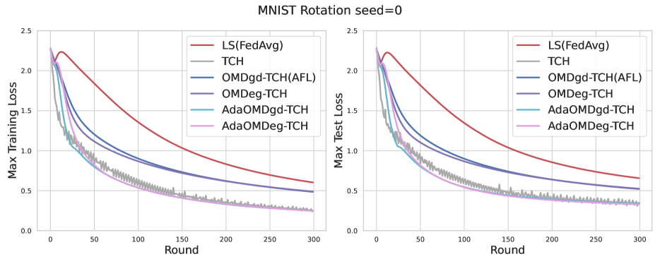
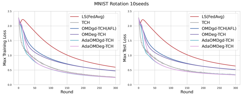
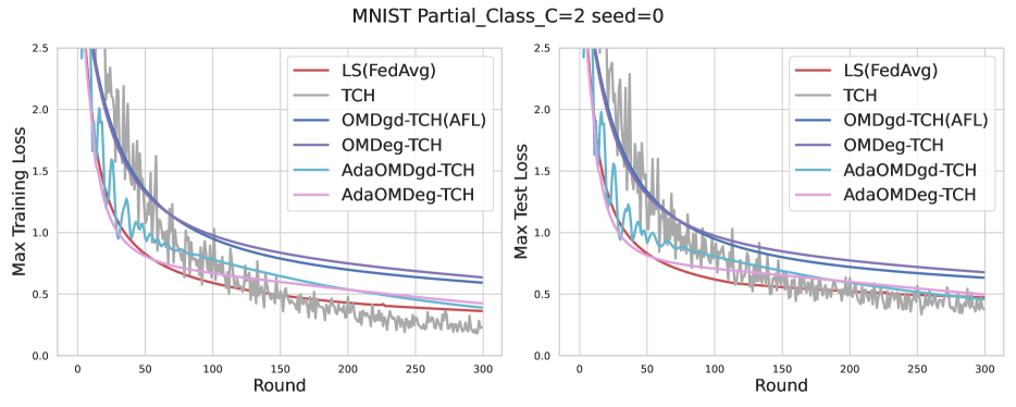
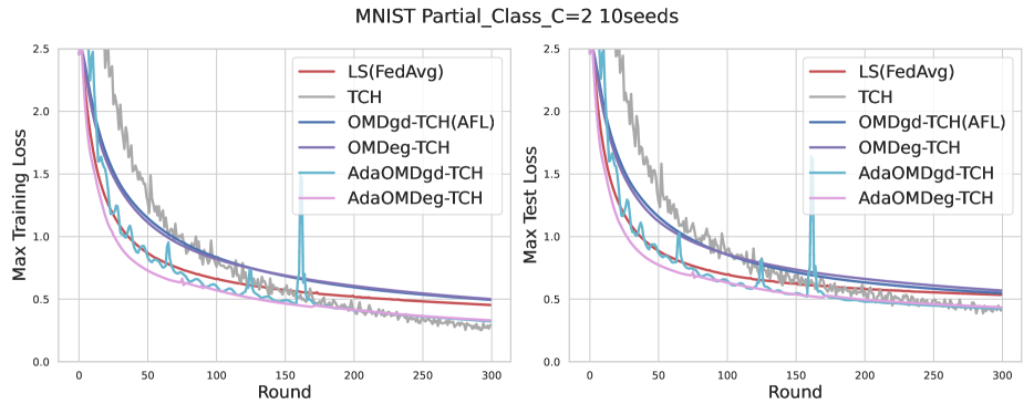
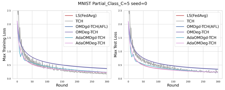
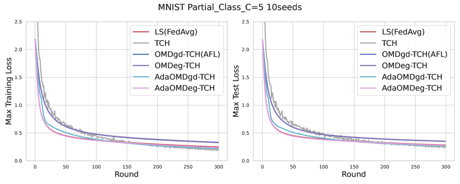
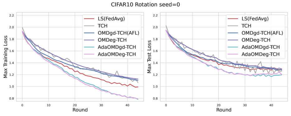
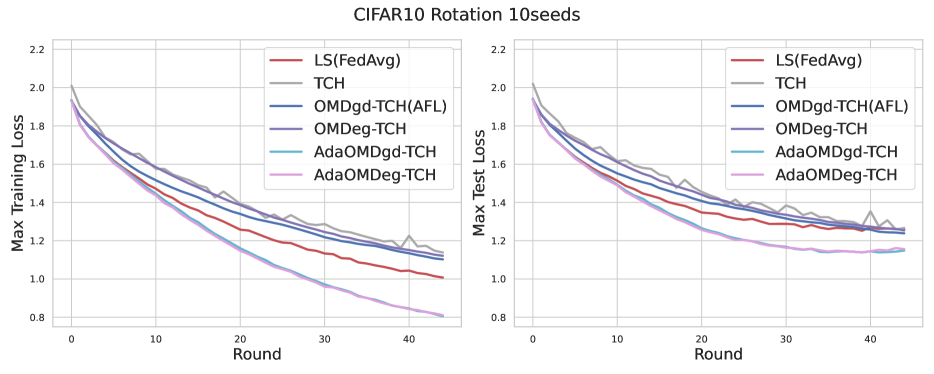
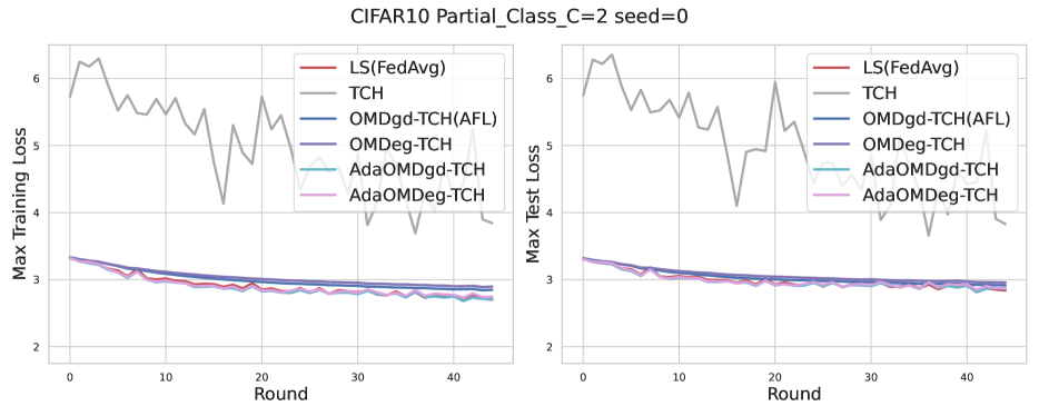
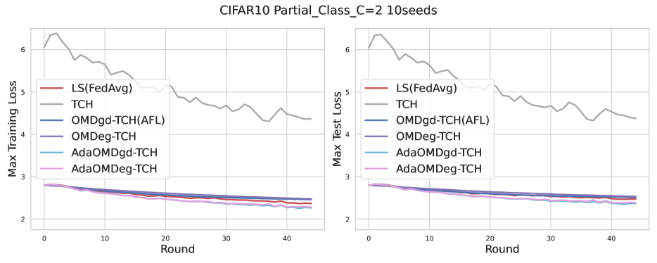
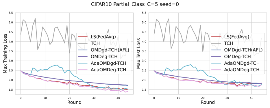
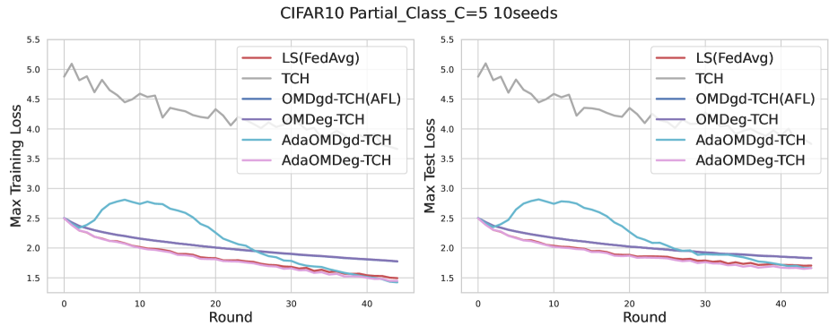
Figure 5: Training and Test Curves of Worst Client Loss.

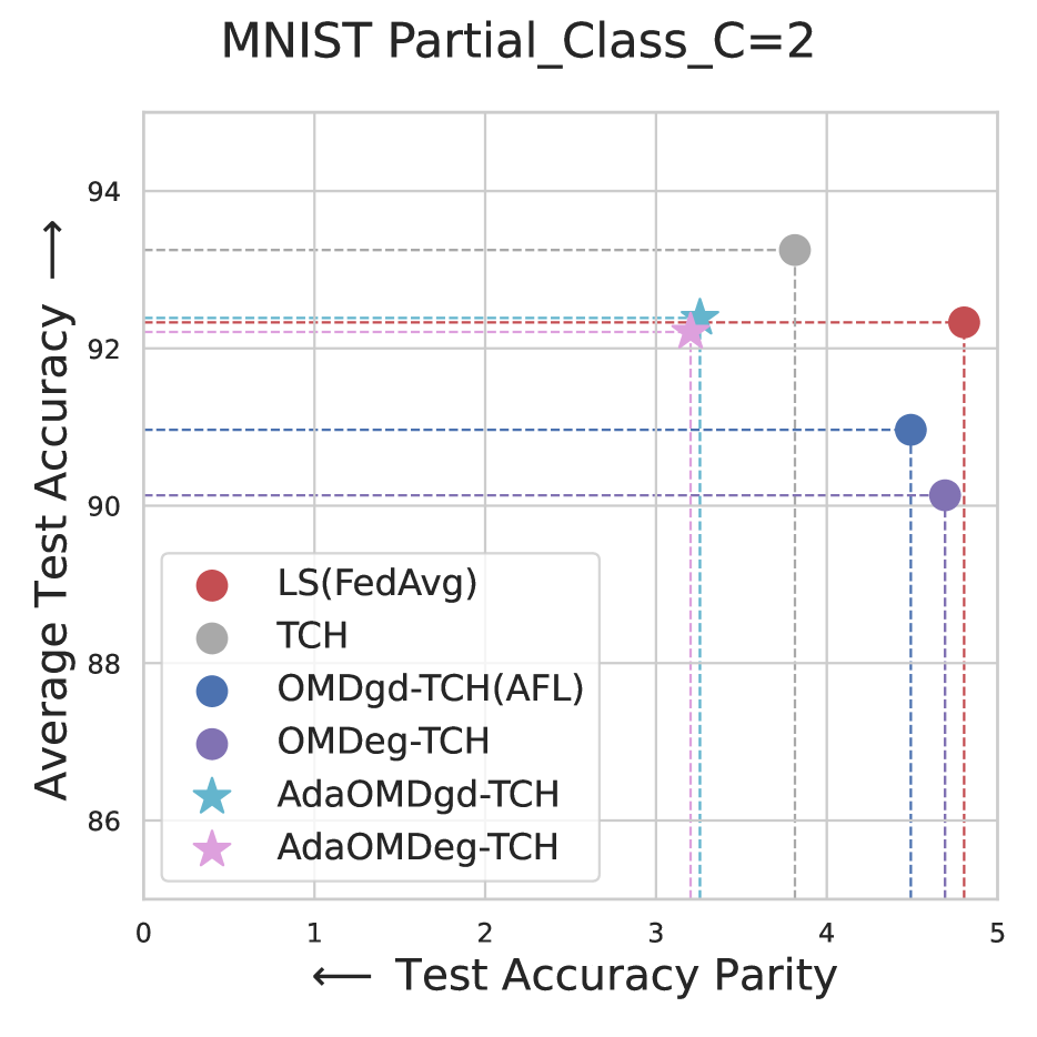
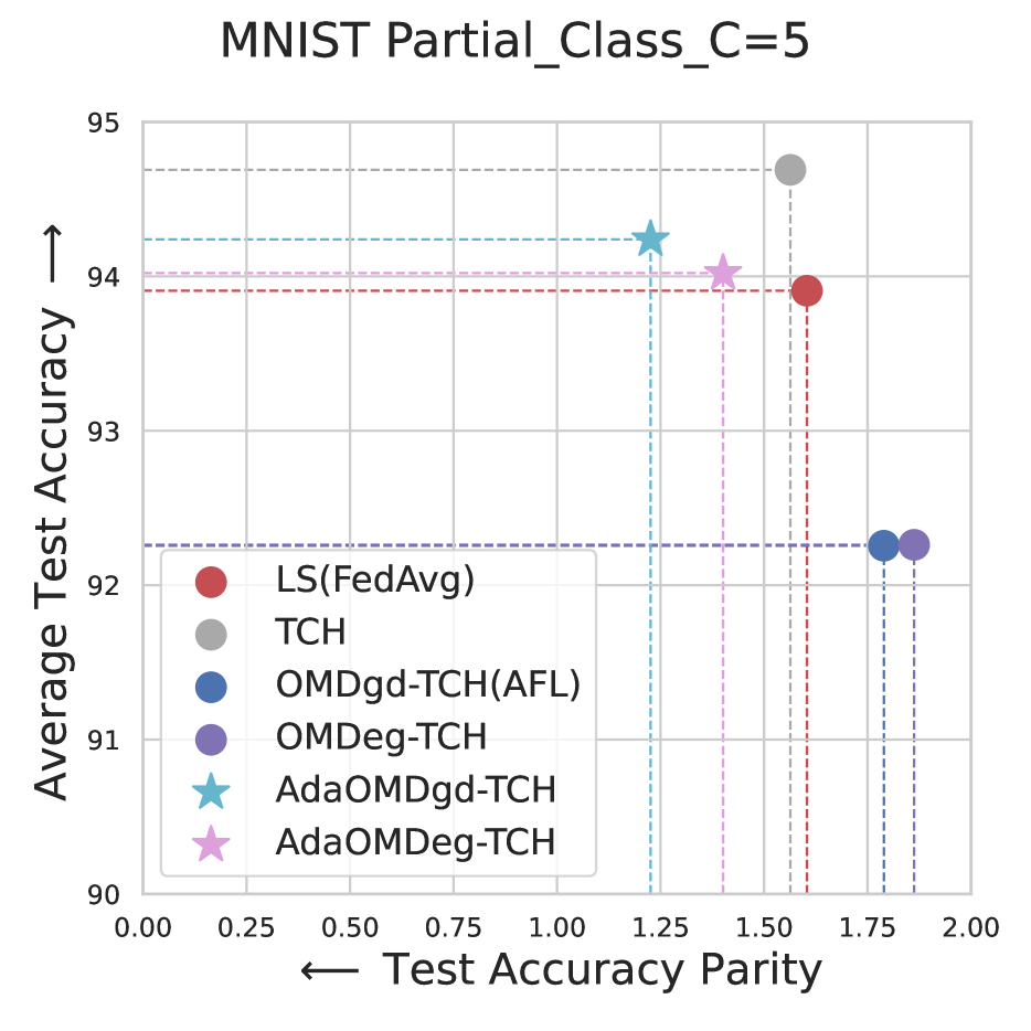
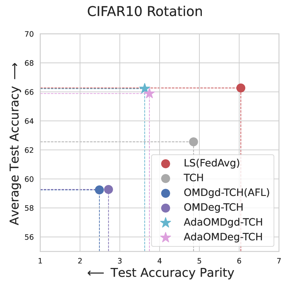
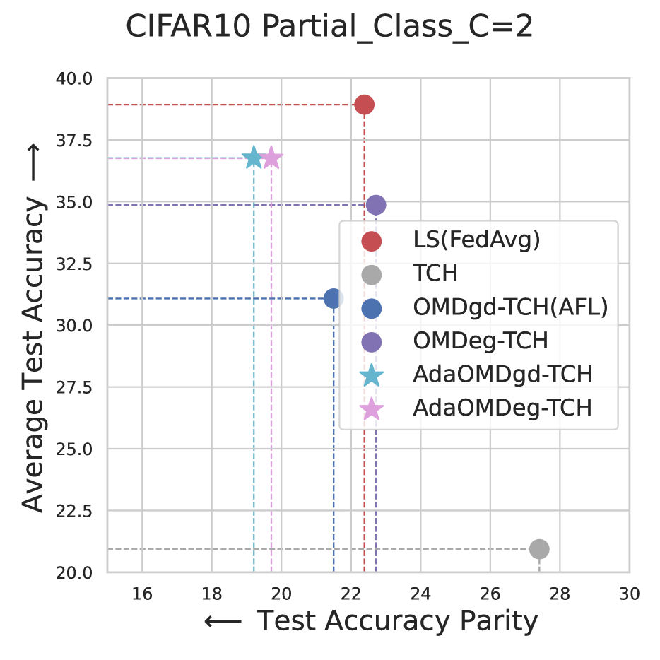
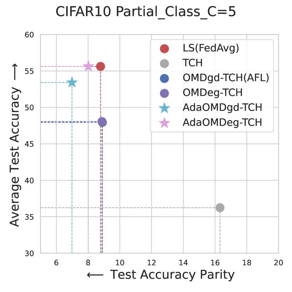
Figure 6: Scatter Plots of Average Accuracy and Accuracy Parity.

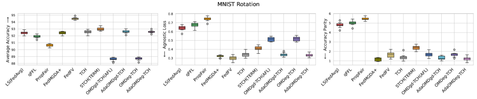
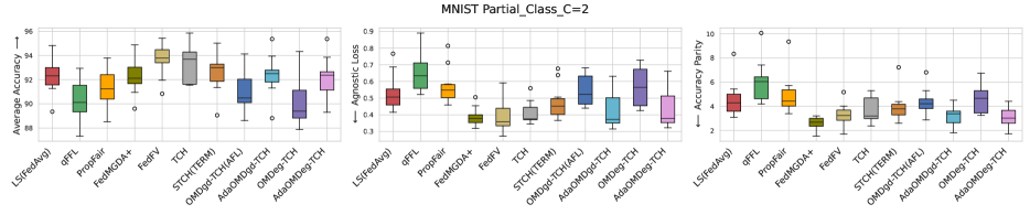
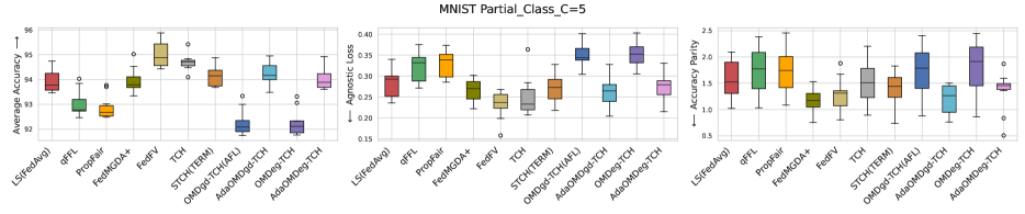
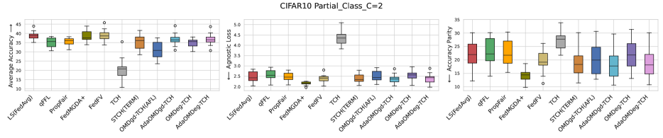
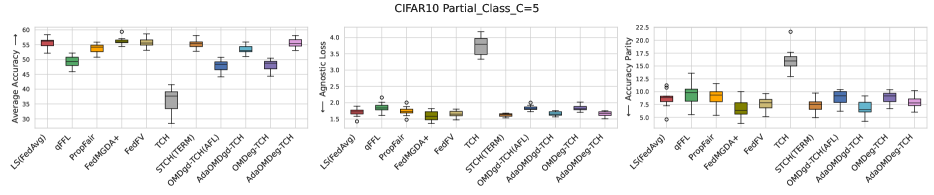
Figure 7: Boxplots of All Methods on Three Metrics.

References

• Azuma (1967) K. Azuma. Weighted sums of certain dependent random variables. Tohoku Mathematical Journal, Second Series, 19(3):357–367, 1967.
• Bowman Jr (1976) V. J. Bowman Jr. On the relationship of the tchebycheff norm and the efficient frontier of multiple-criteria objectives. In Multiple Criteria Decision Making, 1976.
• Boyd and Vandenberghe (2004a) S. Boyd and L. Vandenberghe. Convex optimization. Cambridge university press, 2004a.
• Boyd and Vandenberghe (2004b) S. Boyd and L. Vandenberghe. Convex optimization. Cambridge university press, 2004b.
• Caruana (1997) R. Caruana. Multitask learning. Machine Learning, 28, 1997.
• Cesa-Bianchi et al. (2004) N. Cesa-Bianchi, A. Conconi, and C. Gentile. On the generalization ability of on-line learning algorithms. IEEE Transactions on Information Theory, 50, 2004.
• Chen and Teboulle (1993) G. Chen and M. Teboulle. Convergence analysis of a proximal-like minimization algorithm using bregman functions. SIAM Journal on Optimization, 3(3):538–543, 1993.
• Choo and Atkins (1983) E. U. Choo and D. R. Atkins. Proper efficiency in nonconvex multicriteria programming. Mathematics of Operations Research, 8, 1983.
• Chu et al. (2022) W. Chu, C. Xie, B. Wang, L. Li, L. Yin, A. Nourian, H. Zhao, and B. Li. FOCUS: Fairness via agent-awareness for federated learning on heterogeneous data. arXiv preprint arXiv:2207.10265, 2022.
• Collins et al. (2021) L. Collins, H. Hassani, A. Mokhtari, and S. Shakkottai. Exploiting shared representations for personalized federated learning. In International conference on machine learning. PMLR, 2021.
• Das and Dennis (1997) I. Das and J. Dennis. A closer look at drawbacks of minimizing weighted sums of objectives for pareto set generation in multicriteria optimization problems. Structural Optimization, 14, 1997.
• Deb et al. (2002) K. Deb, A. Pratap, S. Agarwal, and T. Meyarivan. A fast and elitist multiobjective genetic algorithm: NSGA-II. IEEE Transactions on Evolutionary Computation, 6, 2002.
• Deng (2012) L. Deng. The mnist database of handwritten digit images for machine learning research [best of the web]. IEEE signal processing magazine, 29, 2012.
• Désidéri (2012) J.-A. Désidéri. Multiple-gradient descent algorithm (MGDA) for multiobjective optimization. Comptes Rendus Mathematique, 350, 2012.
• Ehrgott (2005) M. Ehrgott. Multicriteria optimization. Springer Science & Business Media, 2005.
• Fliege and Svaiter (2000) J. Fliege and B. F. Svaiter. Steepest descent methods for multicriteria optimization. Mathematical Methods of Operations Research, 51, 2000.
• Geoffrion (1967) A. M. Geoffrion. Solving bicriterion mathematical programs. Operations Research, 15, 1967.
• Ghosh et al. (2020) A. Ghosh, J. Chung, D. Yin, and K. Ramchandran. An efficient framework for clustered federated learning. Advances in Neural Information Processing Systems, 33, 2020.
• Haghtalab et al. (2023) N. Haghtalab, M. Jordan, and E. Zhao. A unifying perspective on multi-calibration: Game dynamics for multi-objective learning. In Advances in Neural Information Processing Systems, 2023.
• Hazan et al. (2016) E. Hazan et al. Introduction to online convex optimization. Foundations and Trends in Optimization, 2016.
• He et al. (2016) K. He, X. Zhang, S. Ren, and J. Sun. Deep residual learning for image recognition. In Proceedings of the IEEE conference on computer vision and pattern recognition, pages 770–778, 2016.
• He et al. (2024) Y. He, S. Zhou, G. Zhang, H. Yun, Y. Xu, B. Zeng, T. Chilimbi, and H. Zhao. Robust multi-task learning with excess risks. In Forty-first International Conference on Machine Learning, 2024.
• Hu et al. (2024) Y. Hu, R. Xian, Q. Wu, Q. Fan, L. Yin, and H. Zhao. Revisiting scalarization in multi-task learning: A theoretical perspective. Advances in Neural Information Processing Systems, 36, 2024.
• Hu et al. (2022a) Z. Hu, K. Shaloudegi, G. Zhang, and Y. Yu. Federated learning meets multi-objective optimization. IEEE Transactions on Network Science and Engineering, 2022a.
• Hu et al. (2022b) Z. Hu, K. Shaloudegi, G. Zhang, and Y. Yu. Federated learning meets multi-objective optimization. IEEE Transactions on Network Science and Engineering, 9, 2022b.
• Krizhevsky and Hinton (2009) A. Krizhevsky and G. Hinton. Learning multiple layers of features from tiny images. Technical report, University of Toronto, 2009.
• Li et al. (2019) T. Li, M. Sanjabi, A. Beirami, and V. Smith. Fair resource allocation in federated learning. arXiv preprint arXiv:1905.10497, 2019.
• Li et al. (2020) T. Li, A. Beirami, M. Sanjabi, and V. Smith. Tilted empirical risk minimization. arXiv preprint arXiv:2007.01162, 2020.
• Lin et al. (2019) X. Lin, H.-L. Zhen, Z. Li, Q.-F. Zhang, and S. Kwong. Pareto multi-task learning. In Advances in Neural Information Processing Systems, volume 32, 2019.
• Lin et al. (2024) X. Lin, X. Zhang, Z. Yang, F. Liu, Z. Wang, and Q. Zhang. Smooth tchebycheff scalarization for multi-objective optimization. In 41st International Conference on Machine Learning, 2024.
• Liu et al. (2021) B. Liu, X. Liu, X. Jin, P. Stone, and Q. Liu. Conflict-averse gradient descent for multi-task learning. Advances in Neural Information Processing Systems, 34:18878–18890, 2021.
• Mahapatra and Rajan (2020) D. Mahapatra and V. Rajan. Multi-task learning with user preferences: Gradient descent with controlled ascent in pareto optimization. In Proceedings of the 37th International Conference on Machine Learning, 2020.
• McMahan et al. (2017a) B. McMahan, E. Moore, D. Ramage, S. Hampson, and B. A. y. Arcas. Communication-efficient learning of deep networks from decentralized data. In Proceedings of the 20th International Conference on Artificial Intelligence and Statistics, 2017a.
• McMahan et al. (2017b) B. McMahan, E. Moore, D. Ramage, S. Hampson, and B. A. y Arcas. Communication-efficient learning of deep networks from decentralized data. In Artificial intelligence and statistics. PMLR, 2017b.
• Michel et al. (2021) P. Michel, S. Ruder, and D. Yogatama. Balancing average and worst-case accuracy in multitask learning. arXiv:2110.05838, 2021.
• Miettinen (1998) K. Miettinen. Nonlinear multiobjective optimization. International Series in Operations Research & Management Science, 12, 1998.
• Mohri et al. (2019) M. Mohri, G. Sivek, and A. T. Suresh. Agnostic federated learning. In Proceedings of the 36th International Conference on Machine Learning, 2019.
• Namkoong and Duchi (2016) H. Namkoong and J. C. Duchi. Stochastic gradient methods for distributionally robust optimization with f-divergences. In Advances in Neural Information Processing Systems, 2016.
• Navon et al. (2022) A. Navon, A. Shamsian, I. Achituve, H. Maron, K. Kawaguchi, G. Chechik, and E. Fetaya. Multi-task learning as a bargaining game. In Proceedings of the 39th International Conference on Machine Learning, 2022.
• Nemirovskij and Yudin (1983) A. S. Nemirovskij and D. B. Yudin. Problem complexity and method efficiency in optimization. Wiley-Interscience, 1983.
• Sagawa et al. (2020) S. Sagawa, P. W. Koh, T. B. Hashimoto, and P. Liang. Distributionally robust neural networks. In International Conference on Learning Representations, 2020.
• Schaffer (1985) J. D. Schaffer. Multiple objective optimization with vector evaluated genetic algorithms. In Proceedings of the First International Conference on Genetic Algortihms, 1985.
• Sener and Koltun (2018) O. Sener and V. Koltun. Multi-task learning as multi-objective optimization. In Advances in Neural Information Processing Systems, volume 31, 2018.
• Senushkin et al. (2023) D. Senushkin, N. Patakin, A. Kuznetsov, and A. Konushin. Independent component alignment for multi-task learning. In Proceedings of the IEEE/CVF Conference on Computer Vision and Pattern Recognition, 2023.
• Van Veldhuizen and Lamont (1999) D. A. Van Veldhuizen and G. B. Lamont. Multiobjective evolutionary algorithm test suites. In Proceedings of the 1999 ACM symposium on Applied computing, 1999.
• Wang et al. (2021) Z. Wang, X. Fan, J. Qi, C. Wen, C. Wang, and R. Yu. Federated learning with fair averaging. arXiv preprint arXiv:2104.14937, 2021.
• Xie et al. (2021) Y. Xie, C. Shi, H. Zhou, Y. Yang, W. Zhang, Y. Yu, and L. Li. Mars: Markov molecular sampling for multi-objective drug discovery. In International Conference on Learning Representations, 2021.
• Yu et al. (2020) T. Yu, S. Kumar, A. Gupta, S. Levine, K. Hausman, and C. Finn. Gradient surgery for multi-task learning. Advances in Neural Information Processing Systems, 33:5824–5836, 2020.
• Zhang et al. (2022) G. Zhang, S. Malekmohammadi, X. Chen, and Y. Yu. Proportional fairness in federated learning. arXiv preprint arXiv:2202.01666, 2022.
• Zhang and Li (2007) Q. Zhang and H. Li. MOEA/D: A multiobjective evolutionary algorithm based on decomposition. IEEE Transactions on Evolutionary Computation, 11, 2007.
• Zhang et al. (2024a) X. Zhang, X. Lin, and Q. Zhang. PMGDA: A preference-based multiple gradient descent algorithm. IEEE Transactions on Emerging Topics in Computational Intelligence, 2024a.
• Zhang et al. (2024b) X. Zhang, L. Zhao, Y. Yu, X. Lin, Y. Chen, H. Zhao, and Q. Zhang. Libmoon: A gradient-based multiobjective optimization library in pytorch. Advances in Neural Information Processing Systems, 2024b.
• Zhang et al. (2024c) Z. Zhang, W. Zhan, Y. Chen, S. S. Du, and J. D. Lee. Optimal multi-distribution learning. In The Thirty Seventh Annual Conference on Learning Theory, 2024c.
• Zinkevich (2003) M. Zinkevich. Online convex programming and generalized infinitesimal gradient ascent. In Proceedings of the 20th international conference on machine learning (icml-03), 2003.