Néel Spin-Orbit Torque in Antiferromagnetic Quantum Spin and Anomalous Hall Insulators

Abstract

Interplay between magnetic ordering and topological electrons not only enables new topological phases but also underpins electrical control of magnetism. Here we extend the Kane-Mele model to include the exchange coupling to a collinear background antiferromagnetic (AFM) order, which can describe transition metal trichalcogenides. Owing to the spin-orbit coupling and staggered on-site potential, the system could exhibit the quantum anomalous Hall and quantum spin Hall effects in the absence of a net magnetization. Besides the chiral edge states, these topological phases support a staggered Edelstein effect through which an applied electric field can generate opposite non-equilibrium spins on the two AFM sublattices, realizing the Néel-type spin-orbit torque (NSOT). Contrary to known NSOTs in AFM metals driven by conduction currents, our NSOT arises from pure adiabatic currents devoid of Joule heating, while being a bulk effect not carried by the edge currents. By virtue of the NSOT, the electric field of a microwave can drive the AFM dynamics with a remarkably high efficiency. Compared to the ordinary AFM resonance driven by the magnetic field, the new mechanism can enhance the resonance amplitude by more than one order of magnitude and the absorption rate of the microwave power by over two orders of magnitude. Our findings unravel an incredible way to exploit AFM topological phases to achieve ultrafast magnetic dynamics.

I Introduction

Harnessing topological materials to manipulate magnetism and magnetic dynamics has opened unique opportunities for energy-efficient spintronics. Recently, a new twist in this direction is inspired by the study of intrinsic magnetic topological insulators (iMTIs), in which topological electrons are highly entangled with the magnetic states [1, 2, 3, 4, 5, 6, 7, 8, 9, 10, 11]. Thanks to the synergy of electronic and magnetic degrees of freedom, an iMTI could be operated simultaneously as an electric actuator and a magnetic oscillator without the aid of foreign systems [12], forming a mono-structural setup to achieve spintronic functionalities that would otherwise rely on engineered heterostructures.

Meanwhile, because of the insulating nature of iMTIs, the spin-orbit torque (SOT) and the associated internal spin-transfer processes are not driven by Ohm’s currents; instead, they arise from the voltage-induced adiabatic currents carried by topological electrons in the valence band. Because adiabatic currents do not incur Joule heating, they can convert 100% of the input electric power into magnetic dynamics [13], leveraging an unprecedented boost of energy efficiency compared to established solutions. While we have recently demonstrated such lossless SOT and its ensuing physical effects in a widely recognized iMTI – MnBi₂Te₄ of a few layer thick [12], the obtained results only revealed the tip of an enormous unexplored iceberg.

In particular, we identify five outstanding questions beyond what could be answered by the iMTI family of materials. First, what non-trivial topological phases are compatible with a given magnetic order, especially the compensated antiferromagnetic (AFM) state? Second, can these topological phases afford the lossless SOT? Third, will the SOT prevail down to the monolayer limit? Fourth, will a strong Néel-type SOT (NSOT), i.e., contrasting fields acting different sublattices, be supported by symmetry? Finally, what are the dynamical implications of the NSOT in a chosen material? The known case of MnBi₂Te₄ only provides us with limited information. For instance, the material becomes a compensated AFM (ferromagnetic) system only if there are even (odd) number of layers, which corresponds to an axion (quantum anomalous Hall) insulator. In either phase, however, the SOT vanishes identically in the monolayer limit while the NSOT is forbidden by symmetry [12, 14] within the linear response regime.

To answer these open questions, we investigate a new scenario of insulating magnets which could potentially host topological electrons on their own. While transition-metal trichalcogenides (TMTs) such as MnPS₃ generally escape the radar of topological materials, they can be effectively described by an extended Kane-Mele model [15, 16] including the exchange coupling of electrons to a uniform AFM order. Depending on the spin-orbit coupling and a staggered potential, a monolayer TMT could exhibit the quantum anomalous Hall (QAH) effect [17, 18] and the quantum spin Hall (QSH) effect [19, 20], both of which turn out to be compatible with a fully compensated collinear AFM order. Moreover, we find that both the QAH and QSH phases support a staggered Edelstein effect, by which an applied electric field can generate opposite non-equilibrium spins acting on different sublattice magnetic moments, realizing the desired NSOT without incurring Joule heating as conduction electrons are eliminated. Similar to the SOT previously claimed in iMTIs [12], the NSOT studied in this paper is determined by the Berry curvature residing in the parameter space spanned by the crystal momenta and the magnetic orientation, which is subtly related to but cannot be fully characterized by the band topology.

To demonstrate the physical significance of our prediction, we study the NSOT-induced AFM resonance and benchmark the result against an ordinary AFM resonance. Remarkably, the NSOT renders the electric field of a microwave the dominant driving force, which overwhelms the direct coupling to the magnetic field, thus enhancing the AFM resonance amplitude by more than one order of magnitude. The high efficiency of this counter-intuitive electric field-driven AFM resonance is quantified by the dynamical susceptibility. Our findings not only identify the exciting possibility of achieving NSOT in 2D magnets, but also unravel a unique mechanism to generate ultrafast AFM dynamics devoid of Joule heating by exploiting magnetic topological materials.

Figure 1: Honeycomb lattice with G-type AFM order (red and blue arrows). The wavy potential well represents the staggered potential on A and B sublattices. The intrinsic SOC and Rashba SOC introduce extra phases in the nearest neighbor (white dashed line) and next nearest neighbor hopping (black dashed line), respectively. The coordinates axis are shown on the left.

II Formalism

We extend the Kane-Mele model by including a collinear AFM order which is exchange coupled to the electrons on a honeycomb lattice. As illustrated in Fig.1, the magnetic moments on the A and B sublattices are oppositely aligned and pointing perpendicular to the plane. The conceived system is characterized by an effective tight-binding Hamiltonian

$$H=t\sum_{\langle i,j\rangle}c_{i}^{\dagger}c_{j}+i\lambda_{soc}\sum_{\langle\langle i,j\rangle\rangle}\nu_{ij}c_{i}^{\dagger}s_{z}c_{j}+i\lambda_{R}\sum_{\langle i,j\rangle}c_{i}^{\dagger}(\bm{s}\times\hat{\bm{d}}_{ij})_{z}c_{j}+\lambda_{\nu}\sum_{i}c_{i}^{\dagger}\xi_{i}c_{i}+\lambda_{ex}\sum_{i}c_{i}^{\dagger}(\bm{m}_{i}\cdot\bm{s})c_{i},$$ (1)

where $c_{i}^{\dagger}(c_{i})$ is the electron creation (annihilation) operator on site $i$ with the spin index omitted for succinctness. In Eq. (1), the first term represents the nearest neighbor hopping. The second term is the intrinsic spin-orbit coupling (SOC) which affects the next-nearest neighbor hopping, where $\nu_{ij}=2/\sqrt{3}(\hat{\bm{d}}_{1}\times\hat{\bm{d}}_{2})_{z}=\pm 1$ with $\hat{\bm{d}}_{1}$ and $\hat{\bm{d}}_{2}$ being the two unit vectors along the $120^{\circ}$ bonds connecting $i$ and $j$. The third term is the Rashba SOC arising from the broken inversion symmetry, where $\hat{\bm{d}}_{ij}$ is the unit vector connecting the nearest-neighboring sites $i$ and $j$, and $\bm{s}$ is the vector of Pauli matrices for the spin degree of freedom. The fourth term is the staggered potential where $\xi_{i}=\pm 1$ flips sign on the A and B sublattices as shown in the Fig. 1, breaking the $C_{2}$ symmetry about the $x$ axis. The last term represents the exchange coupling between the electrons and the local magnetic moments, where $\bm{m}_{i}=\pm\bm{z}$ is the unit magnetic vector on site $i$.

III Topological Phases

If the exchange coupling $\lambda_{ex}$ vanishes, the Hamiltonian preserves the time-reversal symmetry (TRS). Then for a sufficiently large $\lambda_{soc}$, the system can exhibit the QSH phase characterized by a $Z_{2}$ number. Now, the TRS is broken for finite $\lambda_{ex}$, rendering the $Z_{2}$ number ill-defined. Since the total Chern number $C$ also vanishes, we must resort to the spin Chern number $C_{s}=(C_{\uparrow}-C_{\downarrow})/2$  [21, 22] to distinguish such a system from a normal insulator (NI) with trivial band topology. To ensure a proper quantization of the topological invariant, we impose an upper limit of $0.1t$ for the values of $\lambda_{soc}$, $\lambda_{R}$, $\lambda_{ex}$ and $\lambda_{\nu}$ so as to maintain a global band gap.

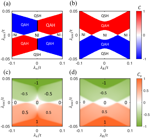
Figure 2: The phase diagram for Chern number [(a) and (b)] and spin Chern number [(c) and (d)] with respect to intrinsic SOC strength $\lambda_{soc}$ for different staggered potential and Rashba SOC strength $\lambda_{R}$. In (a) and (c), $\lambda_{R}$ is fixed to be $0.05t$. In (b) and (d), $\lambda_{\nu}$ is fixed to be $0.05t$. In all cases, $\lambda_{ex}=0.1t$.

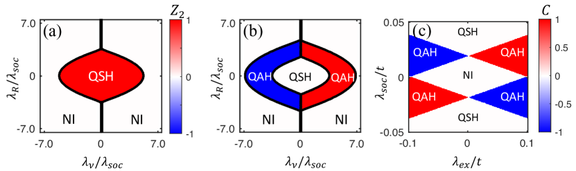
Figure S1: (a) Phase diagram of the $Z_{2}$ number in the absence of the AFM order (original Kane-Mele model) for $\lambda_{soc}=0.06t$ and $\lambda_{ex}=0$ (b) Phase diagram of the Chern number in the presence of the AFM order for $\lambda_{soc}=0.06t$ and $\lambda_{ex}=0.1t$. (c) Phase diagram of the Chern number for different exchange coupling strengths $\lambda_{ex}$ and intrinsic SOC $\lambda_{soc}$ for $\lambda_{\nu}=\lambda_{R}=0.05t$

We first calculate the total Chern number $C$ by navigating the values of $\lambda_{soc}$, $\lambda_{\nu}$ and $\lambda_{R}$, which is plotted in Fig. 2(a) and (b). We find three distinct phases on these diagrams, where the QSH state only appears at large $\lambda_{soc}$. At $\lambda_{\nu}=0$, the threshold of QSH is about $\lambda_{soc}=\pm 0.03t$. Two observations are in order. First, the QAH state requires a nonzero staggered potential $\lambda_{\nu}$ while the QSH state does not. To enable the QAH phase in a collinear AFM background, it is essential to break the sublattice exchange symmetry [23, 24, 25] on top of other symmetry requirements, and the staggered potential is a common way of realization. Second, the Chern number flips sign when either $\lambda_{\nu}$ or $\lambda_{soc}$ flips sign, but it remains the same sign regardless of $\lambda_{R}$. In Fig. S1, we also provide the phase diagrams for other combinations of parameters (e.g., $\lambda_{soc}$ and $\lambda_{ex}$). We conclude that the sign of the total Chern number is $\mathrm{sign}[C]=\mathrm{sign}[\lambda_{soc}]\mathrm{sign}[\lambda_{\nu}]\mathrm{sign}[\lambda_{ex}]$.

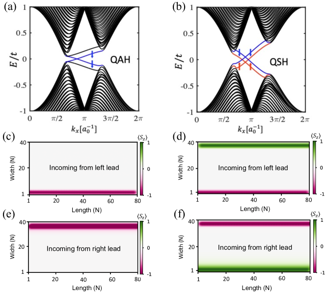
Figure 3: Band structure of a periodic nano-ribbon with finite width $N=40$ for (a) $\lambda_{soc}=0.02t$ and (b) $\lambda_{soc}=0.05t$. In both cases, we set $4\lambda_{R}=2\lambda_{\nu}=\lambda_{ex}=0.1t$. The edge states lying in the bulk gap are colored blue or red depending on the spin polarization. Spatial distribution of the normalized spin-resolved edge electron transport in a finite sample (width$\times$length = $40\times 80$) for the QAH state [(c) and (e)] and the QSH state [(d) and (f)].

To further understand the physical meaning of different phases, we plot in Figs. 2(c) and (d) the phase diagrams of the spin Chern number $C_{s}$, corresponding to Figs. 2(a) and (b), respectively. As expected, $C_{s}$ in the QSH state is quantized to be $\pm 1$. In the QAH state, however, $C_{s}$ is quantized to be $\pm 0.5$, which indicates that the chiral edge electrons only carry one spin species. It is important to note that the spin Chern number near the phase boundaries is not exactly quantized, because the spin is not a strictly conserved quantity in the presence of a finite Rashba SOC. Concerning the sign flip of $C_{s}$, we observe a quite different pattern as compared to $C$. For example, $C_{s}$ is even in $\lambda_{v}$ while being odd in $\lambda_{soc}$. This can be understood by the definition of spin currents: if the spin polarization and the flowing direction both flip sign, a spin current will remain unchanged.

To confirm the system topology from a real-space perspective, we truncate our periodic Hamiltonian (1) in the $y$ direction with a width of $N=40$ unit cells and calculate the band structure of such one dimensional nano-strip. From Figure 3(a) shows that two chiral edge states with opposite group velocities emerge in the bulk gap at $\lambda_{soc}=0.02t$, which corresponds to the QAH state. We further truncate the nano-strip in the $x$ direction with $N=80$ unit cells as the scattering region. Figures 3(c) and (e) show the spin-resolved distribution of the scattering states from the left and right lead with energy fixed in the bulk gap, where the right-propagating (left-propagating) current mainly locates at the lower (upper) edge. Additionally, these scattering states both have a spin-down polarization, consistent with the physical picture of the QAH effect. As $\lambda_{soc}$ is further increased to $0.05t$, the system exhibits two pairs of chiral edge states in the bulk gap with opposite group velocities, as shown in Fig. 3(b). We again plot the corresponding spin-resolved distribution of the scattering states in Figs. 3(d) and (f). Distinct from the QAH case, here both the right- and left-propagating currents appear at each edge. Moreover, the states on opposite edges exhibit opposite spin polarization, consistent with the physical picture of the QSH effect.

IV Néel-type spin-orbit torque

Having obtained the band topology with broken TRS introduced by the AFM order, we are in a good position to explore the interplay between electron transport and magnetic dynamics. For insulating systems where the ordinary spin Hall effect is suppressed, applying an (in-plane) electric field $\bm{E}$ can directly generate non-equilibrium spin accumulation through the Edelstein effect [26]. The induced spin accumulation can in turn excite magnetic dynamics through the SOT [27, 28, 29, 30]. In our context, it is important to discern different AFM sublattices in the non-equilibrium spin generation. While the average component $\delta\bm{S}=(\delta\bm{S}^{A}+\delta\bm{S}^{B})/2$ (due to the Edelstein effect) leads to the ordinary SOT, the contrasting component $\delta\bm{N}=(\delta\bm{S}^{A}-\delta\bm{S}^{B})/2$ (due to the staggered Edelstein effect) leads to the NSOT [31]. As we consider insulating magnets where the Fermi energy $\varepsilon_{F}$ lies in the bulk gap, $\delta\bm{S}$ and $\delta\bm{N}$ only involve the Fermi-sea contribution. Within the linear response regime, we can express the contrasting spin accumulation as

$$\delta\bm{N}=\frac{e\hbar^{2}}{2}\sum_{\epsilon_{n}<\varepsilon_{F}<\epsilon_{m}}\int_{\mathrm{BZ}}\frac{dk^{2}}{(2\pi)^{2}}{\rm Im}\left[\bra{n}\bm{s}\otimes\tau_{3}\ket{m}\bra{m}\bm{v}\cdot\bm{E}\ket{n}\right]\frac{(\epsilon_{n}-\epsilon_{m})^{2}-\Gamma^{2}}{[(\epsilon_{n}-\epsilon_{m})^{2}+\Gamma^{2}]^{2}},$$ (2)

where $\bm{v}$ is the velocity operator and $\Gamma$ is the energy broadening due to disorder. The average spin accumulation $\delta\bm{S}$ follows a similar formula with the pseudo-spin Pauli matrix (acting on the sublattices) $\tau_{3}$ replaced by the identity matrix. Unlike the Fermi-level contribution, here $\delta\bm{N}$ does not diverge even in the clean limit $\Gamma\rightarrow 0$ where Eq. (2) reduces to a formula similar to the spin Chern number [see Eq. (7)]. In the following, we will take representative values for the exchange interaction $\lambda_{ex}=0.1t=100\ \mathrm{meV}$ and for the band broadening $\Gamma=20\ \mathrm{meV}$.

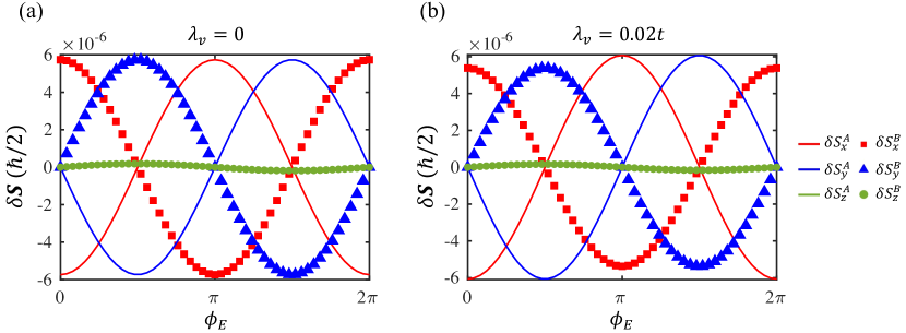
Figure S4: The non-equilibrium spin accumulation $\delta\bm{S}$ per square nanometer as a function of the in-plane azimuthal angle $\phi_{E}$ of the applied electric field when the staggered potential $\lambda_{v}$ is (a) turned off; and (b) turned on. Parameters : $\lambda_{R}=\lambda_{soc}=0.05$, $\Gamma=20$ meV, and $E_{x}=1\ \mathrm{V/\mu m}$.

Without sacrificing generality, we set the $\bm{E}$ field in the $x$ direction and calculate the non-equilibrium spin accumulation on each sublattice: $\delta{\bm{S}}^{A}=(\delta{\bm{S}}+\delta{\bm{N}})/2$ and $\delta{\bm{S}}^{B}=(\delta{\bm{S}}-\delta{\bm{N}})/2$. Figure 4(a) and (b) plot $\delta S^{A}_{x}$ and $\delta S^{B}_{x}$ as functions of $\lambda_{soc}$ and $\lambda_{R}$, while the $y$ and $z$ components are found to be zero. Remarkably, we find that $\delta S^{A}_{x}$ and $\delta S^{B}_{x}$ are exactly opposite to each other so long as $\lambda_{\nu}=0$, meaning that only the NSOT exists whereas the SOT vanishes (i.e., $\delta\bm{S}=0$). As a consistency check, the way $\delta\bm{S}^{A(B)}$ varies over the direction of $\bm{E}$ is shown in Fig. S4, where the contrasting feature $\delta{S}^{A}_{x(y)}=-\delta{S}^{B}_{x(y)}$ persists.

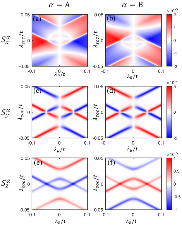
Figure S2: Non-equilibrium spin accumulation in unit of $\hbar/2$ per unit cell for each sublattice in different directions. $S^{\alpha}_{y}$ and $S^{\alpha}_{z}$ are nonzero only in the vicinity of the phase boundaries. Parameters: $E_{x}=1\ \rm V/\mu m$, $2\lambda_{\nu}=\lambda_{ex}=0.1t=100\ \mathrm{meV}$, and $\Gamma=20$meV.

A non-zero $\lambda_{\nu}$ would render $|\delta S^{A}_{x}|\neq|\delta S^{B}_{x}|$ owing to the introduction of staggered potentials on the sublattices (see Fig. S2), which leads to a finite $\delta\bm{S}$ on top of the $\delta\bm{N}$, hence inducing a nonzero SOT besides the NSOT. Figure 4(c) and (d) schematically show the difference between the SOT and NSOT, driven by $\delta{\bm{S}}^{A}=\delta{\bm{S}}^{B}$ and $\delta{\bm{S}}^{A}=-\delta{\bm{S}}^{B}$, respectively. In the clean limit $\Gamma\rightarrow 0$, the spin accumulation on each sublattice is directly related to the Berry curvature residing in the mixed space of crystal momentum and magnetization [13]:

$$\delta S_{\nu}^{A(B)}=\frac{e\hbar}{2\lambda_{ex}}E_{\mu}\left\langle\Omega_{\mu\nu}^{km^{A(B)}}\right\rangle,$$ (3)

where $\langle\cdots\rangle=V_{\rm uc}/(2\pi)^{2}\sum_{n}\int{\rm d}^{2}kf[\varepsilon_{n}(\bm{k})](\cdots)$ denotes the average over the first Brillouin zone with $V_{\rm uc}$ the unit cell volume (area) and the $f$ the Fermi distribution. For $\lambda_{V}=0$, the Berry curvature assumes a staggered pattern $\Omega_{\mu\nu}^{km^{A}}=-\Omega_{\mu\nu}^{km^{B}}$ thus $\delta{\bm{S}}^{A}=-\delta{\bm{S}}^{B}$.

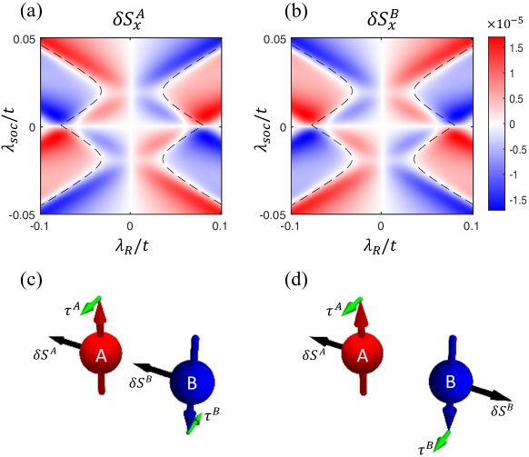
Figure 4: (a) and (b): Non-equilibrium spin accumulation per unit cell (in units of $\hbar/2$) for each sublattice for $E_{x}=1\ \rm V/\mu m$ and $\lambda_{\nu}=0$. The dashed lines mark where the global band gap is reduced to $1$ meV with an increasing $|\lambda_{R}|$. Illustrative comparison between: (c) ordinary SOT induced by a uniform spin accumulation $\delta\bm{S}$, and (d) NSOT induced by a contrasting spin accumulation $\delta\bm{N}$.

In the phase diagram, the dashed lines mark where the global band gap reduces to $1$ meV. For a large $|\lambda_{R}|$ beyond these boundaries, the global band gap will be smaller than $1$ meV, making it less realistic to restrict the Fermi level to the band gap over the entire Brillouin zone. In other words, we should focus on the central region of Fig. 4(a) and (b) enclosed by the dashed lines in order to safely ignore the Fermi-surface contribution to $\delta\bm{S}^{A(B)}$.

The NSOT is known for being able to switch the Néel order $\bm{n}=(\bm{m}^{A}-\bm{m}^{B})/2$ in non-centrosymmetric AFM metals [32, 33, 34, 35]. But all known scenarios are current-induced NSOT, which suffers from significant Joule heating. By contrast, our predicted NSOT is in principle free of dissipation because it is mediated by the adiabatic motions of valence electrons, incurring no Ohm’s current as no conduction electrons are involved in the generation of spin torques. The adiabatic origin of the NSOT is also reflected by its Berry-curvature origin discussed above.

V Electric Field-Driven AFM resonance

To demonstrate the dynamical consequences of the predicted NSOT, we now study the AFM resonance driven by an AC electric field. In terms of the unit vectors of the sublattice magnetic moments, the governing Landau-Lifshitz-Gilbert (LLG) equations are:

$$\bm{\dot{m}}^{A} =\gamma\left[-\mathcal{H}_{J}\bm{m}^{B}+\mathcal{H}_{\parallel}(\bm{e}_{\parallel}\cdot\bm{m}^{A})\bm{e}_{\parallel}+\bm{H}_{0}+\bm{h}^{A}_{D}\right]\times\bm{m}^{A}+\alpha_{0}\bm{m}^{A}\times\bm{\dot{m}}^{A}$$

$$\bm{\dot{m}}^{B} =\gamma\left[-\mathcal{H}_{J}\bm{m}^{A}+\mathcal{H}_{\parallel}(\bm{e}_{\parallel}\cdot\bm{m}^{B})\bm{e}_{\parallel}+\bm{H}_{0}+\bm{h}^{B}_{D}\right]\times\bm{m}^{B}+\alpha_{0}\bm{m}^{B}\times\bm{\dot{m}}^{B},$$ (4)

where $\gamma>0$ is the gyromagnetic ratio, $\mathcal{H}_{J}$ is the AFM exchange field (summed over all nearest neighbors), $\mathcal{H}_{\parallel}$ is the anisotropy field for the easy axis $\bm{e}_{\parallel}$, $\bm{H}_{0}$ is the external static field, and $\alpha_{0}$ is the Gilbert damping constant. For simplicity, let $\bm{e}_{\parallel}$ be the $z$ axis and $\bm{H}_{0}$ be applied along $\bm{e}_{\parallel}$, lifting the degeneracy of the AFM resonance modes.

Under a microwave irradiation, the oscillating driving field $\bm{h}_{D}^{A(B)}$ can arise either directly from the magnetic field $\bm{h}_{\rm rf}$ or indirectly from the NSOT field $\bm{h}_{\rm{NS}}^{A(B)}=-2\lambda_{ex}\delta\bm{S}^{A(B)}/\hbar m_{s}$ produced by the electric field $\bm{E}_{\rm{rf}}$ with $m_{s}$ being the sublattice magnetic moment. Of the two mechanisms, $\bm{h}_{\rm rf}$ ($\bm{h}_{\rm{NS}}$) is perpendicular (parallel) to $\bm{E}_{\rm{rf}}$ and is the same (opposite) on each sublattice. Based on Maxwell’s equations, a microwave with $|\bm{E}_{\rm{rf}}|=1\ \rm V/\mu m$ has a magnetic field $|\bm{h}_{\rm rf}|=33$ Gauss. The same electric field can generate a maximum non-equilibrium spin of $0.85\times 10^{-5}$ $\hbar$ per sublattice according to Fig. 4, which converts to an effective NSOT field $|\bm{h}_{\rm{NS}}|=59$ Gauss for $m_{s}=5\mu_{B}$. While we are not able to locate a specific material on the phase diagram Fig. 4, it is instructive to chose a point where $|\bm{h}_{\rm rf}|=|\bm{h}_{\rm{NS}}|$, so we can determine how their distinct symmetry (uniform $\bm{h}_{\rm rf}$ versus opposite $\bm{h}_{\rm{NS}}$ on the two sublattices) could lead to dramatically different microwave absorptions with the onset of AFM resonance.

To this end, we focus on the point at $\lambda_{soc}=0.05t$, $\lambda_{R}=0.072t$, and $\lambda_{\nu}=0$, which lies in the QSH phase. Here, an electric field of $0.5\rm V/\mu m$ will produce a staggered spin accumulation $\delta S^{A}_{x}=-\delta S^{B}_{x}=-2.4\times 10^{-6}\hbar$ per unit cell (about 56% of the maximum capacity on the phase diagram), which corresponds to $h_{\rm NS}=16.5$ G, matching the real magnetic field $h_{\rm rf}$ of the same electromagnetic wave. On the material side, we take $m_{s}=5\mu_{B}$, $\mathcal{H}_{J}=35$ T and $\mathcal{H}_{\parallel}=0.16$ T, fairly close to the measured values in $\mathrm{MnPS_{3}}$ [36] which exhibits persisting AFM order in the 2D limit [37, 38]. We then consider a linearly polarized microwave incident from the $y$ direction with either $\bm{h}_{\rm rf}$ or $\bm{E}_{\rm rf}$ (hence the $\bm{h}_{\rm NS}$), but not both, parallel to the $x$ axis, as illustrated in Fig. 5(a) and (b), respectively. Under the device geometry in Fig. 5(a) [Fig. 5(b)], the electric field $\bm{E}_{\rm rf}$ (magnetic field $\bm{h}_{\rm rf}$) is collinear with the magnetic moments so that only $\bm{h}_{\rm rf}$ ($\bm{E}_{\rm rf}$) drives the AFM dynamics, separating the NSOT-induced resonance from the ordinary AFM resonance.

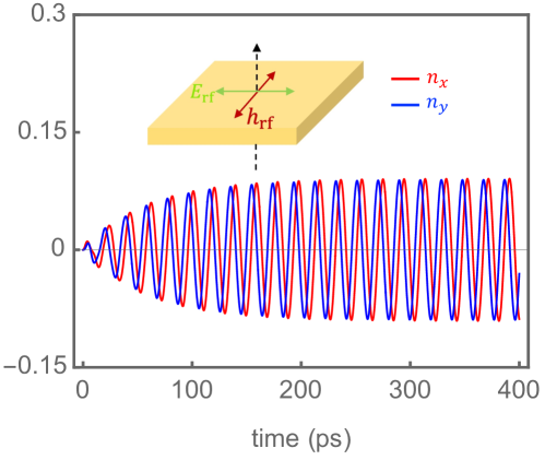
Figure S3: Time evolution of the Néel order $\bm{n}$ with the onset of AFM resonance (frequency: $f_{r}=51.9\ \mathrm{GHz}$) for an normally incident electromagnetic wave (inset). Parameters: $H_{J}=35$ T, $H_{\parallel}=0.16$ T, $H_{0}=1.5$ T, $\alpha=0.005$, $E_{x}=0.5\mathrm{V/\mu m}$, and $\Gamma=20$ meV

Next, we obtain the time evolution of the Néel vector $\bm{n}(t)$ by solving the LLG equations (4). Figure 5(a) and (b) plot the transverse components $n_{x}(t)$ and $n_{y}(t)$ for the two distinct cases under the resonance condition of the low-frequency mode: $f=\gamma\sqrt{\mathcal{H}_{\parallel}(\mathcal{H}_{\parallel}+2\mathcal{H}_{J})}-\gamma H_{0}$ [39], where $H_{0}=1.5$ T is applied along the $+z$ direction, yielding the low-frequency mode left-handed as illustrated by the inset of Fig. 5(d). With our chosen parameters, this $H_{0}$ field is well below the spin-flop threshold while separating the left-handed and right-handed modes by $84$ GHz. We emphasize that the vertical axis in Fig. 5(b) has a scale $15$ times larger than that in Fig. 5(a), and the amplitude of AFM resonance is about $20$ times larger in in Fig. 5(b) where the magnetic dynamics is activated by the $\bm{E}_{\rm rf}$ field (through the NSOT). To further confirm this point, we plot in Fig. S3 the case of a vertically incident microwave (along $z$) where both $\bm{h}_{\rm rf}$ and $\bm{E}_{\rm rf}$ can drive the magnetic dynamics. The result is hardly distinguishable from Fig. 5(b), indicating that the NSOT overwhelms the Zeeman coupling in driving the AFM resonance.

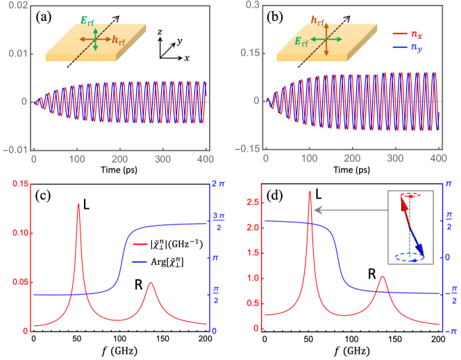
Figure 5: Time evolution of the Néel order $\bm{n}(t)$ at the resonance of the left-handed mode (with $f=51.9\ \mathrm{GHz}$ set by a bias field $H_{0}=1.5$ T) for (a) $\bm{h}_{\rm rf}$-driven configuration, and (b) $\bm{E}_{\rm rf}$-driven configuration. (c) and (d) are the corresponding amplitude (red, left axis) and phase (blue, right axis) of the dynamical susceptibility $\tilde{\chi}_{\perp}^{n}$ as a function of driving frequency $f$, where the low-frequency mode is left-handed (inset). Parameters: $H_{J}=35$ T, $H_{\parallel}=0.16$ T, $\alpha_{0}=0.005$, and $E_{\rm rf}=0.5\rm V/\mu m$ (corresponding to $h_{\rm rf}=16.5$ Gs).

Were not the NSOT generation, the electric field $\bm{E}_{\rm rf}$ is not even able to drive the spin dynamics, let alone entailing an enhanced resonance amplitude. To quantify the resonance absorption of the microwave, we linearlize the LLG equations (4) using the vectorial phasor representation: $\bm{m}^{A(B)}=\mathrm{Re}[\tilde{\bm{m}}^{A(B)}e^{\mathrm{i}\omega t}]$ and $\bm{h}_{D}^{A(B)}=\mathrm{Re}[\tilde{\bm{h}}_{D}^{A(B)}e^{\mathrm{i}\omega t}]$, with either $\tilde{\bm{h}}_{D}^{A}=\tilde{\bm{h}}_{D}^{B}=\tilde{h}_{\rm rf}\hat{\bm{x}}$ or $\tilde{\bm{h}}_{D}^{A}=-\tilde{\bm{h}}_{D}^{B}=\tilde{h}_{\rm NS}\hat{\bm{x}}$ depending on which component acts as the driving field. Since we have fixed the driving field to be polarized along $x$, the dynamical susceptibility of the Néel vector reduces to a vector $\tilde{\bm{\chi}}_{\perp}^{n}(\omega)=\{\tilde{\chi}^{n}_{x}(\omega),\ \tilde{\chi}^{n}_{y}(\omega)\}$ defined by

$$\tilde{n}_{x(y)}=\tilde{\chi}^{n}_{x(y)}(\omega)\gamma\tilde{h}_{D},$$ (5)

where $\tilde{h}_{D}=\tilde{h}_{\rm rf}$ for the geometry in Fig. 5(a), whereas $\tilde{h}_{D}=\tilde{h}_{\rm NS}$ for the geometry in Fig. 5(b). For simplicity, we set the initial phase of $\tilde{h}_{D}$ zero, so the phase difference between $\tilde{\bm{n}}$ and $\tilde{\bm{h}}_{D}$ is embedded in the phase of $\tilde{\bm{\chi}}_{\perp}^{n}(\omega)$. We numerically plot the amplitude $|\tilde{\bm{\chi}}^{n}_{\perp}|\equiv\sqrt{|\tilde{\chi}^{n}_{x}|^{2}+|\tilde{\chi}^{n}_{y}|^{2}}$ and the phase $\mathrm{Arg}[\tilde{\bm{\chi}}^{n}_{\perp}]\equiv\mathrm{Arg}[\tilde{\chi}^{n}_{x}]-\mathrm{Arg}[\tilde{\chi}^{n}_{y}]$ (in different colors) as a function of the frequency for the $\bm{h}_{\rm rf}$-driven resonance and the $\bm{E}_{\rm rf}$-driven resonance in Figs. 5 (c) and (d), respectively. Similar to the time-domain plots, here we intentionally adopt very different scales for the ordinates in Figs. 5 (c) and (d), which clearly shows that $|\tilde{\bm{\chi}}^{n}_{\perp}|$ (hence the microwave absorption) is about $20$ times larger when $\bm{E}_{\rm rf}$ activates the resonance (via the NSOT), as compared with the ordinary $\bm{h}_{\rm rf}$-driven mechanism (via direct Zeeman coupling). Basing on $\mathrm{Arg}[\tilde{\bm{\chi}}^{n}_{\perp}]$, we can further tell that the low-frequency mode indeed exhibits a left-handed precession of the Néel vector while the high-frequency mode is right-handed.

For ferromagnetic resonances [40], the power absorption rate at the resonance point is simply proportional to the amplitude of the dynamical susceptibility, given a fixed strength of the driving field. However, the case is subtly different when we turn to AFM resonances and look into the dynamical susceptibility of the Néel vector $\tilde{\bm{\chi}}^{n}_{\perp}(\omega)$. Even though we have considered a particular case where $h_{\rm rf}=h_{\rm NS}$, the actual power absorption rate under the $\bm{E}_{\rm rf}$-driven mechanism is not naïvely proportional to $|\tilde{\bm{\chi}}_{\perp}^{n}|$ ascribing to the staggered nature of the NSOT field ($\bm{h}_{\rm{NS}}^{A}=-\bm{h}_{\rm{NS}}^{B}$). In Method (Sec. B), we rigorously derive the time-averaged dissipation power for each mechanism, which allows us to quantify the ratio of the microwave power absorption rate under the two mechanisms as $\bar{P}_{E}/\bar{P}_{H}\approx 438.5$. The significantly enhanced microwave power absorption rate will greatly facilitate the detection of spin-torque excited AFM resonance.

To intuitively understand the pronounced difference in microwave absorption between the two mechanisms, we resort to the symmetry of NSOT. In contrast to the uniform Zeeman field $\bm{h}_{\rm rf}$ tending to kick $\bm{m}^{A}$ and $\bm{m}^{B}$ towards opposite directions, the NSOT field is itself opposite on the two sublattices, $\bm{h}_{\rm{NS}}^{A}=-\bm{h}_{\rm{NS}}^{B}$ [see Fig. 4 (d)], which drives the two magnetic moments towards the same direction, thus amplifying their non-collinearity. Consequently, the strong exchange interaction between $\bm{m}^{A}$ and $\bm{m}^{B}$ is leveraged to enhance the efficiency of magnetic dynamics, resulting in a much stronger absorption of the microwave.

VI Conclusion

In summary, we have studied the exotic topological phases, and the spin-torque generations in these phases, based on a G-type AFM material with a honeycomb lattice in the presence of the intrinsic SOC, the Rashba SOC and a staggered potential. We find that the highly non-trivial Néel-type SOT can not only be induced by an applied electrical field without producing Joule heating but also be utilized to drive the AFM resonance at a remarkably high efficiency which, even under a conservative estimate, is more than one order of magnitude larger than the traditional AFM resonance relying on the Zeeman coupling. Our significant findings opened a new exciting chapter of insulator-based spintronics.

Methods

VI.1 Chern number and spin Chern number

The topological Chern number is calculated by the Kubo formula [41, 42]:

$$C=-2\hbar^{2}\sum_{\epsilon_{n}<\epsilon_{f}<\epsilon_{m}}\mathrm{Im}\int_{\rm BZ}\frac{dk^{2}}{2\pi}\frac{\bra{n}\hat{v}_{x}\ket{m}\bra{m}\hat{v}_{y}\ket{n}}{(\epsilon_{n}-\epsilon_{m})^{2}},$$ (6)

where $\hbar$ is the reduced Planck constant, $\hat{v}_{i}=\partial\hat{H}/\hbar\partial k_{i}$ is the velocity operator and $\ket{n}$ is eigenstate corresponding to $\epsilon_{n}$. Similarly, the spin Chern number $C_{s}=(C_{\uparrow}-C_{\downarrow})/2$ is [21, 22]:

$$C_{s}=-2\hbar\sum_{\epsilon_{n}<\epsilon_{f}<\epsilon_{m}}\mathrm{Im}\int_{\mathrm{BZ}}\frac{dk^{2}}{2\pi}\frac{\bra{n}\hat{J}^{s}_{x}\ket{m}\bra{m}\hat{v}_{y}\ket{n}}{(\epsilon_{n}-\epsilon_{m})^{2}},$$ (7)

where $\hat{J}_{x}^{s}=\hbar(s_{z}\hat{v}_{x}+\hat{v}_{x}s_{z})/4$ is the spin-current operator along $x$ with the spin polarization along $z$. The numerical calculation of the band structure and the spatial distribution of the scattering states are performed by Kwant [43].

VI.2 Microwave power absorption

When a steady-state dynamics is established, the density of microwave power absorption $P_{H}$ should be fully balanced by the magnetic dissipation power density $P_{m}=-m_{s}\bm{h}_{D}\cdot(\dot{\bm{m}}^{A}+\dot{\bm{m}}^{B})/V_{\rm uc}$ upon time averaging, where $V_{\rm uc}$ is the unit cell volume (area).

Case I. When the driving field $\bm{h}_{D}$ is the magnetic component $\bm{h}_{\rm rf}$ of the electromagnetic wave, which is polarized along $x$ [Fig. 5(a)], our convention assumes $h_{\rm rf}(t)={\rm Re}[\tilde{h}_{\rm rf}e^{\mathrm{i}\omega t}]=H_{x}\cos(\omega t)$, and $\bm{m}^{A(B)}(t)={\rm Re}[\tilde{\bm{m}}^{A(B)}e^{\mathrm{i}\omega t}]$ where $\bm{\tilde{m}}^{A(B)}=\{\tilde{m}^{A(B)}_{x}e^{\mathrm{i}\omega t},\ \tilde{m}^{A(B)}_{y}e^{\mathrm{i}\omega t},\ 1\}$. By linearizing the LLG equations around the equilibrium position of each magnetic sublattice, we obtain $\tilde{m}^{A(B)}_{x}=\tilde{\chi}^{A(B)}_{x}(\omega)\gamma\tilde{h}_{\rm rf}$ and $\tilde{m}^{A(B)}_{y}=\tilde{\chi}^{A(B)}_{y}(\omega)\gamma\tilde{h}_{\rm rf}$. Therefore, the instantaneous power density $P_{m}(t)$ is

$$P_{m}(t) =-\frac{\gamma m_{s}}{V_{\rm uc}}{\rm Re}[(\tilde{\chi}^{A}_{x}+\tilde{\chi}^{B}_{x})\mathrm{i}\omega e^{\mathrm{i}\omega t}]\cos(\omega t)H_{x}^{2}$$

$$=-\frac{\gamma m_{s}}{V_{\rm uc}}|\tilde{\chi}^{+}_{x}|{\rm Re}[\mathrm{i}\omega e^{\mathrm{i}(\omega t+\phi^{+})}]\cos(\omega t)H_{x}^{2}$$

$$=\frac{\gamma m_{s}}{V_{\rm uc}}|\tilde{\chi}^{+}_{x}|\omega\sin(\omega t+\phi^{+})\cos(\omega t)H_{x}^{2},$$ (8)

where we have defined $\tilde{\chi}^{+}_{x}\equiv\tilde{\chi}^{A}_{x}+\tilde{\chi}^{B}_{x}=|\tilde{\chi}^{+}_{x}|e^{\mathrm{i}\phi^{+}}$. Some straightforward algebra shows that

$$\tilde{\chi}^{+}_{x}(\omega)=(\mathrm{i}\omega\alpha-\omega_{A})\left[\frac{1}{D^{+}(\omega)}+\frac{1}{D^{-}(\omega)}\right],$$ (9)

where $D^{\pm}(\omega)\equiv(\omega\pm\omega_{0})^{2}-\omega_{A}(\omega_{A}+2\omega_{J})+2\mathrm{i}\omega(\omega_{A}+\omega_{J})\alpha+(\omega\alpha)^{2}$ with $\omega_{A}=\gamma\mathcal{H}_{\parallel}$, $\omega_{0}=\gamma\mathcal{H}_{0}$, and $\omega_{J}=\gamma\mathcal{H}_{J}$. By averaging over time, we find

$$\overline{P}_{H}=\overline{P}_{m}=\frac{m_{s}\gamma H_{x}^{2}}{2V_{\rm uc}}\omega|\tilde{\chi}^{+}_{x}(\omega)|\sin[\phi^{+}(\omega)],$$ (10)

which is maximized for $\phi^{+}=\pi/2$ (at the resonance peak). Phenomenologically, $\phi^{+}=\pi/2$ indicates that $\bm{h}_{\rm rf}(t)\cdot\bm{m}^{A(B)}(t)=0$ so that $\bm{h}_{\rm rf}(t)\parallel\dot{\bm{m}}^{A(B)}(t)$.

Case II. When the driving field $\bm{h}_{D}$ is the NSOT field $\bm{h}_{\rm NS}$ generated by the electric component $\bm{E}_{\rm rf}$ of the electromagnetic wave, we have shown in Ref [13] in a generic context that $P_{m}=-m_{s}\alpha[(\dot{\bm{m}}^{A})^{2}+(\dot{\bm{m}}^{B})^{2}]/\gamma V_{\rm uc}$, which, in a steady-state dynamics, balances the electrical power $P_{E}=\bm{J}^{\rm ad}\cdot\bm{E}$ with $\bm{J}^{\rm ad}$ being the adiabatic current density pumped by the magnetic dynamics, while the conduction current (i.e., Ohm’s current) vanishes identically inside the insulator. For an $\bm{E}_{\rm rf}=E_{x}\cos(\omega t)\hat{\bm{x}}$ [Fig. 5(b)], the time-averaged electrical power density is

$$\overline{P}_{E}=\overline{P}_{m}=\frac{1}{2}E_{x}^{2}{\rm Re}[\tilde{\sigma}_{xx}(\omega)],$$ (11)

where $\tilde{\sigma}_{xx}(\omega)$ is the effective longitudinal conductivity, $\tilde{\sigma}_{xx}=\tilde{J}_{x}^{\rm ad}/\tilde{E}_{x}$. Microscopically, $\tilde{\sigma}_{xx}(\omega)$ is determined by the Berry curvature in the mixed momentum and magnetization space [12]:

$$\tilde{\sigma}_{xx} =\mathrm{i}\omega\frac{\gamma e^{2}}{m_{s}V_{\rm uc}}\left\langle\Omega_{xx}^{km^{A}}\right\rangle^{2}\left[\tilde{\eta}^{A}_{x}(\omega)-\tilde{\eta}^{B}_{x}(\omega)\right],$$ (12)

where the Berry curvature $\Omega^{km}$ is the same as that in Eq. (3) and we have invoked the relation $\langle\Omega^{km^{A}}_{xx}\rangle=-\langle\Omega^{km^{B}}_{xx}\rangle$ for $\lambda_{v}=0$ and $\Gamma=0$. In this case, the dynamical susceptibility relates the NSOT field to the magnetic moments as $\tilde{m}^{A(B)}_{x}=\tilde{\eta}^{A(B)}_{x}(\omega)\gamma\tilde{h}_{\rm NS}^{A(B)}$ where

$$\tilde{h}_{\rm NS}^{A}=-\tilde{h}_{\rm NS}^{B}=-\frac{2\lambda_{ex}}{\hbar m_{s}}\delta\tilde{S}^{A}_{x}=-\frac{e}{m_{s}}\langle\Omega^{km^{A}}_{xx}\rangle\tilde{E}_{x}$$ (13)

is polarized along $x$ because $\bm{E}_{\rm rf}$ is polarized along $x$. Here we used a different notation $\tilde{\eta}$ to represent the dynamical susceptibility just to avoid confusion about Case II with Case I. We then arrive at the final expression for the power absorption rate

$$\overline{P}_{E}= \frac{\gamma e^{2}\omega E_{x}^{2}}{2m_{s}V_{\rm uc}}\left\langle\Omega^{km^{A}}_{xx}\right\rangle^{2}{\rm Re}[\mathrm{i}(\tilde{\eta}^{A}_{x}-\tilde{\eta}^{B}_{x})]$$

$$= -\frac{\gamma e^{2}}{2m_{s}V_{\rm uc}}\left\langle\Omega^{km^{A}}_{xx}\right\rangle^{2}\omega|\tilde{\eta}^{-}_{x}(\omega)|\sin[\varphi^{-}(\omega)]E_{x}^{2},$$ (14)

where we have defined $\tilde{\eta}^{-}_{x}\equiv\tilde{\eta}^{A}_{x}-\tilde{\eta}^{B}_{x}=|\tilde{\eta}^{-}_{x}|e^{\mathrm{i}\varphi^{-}}$, for which we find

$$\tilde{\eta}^{-}_{x}(\omega)=(\mathrm{i}\omega\alpha-\omega_{A}-2\omega_{J})\left[\frac{1}{D^{+}(\omega)}+\frac{1}{D^{-}(\omega)}\right].$$ (15)

Comparing with $\tilde{\chi}^{+}_{x}$, an extra term $2\omega_{J}$ appears in the front factor, which overwhelms $\mathrm{i}\omega\alpha-\omega_{A}$. Similar to the previous case, $\overline{P}_{E}$ is maximized for $\varphi^{-}=\pi/2$ (at the resonance peak).

We can now compare the ratio of power absorption for the two cases:

$$\frac{\overline{P}_{E}}{\overline{P}_{H}}=\left[\frac{e\left\langle\Omega^{km^{A}}_{xx}\right\rangle}{m_{s}}\right]^{2}\left(\frac{E_{x}}{H_{x}}\right)^{2}\frac{|\tilde{\eta}_{x}^{-}|\sin\phi^{-}}{|\tilde{\chi}_{x}^{+}|\sin\phi^{+}},$$ (16)

which, when taking into account that $|\tilde{h}_{\rm rf}|=H_{x}$ and the NSOT field $|\tilde{h}_{\rm NS}|=|eE_{x}\langle\Omega^{km^{A}}_{xx}\rangle/m_{s}|$, becomes

$$\frac{\overline{P}_{E}}{\overline{P}_{H}}=\frac{{h}_{\rm NS}^{2}|\tilde{\eta}_{x}^{-}|\sin\varphi^{-}}{{h}_{\rm rf}^{2}|\tilde{\chi}_{x}^{+}|\sin\phi^{+}}.$$ (17)

As we set ${h}_{\rm NS}={h}_{\rm rf}$ in the main text for comparing the two cases, this ratio can be evaluated at the resonance point where $\omega=\sqrt{\omega_{A}(\omega_{A}+2\omega_{E})}-\omega_{0}$ and $\varphi^{-}(\omega_{r})\approx\phi^{+}(\omega_{r})\approx\pi/2$:

$$\frac{\overline{P}_{E}}{\overline{P}_{H}}=\left\|\frac{\mathrm{i}\omega_{r}\alpha-\omega_{A}-2\omega_{J}}{\mathrm{i}\omega_{r}\alpha-\omega_{A}}\right\|\approx 438.5$$ (18)

Reference

Supplemental Materials

References

- Otrokov et al. [2019a] M. M. Otrokov, I. I. Klimovskikh, H. Bentmann, D. Estyunin, A. Zeugner, Z. S. Aliev, S. Gaß, A. Wolter, A. Koroleva, A. M. Shikin, et al., Prediction and observation of an antiferromagnetic topological insulator, Nature 576, 416 (2019a).
- Chen et al. [2019a] B. Chen, F. Fei, D. Zhang, B. Zhang, W. Liu, S. Zhang, P. Wang, B. Wei, Y. Zhang, Z. Zuo, et al., Intrinsic magnetic topological insulator phases in the Sb doped bulks and thin flakes, Nature communications 10, 4469 (2019a).
- Li et al. [2019] J. Li, Y. Li, S. Du, Z. Wang, B.-L. Gu, S.-C. Zhang, K. He, W. Duan, and Y. Xu, Intrinsic magnetic topological insulators in van der waals layered mnbi2te4-family materials, Science Advances 5, eaaw5685 (2019).
- Zhang et al. [2019] D. Zhang, M. Shi, T. Zhu, D. Xing, H. Zhang, and J. Wang, Topological Axion States in the Magnetic Insulator with the Quantized Magnetoelectric Effect, Phys. Rev. Lett. 122, 206401 (2019).
- Gong et al. [2019] Y. Gong, J. Guo, J. Li, K. Zhu, M. Liao, X. Liu, Q. Zhang, L. Gu, L. Tang, X. Feng, D. Zhang, W. Li, C. Song, L. Wang, P. Yu, X. Chen, Y. Wang, H. Yao, W. Duan, Y. Xu, S.-C. Zhang, X. Ma, Q.-K. Xue, and K. He, Experimental realization of an intrinsic magnetic topological insulator, Chinese Physics Letters 36, 076801 (2019).
- Deng et al. [2020] Y. Deng, Y. Yu, M. Shi, Z. Guo, Z. Xu, J. Wang, X. Chen, and Y. Zhang, Quantum anomalous Hall effect in intrinsic magnetic topological insulator , Science 367, 10.1126/science.aax8156 (2020).
- Liu et al. [2020] C. Liu, Y. Wang, H. Li, Y. Wu, Y. Li, J. Li, K. He, Y. Xu, J. Zhang, and Y. Wang, Robust axion insulator and chern insulator phases in a two-dimensional antiferromagnetic topological insulator, Nature Materials 19, 522 (2020).
- Ovchinnikov et al. [2021] D. Ovchinnikov, X. Huang, Z. Lin, Z. Fei, J. Cai, T. Song, M. He, Q. Jiang, C. Wang, H. Li, et al., Intertwined topological and magnetic orders in atomically thin Chern insulator , Nano letters 21, 2544 (2021).
- Yang et al. [2021] S. Yang, X. Xu, Y. Zhu, R. Niu, C. Xu, Y. Peng, X. Cheng, X. Jia, Y. Huang, X. Xu, J. Lu, and Y. Ye, Odd-Even Layer-Number Effect and Layer-Dependent Magnetic Phase Diagrams in , Phys. Rev. X 11, 011003 (2021).
- Zhao et al. [2021] Y.-F. Zhao, L.-J. Zhou, F. Wang, G. Wang, T. Song, D. Ovchinnikov, H. Yi, R. Mei, K. Wang, M. H. Chan, et al., Even–odd layer-dependent anomalous Hall effect in topological magnet thin films, Nano letters 21, 7691 (2021).
- Otrokov et al. [2019b] M. M. Otrokov, I. P. Rusinov, M. Blanco-Rey, M. Hoffmann, A. Y. Vyazovskaya, S. V. Eremeev, A. Ernst, P. M. Echenique, A. Arnau, and E. V. Chulkov, Unique Thickness-Dependent Properties of the van der Waals Interlayer Antiferromagnet Films, Phys. Rev. Lett. 122, 107202 (2019b).
- Tang and Cheng [2024] J. Tang and R. Cheng, Lossless spin-orbit torque in antiferromagnetic topological insulator , Phys. Rev. Lett. 132, 136701 (2024).
- Tang and Cheng [2022] J.-Y. Tang and R. Cheng, Voltage-driven exchange resonance achieving mechanical efficiency, Phys. Rev. B 106, 054418 (2022).
- Feng et al. [2024] X. Feng, J. Cao, Z.-F. Zhang, L. K. Ang, S. Lai, H. Jiang, C. Xiao, and S. A. Yang, Intrinsic dynamic generation of spin polarization by time-varying electric field, arXiv preprint arXiv:2409.09669 10.48550/arXiv.2409.09669 (2024).
- Kane and Mele [2005a] C. L. Kane and E. J. Mele, topological order and the quantum spin hall effect, Phys. Rev. Lett. 95, 146802 (2005a).
- Kane and Mele [2005b] C. L. Kane and E. J. Mele, Quantum spin hall effect in graphene, Phys. Rev. Lett. 95, 226801 (2005b).
- Chang et al. [2023] C.-Z. Chang, C.-X. Liu, and A. H. MacDonald, Colloquium: Quantum anomalous hall effect, Rev. Mod. Phys. 95, 011002 (2023).
- Liu et al. [2016] C.-X. Liu, S.-C. Zhang, and X.-L. Qi, The quantum anomalous hall effect: Theory and experiment, Annual Review of Condensed Matter Physics 7, 301 (2016).
- Maciejko et al. [2011] J. Maciejko, T. L. Hughes, and S.-C. Zhang, The quantum spin hall effect, Annu. Rev. Condens. Matter Phys. 2, 31 (2011).
- König et al. [2008] M. König, H. Buhmann, L. W. Molenkamp, T. Hughes, C.-X. Liu, X.-L. Qi, and S.-C. Zhang, The quantum spin hall effect: theory and experiment, Journal of the Physical Society of Japan 77, 031007 (2008).
- Sheng et al. [2006] D. N. Sheng, Z. Y. Weng, L. Sheng, and F. D. M. Haldane, Quantum spin-hall effect and topologically invariant chern numbers, Phys. Rev. Lett. 97, 036808 (2006).
- Sheng et al. [2005] L. Sheng, D. N. Sheng, C. S. Ting, and F. D. M. Haldane, Nondissipative spin hall effect via quantized edge transport, Phys. Rev. Lett. 95, 136602 (2005).
- Guo et al. [2023] P.-J. Guo, Z.-X. Liu, and Z.-Y. Lu, Quantum anomalous hall effect in collinear antiferromagnetism, npj Computational Materials 9, 70 (2023).
- Lei et al. [2022] C. Lei, T. V. Trevisan, O. Heinonen, R. J. McQueeney, and A. H. MacDonald, Quantum anomalous hall effect in perfectly compensated collinear antiferromagnetic thin films, Phys. Rev. B 106, 195433 (2022).
- Šmejkal et al. [2022] L. Šmejkal, A. H. MacDonald, J. Sinova, S. Nakatsuji, and T. Jungwirth, Anomalous hall antiferromagnets, Nature Reviews Materials 7, 482 (2022).
- Edelstein [1990] V. M. Edelstein, Spin polarization of conduction electrons induced by electric current in two-dimensional asymmetric electron systems, Solid State Communications 73, 233 (1990).
- Shao et al. [2016] Q. Shao, G. Yu, Y.-W. Lan, Y. Shi, M.-Y. Li, C. Zheng, X. Zhu, L.-J. Li, P. K. Amiri, and K. L. Wang, Strong rashba-edelstein effect-induced spin–orbit torques in monolayer transition metal dichalcogenide/ferromagnet bilayers, Nano letters 16, 7514 (2016).
- Mellnik et al. [2014] A. Mellnik, J. Lee, A. Richardella, J. Grab, P. Mintun, M. H. Fischer, A. Vaezi, A. Manchon, E.-A. Kim, N. Samarth, et al., Spin-transfer torque generated by a topological insulator, Nature 511, 449 (2014).
- Li et al. [2020] X. Li, H. Chen, and Q. Niu, Out-of-plane carrier spin in transition-metal dichalcogenides under electric current, Proceedings of the National Academy of Sciences 117, 16749 (2020).
- Sokolewicz et al. [2019] R. Sokolewicz, S. Ghosh, D. Yudin, A. Manchon, and M. Titov, Spin-orbit torques in a rashba honeycomb antiferromagnet, Phys. Rev. B 100, 214403 (2019).
- Železný et al. [2014] J. Železný, H. Gao, K. Výborný, J. Zemen, J. Mašek, A. Manchon, J. Wunderlich, J. Sinova, and T. Jungwirth, Relativistic néel-order fields induced by electrical current in antiferromagnets, Phys. Rev. Lett. 113, 157201 (2014).
- Bodnar et al. [2018] S. Y. Bodnar, L. Šmejkal, I. Turek, T. Jungwirth, O. Gomonay, J. Sinova, A. Sapozhnik, H.-J. Elmers, M. Kläui, and M. Jourdan, Writing and reading antiferromagnetic by Néel spin-orbit torques and large anisotropic magnetoresistance, Nature communications 9, 348 (2018).
- Chen et al. [2019b] X. Chen, X. Zhou, R. Cheng, C. Song, J. Zhang, Y. Wu, Y. Ba, H. Li, Y. Sun, Y. You, et al., Electric field control of néel spin–orbit torque in an antiferromagnet, Nature materials 18, 931 (2019b).
- Behovits et al. [2023] Y. Behovits, A. L. Chekhov, S. Y. Bodnar, O. Gueckstock, S. Reimers, Y. Lytvynenko, Y. Skourski, M. Wolf, T. S. Seifert, O. Gomonay, et al., Terahertz Néel spin-orbit torques drive nonlinear magnon dynamics in antiferromagnetic , Nature Communications 14, 6038 (2023).
- Bodnar et al. [2019] S. Y. Bodnar, M. Filianina, S. Bommanaboyena, T. Forrest, F. Maccherozzi, A. Sapozhnik, Y. Skourski, M. Kläui, and M. Jourdan, Imaging of current induced Néel vector switching in antiferromagnetic , Physical Review B 99, 140409 (2019).
- Wildes et al. [1998] A. Wildes, B. Roessli, B. Lebech, and K. Godfrey, Spin waves and the critical behaviour of the magnetization in , Journal of Physics: Condensed Matter 10, 6417 (1998).
- Long et al. [2020] G. Long, H. Henck, M. Gibertini, D. Dumcenco, Z. Wang, T. Taniguchi, K. Watanabe, E. Giannini, and A. F. Morpurgo, Persistence of magnetism in atomically thin crystals, Nano letters 20, 2452 (2020).
- Kim et al. [2019] K. Kim, S. Y. Lim, J. Kim, J.-U. Lee, S. Lee, P. Kim, K. Park, S. Son, C.-H. Park, J.-G. Park, et al., Antiferromagnetic ordering in van der Waals 2D magnetic material probed by Raman spectroscopy, 2D Materials 6, 041001 (2019).
- Keffer and Kittel [1952] F. Keffer and C. Kittel, Theory of antiferromagnetic resonance, Phys. Rev. 85, 329 (1952).
- Kittel [1948] C. Kittel, On the theory of ferromagnetic resonance absorption, Phys. Rev. 73, 155 (1948).
- Thouless et al. [1982] D. J. Thouless, M. Kohmoto, M. P. Nightingale, and M. den Nijs, Quantized hall conductance in a two-dimensional periodic potential, Phys. Rev. Lett. 49, 405 (1982).
- Xiao et al. [2010] D. Xiao, M.-C. Chang, and Q. Niu, Berry phase effects on electronic properties, Rev. Mod. Phys. 82, 1959 (2010).
- Groth et al. [2014] C. W. Groth, M. Wimmer, A. R. Akhmerov, and X. Waintal, Kwant: a software package for quantum transport, New Journal of Physics 16, 063065 (2014).