Reliable and Compact Graph Fine-tuning via Graph Sparse Prompting

Abstract

Recently, graph prompt learning has garnered increasing attention in adapting pre-trained GNN models for downstream graph learning tasks. However, existing works generally conduct prompting over all graph elements (e.g., nodes, edges, node attributes, etc.), which is suboptimal and obviously redundant. To address this issue, we propose exploiting sparse representation theory for graph prompting and present Graph Sparse Prompting (GSP). GSP aims to adaptively and sparsely select the optimal elements (e.g., certain node attributes) to achieve compact prompting for downstream tasks. Specifically, we propose two kinds of GSP models, termed Graph Sparse Feature Prompting (GSFP) and Graph Sparse multi-Feature Prompting (GSmFP). Both GSFP and GSmFP provide a general scheme for tuning any specific pre-trained GNNs that can achieve attribute selection and compact prompt learning simultaneously. A simple yet effective algorithm has been designed for solving GSFP and GSmFP models. Experiments on 16 widely-used benchmark datasets validate the effectiveness and advantages of the proposed GSFPs.

I Introduction

Graph Neural Networks (GNNs) have become a powerful tool for analyzing graph-structured data, with practical applications in many fields such as social network analysis [1], drug discovery [2], fraud detection [3] and traffic prediction [4]. However, GNNs often rely on supervised learning, which demands large amounts of task-specific labeled data. Acquiring such labeled data is time-consuming and expensive, limiting the practical application of GNNs in many real-world scenarios. To reduce dependence on labeled data, researchers have explored ‘pre-training + fine-tuning’ strategy [5]. This strategy first learns useful representations from large-scale unlabeled data to enhance the generalization ability of GNNs and then fine-tunes the pre-trained model on the downstream tasks with a small amount of labeled data. However, due to the discrepancy between the pre-training and downstream stages in different graph domains, direct fine-tuning may result in suboptimal performance or even lead to negative transfer [6]. Also, full fine-tuning the pre-trained model is usually time-consuming and computationally expensive.

To overcome these issues, graph prompt learning techniques have been developed for fine-tuning pre-trained GNN models. By reformulating the downstream data/task to better align with the pre-training phase, these techniques can reduce the gap between the pre-training and downstream stages [7]. Overall, existing graph prompt learning methods can be mainly categorized into two types, i.e., task aligning and graph data prompting. For task aligning prompting, some works focus on constructing prompt templates to unify the pre-training objective and downstream task. For example, GPPT [8] converts the downstream node classification task into the pre-trained link prediction task. GraphPrompt [9] transforms both link prediction in pre-training and the downstream node/graph classification into general subgraph similarity computation. In work [10], it translates both node-level and edge-level downstream tasks into unified graph-level tasks. For graph data prompting, some works aim to conduct prompting directly on the input graph nodes or edges. For graph edge prompting, AAGOD[11] proposes edge-level prompt by adjusting edge weights in the adjacency matrix with a learnable amplifier. PSP[12] adds weighted connection edges between class prototype nodes and original nodes in the input graph as structure prompt. For graph node prompting, GraphPrompt [9] multiplies the hidden node features with a learnable prompt vector to assist the readout operation. All-in-One [10] designs the prompt as a graph composed of a set of prompt nodes and inserts it into the input graph. GPF [13] and GPF-plus [13] directly add prompt vectors to the input node features. Other graph prompt designs [14, 15, 16] can generally be seen as special cases or natural extensions of GPF and All-in-One. Some works [13, 17] have theoretically proven the effectiveness of these prompt methods. In this paper, we mainly focus on graph node prompt learning.

After reviewing the above existing graph prompting methods, we observe that they generally conduct prompting over all graph elements, such as nodes, edges or node attributes. For example, VNT [16] sends the prompt nodes and the original node set into the Graph Transformer together to achieve prompting on all nodes. GPF [13] conducts prompting on all node attributes. However, in many downstream tasks, graphs are usually complex, such as large scale, dense edges or high attribute dimension. Therefore, two natural questions emerge: Is it necessary to conduct prompting on all graph elements? What are the most desirable elements needing to be prompted?

To address these questions, for the first time, we propose a new prompt learning problem for graph fine-tuning, termed Graph Sparse Prompting (GSP). Generally speaking, our GSP problem is defined as adaptively and sparsely selecting the optimal elements to achieve compact prompting for downstream tasks. In this paper, we mainly focus on node attribute prompting scheme, i.e., Graph Prompt Feature (GPF) [13], which aims to conduct prompting on graph node attributes. In this case, our GSP problem is specifically defined as sparsely selecting some reliable node attributes for prompting. We show that this goal can be well formulated by introducing some sparsity-inducing constraint/regularization into the objective of graph prompt optimization, as inspired by sparse representation theory [18, 19] in machine learning field. Specifically, we propose two kinds of graph sparse prompting over attributes, termed Graph Sparse Feature Prompting (GSFP) and Graph Sparse multi-Feature Prompting (GSmFP). Both GSFP and GSmFP provide a general framework for tuning any specific pre-trained GNNs, which can achieve attribute selection and compact prompt learning simultaneously without requiring any additional trainable parameters. A simple yet effective algorithm has been designed for solving GSFP and GSmFP problem.

Overall, the main contributions of this paper are summarized as follows,

• We introduce a new prompt problem, termed graph sparse prompting, for reliable and compact graph fine-tuning.

• We propose some sparsity-inducing regularizations into the graph prompt optimization and develop two kinds of graph prompts, i.e., Graph Sparse Feature Prompting (GSFP) and Graph Sparse multi-Feature Prompting (GSmFP) for graph fine-tuning.

• We derive a simple yet effective algorithm to optimize the proposed GSFP and GSmFP.

Experiments on 16 widely-used benchmark datasets validate the effectiveness and advantages of the proposed GSFP and GSmFP approaches.

II Related Works

II-A Graph Pre-training

By learning transferable representations from large-scale unlabeled data [5], pre-training can enhance the generalization ability of GNNs and reduce the need for large annotated datasets. DGI [20] maximizes the mutual information between local node features and global graph embedding. GraphMAE [21] applies a masked autoencoder to reconstruct masked node features for unsupervised representation learning. EdgePred [22, 8] predicts the existence of edges between nodes to capture local structural patterns. GraphCL [23] performs contrastive learning by maximizing the consistency between different augmented views of the same graph. SimGRACE [24] uses a GNN model along with its perturbed version as two encoders to generate two correlated representations for contrasting which can simplify the contrastive learning process. However, most graph pre-training methods follow the ‘pre-training + fine-tuning’ paradigm. Due to the gap between pre-training and fine-tuning stages, the fine-tuned model may perform suboptimally or even worse than training from scratch [25].

II-B Graph Prompt Learning

Graph prompt learning [7] has recently emerged as a novel paradigm inspired by prompt learning in natural language processing (NLP) and computer vision (CV). Unlike the traditional ‘pre-training + fine-tuning’ paradigm, graph prompt learning introduces prompts to guide the learning process while keeping the pre-trained model parameters frozen and only fine-tuning the prompts. There are two main types of approaches, i.e., task aligning prompting and graph data prompting.

Task Aligning Prompting. To address the gap between different graph learning tasks, some works aim to create unified task templates to align the pre-training and downstream tasks. For example, GPPT [8] uses link prediction as pre-training and uses prompt tokens to turn node classification into its pre-training task. GraphPrompt[9] constructs a graph similarity template to unify pre-training and downstream tasks. All-in-One [10] transforms both node-level and edge-level tasks into graph level-tasks. PRODIGY [26] uses a neighbor matching task for pre-training and employs prompt graphs to express downstream tasks as pre-training tasks. OFA [27] unifies different tasks into the same node binary classification.

Graph Data Prompting. In addition to task aligning prompting, some works facilitate the transfer of pre-trained knowledge by adding learnable prompts into the model’s input or hidden layer. For example, VNT [16] adds learnable prompt nodes to the original node set and then feeds them into the pre-trained Graph Transformer for information aggregation. All-in-One[10] designs prompt as graph and considers the connection between input graph and prompt graph. GPF [13] adds the same learnable prompt vector to each node feature during the input phase. GPF-plus [13] further assigns different prompts to each node feature via cross-attention module. GraphPrompt[9] multiplies the output data of model’s hidden layer with a learnable prompt vector to assist the readout operation. HetGPT[28] introduces a small number of trainable parameters into the node features of the heterogeneous graph to generate prompted node features. HGPrompt [29] introduces feature prompt and heterogeneity prompt to modify the node features in the readout operation and auxiliary aggregation operation. MDGPT [30] utilizes dual prompts to modify the downstream input features, facilitating the transfer of pre-trained knowledge to the target domain.

III Preliminary

In this section, we briefly introduce two kinds of graph prompt learning methods, i.e., Graph Prompt Feature (GPF) [13] and Graph Prompt Feature-Plus (GPF-plus) [13]. Given a pre-trained GNN model $f_{\Phi}$ with parameters $\Phi$ and an input graph $\mathcal{G}(\mathbf{X},\mathbf{A})$, the data prompt-based fine-tuning process can be formulated as follows,

$$\{\theta^{*},\tilde{\mathcal{G}}^{*}\}=\text{argmin}\,\,\,\mathcal{L}^{down}\big{(}f_{\Phi}(\tilde{\mathcal{G}}(\tilde{{\textbf{X}}},\tilde{\textbf{A}})),\theta\big{)}$$ (1)

where $\tilde{\mathcal{G}}(\tilde{{\textbf{X}}},\tilde{{\textbf{A}}})$ denotes the prompted graph generated by employing some prompting functions to adjust node features or edge weights for the downstream task, and $\theta$ denotes the learnable parameters in the downstream task, such as the task-specific classifier head.

One important way to obtain the prompted graph is to adjust graph node features by adding some learnable prompt vectors to the node features/attributes, which is called Graph Prompt Feature (GPF) [13]. To be specific, given an input graph $\mathcal{G}(\textbf{X},\textbf{A})$, where $\textbf{X}\in\mathbb{R}^{n\times d}$ denotes the node feature matrix and $\textbf{A}\in\mathbb{R}^{n\times n}$ represents the adjacency matrix, GPF generates a prompted graph $\tilde{\mathcal{G}}(\tilde{\textbf{X}},\textbf{A})$ by adding a shared learnable prompt vector $\textbf{p}\in\mathbb{R}^{d}$ to each node features as,

$$\tilde{\textbf{X}}=\textbf{X}+\textbf{1}\textbf{p}^{T}$$ (2)

where 1 is a column vector of ones with dimension $n$. Hence, the above formulation Eq.(1) for GPF can be specified as,

$$\min_{\theta,\textbf{p}}\,\,\mathcal{L}^{down}\big{(}f_{\Phi}(\tilde{\mathcal{G}}(\tilde{\textbf{X}},\textbf{A})),\theta\big{)}$$ (3)

$$s.t.\,\,\tilde{\textbf{X}}=\textbf{X}+\textbf{1}\textbf{p}^{T}$$

Beyond a single prompt vector, GPF-plus [13] further assigns a prompt vector to each node by using $k$ independent prompt basis vectors $\textbf{P}=[\textbf{p}_{1},\textbf{p}_{2},\ldots,\textbf{p}_{k}]\in\mathbb{R}^{d\times k}$. It employs a cross-attention mechanism to assign these prompt vectors to all nodes as,

$$\tilde{\textbf{X}}=\textbf{X}+\textbf{S}\textbf{P}^{T},\,\textrm{where}\,\,\textbf{S}_{ij}=\frac{\exp(\textbf{b}_{j}^{T}\textbf{x}_{i})}{\sum_{l=1}^{k}\exp(\textbf{b}_{l}^{T}\textbf{x}_{i})}$$ (4)

where $\textbf{B}=[\textbf{b}_{1},\textbf{b}_{2},\ldots,\textbf{b}_{k}]\in\mathbb{R}^{d\times k}$ are $k$ learnable linear projections. When $k=1$, GPF-plus degenerates to a ‘weighted’ GPF. For convenience, in the following presentation, we include B in the learnable parameters $\theta$. Therefore, the above formulation Eq.(1) for GPF-plus can be specified as,

$$\min_{\theta,\textbf{P}}\,\,\mathcal{L}^{down}\big{(}f_{\Phi}(\tilde{\mathcal{G}}(\tilde{\textbf{X}},\textbf{A})),\theta\big{)}$$ (5)

$$s.t.\,\,\tilde{\textbf{X}}=\textbf{X}+\textbf{S}\textbf{P}^{T}$$

Note that, the optimal $\theta^{*}$ and $\textbf{P}^{*}$ can be learned by using the gradient descent algorithm.

IV Graph Sparse Feature Prompting

As shown in Eqs.(3,5), the above GPFs adopt the deterministic prompting mechanism on all node attributes (features). This ‘complete’ prompting mechanism is obviously redundant and suboptimal. To overcome these issues, one straightforward way is to select some reliable/meaningful attributes for prompting, allowing the model to focus on some most relevant features. This can be achieved by adding a $\ell_{0}$-norm sparse constraint on prompt vector p in Eq.(3) as,

$$\min_{\theta,\textbf{p}}\,\,\mathcal{L}^{down}\big{(}f_{\Phi}(\tilde{\mathcal{G}}(\tilde{\textbf{X}},\textbf{A})),\theta\big{)}$$ (6)

$$s.t.\,\,\tilde{\textbf{X}}=\textbf{X}+\textbf{1}\textbf{p}^{T},\|\textbf{p}\|_{0}\leq m$$

where $\|\textbf{p}\|_{0}$ denotes the number of non-zero elements in prompt vector p. This constraint encourages the learned p to be sparse, thereby naturally enabling the addition of prompt elements to be conducted only on some feature dimensions. In this paper, we call it as Graph Sparse Feature Prompting (GSFP). Since $\ell_{0}$-norm constraint is discrete and non-convex, it is difficult to optimize it directly. Similar to Lasso [31], we use $\ell_{1}$-norm regularization to approximate the above problem as follows,

$$\min_{\theta,\textbf{p}}\,\,\mathcal{L}^{down}\big{(}f_{\Phi}(\tilde{\mathcal{G}}(\tilde{\textbf{X}},\textbf{A})),\theta\big{)}+\lambda\|\textbf{p}\|_{1}$$ (7)

$$s.t.\,\,\tilde{\textbf{X}}=\textbf{X}+\textbf{1}\textbf{p}^{T}$$

where $\lambda>0$ is the penalty parameter and $\|\textbf{p}\|_{1}=\sum_{i}|\textbf{p}_{i}|$ denotes the $\ell_{1}$-norm function. Figure 1 shows the intuitive explanation of our GSFP model.

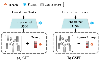
Figure 1: Comparing GPF and our method GSFP. GPF conducts prompting on every dimension of node features. In contrast, GSFP aims to conduct prompting on certain specific feature dimensions.

The above GSFP can also be extended to the multiple prompts learning. Specifically, for the $k$-prompt formulation of GPF-plus in Eq.(5), we can encourage prompt matrix P to be row sparse in prompt learning, i.e., there are many zero rows in the learned P. Note that, when P is row sparse, the matrix $\textbf{S}\textbf{P}^{T}$ is column sparse (there are many zero columns), which thus allows the model to select some meaningful attributes for prompting via Eq.(4). Therefore, we can extend GSFP to multi-prompt learning by simply adding a $\ell_{2,1}$-norm sparse constraint [18] on the prompt matrix P, i.e.,

$$\min_{\theta,\textbf{P}}\,\,\mathcal{L}^{down}\big{(}f_{\Phi}(\tilde{\mathcal{G}}(\tilde{\textbf{X}},\textbf{A})),\theta\big{)}+\lambda\|\textbf{P}\|_{2,1}$$ (8)

$$s.t.\,\,\tilde{\textbf{X}}=\textbf{X}+\textbf{S}\textbf{P}^{T}$$

where $\|\textbf{P}\|_{2,1}=\sum_{i}\sqrt{\sum_{j}|\textbf{P}_{ij}|^{2}}$ denotes the $\ell_{2,1}$-norm function and $\lambda>0$ is the penalty parameter to control the row sparsity of learned P, i.e., larger $\lambda$ encourages more zero rows in P and thus more zero columns in $\textbf{S}\textbf{P}^{T}$, as illustrated in Figure 2. In the following, we denote formulation Eq.(8) as Graph Sparse multi-Feature Prompting (GSmFP).

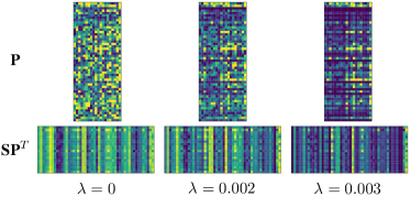
Figure 2: Visualizations of the learned matrix $\textbf{P}\in\mathbb{R}^{d\times k}$ and $\textbf{S}\textbf{P}^{T}\in\mathbb{R}^{n\times d}$ under different $\lambda$. We set the prompt basis vector number $k=20$, feature dimension $d=50$, and the node number $n=20$ for demonstration. Here, we can note that, as the parameter $\lambda$ increases, there are more zero rows in P and thus more zero columns in $\textbf{S}\textbf{P}^{T}$.

V Optimization

In this section, we propose a simple yet effective algorithm to optimize the above GSFPs (GSFP, GSmFP). The proposed GSFPs involve $\ell_{1}$ and $\ell_{2,1}$ norm regularization terms, which are difficult to employ gradient descent to optimize them directly. In this paper, we propose to utilize the Forward-backward splitting method [32] to optimize them.

V-A Optimization of GSFP

Our GSFP problem Eq.(7) has two learnable parameters, i.e., prompt p and task head parameters $\theta$. In the following, we introduce the detailed optimization algorithms for them respectively.

Optimize p: We adopt the Forward-backward splitting scheme to optimize prompt p in GSFP problem Eq.(7). It conducts the optimization via the following update rule,

$$\textbf{p}\leftarrow\text{Prox1}_{\lambda}\left(\textbf{p}-\eta\nabla_{\textbf{p}}\mathcal{L}^{{down}}\right)$$ (9)

where $\eta$ denotes the learning rate and $\lambda$ is the penalty parameter in Eq.(7). The proximal operator Prox1 is defined as follows,

$$\text{Prox1}_{\lambda}(\textbf{y})=\underset{\textbf{z}}{\arg\min}\,\,\frac{1}{2}\|\textbf{z}-\textbf{y}\|_{2}^{2}+\lambda\|\textbf{z}\|_{1}$$ (10)

It is known that problem Eq.(10) has the closed-form solution as,

$$\textbf{z}_{i}^{*}=\text{sign}(\textbf{y}_{i})\max\big{(}|\textbf{y}_{i}|-\lambda,0\big{)}$$ (11)

where $\textbf{z}_{i}^{*}$ and $\textbf{y}_{i}$ represent the $i$-th element of vector $\textbf{z}^{*}$ and y, respectively.

Optimize $\theta$: The optimal $\theta^{*}$ is obtained by using gradient descent strategy, as commonly employed in many other works [13, 10]. The whole algorithm is summarized in Algorithm 1.

V-B Optimization of GSmFP

For GSmFP, we can also employ the Forward-backward splitting method to optimize prompt matrix P and use gradient descent strategy to optimize $\theta$. Specifically, the update rule for optimizing P is given as,

$$\textbf{P}\leftarrow\text{Prox21}_{\lambda}\left(\textbf{P}-\eta\nabla_{\textbf{P}}\mathcal{L}^{{down}}\right)$$ (12)

where $\eta$ is the learning rate and $\lambda$ is the penalty parameter in Eq.(8). The proximal operator Prox21 is defined as,

$$\text{Prox21}_{\lambda}(\textbf{Y})=\underset{\textbf{Z}}{\arg\min}\,\,\frac{1}{2}\|\textbf{Z}-\textbf{Y}\|_{F}^{2}+\lambda\|\textbf{Z}\|_{2,1}$$ (13)

It is known that problem Eq.(13) has the closed-form solution which is given as,

$$\textbf{Z}_{i}^{*}=\begin{cases}\begin{aligned} &\frac{\|\textbf{Y}_{i}\|_{2}-\lambda}{\|\textbf{Y}_{i}\|_{2}}\textbf{Y}_{i},\quad&&\text{if }\lambda<\|\textbf{Y}_{i}\|_{2}\\ &\textbf{0},\quad&&\text{otherwise}\end{aligned}\end{cases}$$ (14)

where $\textbf{Z}_{i}^{*}$ and $\textbf{Y}_{i}$ represent the $i$-th row of the matrix $\textbf{Z}^{*}$ and Y, respectively. The whole algorithm is summarized in Algorithm 2. Figure 3 shows the training loss curves of GSFP and GSmFP on Cora [33] and CiteSeer [33] datasets, demonstrating the convergence of the above Algorithm 1 and 2.

Algorithm 1 Optimization of GSFP

  Input: An input graph $\mathcal{G}(\textbf{X},\textbf{A})$, learning rate $\eta$ and penalty parameter $\lambda$

  Output: Optimal prompt vector $\textbf{p}^{*}$ and parameters $\theta^{*}$

  Initialize p and $\theta$

  while not converged do

     $\textbf{p}\leftarrow\textbf{p}-\eta\nabla_{\textbf{p}}\mathcal{L}^{{down}}$

     $\textbf{p}\leftarrow\text{Prox1}_{\lambda}(\textbf{p})$

     $\theta\leftarrow\theta-\eta\nabla_{\theta}\mathcal{L}^{{down}}$

  end while

  Return: $\textbf{p}^{*}$, $\theta^{*}$

Algorithm 2 Optimization of GSmFP

  Input: An input graph $\mathcal{G}(\textbf{X},\textbf{A})$, learning rate $\eta$ and penalty parameter $\lambda$

  Output: Optimal prompt matrix $\textbf{P}^{*}$ and parameters $\theta^{*}$

  Initialize P and $\theta$

  while not converged do

     $\textbf{P}\leftarrow\textbf{P}-\eta\nabla_{\textbf{P}}\mathcal{L}^{{down}}$

     $\textbf{P}\leftarrow\text{Prox21}_{\lambda}\left(\textbf{P}\right)$

     $\theta\leftarrow\theta-\eta\nabla_{\theta}\mathcal{L}^{{down}}$

  end while

  Return: $\textbf{P}^{*}$, $\theta^{*}$

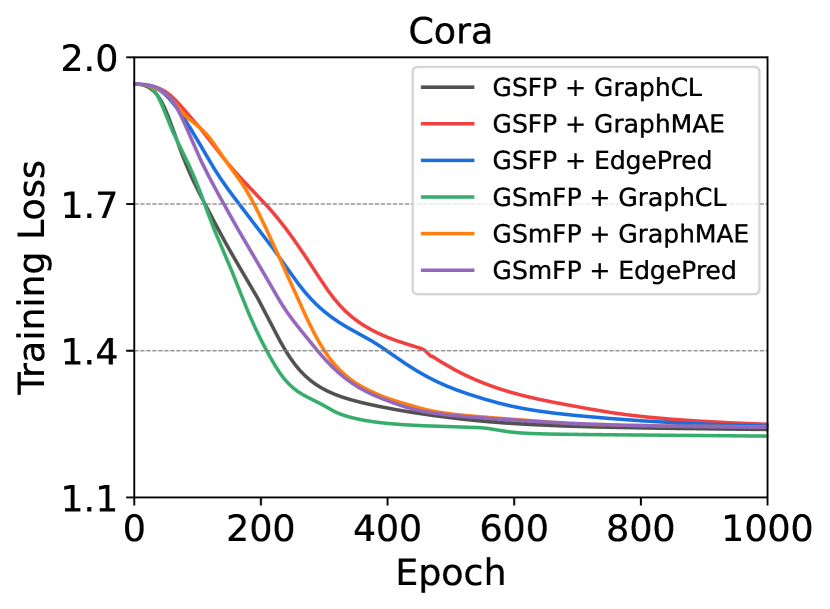
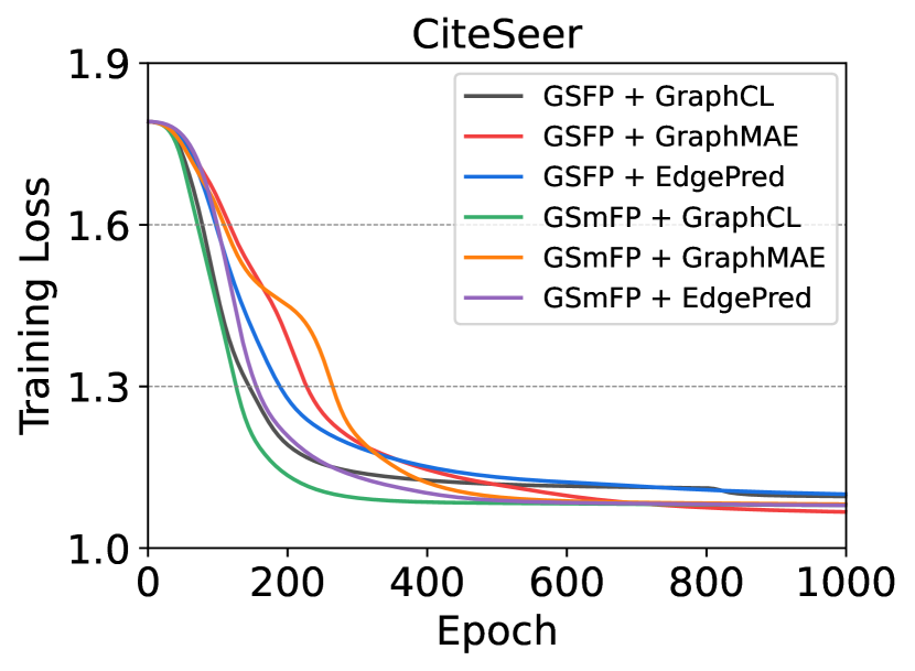
Figure 3: Training loss curves on Cora and CiteSeer datasets.

TABLE I: Statistics of datasets.

Dataset	Graphs	Avg.nodes	Avg.edges	Features	Classes
Cora	1	2,708	10,556	1,433	7
CiteSeer	1	3,327	9,104	3,703	6
PubMed	1	19,717	88,648	500	3
Photo	1	7,650	238,162	745	8
Computers	1	13,752	491,722	767	10
CS	1	18,333	163,788	6,805	15
Physics	1	34,493	495,924	8,415	5
Wisconsin	1	251	515	1,703	5
Cornell	1	183	298	1,703	5
Chameleon	1	2,277	62,792	2,325	5
Ogbn-arxiv	1	169,343	1,166,243	128	40
COX2	467	41.22	43.45	3	2
MUTAG	188	17.93	19.79	7	2
IMDB-BINARY	1,000	19.77	96.53	0	2
IMDB-MULTI	1,500	13.00	65.94	0	3
REDDIT-MULTI-5K	4,999	508.52	594.87	0	5

VI Experiment

VI-A Experimental Setup

Datasets. To evaluate our proposed GSFP and GSmFP, we conduct experiments on 16 widely-used benchmark datasets on both node classification and graph classification tasks. For node classification task, we use eleven datasets including three citation networks (Cora [33], CiteSeer [33], PubMed [33]), two Amazon co-purchase datasets (Amazon Photo [34], Amazon Computers [34]), two co-author networks (Coauthor CS [35], Coauthor Physics [35]), three heterophilic web page networks (Wisconsin [36], Cornell [36], Chameleon [36]) and one large-scale dataset (Ogbn-arxiv [37]). For graph classification task, we use five datasets including two molecule datasets (COX2 [38], MUTAG [39]), two movie collaboration datasets (IMDB-BINARY [40], IMDB-MULTI [40]) and one social network dataset (REDDIT-MULTI-5K [40]). The detailed descriptions of these datasets are summarized in Table I. Similar to works [41, 42], we adopt 1-shot setting for training and split the remaining samples into validation and test sets at a 1:9 ratio.

Baselines. We compare our methods with three kinds of approaches: (1) Supervised method: We choose GCN [43] as the backbone network under supervised setting for the comparison. (2) ‘Pre-training + fine-tuning’ methods: GraphMAE [21] leverages a masked autoencoder to learn node representations by reconstructing the masked features. EdgePred [8] randomly drops a portion of edges and trains the GNN model to reconstruct them. GraphCL [23] employs contrastive learning to maximize the agreement between different augmented views of the same graph. (3) Prompt learning methods: We select several mainstream prompt learning methods including All-in-One [10], GPF [13], GPF-plus [13], GraphPrompt [9] and GPPT [8]. All-in-One concatenates the input graph with the prompt graph. Both GPF and GPF-plus add prompt vectors to the input features. GraphPrompt uses a prompt vector to assist the readout operation. GPPT transforms the node classification task into the link prediction pre-training via prompt tokens.

Implementation details. We conduct all experiments based on ProG library [41]. For a fair comparison, we use a 3-layer GCN [43] architecture with a hidden dimension of 256 for all methods. For all pre-training methods, we pre-train the model on Flickr [44] dataset and then fine-tune it on other node classification datasets. Therefore, we apply a learnable linear transformation to unify all feature dimensions to 100. Similarly, for graph classification task, we pre-train the model on DD [45] dataset and then fine-tune it on other graph classification datasets.

Parameter setup. During the pre-training phase, the learning rate is set to 1e-3 and the weight decay is set to 1e-5. For downstream tasks, we set the learning rate to 1e-3 and the weight decay to 5e-4 for all methods. For other parameters in the comparison methods, we generally follow the default parameters in the original publications. For GPF-plus [13] and our GSmFP, $k$ is set to 10 and 20 respectively for node classification and graph classification task. Besides, we determine the optimal parameter $\lambda$ values based on the performance on validation set.

TABLE III: Accuracy of 1-shot graph classification.

Method \Dataset		COX2	MUTAG	IMDB-B	IMDB-M	RDT-M5K
GCN		63.87±6.69	55.95±13.59	50.08±0.72	36.94±2.71	21.99±3.02
EdgePred	FT	60.76±2.84	53.10±17.28	55.68±7.19	34.35±5.79	22.53±2.86
	All-in-One	60.43±7.59	62.02±14.10	61.71±5.26	36.22±5.97	26.20±4.21
	GPF	60.81±4.03	56.43±15.44	62.14±5.18	37.18±6.46	23.29±0.92
	GPF-plus	56.47±9.08	57.98±11.48	60.87±4.71	37.98±5.67	24.48±3.19
	GSFP	64.73±7.69	58.45±12.88	64.45±2.13	38.04±4.63	23.37±2.64
	GSmFP	62.20±10.06	58.69±10.84	62.65±6.74	40.86±3.39	25.78±7.47
GraphCL	FT	62.63±5.58	55.71±13.55	50.06±0.72	33.95±1.20	22.09±2.40
	All-in-One	57.85±7.20	64.52±19.22	59.38±5.64	36.57±4.38	22.67±3.67
	GPF	63.48±4.96	55.83±14.05	62.14±5.12	37.77±5.44	23.46±4.12
	GPF-plus	61.24±4.34	53.81±17.65	61.74±5.70	37.91±5.49	25.86±4.77
	GSFP	63.34±6.94	58.10±13.23	63.45±2.80	38.19±5.31	24.31±3.85
	GSmFP	63.58±7.01	55.83±12.45	65.05±1.13	39.07±6.09	26.13±4.94
GraphMAE	FT	59.76±7.24	49.76±15.85	52.41±6.01	32.95±0.29	22.60±2.73
	All-in-One	55.32±27.44	65.71±25.80	61.47±3.28	37.05±6.31	22.81±3.61
	GPF	57.66±6.04	59.64±14.80	62.16±4.92	36.91±6.96	23.39±0.90
	GPF-plus	64.15±7.37	52.98±19.15	61.22±4.60	37.33±6.94	23.19±0.91
	GSFP	63.39±9.17	59.29±14.01	63.36±3.89	37.12±7.00	23.91±2.01
	GSmFP	66.06±7.55	58.93±14.19	62.45±3.51	37.77±7.67	23.01±0.74
GraphPrompt		61.19±6.48	54.05±16.02	58.20±4.88	34.84±3.87	23.86±1.44

TABLE II: Accuracy of 1-shot node classification.

Method \Dataset		Cora	CiteSeer	PubMed	Photo	Computers	CS	Physics	Wisconsin	Cornell	Chameleon	Ogbn-arxiv
GCN		29.84±9.15	27.63±6.36	51.52±10.97	39.45±8.54	34.94±11.03	57.43±7.86	53.05±21.47	20.18±5.20	23.98±6.50	22.39±1.61	5.27±2.18
EdgePred	FT	31.11±6.41	26.92±4.20	51.17±11.69	40.81±5.73	33.47±11.21	55.49±7.13	52.67±19.07	23.69±3.27	22.24±6.77	25.14±3.57	6.04±2.18
	All-in-One	20.44±8.12	19.73±2.37	42.08±7.82	34.04±5.25	27.84±6.73	36.41±4.41	43.22±9.15	21.26±9.31	16.15±7.20	21.90±1.67	0.95±1.26
	GPF	35.16±12.74	33.19±5.04	48.14±7.67	46.79±6.65	39.58±11.52	64.89±8.79	66.48±20.03	25.59±10.41	25.22±8.26	22.61±2.46	10.30±3.43
	GPF-plus	34.04±11.06	33.46±4.60	47.07±7.49	47.52±5.66	37.36±9.09	62.96±9.25	70.36±18.10	27.57±9.38	24.72±8.65	23.05±2.80	9.58±2.60
	GSFP	36.07±13.60	33.20±6.82	51.35±10.72	48.00±4.86	42.16±9.30	65.61±8.60	73.70±19.15	25.50±10.19	25.47±8.63	22.67±2.32	11.17±3.81
	GSmFP	36.03±13.14	33.52±4.76	51.90±12.52	49.56±7.07	43.21±8.93	64.11±10.59	74.17±17.08	27.57±9.17	24.97±8.08	22.86±2.67	10.24±2.69
GraphCL	FT	30.89±8.66	28.52±6.26	48.80±7.42	36.98±7.21	31.69±5.00	54.37±5.66	64.65±14.07	20.54±12.53	26.21±7.62	24.11±3.01	4.76±1.21
	All-in-One	14.70±7.43	20.61±1.21	41.45±6.49	29.52±1.58	24.34±5.63	35.27±4.51	43.80±8.16	25.68±14.77	18.63±11.21	21.71±1.24	3.09±4.83
	GPF	33.24±13.86	32.77±5.44	48.25±7.84	43.28±5.53	34.52±8.45	61.83±6.64	69.59±16.99	26.04±9.18	23.48±5.87	23.70±3.58	6.24±1.52
	GPF-plus	32.68±10.75	27.86±5.94	48.21±8.21	42.64±8.07	33.46±7.10	56.97±7.56	69.83±15.56	26.04±8.66	25.09±8.10	23.61±3.21	7.38±2.14
	GSFP	33.20±13.85	33.08±5.70	53.56±10.36	49.56±8.73	38.46±11.05	63.41±9.54	74.62±14.92	27.57±8.14	25.71±6.47	25.45±3.94	9.35±2.49
	GSmFP	34.08±13.43	33.60±5.75	55.74±13.36	46.71±8.34	36.60±7.89	60.43±6.37	72.83±16.55	25.68±9.20	25.59±8.03	26.81±1.30	9.12±2.17
GraphMAE	FT	30.49±9.08	31.40±5.29	49.93±9.62	40.54±11.22	32.79±10.00	54.99±7.46	46.88±16.11	20.09±4.55	24.47±7.09	23.64±2.86	5.15±2.93
	All-in-One	12.54±2.52	20.71±1.46	39.82±9.14	42.56±7.47	31.32±9.30	37.39±5.00	39.74±10.10	24.14±13.95	20.62±10.51	21.65±1.45	3.09±4.83
	GPF	35.15±12.96	32.77±5.86	48.11±7.79	46.44±7.37	39.24±10.32	63.31±10.46	75.28±15.69	24.05±10.04	24.35±8.16	22.55±2.44	9.11±2.40
	GPF-plus	34.05±9.41	31.05±5.50	48.47±7.49	46.41±6.39	39.73±11.91	65.30±8.81	69.71±17.24	27.03±9.31	24.60±8.72	23.55±3.42	7.72±1.23
	GSFP	38.56±8.96	34.61±6.90	50.74±8.61	49.53±4.58	41.21±10.80	64.81±9.78	75.32±15.57	25.14±9.83	25.09±9.09	22.57±2.46	10.81±3.88
	GSmFP	39.29±7.79	33.61±5.30	50.70±8.78	49.99±5.75	42.89±10.71	65.33±8.82	75.37±17.64	27.12±9.77	25.34±7.97	25.16±2.98	10.65±0.70
GPPT		20.11±8.82	26.07±6.36	59.93±7.30	58.62±9.27	37.89±12.82	62.40±7.16	84.91±3.34	23.15±6.09	22.98±9.61	24.16±4.14	5.62±4.29
GraphPrompt		34.88±10.64	25.67±4.40	46.02±6.72	47.10±6.83	34.07±7.81	61.03±10.52	69.02±4.90	21.53±5.61	24.97±8.06	22.88±2.37	9.55±2.94

VI-B Comparison Results

Node classification. In Table II, we show the results of all methods with five random splits under the 1-shot setting. One can observe that (1) Compared to traditional ‘pre-training + fine-tuning’ methods, most graph prompt learning methods obtain better results, which indicates that prompt learning can effectively mitigate the negative transfer issue caused by the task and graph domain gap between the pre-training and downstream stages. (2) The proposed GSFP and GSmFP gain significant improvements over GPF [13] and GPF-plus [13] which also conduct prompting on node features. This validates the effectiveness of the proposed GSFPs which conduct prompting on specific node feature dimensions and thus perform more optimally and reliably. (3) Our methods can obtain the best (or 2nd best) performance on all datasets, which further demonstrates the superiority of GSFP and GSmFP.

Graph classification. In Table III, we show the results of all methods under the 1-shot setting on five graph classification datasets. One can note that the proposed GSFP and GSmFP perform better than GPF [13] and GPF-plus [13] in most cases, which is consistent with the results in Table II. Besides, our methods almost achieve the best results on all datasets, which further shows the effectiveness of the proposed methods on graph classification task.

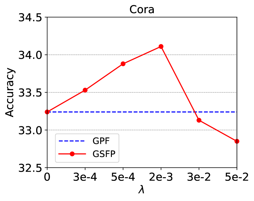
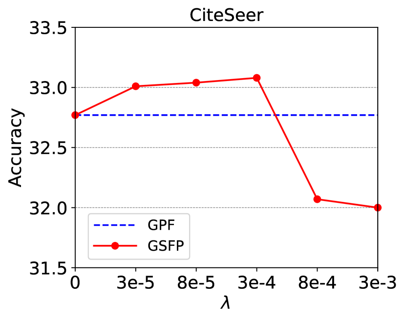
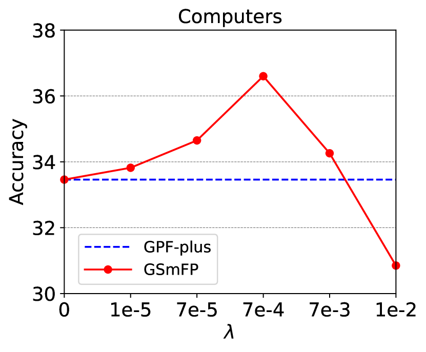
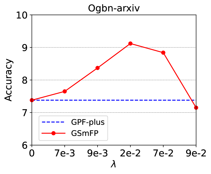
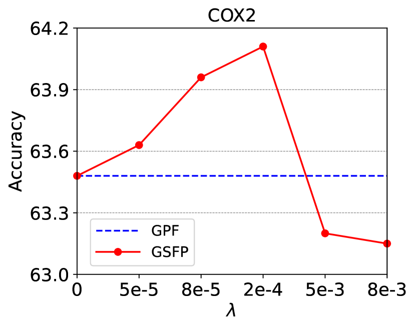
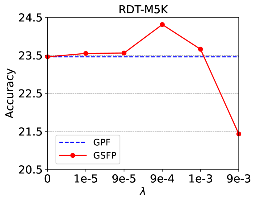
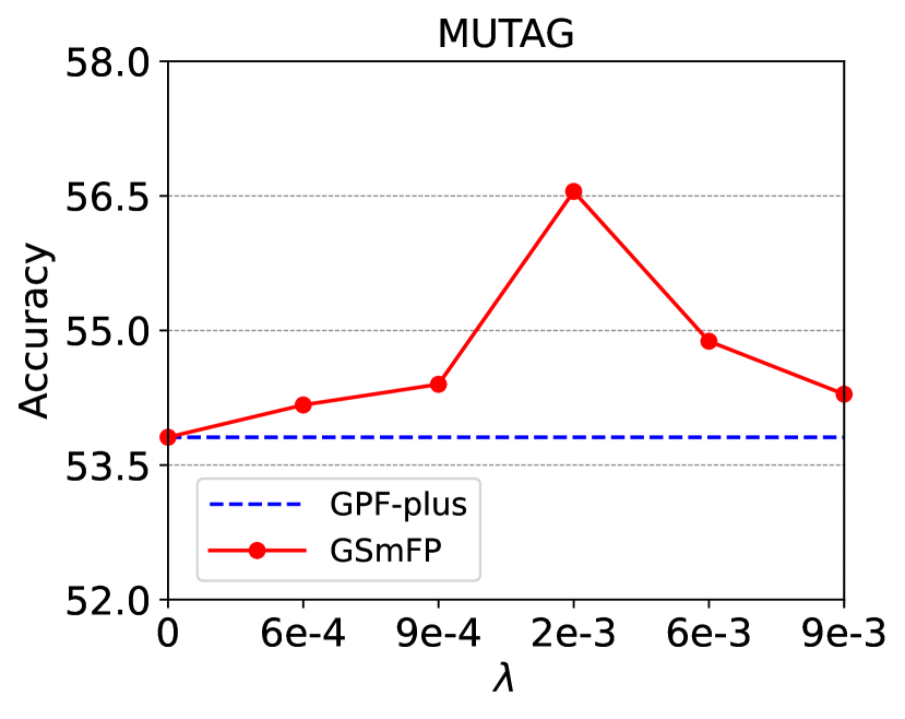
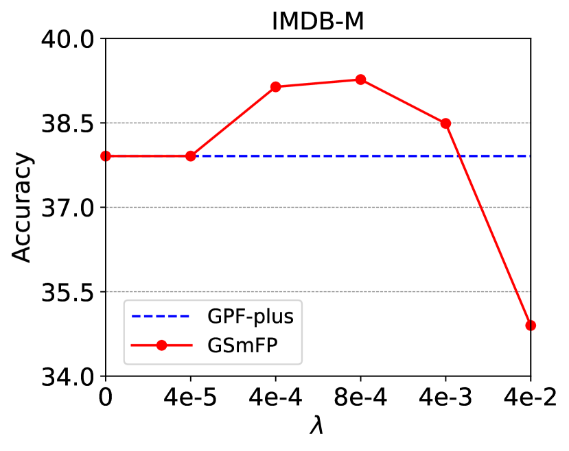
Figure 4: Analyze the impact of parameter $\lambda$ on different datasets.

VI-C Parameter Analysis

As mentioned in Section IV, the parameter $\lambda$ controls the sparsity of the learned prompt. Thus, we analyze the effect of different $\lambda$ values on performance. Note that when $\lambda=0$, the proposed GSFP and GSmFP degrade to GPF [13] and GPF-plus [13], respectively. As shown in Figure 4, one can see that our methods achieve better performance than the baseline ($\lambda=0$) within a certain range. Besides, as $\lambda$ continues to increase, prompting can only be conducted on very few or no feature dimensions, which leads to a performance drop. This demonstrates the effectiveness of conducting prompting selectively on specific feature dimensions.

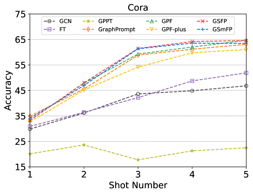
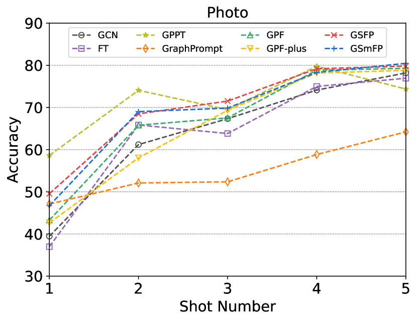
Figure 5: Analyze the impact of different shot numbers on Cora and Photo datasets.

TABLE IV: Performance on different backbones.

Dataset		Cora		Photo
Method \Backbone		GAT	SAGE	GAT	SAGE
Supervised		32.26±7.99	22.06±6.10	37.08±8.20	38.78±10.02
GraphCL	FT	33.92±7.33	30.30±7.82	30.75±11.67	34.28±5.24
	All-in-One	21.97±11.92	37.49±9.25	26.14±5.45	29.60±6.72
	GPF	33.32±9.14	34.01±9.97	36.71±4.51	37.06±2.48
	GPF-plus	36.25±6.62	32.47±6.95	33.37±2.93	34.51±8.19
	GSFP	36.64±10.03	35.77±10.17	38.57±11.16	37.93±3.47
	GSmFP	36.67±6.29	33.23±6.51	38.01±5.60	39.54±5.02
GraphMAE	FT	35.70±9.54	20.68±7.43	36.32±7.15	35.09±4.06
	All-in-One	19.98±8.44	15.28±3.81	26.48±5.05	39.95±6.37
	GPF	35.18±11.20	37.71±6.15	33.91±5.08	46.13±4.83
	GPF-plus	34.32±8.35	36.65±10.55	37.06±6.10	45.55±4.62
	GSFP	38.79±9.22	38.00±5.91	43.31±6.74	47.67±4.28
	GSmFP	37.32±8.16	36.68±10.52	40.95±8.80	48.08±5.55
GPPT		31.04±15.07	20.67±4.06	48.48±4.00	53.86±10.73
GraphPrompt		37.93±12.16	35.95±9.68	47.61±3.64	48.08±11.85

VI-D Additional Experiments

Impact of different shot numbers. Figure 5 shows the performance across different shot numbers on Cora [33] and Photo [34] datasets. One can observe that most methods show improved performance with the increasing shot number. Our GSFP and GSmFP obtain a better advantage in most cases.

Performance on different backbones. Table IV shows the results of using GAT [46] and GraphSAGE [47] as backbones on Cora [33] and Photo [34] datasets. Here, GSFP and GSmFP obtain improvements compared to GPF [13] and GPF-plus [13], and they are also competitive with other comparison methods. This further demonstrates the generality and advantage of our GSFP methods on different GNN backbones.

VII Conclusion

This paper first arises a new graph prompting problem, termed Graph Sparse Prompting (GSP), which is defined as adaptively and sparsely selecting the optimal graph elements (this paper focuses on node attributes) to achieve compact prompting for downstream tasks. Then, we propose two kinds of graph sparse prompting over attributes, termed GSFP and GSmFP, by leveraging sparsity-inducing constraint/regularization into the graph prompt optimization objective. We derive an effective algorithm to optimize them. Experiments on many benchmark datasets demonstrate that the proposed GSFPs outperform many other comparison baselines on several pre-trained GNNs and different downstream tasks.

References

- [1] X. Li, L. Sun, M. Ling, and Y. Peng, “A survey of graph neural network based recommendation in social networks,” Neurocomputing, vol. 549, p. 126441, 2023.
- [2] J. Xiong, Z. Xiong, K. Chen, H. Jiang, and M. Zheng, “Graph neural networks for automated de novo drug design,” Drug Discovery Today, vol. 26, no. 6, pp. 1382–1393, 2021.
- [3] Y. Liu, X. Ao, Z. Qin, J. Chi, J. Feng, H. Yang, and Q. He, “Pick and choose: A gnn-based imbalanced learning approach for fraud detection,” in Proceedings of the Web Conference 2021, p. 3168–3177, 2021.
- [4] L. Kong, H. Yang, W. Li, J. Guan, and S. Zhou, “Traffexplainer: A framework towards gnn-based interpretable traffic prediction,” IEEE Transactions on Artificial Intelligence, pp. 1–15, 2024.
- [5] Y. Xie, Z. Xu, J. Zhang, Z. Wang, and S. Ji, “Self-supervised learning of graph neural networks: A unified review,” IEEE Transactions on Pattern Analysis and Machine Intelligence, vol. 45, no. 2, pp. 2412–2429, 2023.
- [6] L. Wang, M. Zhang, Z. Jia, Q. Li, C. Bao, K. Ma, J. Zhu, and Y. Zhong, “Afec: Active forgetting of negative transfer in continual learning,” Advances in Neural Information Processing Systems, vol. 34, pp. 22379–22391, 2021.
- [7] X. Sun, J. Zhang, X. Wu, H. Cheng, Y. Xiong, and J. Li, “Graph prompt learning: A comprehensive survey and beyond,” arXiv:2311.16534, 2023.
- [8] M. Sun, K. Zhou, X. He, Y. Wang, and X. Wang, “Gppt: Graph pre-training and prompt tuning to generalize graph neural networks,” in Proceedings of the 28th ACM SIGKDD Conference on Knowledge Discovery and Data Mining, p. 1717–1727, 2022.
- [9] Z. Liu, X. Yu, Y. Fang, and X. Zhang, “Graphprompt: Unifying pre-training and downstream tasks for graph neural networks,” in Proceedings of the ACM Web Conference 2023, p. 417–428, 2023.
- [10] X. Sun, H. Cheng, J. Li, B. Liu, and J. Guan, “All in one: Multi-task prompting for graph neural networks,” in Proceedings of the 29th ACM SIGKDD Conference on Knowledge Discovery and Data Mining, p. 2120–2131, 2023.
- [11] Y. Guo, C. Yang, Y. Chen, J. Liu, C. Shi, and J. Du, “A data-centric framework to endow graph neural networks with out-of-distribution detection ability,” in Proceedings of the 29th ACM SIGKDD Conference on Knowledge Discovery and Data Mining, p. 638–648, 2023.
- [12] Q. Ge, Z. Zhao, Y. Liu, A. Cheng, X. Li, S. Wang, and D. Yin, “Psp: Pre-training and structure prompt tuning for graph neural networks,” in Joint European Conference on Machine Learning and Knowledge Discovery in Databases, p. 423–439, 2024.
- [13] T. Fang, Y. Zhang, Y. YANG, C. Wang, and L. Chen, “Universal prompt tuning for graph neural networks,” in Advances in Neural Information Processing Systems, vol. 36, pp. 52464–52489, 2023.
- [14] J. Lee, W. Yang, and J. Kang, “Subgraph-level universal prompt tuning,” arXiv preprint arXiv:2402.10380, 2024.
- [15] B. Jiang, H. Wu, Z. Zhang, B. Wang, and J. Tang, “A unified graph selective prompt learning for graph neural networks,” arXiv preprint arXiv:2406.10498, 2024.
- [16] Z. Tan, R. Guo, K. Ding, and H. Liu, “Virtual node tuning for few-shot node classification,” in Proceedings of the 29th ACM SIGKDD Conference on Knowledge Discovery and Data Mining, p. 2177–2188, 2023.
- [17] Q. Wang, X. Sun, and H. Cheng, “Does graph prompt work? a data operation perspective with theoretical analysis,” arXiv preprint arXiv:2410.01635, 2024.
- [18] F. Nie, H. Huang, X. Cai, and C. Ding, “Efficient and robust feature selection via joint -norms minimization,” in Advances in Neural Information Processing Systems, vol. 23, pp. 1813–1821, 2010.
- [19] J. Wright, A. Y. Yang, A. Ganesh, S. S. Sastry, and Y. Ma, “Robust face recognition via sparse representation,” IEEE Transactions on Pattern Analysis and Machine Intelligence, vol. 31, no. 2, pp. 210–227, 2009.
- [20] P. Veličković, W. Fedus, W. L. Hamilton, P. Liò, Y. Bengio, and R. D. Hjelm, “Deep graph infomax,” in International Conference on Learning Representations, 2019.
- [21] Z. Hou, X. Liu, Y. Cen, Y. Dong, H. Yang, C. Wang, and J. Tang, “Graphmae: Self-supervised masked graph autoencoders,” in Proceedings of the 28th ACM SIGKDD Conference on Knowledge Discovery and Data Mining, p. 594–604, 2022.
- [22] T. N. Kipf and M. Welling, “Variational graph auto-encoders,” NeurIPS Workshop on Bayesian Deep Learning, 2016.
- [23] Y. You, T. Chen, Y. Sui, T. Chen, Z. Wang, and Y. Shen, “Graph contrastive learning with augmentations,” in Advances in Neural Information Processing Systems, vol. 33, pp. 5812–5823, 2020.
- [24] J. Xia, L. Wu, J. Chen, B. Hu, and S. Z. Li, “Simgrace: A simple framework for graph contrastive learning without data augmentation,” in Proceedings of the ACM Web Conference 2022, p. 1070–1079, 2022.
- [25] W. Jin, T. Derr, H. Liu, Y. Wang, S. Wang, Z. Liu, and J. Tang, “Self-supervised learning on graphs: Deep insights and new direction,” arXiv preprint arXiv:2006.10141, 2020.
- [26] Q. Huang, H. Ren, P. Chen, G. Kržmanc, D. Zeng, P. S. Liang, and J. Leskovec, “Prodigy: Enabling in-context learning over graphs,” in Advances in Neural Information Processing Systems, vol. 36, pp. 16302–16317, 2023.
- [27] H. Liu, J. Feng, L. Kong, N. Liang, D. Tao, Y. Chen, and M. Zhang, “One for all: Towards training one graph model for all classification tasks,” in The Twelfth International Conference on Learning Representations, 2024.
- [28] Y. Ma, N. Yan, J. Li, M. Mortazavi, and N. V. Chawla, “Hetgpt: Harnessing the power of prompt tuning in pre-trained heterogeneous graph neural networks,” in Proceedings of the ACM Web Conference 2024, p. 1015–1023, 2024.
- [29] X. Yu, Y. Fang, Z. Liu, and X. Zhang, “Hgprompt: Bridging homogeneous and heterogeneous graphs for few-shot prompt learning,” in Proceedings of the AAAI Conference on Artificial Intelligence, vol. 38, pp. 16578–16586, 2024.
- [30] X. Yu, C. Zhou, Y. Fang, and X. Zhang, “Text-free multi-domain graph pre-training: Toward graph foundation models,” arXiv preprint arXiv:2405.13934, 2024.
- [31] R. Tibshirani, “Regression shrinkage and selection via the lasso,” Journal of the Royal Statistical Society Series B: Statistical Methodology, vol. 58, no. 1, pp. 267–288, 1996.
- [32] P. L. Combettes and J.-C. Pesquet, “Proximal splitting methods in signal processing,” Fixed-Point Algorithms for Inverse Problems in Science and Engineering, pp. 185–212, 2011.
- [33] P. Sen, G. Namata, M. Bilgic, L. Getoor, B. Galligher, and T. Eliassi-Rad, “Collective classification in network data,” AI magazine, vol. 29, no. 3, pp. 93–93, 2008.
- [34] O. Shchur, M. Mumme, A. Bojchevski, and S. Günnemann, “Pitfalls of graph neural network evaluation,” NeurIPS Workshop on Relational Representation Learning, 2018.
- [35] A. Sinha, Z. Shen, Y. Song, H. Ma, D. Eide, B.-J. P. Hsu, and K. Wang, “An overview of microsoft academic service (mas) and applications,” in Proceedings of the 24th International Conference on World Wide Web, p. 243–246, 2015.
- [36] H. Pei, B. Wei, K. C.-C. Chang, Y. Lei, and B. Yang, “Geom-gcn: Geometric graph convolutional networks,” in International Conference on Learning Representations, 2020.
- [37] W. Hu, M. Fey, M. Zitnik, Y. Dong, H. Ren, B. Liu, M. Catasta, and J. Leskovec, “Open graph benchmark: Datasets for machine learning on graphs,” in Advances in Neural Information Processing Systems, vol. 33, pp. 22118–22133, 2020.
- [38] R. A. Rossi and N. K. Ahmed, “The network data repository with interactive graph analytics and visualization,” in Proceedings of the Twenty-Ninth AAAI Conference on Artificial Intelligence, p. 4292–4293, 2015.
- [39] N. Kriege and P. Mutzel, “Subgraph matching kernels for attributed graphs,” in Proceedings of the 29th International Coference on International Conference on Machine Learning, p. 291–298, 2012.
- [40] P. Yanardag and S. Vishwanathan, “Deep graph kernels,” in Proceedings of the 21th ACM SIGKDD International Conference on Knowledge Discovery and Data Mining, p. 1365–1374, 2015.
- [41] C. Zi, H. Zhao, X. Sun, Y. Lin, H. Cheng, and J. Li, “Prog: A graph prompt learning benchmark,” Advances in Neural Information Processing Systems, 2024.
- [42] H. Zhao, A. Chen, X. Sun, H. Cheng, and J. Li, “All in one and one for all: A simple yet effective method towards cross-domain graph pretraining,” p. 4443–4454, 2024.
- [43] T. N. Kipf and M. Welling, “Semi-supervised classification with graph convolutional networks,” in International Conference on Learning Representations, 2017.
- [44] H. Zeng, H. Zhou, A. Srivastava, R. Kannan, and V. Prasanna, “Graphsaint: Graph sampling based inductive learning method,” in International Conference on Learning Representations, 2020.
- [45] P. D. Dobson and A. J. Doig, “Distinguishing enzyme structures from non-enzymes without alignments,” Journal of Molecular Biology, vol. 330, no. 4, pp. 771–783, 2003.
- [46] P. Veličković, G. Cucurull, A. Casanova, A. Romero, P. Liò, and Y. Bengio, “Graph attention networks,” in International Conference on Learning Representations, 2018.
- [47] W. Hamilton, Z. Ying, and J. Leskovec, “Inductive representation learning on large graphs,” in Advances in Neural Information Processing Systems, vol. 30, pp. 1024–1034, 2017.