Generating Realistic Tabular Data with Large Language Models
Abstract
While most generative models show achievements in image data generation, few are developed for tabular data generation. Recently, due to success of large language models (LLM) in diverse tasks, they have also been used for tabular data generation. However, these methods do not capture the correct correlation between the features and the target variable, hindering their applications in downstream predictive tasks. To address this problem, we propose a LLM-based method with three important improvements to correctly capture the ground-truth feature-class correlation in the real data. First, we propose a novel permutation strategy for the input data in the fine-tuning phase. Second, we propose a feature-conditional sampling approach to generate synthetic samples. Finally, we generate the labels by constructing prompts based on the generated samples to query our fine-tuned LLM. Our extensive experiments show that our method significantly outperforms 10 SOTA baselines on 20 datasets in downstream tasks. It also produces highly realistic synthetic samples in terms of quality and diversity. More importantly, classifiers trained with our synthetic data can even compete with classifiers trained with the original data on half of the benchmark datasets, which is a significant achievement in tabular data generation.
I Introduction
Recently, tabular data generation has attracted a significant attention from the research community as synthetic data can improve different aspects of training data such as privacy [40], quality [43], fairness [34], and availability [25]. Particularly noteworthy is its capacity to overcome usage restrictions while preserving privacy e.g. synthetic data replace real data in training machine learning (ML) models [44, 7].
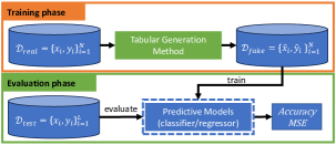
To evaluate an image generation method, we often generate synthetic images , and visualize to assess whether they are naturally good looking [18]. However, since it is hard to say whether a synthetic tabular sample looks real or fake with bare eyes, evaluating a tabular generation method often follows the “train on synthetic, test on real (TSTR)” approach [12, 19]. It is a common practice to generate synthetic samples and their labels , then use them to train ML predictive models and compute performance scores on a real test set. A better score means a better tabular generation method. Figure 1 illustrates the training and evaluation phases.
Among existing approaches, generative adversarial network (GAN)-based methods are widely used for tabular data generation [10, 37, 30, 44, 3, 21]. Recently, large language models (LLM)-based methods are proposed, and they show promising results [7, 48]. Compared to GAN-based methods, LLM-based methods have some advantages. First, since they do not require heavy data pre-processing steps e.g. encoding categorical data or normalizing continuous data, they avoid information loss and artificial introduction. Second, since they represent tabular data as text instead of numerical, they can capture the context knowledge among variables e.g. the relationship between Age and Marriage.
To generate a sample that has features and a label , most existing methods treat the target variable as a regular feature [37, 44, 21, 7]. However, these methods may not correctly capture the correlation between and , which is very important for training predictive models in the evaluation phase (see Figure 1). Some methods generate only , and use an external classifier trained on the real dataset to predict [48]. However, this method is cumbersome since it needs two standalone models – a generative model and a predictive model. As shown in Figure 2, we compute the importance level of each feature for each class on the dataset Cardiotocography using the Shapley values [24]. We compare the feature importance on the original data with the feature importance on the synthetic data generated by various methods. Existing state-of-the-art methods such as TVAE [44], CTGAN [44], Great [7], and TapTap [48] cannot capture the ground-truth feature-class correlation on the real dataset. This suggests that the data generated with these methods does not closely mimic the real data.
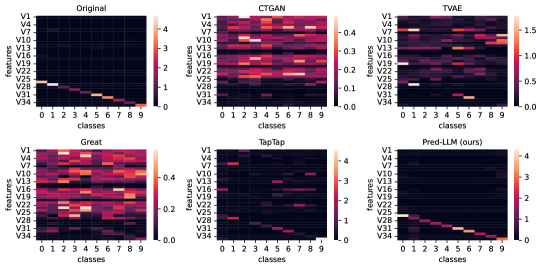
To address the problem, we propose a LLM-based method with three improvements. First, we observe that existing LLM-based methods permute both the features and the target variable in the fine-tuning phase to support arbitrary conditioning i.e. the capacity to generate data conditioned on an arbitrary set of variables. However, this way has a significant disadvantage. In the attention matrix of LLM, each token only pays attention to every token before it, but not any after it. As a result, if the target variable is shuffled to the beginning positions and most of the features are after it in the sequences, then there are no attention links from the features to the target variable. Therefore, permuting both the features and the target variable may cause the LLM to fail in capturing the correlation between and . We propose a simple yet effective trick to fix this issue. For each tabular sample, we only permute the features while keeping the target variable at the end. Our permutation strategy has two reasons. First, we shuffle the features to enable arbitrary conditioning. Second, we fix the target variable at the end to ensure the LLM can attend it through all features. Our permutation strategy helps our method to correctly learn the influences of the features on the target variable as shown in Figure 2.
Second, in the sampling phase (i.e. the generation phase of synthetic tabular samples), current LLM-based methods follow the class-conditional sampling style. In particular, they sample a label from the distribution of the target variable and use it as the initial token to generate the remaining tokens. However, this way may not be suitable for our LLM since we keep the target variable at the end of the token list. Given the target variable as the first token, our LLM may generate the next tokens poorly as the attention links from the target variable to the features are unavailable. Thus, we propose to use each feature as a condition. In particular, we uniformly sample a feature from the feature list and sample a value from the feature’s distribution to be the initial token for the generation process. We call our strategy feature-conditional sampling.
Finally, after generating samples , we construct prompts based on to query their labels . We explicitly generate from the conditional probability instead of simultaneously generating and from the joint distribution [44]. This mechanism helps us to better generate the corresponding label for each synthetic sample . It also avoids using an external classifier to predict from [48], which may be cumbersome in some cases and may not capture the feature output contexts. Further, our experiments show that when the distributions of the real dataset and the synthetic dataset are not similar, the external classifier mostly predicts wrong labels for the synthetic samples.
To summarize, we make the following contributions.
(1) We propose a LLM-based method (called Pred-LLM) for tabular data generation. With three improvements in fine-tuning, sampling, and label-querying phases, our method can generate realistic samples that better capture the correlation between the features and the target variable in the real data.
(2) We extensively evaluate our method Pred-LLM on 20 tabular datasets and compare it with 10 SOTA baselines. Pred-LLM is significantly better than other methods in most cases.
(3) In addition to showing the great benefits of our synthetic samples in downstream predictive tasks, we also analyze other metrics to measure their quality and diversity to show our method’s superiority over other methods.
II Related Work
II-A Machine learning for tabular data
Since ML methods have shown lots of successes on other data types e.g. image, text, graph, they are recently being applied to tabular data. These works can be categorized into five groups. Table question answering provides the answer for a given question over tables [46, 17]. Table fact verification assesses if an assumption is true for a given table [9, 47]. Table to text describes a given table in text [4, 1]. Table structure understanding aims to identify the table characteristics e.g. column types, relations [39, 38]. Table prediction is the most popular task that predicts a label for the target variable (e.g. Income) based on a set of features (e.g. Age and Education). Different from other tasks where deep learning methods are dominant, traditional ML methods like random forest, LightGBM [20], and XGBoost [8] still outperform deep learning counterparts in tabular prediction tasks.
II-B Generative models for tabular data
Inspired by lots of successes of generative models in image data generation, researchers have explored different ways to adapt them to tabular data generation. Most tabular generation methods are based on GAN models [13], including MedGAN [10], VeeGAN [37], TableGAN [30], CTGAN [44], CopulaGAN [31], TabGAN [3], and OCTGAN [21]. Some methods are based on other generative models e.g. TVAE [44] uses Variational Autoencoder (VAE) [22], Great [7] and TapTap [48] use Large Language Models (LLM) [5].
CTGAN [44] is one of the most common methods, which has three contributions to improve the modeling process. First, it applies different activation functions to generate mixed data types. Second, it normalizes a continuous value corresponding to its mode-specific. Finally, it uses a conditional generator to address the data imbalance problem in categorical columns. Although these proposals greatly improve the quality of the synthetic data, most of them relate to the pre-processing tasks while the core training process of CTGAN is still based on the Wasserstein GAN (WGAN) loss [2]. Many methods were extended from CTGAN e.g. TabGAN [3] and OCTGAN [21].
II-C Large language models for tabular data
The biggest weakness of GAN-based methods is that they require heavy pre-processing steps to model data efficiently. These steps may cause the loss of important information or the introduction of artifacts. For example, when the categorical variables are encoded into a one-hot encoding (i.e. a numeric vector), it implies an artificial ordering among the values [6]. To overcome these problems, LLM-based methods are recently proposed for tabular data generation [7, 48]. Compared to other methods, LLM-based methods offer three great benefits: (1) preventing information loss and artificial characteristics, (2) capturing problem specific context, and (3) supporting arbitrary conditioning.
Existing LLM-based methods can generate realistic tabular data that have various applications such as data privacy [15], data augmentation [35], class imbalance [45], and few-shot classification [16]. However, as shown in Figure 2, they may not capture the correlation between the features and the target variable . We are the first to propose a LLM-based method for tabular data generation, which accurately captures the correlation between and .
III Framework
III-A Problem definition
Given a real tabular dataset , each row is a pair of a sample with features and a label (a value of the target variable ). Our goal is to learn a data synthesizer from , and then use to generate a synthetic tabular dataset . Following other works [44, 21, 7], we evaluate the quality of by measuring the accuracy or MSE of a ML predictive model trained on and tested on a held-out test dataset (shown in Figure 1). A better score means a better .
III-B The proposed method
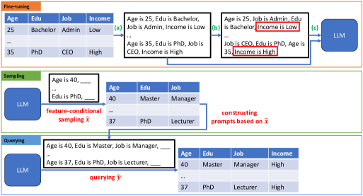
We propose a LLM-based method (called Pred-LLM) to generate a synthetic dataset that mimics the real dataset and captures the correlation between and accurately. As shown in Figure 3, our method has three phases: (1) fine-tuning a pre-trained LLM with tabular data, (2) generating samples conditioned on each feature , and (3) constructing prompts based on to query labels .
III-B1 Fine-tuning
In the first phase fine-tuning (top plot), we have three steps: (a) textual encoding, (b) permutation, and (c) fine-tuning a pre-trained LLM.
(a) Textual encoding. As our method uses LLM to generate tabular data, following other works [7, 48] we convert each sample and its label into a sentence. Although there are several methods to serialize a tabular row [16], we use a simple strategy that transforms the th row into a corresponding sentence , where are feature names, is the value of the th feature of the th sample, is the target variable and is its value. For example, the first row is converted into “Age is 25, Edu is Bachelor, Job is Admin, Income is Low”.
(b) Permutation. Recall that existing LLM-based methods permute both the features and the target variable . We call this strategy permute_xy. Formally, given a sentence , we re-write it in a short form , where with , , and denotes the concatenation operator. The permutation strategy permute_xy applies a permutation function to randomly shuffle the order of the features and the target variable. This step results in a permuted sentence , where . For example, the sentence “Age is 25, Edu is Bachelor, Job is Admin, Income is Low” is permuted to “Income is Low, Edu is Bachelor, Job is Admin, Age is 25”.
In contrast, we only permute the features while fixing the target variable at the end. We call our strategy permute_x. Formally, given a sentence , we apply the permutation function to features only, which results in a permuted sentence , where . For example, the sentence “Age is 25, Edu is Bachelor, Job is Admin, Income is Low” is permuted to “Age is 25, Job is Admin, Edu is Bachelor, Income is Low”. Note that the target variable “Income” and its value “Low” are at the end of the permuted sentence.
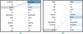
Our permutation strategy ensures that our LLM can learn the attention links from the features to the target variable , which helps to capture the correlation between and . In Figure 4, we use BertViz [42] to visualize the attention links learned by ChatGPT-2 – the LLM model used in LLM-based methods such as Great [7], TapTap [48], and our Pred-LLM. As Great and TapTap use the permutation strategy permute_xy, there is no attention link between the label “Low” with other features when the target variable “Income” is shuffled to the beginning of the sentence, as shown in (a). As our method uses the permutation strategy permute_x, our attention matrix can capture some strong correlations between the label “Low” and the features “Age” and “Edu”, as shown in (b).
(c) Fine-tuning. While other LLM-based methods use the permute_xy version of the dataset to fine-tune the LLM, we fine-tune our LLM with the dataset permuted with our strategy permute_x. As we also want to keep the original order of the features, we augment the permuted data with the original data when fine-tuning the model, as shown in step (c). This step is necessary because in a later step where we construct a prompt based on a generated sample to query its label , we follow the original order of the features in the real dataset.
We fine-tune our LLM following an auto-regressive manner i.e. we train it to predict the next token given a set of observed tokens in each encoded sentence. Given a textually encoded tabular dataset , for each sentence , we tokenize it into a sequence of tokens , where are required tokens to describe the sentence . Following an auto-regressive manner, we factorize the probability of a sentence into a product of output probabilities conditioned on previously observed tokens:
| (1) |
III-B2 Sampling
In the second phase sampling (middle plot), we generate synthetic samples . Given an input sequence of tokens , our fine-tuned LLM returns logits over all possible follow-up tokens:
The next token is sampled from a conditional probability distribution defined by a softmax function that is modified by a temperature to soften the output distribution:
| (2) |
where is an exponential function and is the complete set of all unique tokens i.e. the vocabulary.
To generate , we need to initialize the sequence of tokens and use it as a condition for the sampling step. As we employ permutation during the fine-tuning phase, our method also supports arbitrary conditioning like other LLM-based methods. In other words, we can use any set of features as a condition. As mentioned in the literature, there are several ways to create a condition. The most popular way is to use a pair of the target variable and its value as a condition [7, 48]. In particular, a label is first sampled from the distribution of the target variable i.e. . The condition is then constructed as “” e.g. “Income is Low”. We call this strategy class-conditional sampling.
In contrast, our method follows a feature-conditional sampling style. We first uniformly sample a feature from the list of features . We then sample a value from the distribution of i.e. . Finally, we construct our condition as “” e.g. “Age is 40”.
Our sampling strategy has an advantage. As we generate the features before the target variable , our LLM can use all learned attention links from to to generate more accurately. However, it also has a weakness. As we cannot control when is generated, the correlations between and some features may be missed. For example, assume that we use as a condition. From , using Equation (2), we may generate . Conditioned on , we may generate . In this case, we generate with only attentions coming from two features and , and we may miss the attentions from the other features. We address this problem in the next step.
III-B3 Querying
In the final phase querying (last plot), we construct prompts to query our LLM for labels. After generating a synthetic sample with all features, we construct a prompt based on as “” and use it as a condition to sampling . Using this way, our LLM can utilize the learned attention links from all features to better generate the target variable . Moreover, our LLM behaves like a predictive model, and we generate from a conditional distribution . This strategy works very well thanks to the accurate correlation between and captured by our LLM.
III-B4 Algorithm
Algorithm 1 presents the pseudo-code of our method Pred-LLM. It has three phases: fine-tuning, sampling, and querying. In the fine-tuning phase (lines 4-8), we textually encode each row to a sentence, permute it using our permutation strategy permute_x, and create a new dataset that contains permuted sentences and original sentences (line 7). Finally, we use to fine-tune a pre-trained LLM .
In the sampling phase (lines 17-22), we generate synthetic samples using our feature-conditional sampling approach. For each feature , we use it as a condition to sample data from our fine-tuned LLM . Note that the number of synthetic samples conditioned on each is sampled equally (line 16).
In the querying phase (lines 24-27), we construct prompts based on generated samples to query their labels . In this case, we use our LLM as a predictive model to generate labels.
IV Experiments
We conduct extensive experiments to show that our method is much better than other methods under different qualitative and quantitative metrics.
IV-A Experiment settings
IV-A1 Datasets
We evaluate our method on 20 real-world tabular datasets. They are commonly used in predictive and generation tasks [44, 28, 21, 7, 48]. The details of these datasets are provided in Table I.
| Dataset | Source | |||
|---|---|---|---|---|
| iris | 150 | 4 | 3 | scikit-learn |
| breast_cancer (breast) | 569 | 30 | 2 | scikit-learn |
| blood_transfusion (blood) | 748 | 4 | 2 | OpenML |
| steel_plates_fault (steel) | 1,941 | 33 | 2 | OpenML |
| diabetes | 768 | 8 | 2 | OpenML |
| australian | 690 | 14 | 2 | OpenML |
| balance_scale (balance) | 625 | 4 | 3 | OpenML |
| compas | 4,010 | 10 | 2 | [29] |
| bank | 4,521 | 14 | 2 | [29] |
| adult | 30,162 | 13 | 2 | UCI |
| qsar_biodeg (qsar) | 1,055 | 41 | 2 | OpenML |
| phoneme | 5,404 | 5 | 2 | OpenML |
| waveform | 5,000 | 40 | 3 | OpenML |
| churn | 5,000 | 20 | 2 | OpenML |
| kc1 | 2,109 | 21 | 2 | OpenML |
| kc2 | 522 | 21 | 2 | OpenML |
| cardiotocography (cardio) | 2,126 | 35 | 10 | OpenML |
| abalone | 4,177 | 8 | regression | Kaggle |
| fuel | 639 | 8 | regression | Kaggle |
| california | 20,640 | 8 | regression | scikit-learn |
IV-A2 Evaluation metric
To evaluate the performance of tabular generation methods, we use the synthetic data in predictive tasks (Figure 1) similar to other works [44, 21, 7]. For each dataset, we randomly split it into 80% for the real set and 20% for the test set . We train tabular generation methods on to generate the synthetic set , where . Finally, we train XGBoost on and compute its accuracy/MSE on . We repeat each method three times with random seeds and report the average score along with its standard deviation.
We also compute other metrics between and to measure the quality and diversity of the synthetic samples:
(1) Discriminator score [7]: We train a XGBoost discriminator to differentiate the synthetic data from the real data. The score of means two datasets are indistinguishable whereas means two datasets are totally distinguishable (i.e. synthetic samples are easily detectable). A lower score is better.
(2) Inverse Kullback–Leibler divergence [32]: We compute the inverse of the Kullback-Leibler averaged over all features to measure how the distribution of the synthetic data is different from the distribution of the real data . Let be a feature (i.e. a column) in the real table and be its corresponding feature in the synthetic table , the inverse KL score between and is . As , is finite, which results in . The score of means two datasets are from different distributions whereas means they are from the same distribution. A higher score is better.
(3) Density [26]: We compute the density score , where is the sphere around with the radius being the Euclidean distance from to its -th nearest neighbor (we set ). It measures how many synthetic samples reside in the neighbor of the real samples . It measures the quality of the synthetic samples as it shows how the synthetic samples are similar/close to the real samples. A higher score is better.
(4) Coverage [26]: We compute the coverage score . It measures the fraction of real samples whose neighborhoods contain at least one synthetic sample . It measures the diversity of the synthetic samples as it shows how the synthetic samples resemble the variability of the real samples. A higher score is better.
IV-A3 Baselines
We compare with 10 SOTA baselines. They include GAN-based methods (CopulaGAN [31], MedGAN [10], VeeGAN [37], TableGAN [30], CTGAN [44], TabGAN [3], and OCTGAN [21]), VAE-based method (TVAE [44]), and LLM-based methods (Great [7] and TapTap [48]).
The Original method means the predictive model trained with the real dataset . We use XGBoost for the predictive model since it is one of the most popular models for tabular data [36]. Following [7, 48], we use the distilled version of ChatGPT-2 for our LLM, and train it with batch_size=32 and #epochs=50. We set for Equation (2).
IV-B Results and discussions
IV-B1 Downstream predictive tasks
Table II reports accuracy and MSE of each method on 20 benchmark datasets. We recall that the procedure to compute the scores is described in Figure 1. Our method Pred-LLM performs better than other methods. Among 20 datasets, Pred-LLM is the best performing on nine datasets and the second-best on another nine datasets.
| Accuracy | Original | Copula* | Med* | Vee* | Table* | CT* | Tab* | OCT* | TVAE | Great | TapTap | Pred-LLM |
|---|---|---|---|---|---|---|---|---|---|---|---|---|
| iris | 0.9555 | 0.3445 | 0.0000 | 0.0000 | 0.0000 | 0.4444 | 0.2667 | 0.7222 | 0.9000 | 0.3667 | 0.8778 | 0.9889 |
| (0.031) | (0.057) | (0.000) | (0.000) | (0.000) | (0.150) | (0.072) | (0.103) | 0.055) | (0.098) | (0.069) | (0.016) | |
| breast | 0.9708 | 0.5409 | 0.4445 | 0.5439 | 0.0000 | 0.4796 | 0.3889 | 0.6667 | 0.9123 | 0.5760 | 0.8889 | 0.9503 |
| (0.004) | (0.062) | (0.132) | (0.124) | (0.000) | (0.092) | (0.039) | (0.186) | (0.031) | (0.097) | (0.017) | (0.015) | |
| blood | 0.7444 | 0.7178 | 0.5733 | 0.5733 | 0.6667 | 0.7355 | 0.7645 | 0.6022 | 0.7445 | 0.6866 | 0.7422 | 0.7489 |
| (0.022) | (0.014) | (0.245) | (0.236) | (0.043) | (0.030) | (0.003) | (0.073) | (0.019) | (0.041) | (0.006) | (0.025) | |
| steel | 1.0000 | 0.5955 | 0.4139 | 0.4559 | 0.9280 | 0.6298 | 0.6564 | 0.6573 | 0.6829 | 0.6392 | 0.9135 | 1.0000 |
| (0.000) | (0.035) | (0.095) | (0.101) | (0.015) | (0.027) | (0.003) | (0.006) | (0.001) | (0.045) | (0.018) | (0.000) | |
| diabetes | 0.7598 | 0.4827 | 0.5195 | 0.5325 | 0.6494 | 0.5909 | 0.6147 | 0.5757 | 0.7035 | 0.6039 | 0.7662 | 0.7099 |
| (0.037) | (0.046) | (0.102) | (0.090) | (0.058) | (0.060) | (0.021) | (0.089) | (0.030) | (0.014) | (0.024) | (0.045) | |
| australian | 0.8768 | 0.4299 | 0.5797 | 0.4541 | 0.8092 | 0.5459 | 0.5387 | 0.6015 | 0.7753 | 0.6836 | 0.8865 | 0.8768 |
| (0.006) | (0.015) | (0.095) | (0.028) | (0.036) | (0.106) | (0.018) | (0.048) | (0.033) | (0.036) | (0.017) | (0.026) | |
| balance | 0.8613 | 0.4773 | 0.0000 | 0.1627 | 0.4373 | 0.4640 | 0.3947 | 0.4453 | 0.0000 | 0.4693 | 0.8613 | 0.8507 |
| (0.010) | (0.032) | (0.000) | (0.056) | (0.061) | (0.013) | (0.051) | (0.133) | (0.000) | (0.025) | (0.014) | (0.036) | |
| compas | 0.8317 | 0.8134 | 0.5208 | 0.5964 | 0.5719 | 0.8284 | 0.8379 | 0.6563 | 0.8209 | 0.8188 | 0.8313 | 0.8317 |
| (0.003) | (0.028) | (0.256) | (0.123) | (0.082) | (0.007) | (0.000) | (0.204) | (0.030) | (0.003) | (0.007) | (0.004) | |
| bank | 0.8803 | 0.8656 | 0.6659 | 0.6302 | 0.7319 | 0.8556 | 0.8604 | 0.5901 | 0.8641 | 0.8685 | 0.8840 | 0.8847 |
| (0.007) | (0.025) | (0.155) | (0.258) | (0.126) | (0.028) | (0.015) | (0.417) | (0.008) | (0.003) | (0.002) | (0.002) | |
| adult | 0.8624 | 0.8284 | 0.5788 | 0.4367 | 0.7559 | 0.8261 | 0.7239 | 0.2498 | 0.8253 | 0.8460 | 0.8528 | 0.8530 |
| (0.000) | (0.008) | (0.231) | (0.081) | (0.019) | (0.004) | (0.020) | (0.353) | (0.005) | (0.002) | (0.003) | (0.001) | |
| qsar | 0.8752 | 0.6477 | 0.3412 | 0.4771 | 0.6983 | 0.6493 | 0.6319 | 0.5972 | 0.7899 | 0.5008 | 0.6619 | 0.7946 |
| (0.012) | (0.020) | (0.008) | (0.132) | (0.041) | (0.026) | (0.038) | (0.071) | (0.020) | (0.037) | (0.023) | (0.024) | |
| phoneme | 0.8970 | 0.7018 | 0.5134 | 0.4983 | 0.7321 | 0.7333 | 0.6876 | 0.5183 | 0.7684 | 0.7700 | 0.8705 | 0.8541 |
| (0.006) | (0.006) | (0.111) | (0.061) | (0.021) | (0.028) | (0.029) | (0.164) | (0.009) | (0.025) | (0.001) | (0.007) | |
| waveform | 0.8467 | 0.3817 | 0.0000 | 0.3297 | 0.8330 | 0.3867 | 0.3457 | 0.1147 | 0.8350 | 0.3557 | 0.7473 | 0.8473 |
| (0.004) | (0.028) | (0.000) | (0.002) | (0.002) | (0.032) | (0.014) | (0.162) | (0.005) | (0.023) | (0.020) | (0.005) | |
| churn | 0.9580 | 0.8450 | 0.6390 | 0.3987 | 0.8653 | 0.8423 | 0.8467 | 0.2793 | 0.8547 | 0.8333 | 0.9090 | 0.8703 |
| (0.002) | (0.012) | (0.047) | (0.308) | (0.003) | (0.012) | (0.002) | (0.301) | (0.021) | (0.006) | (0.006) | (0.017) | |
| kc1 | 0.8547 | 0.7986 | 0.8468 | 0.6153 | 0.7093 | 0.7986 | 0.8460 | 0.5561 | 0.8444 | 0.8160 | 0.8144 | 0.8389 |
| (0.006) | (0.036) | (0.006) | (0.325) | (0.034) | (0.041) | (0.000) | (0.393) | (0.002) | (0.013) | (0.006) | (0.005) | |
| kc2 | 0.8127 | 0.7619 | 0.4032 | 0.4095 | 0.0000 | 0.7714 | 0.7937 | 0.6540 | 0.8572 | 0.7841 | 0.8254 | 0.8190 |
| (0.022) | (0.028) | (0.281) | (0.283) | (0.000) | (0.016) | (0.005) | (0.133) | (0.014) | (0.020) | (0.025) | (0.008) | |
| cardio | 1.0000 | 0.2222 | 0.0000 | 0.0000 | 0.6229 | 0.2387 | 0.0000 | 0.0000 | 0.8052 | 0.1988 | 0.8998 | 1.0000 |
| (0.000) | (0.027) | (0.000) | (0.000) | (0.102) | (0.050) | (0.000) | (0.000) | (0.028) | (0.036) | (0.025) | (0.000) | |
| Average | 0.8816 | 0.6150 | 0.4141 | 0.4185 | 0.5889 | 0.6365 | 0.5999 | 0.4992 | 0.7637 | 0.6363 | 0.8372 | 0.8658 |
| MSE | Original | Copula* | Med* | Vee* | Table* | CT* | Tab* | OCT* | TVAE | Great | TapTap | Pred-LLM |
| abalone | 5.2213 | 8.1660 | 43.6048 | 24.3119 | 6.1970 | 8.3744 | 40.1766 | 16.6444 | 7.4558 | 11.1428 | 5.4765 | 5.6194 |
| (0.305) | (0.576) | (11.052) | (3.997) | (0.056) | (0.403) | (15.986) | (2.962) | (0.405) | (1.154) | (0.382) | (0.470) | |
| fuel | 0.0760 | 15.9164 | 19.2074 | 26.2352 | 1.5805 | 22.5587 | 17.7842 | 20.7891 | 4.6480 | 15.9838 | 0.2237 | 0.8260 |
| (0.019) | (4.579) | (6.303) | (5.552) | (0.685) | (7.015) | (6.258) | (11.297) | (1.756) | (3.776) | (0.118) | (0.360) | |
| california | 0.2696 | 0.7531 | 2.3306 | 2.8342 | 0.8680 | 0.7208 | 1.8239 | 1.4400 | 0.6248 | 0.3556 | 0.3286 | 0.3058 |
| (0.008) | (0.043) | (0.156) | (1.045) | (0.044) | (0.064) | (0.279) | (0.130) | (0.026) | (0.011) | (0.006) | (0.008) | |
| Average | 1.8556 | 8.2785 | 21.7143 | 17.7938 | 2.8818 | 10.5513 | 19.9282 | 12.9578 | 4.2429 | 9.1607 | 2.0096 | 2.2504 |
For classification tasks, the average improvement of Pred-LLM over TapTap (the runner-up baseline) is . CTGAN is the best GAN-based method, followed by CopulaGAN. Other GAN-based baselines do not perform as well. The LLM-based method Great is comparable with CTGAN. TVAE often outperforms GAN-based methods since it has a reconstruction loss to guarantee that the synthetic samples are similar to the real samples. The same observation was also made in [44]. For regression tasks, Pred-LLM and TapTap perform comparably.
IV-B2 Quality and diversity evaluation
As described in Section IV-A2, we compute four metrics. Discriminator and Density scores measure the quality of synthetic samples, Inverse KL score measures the quality of the synthetic distribution, and Coverage score measures the diversity of synthetic samples.
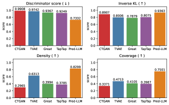
Figure 5 presents the average scores on top-5 methods on all datasets. Our method Pred-LLM significantly outperforms other methods for all metrics. The Discriminator scores show the baseline synthetic samples are easily detected by the discriminator ( chance) whereas only of our synthetic samples are detectable. Another quality metric Density shows our synthetic samples are much closer to the real samples than other synthetic samples (e.g. of Pred-LLM vs. of TVAE). The Inverse KL shows our synthetic samples and the real samples come from a similar distribution. In terms of diversity, our synthetic samples are much more diverse than others (e.g. of Pred-LLM vs. of TVAE).
High scores in both quality and diversity metrics show our synthetic samples can capture the real data manifold, which explains their benefits in downstream tasks (see Table II).
IV-C Ablation studies
We analyze our method under different configurations.
IV-C1 Effect investigation of various modifications
We have three novel contributions in permutation, sampling, and label-querying steps. Table III reports the accuracy for each modification compared to two LLM baselines Great and TapTap. Recall that the baselines permute the features and the target variable (denoted by permute_xy), and they use as a sampling condition (denoted by target_variable). Great generates both and simultaneously (denoted by querying =none) whereas TapTap generates first and then uses an external classifier to predict (denoted by querying =classifier).
While Great only achieves , our modifications show improvements. By using each feature as a sampling condition (denoted by each_feature) or prompting the LLM model for (denoted by querying =LLM), we achieve up to ( improvement). Combining these two proposals with fine-tuning our LLM on the dataset permuted by our permutation strategy (denoted by permute_x), we achieve the best result at 0.8658 (last row). This study suggests that each modification is useful, which greatly improves Great and TapTap.
| Permutation | Sampling | Querying | Accuracy | |
|---|---|---|---|---|
| Great | permute_xy | target_variable | none | 0.6363 |
| TapTap | permute_xy | target_variable | classifier | 0.8372 |
| Pred-LLM | permute_x | target_variable | none | 0.6191 |
| permute_xy | each_feature | none | 0.7352 | |
| permute_xy | target_variable | LLM | 0.7307 | |
| permute_xy | each_feature | LLM | 0.7477 | |
| permute_x | target_variable | LLM | 0.8495 | |
| permute_x | each_feature | LLM | 0.8658 |
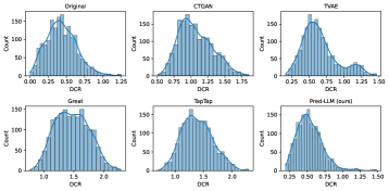
IV-C2 Distance to closest records (DCR) histogram
Following [7], we plot the DCR histogram to show our synthetic dataset is similar to the real dataset but it is not simply duplicated. The DCR metric computes the distance from a real sample to its closest neighbor in the synthetic dataset. Given a real sample , . We use the Euclidean distance for the distance function .
Figure 6 visualizes the DCR distributions of top-5 methods. Only our method Pred-LLM and TVAE can generate synthetic samples in close proximity to the real samples. Other methods show significant differences.
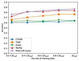
IV-C3 Effect investigation of training size and generation size
We investigate the effect of the numbers of real and synthetic samples on the performance of our method. Recall that we use as the training data to train tabular generation methods and generate the same number of synthetic samples as the number of real samples (i.e. ).
Figure 7(a) shows our method Pred-LLM improves when the training size increases. It is improved significantly when trained with the full original training set, improving from 0.7610 to 0.8658. The baseline TapTap also benefits with more real training samples, improving from 0.7229 to 0.8372. However, there remains a big gap between its performance and ours. Similar trends are also observed for other methods.
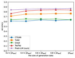
Figure 7(b) shows the accuracy when we train the predictive model XGBoost with different numbers of synthetic samples . Here, we still use the full real dataset to train tabular generation methods to generate different cases of . The classifier is better when it is trained with more synthetic samples produced by tabular generation methods except Great. When generating more synthetic samples, Great causes the classifier’s accuracy slightly reduced from 0.6523 down to 0.6363. Our method Pred-LLM makes the classifier better when it is trained with larger generated data, where the accuracy improves from 0.8395 to 0.8658.
IV-C4 Weakness of TapTap
After generating a synthetic sample , TapTap uses a classifier trained on the real dataset (i.e. the Original method) to predict , which works well in most cases. However, when TapTap generates the synthetic samples whose distribution is not similar to that of the real samples, the classifier may wrongly predict the labels. As shown in Table IV, the Original method has high accuracy on the real test set as . However, as TapTap cannot generate in-distribution samples i.e. (indicated by its low Inverse KL scores), the Original method wrongly predicts for , leading to a significant downgrade in TapTap’s performance.
| Original | TapTap | ||
|---|---|---|---|
| Accuracy | Inverse KL | Accuracy | |
| breast | 0.9708 | 0.5652 | 0.8889 |
| steel | 1.0000 | 0.6208 | 0.9135 |
| qsar | 0.8752 | 0.5839 | 0.6619 |
| waveform | 0.8467 | 0.4815 | 0.7473 |
| cardio | 1.0000 | 0.7205 | 0.8998 |
IV-D Visualization
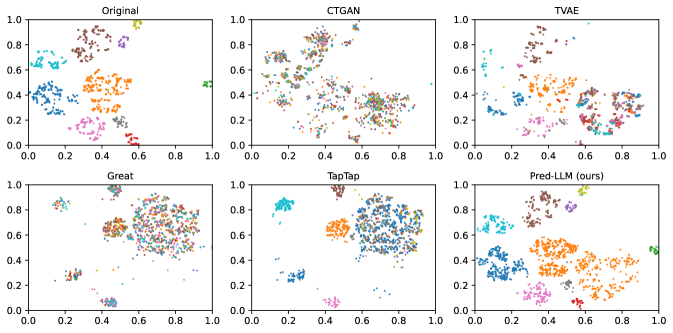
For a quantitative evaluation, we use t-SNE [41] to visualize the synthetic samples and compare them with the real samples.
Figure 8 shows synthetic samples along with their labels. Here, each color indicates each class. From the real data (the 1st plot), we can see the “green” samples lie in the middle of the right region while the other samples lie in the left region. Our method Pred-LLM (the last plot) is the only method that can capture this class distribution and generate synthetic samples close to the real samples. In contrast, other methods generate out-of-distribution synthetic samples, and they cannot capture the true class distribution of the real samples.
V Conclusion
In this paper, we address the problem of synthesizing tabular data by developing a LLM-based method (called Pred-LLM). Different from existing methods, we propose three important contributions in fine-tuning, sampling, and querying phases. First, we propose a novel permutation strategy during the fine-tuning of a pre-trained LLM, which helps to capture the correlation between the features and the target variable. Second, we propose the feature-conditional sampling to generate synthetic samples, where each feature can be conditioned on iteratively. Finally, instead of leveraging an external classifier to predict the labels for the generated samples, we construct the prompts based on the generated data to query the labels. Our method offers significant improvements over 10 SOTA baselines on 20 real-world datasets in terms of downstream predictive tasks, and the quality and the diversity of synthetic samples. By generating more synthetic samples, our method can help other applications such as few-shot knowledge distillation [27] and algorithmic assurance [14] with few samples.
Acknowledgment: This research was partially supported by the Australian Government through the Australian Research Council’s Discovery Projects funding scheme (project DP210102798). The views expressed herein are those of the authors and are not necessarily those of the Australian Government or Australian Research Council.
References
- [1] Ewa Andrejczuk, Julian Eisenschlos, Francesco Piccinno, Syrine Krichene, and Yasemin Altun. Table-To-Text generation and pre-training with TabT5. In EMNLP, pages 6758–6766, 2022.
- [2] Martin Arjovsky, Soumith Chintala, and Léon Bottou. Wasserstein Generative Adversarial Networks. In ICML, pages 214–223, 2017.
- [3] Insaf Ashrapov. Tabular GANs for uneven distribution. arXiv preprint arXiv:2010.00638, 2020.
- [4] Junwei Bao, Duyu Tang, Nan Duan, Zhao Yan, Yuanhua Lv, Ming Zhou, and Tiejun Zhao. Table-to-text: Describing table region with natural language. In AAAI, volume 32, 2018.
- [5] Iz Beltagy, Kyle Lo, and Arman Cohan. SciBERT: A Pretrained Language Model for Scientific Text. In EMNLP-IJCNLP, pages 3615–3620, 2019.
- [6] Vadim Borisov, Tobias Leemann, Kathrin Seßler, Johannes Haug, Martin Pawelczyk, and Gjergji Kasneci. Deep neural networks and tabular data: A survey. IEEE Transactions on Neural Networks and Learning Systems, 2022.
- [7] Vadim Borisov, Kathrin Seßler, Tobias Leemann, Martin Pawelczyk, and Gjergji Kasneci. Language models are realistic tabular data generators. In ICLR, 2023.
- [8] Tianqi Chen and Carlos Guestrin. Xgboost: A scalable tree boosting system. In KDD, pages 785–794, 2016.
- [9] Wenhu Chen, Hongmin Wang, Jianshu Chen, Yunkai Zhang, Hong Wang, Shiyang Li, Xiyou Zhou, and Yang Wang. TabFact : A Large-scale Dataset for Table-based Fact Verification. In ICLR, 2020.
- [10] Edward Choi, Siddharth Biswal, Bradley Malin, Jon Duke, Walter Stewart, and Jimeng Sun. Generating multi-label discrete patient records using generative adversarial networks. In Machine Learning for Healthcare Conference, pages 286–305. PMLR, 2017.
- [11] Zihang Dai, Zhilin Yang, Yiming Yang, Jaime Carbonell, Quoc Le, and Ruslan Salakhutdinov. Transformer-XL: Attentive language models beyond a fixed-length context. arXiv preprint arXiv:1901.02860, 2019.
- [12] Cristóbal Esteban, Stephanie Hyland, and Gunnar Rätsch. Real-valued (medical) time series generation with Recurrent Conditional GANs. arXiv preprint arXiv:1706.02633, 2017.
- [13] Ian Goodfellow, Jean Pouget-Abadie, Mehdi Mirza, Bing Xu, David Warde-Farley, Sherjil Ozair, Aaron Courville, and Yoshua Bengio. Generative Adversarial Nets. In NeurIPS, volume 27, 2014.
- [14] Shivapratap Gopakumar, Sunil Gupta, Santu Rana, Vu Nguyen, and Svetha Venkatesh. Algorithmic Assurance: An Active Approach to Algorithmic Testing using Bayesian Optimisation. In NeurIPS, pages 5466–5474, 2018.
- [15] Manbir Gulati and Paul Roysdon. TabMT: Generating tabular data with masked transformers. NeurIPS, 36, 2024.
- [16] Stefan Hegselmann, Alejandro Buendia, Hunter Lang, Monica Agrawal, Xiaoyi Jiang, and David Sontag. Tabllm: Few-shot classification of tabular data with large language models. In AISTAT, pages 5549–5581, 2023.
- [17] Jonathan Herzig, Pawel Krzysztof Nowak, Thomas Müller, Francesco Piccinno, and Julian Eisenschlos. TaPas: Weakly Supervised Table Parsing via Pre-training. In ACL, pages 4320–4333, 2020.
- [18] Martin Heusel, Hubert Ramsauer, Thomas Unterthiner, Bernhard Nessler, and Sepp Hochreiter. Gans trained by a two time-scale update rule converge to a local nash equilibrium. NeurIPS, 30, 2017.
- [19] James Jordon, Jinsung Yoon, and Mihaela Van Der Schaar. PATE-GAN: Generating synthetic data with differential privacy guarantees. In ICLR, 2019.
- [20] Guolin Ke, Qi Meng, Thomas Finley, Taifeng Wang, Wei Chen, Weidong Ma, Qiwei Ye, and Tie-Yan Liu. Lightgbm: A highly efficient gradient boosting decision tree. In NeurIPS, volume 30, 2017.
- [21] Jayoung Kim, Jinsung Jeon, Jaehoon Lee, Jihyeon Hyeong, and Noseong Park. Oct-GAN: Neural ode-based conditional tabular gans. In Proceedings of the Web Conference, pages 1506–1515, 2021.
- [22] Diederik Kingma, Max Welling, et al. An introduction to variational autoencoders. Foundations and Trends in Machine Learning, 12(4):307–392, 2019.
- [23] Nikita Kitaev, Łukasz Kaiser, and Anselm Levskaya. Reformer: The efficient transformer. arXiv preprint arXiv:2001.04451, 2020.
- [24] Scott Lundberg and Su-In Lee. A unified approach to interpreting model predictions. In NeurIPS, volume 30, 2017.
- [25] Jaeuk Moon, Seungwon Jung, Sungwoo Park, and Eenjun Hwang. Conditional tabular GAN-based two-stage data generation scheme for short-term load forecasting. IEEE Access, 8:205327–205339, 2020.
- [26] Muhammad Ferjad Naeem, Seong Joon Oh, Youngjung Uh, Yunjey Choi, and Jaejun Yoo. Reliable fidelity and diversity metrics for generative models. In ICML, pages 7176–7185, 2020.
- [27] Dang Nguyen, Sunil Gupta, Kien Do, and Svetha Venkatesh. Black-box few-shot knowledge distillation. In ECCV, pages 196–211, 2022.
- [28] Dang Nguyen, Sunil Gupta, Santu Rana, Alistair Shilton, and Svetha Venkatesh. Bayesian optimization for categorical and category-specific continuous inputs. In AAAI, volume 34, pages 5256–5263, 2020.
- [29] Dang Nguyen, Sunil Gupta, Santu Rana, Alistair Shilton, and Svetha Venkatesh. Fairness Improvement for Black-box Classifiers with Gaussian Process. Information Sciences, 576:542–556, 2021.
- [30] Noseong Park, Mahmoud Mohammadi, Kshitij Gorde, Sushil Jajodia, Hongkyu Park, and Youngmin Kim. Data Synthesis Based on Generative Adversarial Networks. Proceedings of the VLDB Endowment, 11(10):1071–1083, 2018.
- [31] Neha Patki, Roy Wedge, and Kalyan Veeramachaneni. The synthetic data vault. In International Conference on Data Science and Advanced Analytics (DSAA), pages 399–410, 2016.
- [32] Zhaozhi Qian, Bogdan-Constantin Cebere, and Mihaela van der Schaar. Synthcity: facilitating innovative use cases of synthetic data in different data modalities. arXiv preprint arXiv:2301.07573, 2023.
- [33] Alec Radford, Karthik Narasimhan, Tim Salimans, Ilya Sutskever, et al. Improving language understanding by generative pre-training. 2018.
- [34] Amirarsalan Rajabi and Ozlem Ozmen Garibay. TabFairGAN: Fair tabular data generation with generative adversarial networks. Machine Learning and Knowledge Extraction, 4(2):488–501, 2022.
- [35] Nabeel Seedat, Nicolas Huynh, Boris van Breugel, and Mihaela van der Schaar. Curated LLM: Synergy of LLMs and Data Curation for tabular augmentation in ultra low-data regimes. In ICML, 2024.
- [36] Ravid Shwartz-Ziv and Amitai Armon. Tabular data: Deep learning is not all you need. Information Fusion, 81:84–90, 2022.
- [37] Akash Srivastava, Lazar Valkov, Chris Russell, Michael Gutmann, and Charles Sutton. VeeGAN: Reducing mode collapse in gans using implicit variational learning. In NeurIPS, volume 30, pages 3310–3320, 2017.
- [38] Yuan Sui, Mengyu Zhou, Mingjie Zhou, Shi Han, and Dongmei Zhang. Table meets LLM: Can large language models understand structured table data? a benchmark and empirical study. In International Conference on Web Search and Data Mining, pages 645–654, 2024.
- [39] Nan Tang, Ju Fan, Fangyi Li, Jianhong Tu, Xiaoyong Du, Guoliang Li, Sam Madden, and Mourad Ouzzani. RPT: relational pre-trained transformer is almost all you need towards democratizing data preparation. VLDB Endowment, 14(8):1254–1261, 2021.
- [40] Amirsina Torfi, Edward Fox, and Chandan Reddy. Differentially private synthetic medical data generation using Convolutional GANs. Information Sciences, 586:485–500, 2022.
- [41] Laurens Van der Maaten and Geoffrey Hinton. Visualizing data using t-SNE. Journal of Machine Learning Research, 9(11):2579–2605, 2008.
- [42] Jesse Vig. A Multiscale Visualization of Attention in the Transformer Model. In ACL, pages 37–42, 2019.
- [43] Hajra Waheed, Muhammad Anas, Saeed-Ul Hassan, Naif Radi Aljohani, Salem Alelyani, Ernest Edem Edifor, and Raheel Nawaz. Balancing sequential data to predict students at-risk using adversarial networks. Computers & Electrical Engineering, 93:107274, 2021.
- [44] Lei Xu, Maria Skoularidou, Alfredo Cuesta-Infante, and Kalyan Veeramachaneni. Modeling tabular data using Conditional GAN. In NeurIPS, volume 32, pages 7335–7345, 2019.
- [45] June Yong Yang, Geondo Park, Joowon Kim, Hyeongwon Jang, and Eunho Yang. Language-interfaced tabular oversampling via progressive imputation and self-authentication. In ICLR, 2024.
- [46] Pengcheng Yin, Graham Neubig, Wen-tau Yih, and Sebastian Riedel. TaBERT: Pretraining for Joint Understanding of Textual and Tabular Data. In ACL, pages 8413–8426, 2020.
- [47] Hongzhi Zhang, Yingyao Wang, Sirui Wang, Xuezhi Cao, Fuzheng Zhang, and Zhongyuan Wang. Table fact verification with structure-aware transformer. In EMNLP, pages 1624–1629, 2020.
- [48] Tianping Zhang, Shaowen Wang, Shuicheng Yan, Jian Li, and Qian Liu. Generative table pre-training empowers models for tabular prediction. In EMNLP, pages 14836–14854, 2023.