The evolution of two-point correlation function of galaxies with a twin-peak initial power spectrum
Abstract
The evolution equation of two-point correlation function of galaxies can analytically describe the large scale structure of the galaxy distribution, and the solution depends also upon the initial condition. The primeval spectrum of the baryon acoustic oscillations (BAO) contains multi peaks that survived the Silk damping, and, as a relevant portion, two peaks of the primeval BAO spectrum fall into the range of current galaxy surveys. Incorporating this portion, we use a twin-peak initial power spectrum of the galaxies, and obtain the evolution solution from a redshift to in the Gaussian approximation. The outcome at still exhibits the 100 Mpc periodic bumps as observed by the WiggleZ survey, a feature largely determined by the Jeans length in the equation. In particular, due to the superposition of the twin peaks in the initial condition, shows a shallow trough at Mpc and a deep trough at Mpc, agreeing with the observational data, much better than our previous work that used a simple one-peak initial spectrum.
PACS numbers:
04.40.-b Self-gravitating systems; continuous media and classical fields in curved spacetime
98.65.Dx Large-scale structure of the Universe
98.80.Jk Mathematical aspects of cosmology
1 Introduction
Progress in the observations of large-scale structure is ever increasing. Surveys for galaxies, e.g., 6dFGS [1], SDSS [4, 3, 2, 8, 5, 6, 7], WiggleZ [9], and for quasars, e.g., SDSS BOSS [11, 13, 12, 10, 14, 15], have provide rich data of the distribution of galaxies. Most of theoretical studies are numerical computations and simulations since late 70’s. Attempts on analytic study are also made in various approach [16, 17]. In particular, Davis and Peebles [18] treated the system of galaxies as a many-body system, started with the Liouville’s equation of probability function, and derived a set of BBGKY (Bogoliubov-Born-Green-Kirkwood-Yvon) equations of the two-point correlation function and of the velocity dispersions of galaxies. In particular, the equation of is not closed, and contains other unknowns. To solve these five equations, an appropriate initial condition is required for the five unknown functions, which are difficult to specify consistently. Due to these points, the BBGKY equations are hard to apply in the practical study of the large scale structure.
In our serial analytic study, using the field theoretic technique, the static equations and their solutions have been given for the two-point correlation functions [19, 20, 21, 22], for the three-point correlation functions [22, 23], and for the four-point correlation functions [24]. To describe the evolution in the expanding Universe, in Ref.[25], we derived the evolution equation of two-point correlation function in a flat Robertson-Walker spacetime, which is a closed, nonlinear, differential-integro equation. Using a simple one-peak initial power spectrum, we solved the evolution equation in the Gaussian approximation, and the solution showed the 100Mpc periodic bumps as have been observed by the early surveys [26, 27, 28, 29, 30, 31], and by more recent surveys of galaxy [9, 1, 3, 4, 2], and of quasars [10, 12, 11, 13, 14, 15]. However, the depths of the predicted two troughs at Mpc and Mpc, still deviate from the observational data. In this paper, we shall use the twin-peak initial power spectrum that inherits a relevant portion of the primeval BAO spectrum [32, 33, 34, 36, 35]. The solution will not only yield the 100Mpc periodic feature, but also predict the adequate depths of the two troughs, which agree with the observational data of the WiggleZ Survey [9].
Section 2 lists the evolution equation of in the Gaussian approximation. Section 3 presents the twin-peak initial power spectrum, and specifies the ranges of the parameters. Section 4 gives the solution and compares with the observational data. Section 5 gives the conclusion and discussion.
2 The linear equation of two-point correlation function of galaxies
The system of galaxies in the expanding Universe can be modeled by a Newtonian self-gravity fluid [38, 37], and the nonlinear field equation of the mass density is known [37]. In our previous work [25], applying the functional derivative [40, 39] to the ensemble average of the field equation of the mass density, we have derived the nonlinear equation of the two-point connected correlation function in the expanding Universe, which is a hyperbolic, differential-integro equation, and contains nonlinear terms in integrations, such as the three-point and four-point correlation functions, and , hierarchically. The nonlinear equation is complex and its solution will involve much computation. The nonlinear terms will enhance the clustering and affect the correlation function only at small scales, as the static nonlinear solution indicates [20, 21]. Dropping the nonlinear terms, the evolution equation in the Gaussian approximation is simple and valid at large scales Mpc where . In this paper we work with the evolution equation of in the Gaussian approximation [25]
| (1) |
where , is the critical density, is the mass of typical galaxy, is the overdensity parameter (), is the present sound speed of the system of galaxies, and for galaxies without or with self-rotation respectively. (See the details in Ref.[25].) The scale factor is given by with and . The normalization will be used.
The evolution equation (1) is a linear, hyperbolic equation, and holds for the system of galaxies on large scales inside the horizon of the expanding Universe. The term is due to the cosmic expansion, and has the effect of suppressing the growth of clustering. The pressure term gives rise to acoustic oscillations on the large scales, and its role is against the clustering. The gravity term is the main driving force for clustering. The inhomogeneous term is a source for the correlation function, and enhances the amplitude of correlation function [25]. Its magnitude is proportional to , and explains the observed fact that galaxies of higher mass acquire a higher correlation amplitude [41, 44, 42, 43]. In the static case , Eq.(1) will reduce to the static linear equation that was studied in Ref.[19]. By comparison, in the linear approximation of Davis-Peebles’ equation (72), the pressure term was ignored as they considered a pressureless gas, and the term was dropped in a massless limit.
The equation (1) can be solved conveniently in the -space without specifying the boundary condition. Introduce the Fourier transformation,
| (2) |
where is the power spectrum of dimension , which is related to often used in the literature. Using as the time variable, Eq.(1) leads to the ordinary differential equation of the power spectrum
| (3) |
where with being the Hubble constant,
| (4) |
is the present Jeans wavenumber, and is the present Jeans length of the system of galaxies. In the expanding Universe, the Jeans length is stretching as , slower than the comoving (). For each , Eq.(3) describes an oscillating mode when , or a growing mode when . Asides the cosmological parameters and , Eq.(3) contains , , and as the parameters of the self-gravity system of galaxies.
3 The initial condition and the parameters
An appropriate initial power spectrum of galaxies is needed to solve the differential equation (3). Currently we do not know the observed correlation function of galaxies at the early stage of formation [45]. Observations indicate that galaxies are formed not later than a redshift range [46, 47]. In our previous work [25] a simple one-peak initial power spectrum of galaxies was used at , which corresponds to the first characteristic peak of the primeval spectrum of BAO at the decoupling () [32, 33] that have survived the Silk damping [48, 49, 50]. In fact, the primeval spectrum of BAO contains multi characteristic peaks. For instance, Ref.[33] in their Figure 4 gave four BAO peaks which survive the Silk damping, for a model of baryon , with the first two peaks corresponding to the comoving wavelengths Mpc, Mpc approximately, (other two peaks corresponding to the wavelengths which are too long and beyond the range of the current galaxy surveys.) The details of these BAO peaks are model-dependent, and sensitive to the fractions of the baryon, etc. For a CDM model with , Ref.[34] gave a first peak at Mpc and a broad second peak at Mpc. (See also Refs.[36, 35] for other model parameters.) It is expected that, after the decoupling, the BAO imprints are eventually transferred to the initial power spectrum of the system of galaxies. (The detail of the transferring process is worthy of further study.) The point is that two peaks of the primeval BAO spectrum are relevant, as they fall into the range of the current galaxy surveys.
Motivated by the above analysis, we adopt a twin-peak initial power spectrum of the system of galaxies as the following
| (5) |
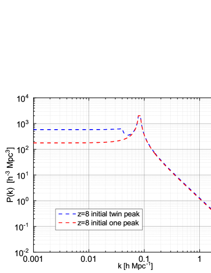
The first term in (5) is the one peak initial spectrum that was used in Ref.[25], and the second term gives a second broad peak which is newly added in this paper, is the present number density of galaxies (we take Mpc3), and are the locations of the first and second peaks, and is a step-like function to give a broad second peak, as in the primeval BAO spectrum in Refs.[34, 36, 35]. We shall choose an initial redshift for actual computing in this paper, and take and as parameters to fit with the observational data [9]. Approximately, the first peak at corresponds a comoving wavelength Mpc, and the second peak at corresponds to a comoving wavelength Mpc. The concrete expression (5) is based on the analytic static solution in Ref.[19], and has a similar profile to the initial linear spectrum used in simulations [51]. The form of the expression (5) is not unique, and other possible choices are allowed. The divergences at and in the expression (5) will be cut off in computing. Fig. 1 shows the initial twin-peak spectrum at in the blue solid line, and the red dashed line is the one peak spectrum used in Ref.[25].
To solve (3), an initial rate is also needed. The rate is defined by
| (6) |
The rate is affected by the cosmological constant [52]. For and , the initial rate at is and , respectively. Note that at , which corrects a typo in Ref.[25]. As it turns out, the outcome at low redshifts is not very sensitive to the value of initial rate.
In our computing, the cosmological parameters are taken in the range , and Mpc with . To fit with the observational data of the correlation function from the WiggleZ surveys [9], the fluid parameters can be taken in the range , i.e., , , . These ranges of parameters are similar to those used in the previous work [25].
4 The Results
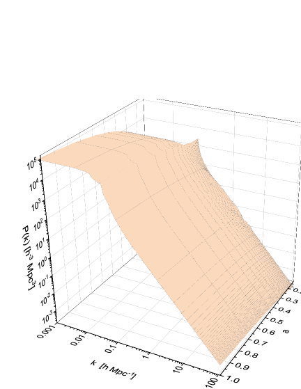
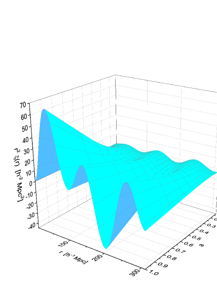
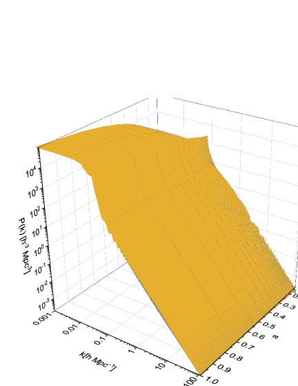
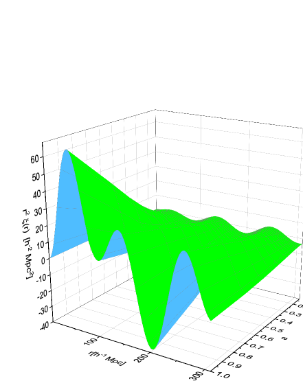
Given the equation (3), together with the twin-peak initial condition (5) (6) at , we obtain numerically the solution for each , and by Fourier transformation. The whole evolution from to of the spectrum and the weighted are shown in Fig.2 for the model , and in Fig.3 for the model , respectively. During the evolution, keeps a profile similar to the initial , and is increasing in amplitude. contains periodic bumps and troughs, the bumps are getting higher and the troughs are getting deeper, and the separation between bumps is stretching to a greater distance. The evolution is quite smooth and there are no abrupt jumps, and in this sense the distribution of galaxies is in an asymptotically relaxed state in the expanding Universe [16].
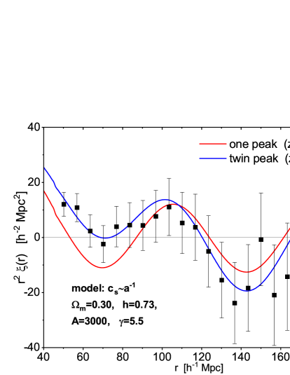
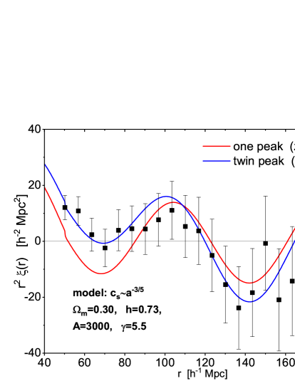
To compare with the WiggleZ data with a mean redshift [9], we plot the output at in Fig.4 for and in Fig.5 for , and the outcome by the one-peak initial spectrum [25] is also given for comparison. Prominently, the periodic bumps of the weighted occur and are located approximately at
| (7) |
the bump separation Mpc which is identified as the Jeans length in eq.(3). This periodicity occurs also in the static solution [19, 20, 21], and in the evolution solution with the one peak initial spectrum [25], and now shows up the solution with the twin-peak initial spectrum. Early pencil-beam redshift surveys already observed the 100Mpc periodic feature in the correlation function of galaxies [26, 27, 28] and of clusters [29, 30, 31]. Recent surveys observe two bumps, one at Mpc and another at Mpc, in the correlation function of galaxy [9, 1, 3, 4, 2], as well as of quasars [10, 12, 11, 13, 14]. All these observational results confirm the predicted 100Mpc periodic feature (7). Some simulations also show this phenomenon [53]. In the future there may be a chance of detecting the third bump at Mpc as our result (7) predicts. Our computing shows that the 100Mpc periodicity is also slightly modified by the initial spectrum and by other parameters as well.
An important result by using the twin-peak initial spectrum is the prediction of a shallow trough at Mpc and a deep trough at Mpc in the correlation function. This results from the superposition of the twin peaks of the initial spectrum. The second peak at corresponds to a very long wavelength Mpc, affects the profile due to the first peak, and consequently modifies the depths of the two troughs at Mpc and Mpc. The right panels of Fig.4 and Fig.5 show that the profiles of the two troughs match the data of WiggleZ [9], much better than those from the one-peak initial spectrum [25]. The outcomes from the two initial power spectra can be compared by using the chi-square as a statistical test,
| (8) |
where is the observed value, is the theoretical value, and is the variance of observed value. In the model , we get for the twin-peak initial spectrum, and for the one-peak initial spectrum, and respectively, in the model , for the twin-peak initial spectrum, and for the one-peak initial spectrum. So, statistically the twin-peak initial spectrum gives a better account of the observational data than the one-peak initial spectrum.
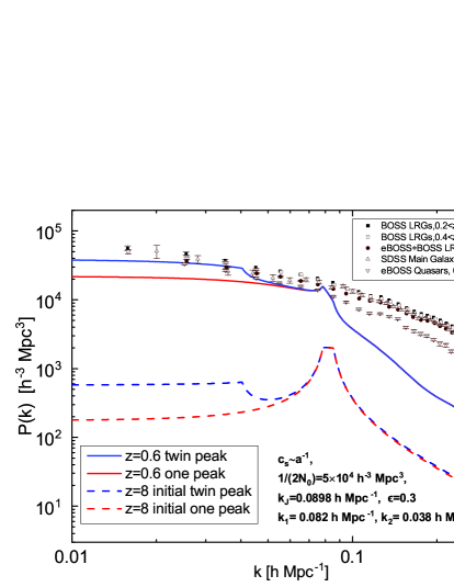
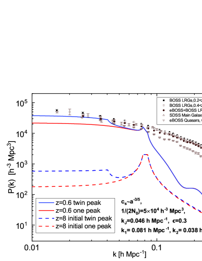
Although we have chosen the parameters to fit the observed of the WiggleZ [9], nevertheless, the associated outcome at large scales is also qualitatively consistent with the observed power spectrum of eBOSS and SDSS [8, 5, 15, 6, 7]. At small scales (Mpc-1) is lower than the data, and this is the limitation of the Gaussian approximate eq.(3) in which the nonlinear terms have not been included [25].
5 Conclusion and discussion
We study the evolution equation of the correlation function of galaxies in the Gaussian approximation, and use the twin-peak initial power spectrum (5) at , which inherits a relevant portion of the imprints of the primeval BAO spectrum [33, 34]. The evolution of the power spectrum and the two-point correlation function are obtained. not only contains the Mpc periodic bumps, but also predicts a shallow trough at Mpc and a deep trough at Mpc, agreeing with the observational data of WiggleZ [9] up to the range Mpc. The outcome improves substantially the previous work that used the simple one-peak initial spectrum [25].
The periodic bump separation Mpc is determined by the Jeans wavelength in Eq.(3), mildly modified by the first peak at (short-wavelength) of the initial power spectrum and the parameters as well. This explains why the previous work [25] with the one-peak initial spectrum also showed the 100 Mpc periodic feature. The second peak at of the twin-peak initial spectrum corresponds to a much longer wavelength Mpc, and its associated waves will superimpose upon the 100 Mpc periodic bumps, so that the depths of the two troughs at MPc, Mpc are corrected, as are observed by the WiggleZ. A great advantage of the analytical equation of the correlation function is that the solution explains the observational data in a simple, direct manner.
Since the discovery of the Mpc periodic feature in 1990s [26, 27], it has been interpreted by various tentative models [28, 29, 30, 31]. More recently it was interpreted as the imprint of the sound horizon at the decoupling [54, 55], which is the comoving distance that baryon acoustic sound waves travel. However, there are two obvious difficulties with the sound horizon interpretation. First, the wave in the baryon-photon plasma is stochastic and its path is unobservable statistically, as is the distance of the path. Thus, the sound horizon by definition is unobservable. What can be possibly measured is the characteristic peaks of the primeval spectrum of BAO [32]. The twin-peak initial spectrum that we use incorporates relevant imprints of the primeval BAO spectrum. Second, the sound horizon is predicted to be Mpc [55], which is much higher than the observed Mpc feature in the correlation function of galaxies. Moreover, the sound horizon can not explain the observed troughs at Mpc and Mpc, nor the observed second bump at Mpc.
Acknowledgements
Y. Zhang is supported by National Natural Science Foundation of China, Grants No. 11675165, No. 11961131007, and No.12261131497, and in part by National Key RD Program of China (2021YFC2203100).
References
- [1] F. Beutler et al. Mon. Not. R. Astron. Soc. 416, 3017 (2011).
- [2] A. G. Sanchez et al. Mon. Not. R. Astron. Soc. 464, 1640 (2017).
- [3] L. Anderson et al. Mon. Not. R. Astron. Soc. 441, 24 (2014).
- [4] L. Anderson et al. Mon. Not. R. Astron. Soc. 427, 3435 (2012).
- [5] A. J. Ross, Mon. Not. R. Astron. Soc. 449, 835 (2015) (SDSS Main Galaxy(MGs), ).
- [6] J. E. Bautista et al. Mon. Not. R. Astron. Soc. 500, 736 (2021) (eBOSS+BOSS LRGs, ).
- [7] H. Gil-Marin et al. Mon. Not. R. Astron. Soc. 498, 2492 (2020), (eBOSS+BOSS LRGs, ).
- [8] S. Alam et al. Mon. Not. R. Astron. Soc. 407, 2617 (2017), (BOSS LRGs, and BOSS LRGs, ).
- [9] R. Ruggeri and C. Blake, Mon. Not. R. Astron. Soc. 498, 3744 (2020).
- [10] M. Ata et al. Mon. Not. R. Astron. Soc. 473, 4773 (2018).
- [11] N. G. Busca et al. Astron. Astrophys. 552, A96 (2013).
- [12] J. E. Bautista et al. Astron. Astrophys. 603, A12 (2017).
- [13] A. Slosar et al. J. Cosmol. Astropart. Phys., 04 (2013) 026.
- [14] V. d. S. Agathe et al. Astron. Astrophys. 629, A85 (2019).
- [15] R. Neveux et al. Mon. Not. R. Astron. Soc. 499, 219, (2020) (eBOSS Quasars, ).
- [16] W. C. Saslaw, Gravitational Physics of Stellar and Galactic Systems, (Cambridge Univ. Press, England, 1985); The Distribution of the Galaxies: Gravitational Clustering in Cosmology, (Cambridge Univ. Press, England, 2000).
- [17] H. J. de Vega, N. Sanchez, and F. Combes, Phys. Rev. D 54, 6008 (1996); Astrophys. J. 500, 8 (1998).
- [18] M. Davis and P. J. E. Peebles, Astrophys. J. Suppl. 34, 425 (1977).
- [19] Y. Zhang, Astron. Astrophys. 464, 811, (2007).
- [20] Y. Zhang and H. X. Miao, Res. Astron. Astrophys. 9, 501 (2009);
- [21] Y. Zhang, and Q. Chen, Astron. Astrophys. 581, A53, (2015).
- [22] Y. Zhang, Q. Chen, & S. W. Wu, Res. Astron. Astrophys. 19, 53, (2019).
- [23] S. G. Wu and Y. Zhang, Res. Astron. and Astrophys. 22, 045015, (2022); Res. Astron. and Astrophys. 22, 125001, (2022).
- [24] Y. Zhang and S. G. Wu, Phys. Rev. D 109, 123519 (2024).
- [25] Y. Zhang and B. C. Li, Phys. Rev. D 104, 123513 (2021).
- [26] T. J. Broadhurst, R.S. Ellis, D.C. Koo, and A.S. Szalay, Nature (London) 343, 726 (1990).
- [27] T. J. Broadhurst et al. in Wide Field Spectroscopy and the Distant Universe, eds. S.J. Maddox and A. Arag’on-Salamanca, (World Scientific Publishing, 1995).
- [28] D. L. Tucker et al. Mon. Not. R. Astron. Soc. 285, L5 (1997).
- [29] J. Einasto et al. Mon. Not. R. Astron. Soc. 289, 801 (1997).
- [30] M. Einasto et al. Astron. J. 123, 51 (2002).
- [31] E. Tago et al. Astron. J. 123, 37 (2002).
- [32] R. A. Sunyaev and Ya. B. Zel’dovich, Astrophys. Space. Sci. 7, 3 (1970).
- [33] P. J. E. Peebles and T. J. Yu, Astrophys. J. 162, 815 (1970).
- [34] D. J. Eisenstein and W. Hu, Astrophys. J. 496, 605, (1998).
- [35] J. A. Holtzman, Astrophys. J. 71, 1 (1989).
- [36] W. Hu and N Sujiyama, Astrophys. J. 471, 542, (1996).
- [37] P. J. E. Peebles, The Large-scale Structure of the Universe. (Princeton Univ. Press, NJ, 1980).
- [38] L. D. Landau and E. M. Lifshitz, Fluid Mechanics, (Pergamon Press, New York, 1987).
- [39] N. Goldenfeld, Lectures on Phase Transitions and the Renormalization Group, (Addison-Wesley, MA, 1992).
- [40] J. J. Binney, N. Dowrick, A. Fisher, and M. Newman, The Theory of Critical Phenomena, (Oxford Univ. Press, New York, 1992).
- [41] G.M. Hauser and P.J.E. Peebles, Astrophys. J. 185, 757 (1973).
- [42] N. A. Bahcall and R. M. Soneira, Astrophys. J. 270, 20 (1983).
- [43] N. A. Bahcall et al. Astrophys. J. 599, 814 (2003).
- [44] A. A. Klypin and A. I. Kopylov, Sov. Astr. Lett., 9, 41 (1983).
- [45] P. J. E. Peebles, Principles of Physical Cosmology, (Princeton Univ. Press, NJ, 1993).
- [46] A. J. Bunker et al. Astron. Astrophys. 677, A88 (2023).
- [47] B. E. Robertson et al. Nature Astron. 7(5), 611–621 (2023).
- [48] J. Silk, Astrophys. J. 151, 459 (1968).
- [49] G. B. Field, Astrophys. J. 165, 29 (1971).
- [50] S. Weinberg, Astrophys. J. 168, 175 (1971).
- [51] V. Springel et al. Mon. Not. R. Astron. Soc. 475, 676 (2018).
- [52] O. Lahav, P. B. Lilje, J. R. Primack, and M. J. Rees, Mon. Not. R. Astron. Soc. 251, 128 (1991).
- [53] K. Yahata et al. Publ. Astron. Soc. Jpn 57, 529 (2005).
- [54] D. J. Eisenstein et al. Astrophys. J. 633, 560 (2005).
- [55] D. H. Weinberg et al. Physics Report 530, 87 (2013).