Applications of the Second-Order Esscher Pricing
in Risk Management 111The major part of this research was designed and achieved when the first author visited the department of Applied Mathematics, Computer Science and Statistics at Ghent University. The visit was fully funded by the FWO mobility grant V500324N
Abstract
This paper explores the application and significance of the second-order Esscher pricing model in option pricing and risk management. We split the study into two main parts. First, we focus on the constant jump diffusion (CJD) case, analyzing the behavior of option prices as a function of the second-order parameter and the resulting pricing intervals. Using real data, we perform a dynamic delta hedging strategy, illustrating how risk managers can determine an interval of value-at-risks (VaR) and expected shortfalls (ES), granting flexibility in pricing based on additional information. We compare our pricing interval to other jump-diffusion models, showing its comprehensive risk factor incorporation. The second part extends the second-order Esscher pricing to more complex models, including the Merton jump-diffusion, Kou’s Double Exponential jump-diffusion, and the Variance Gamma model. We derive option prices using the fast Fourier transform (FFT) method and provide practical formulas for European call and put options under these models.
1 Introduction
In Choulli et al. (2024), we introduced the second-order Esscher pricing notion for continuous-time models. We derived two classes of second-order Esscher densities, termed the linear and exponential classes, based on whether the stock price or its logarithm is the primary driving noise in the Esscher definition. Utilizing semimartingale characteristics to parameterize , we characterized these densities through point-wise equations. Our theoretical results highlight the significance of the second-order concept and elucidate the relationship between the two classes in the one-dimensional case. Additionally, for a compound Poisson model, we demonstrated the connection between these classes and the Delbaen-Haenzendonck risk-neutral measure. By restricting to a jump-diffusion model, we addressed the bounds of the stochastic Esscher pricing intervals, showing that both bounds are solutions to the same linear backward stochastic differential equation (BSDE) with different constraints. This theoretical framework sets the stage for the current paper that will focus on applications which highlights the importance of the second parameter and gives examples of second-order Esscher pricing measures for specific models.
The inspiration for introducing the second parameter to continuous-time models came from Monfort & Pegoraro (2012). In their paper, the authors argue that the introduction of the second-order Esscher parameter in the Esscher transform is beneficial for several reasons. Firstly, it enables the pricing of mean-based and variance–covariance-based sources of risk, accommodating conditions of homoscedasticity or conditional heteroscedasticity. Secondly, this approach leads to the specification and calibration of the second-order GARCH option pricing model, which can generate a wide range of implied volatility smiles and skews. Lastly, this methodology is versatile and can be applied not only to option pricing models but also to interest rate and credit risk models.
In the paper by Eberlein & Jacod (1997), the authors consider the valuation of options with a convex-paying function in models where stock prices follow a purely discontinuous process. In such a framework the market is incomplete and the authors establish that the range of option prices, using all possible equivalent martingale measures, lies within a specific interval. They also state that the valuation of a contingent claim using the no-arbitrage argument alone is insufficient and that the range of option prices is too broad. Hence, additional optimality criteria or preference assumptions are necessary to narrow down the set of equivalent martingale measures for risk-neutral valuation emphasizing the importance of further research into selecting appropriate probability measures for more accurate option pricing. We contribute to this line of research by considering the Esscher equivalent martingale measure for such valuations. Specifically, we introduce the second-order Esscher measure for models in continuous time which yields a pricing interval and for the case of constant jump-diffusion this interval is narrower than the the range of option prices obtained by no-arbitrage arguments.
Further, we illustrate that the second parameter serves an additional role in continuous-time models, distinct from the one mentioned in Monfort & Pegoraro (2012). This free parameter can incorporate financial information not specified by the model dynamics, resulting in a range of fair prices. The selection of a particular price depends on other risk factors or internal considerations, which can be embedded within the free parameter.
For the experiments in this paper, we focus on the jump-diffusion model with constant jump sizes for simplicity. For more advanced models, we develop the necessary equations to perform the same analyses as those carried out for the constant jump-diffusion model, as detailed in Section 3.
This paper is mainly split into two main sections. Section 2 is concerned with some applications in pricing and risk management using a jump-diffusion model with constant jumps. We illustrate the advantages of the second-order Esscher using this model for its simplicity. However, since the assumption of a constant jump has its limitations, we derive the European option prices formulas under the second-order Esscher for other more complex models. This is dedicated to Section 3 of this paper.
Throughout this paper, we consider a given filtered probability space which is supposed to satisfy the usual conditions, i.e., it is right-continuous and complete. Furthermore, we suppose all process are one-dimensional.
2 Second-order Esscher under models with constant jump sizes
In this section, we consider the same setting as in (Choulli et al., 2024, Section 4) where model parameters are constants and suppose that is the filtration generated by a Brownian motion and a Poisson process , where and are independent. Our market model consists of one non-risky asset , and one risky asset having the following dynamics
| (1) |
where we assume that all model parameters are constants and satisfy
| (2) |
Now, to be able to easily compare our results with the literature, recall the log-normal jump-diffusion model given in Merton (1976),
| (3) |
where the random variables , , are independent and identically distributed by a normal distribution with mean and variance and where
| (4) |
We consider the special case of this model where the jumps’ sizes are constant, i.e., and put . Hence, this model coincides with our model (1) of this section in the following way,
| (5) |
Next, we recall the following important lemma from Choulli et al. (2024). For a second-order Esscher parameter , this lemma specifies the martingale condition under the considered model and the second-order Esscher density process. For more details regarding the notations used in this lemma, we refer the reader to Choulli et al. (2024).
Lemma 2.1.
For the convenience of the reader, we summarize some of the results given in the previous lemma as follows:
For fixed parameter , equation (6) has a unique solution in terms of the first Esscher parameter . When we retrieve the classical first-order Esscher measure. Furthermore, as shown in Choulli et al. (2024), the type of return process used, either or , determines whether we obtain the exponential Esscher or linear Esscher, respectively. This distinction is reflected in the martingale equation (6) by the corresponding jump size , where for the exponential Esscher case and for the linear Esscher case. For additional details, please refer to Choulli et al. (2024).
2.1 Option pricing and the theoretical pricing interval
The next theorem states the exact formula for a European call option price with strike under a second-order Esscher measure.
Theorem 2.2.
The explicit price of a European call option with strike price and expiry time under a second-order Esscher measure when the underlying is modelled as in (5) with constant jump size, is given by.
| (9) |
where
is the Black-Scholes call option price for an adjusted underlying , defined as
The adjusted jump intensity (or the jump intensity under the second-order Esscher measure) is
| (10) |
with
and is the cumulative distribution function of the standard normal distribution.
Proof.
The proof follows similarly to deriving the Merton jump-diffusion option price using the martingale approach in Matsuda (2004). ∎
Remark 2.3.
-
1.
From equation (10), we can see that for each choice of the second parameter , equation (9) yields a corresponding option price. For more details regarding the Esscher pricing interval, we refer to Proposition 2.5 and Corollary 2.6 below for the theoretical treatment and Section 2.2 for a numerical discussion.
-
2.
Calculating the option price (9) requires solving numerically the martingale equation (6) for using a mathematical software such as MATLAB. However, it is possible to avoid the use of a solver by rewriting the martingale equation differently. Namely, put and . Then, the martingale equation (6) becomes
(11) The free parameter in this case is and for any value of the value of in terms of follows explicitly without using a solver. The corresponding value for is then obtained by calculating from and substituting in the expression for . Hence, the price equation has the same form as in Theorem 2.2 except which becomes a function of i.e.,
In this particular and simple case of a constant jump-diffusion model, the Esscher method with the pair is equivalent with the two-parametric Esscher method in Boughamoura & Trabelsi (2014) and Benth & Sgarra (2012). However, a major difference between the setting in the latter two and our second-order Esscher setting, is that the second-order Esscher setting remains valid for the case of only one process, see, e.g., the example of the compound Poisson process in (Choulli et al., 2024, Corollary 3.14), whereas in Boughamoura & Trabelsi (2014) they require two independent processes (one for each parameter) otherwise we are back to the classical-first order Esscher setting. Moreover, in Benth & Sgarra (2012) they do not impose a martingale condition.
Prior to analyzing the behavior of the option price with respect to the free parameter , we present the following remark concerning the conditions under which the option prices under the exponential Esscher and linear Esscher measures coincide.
Remark 2.4.
If we fix (the second Esscher parameter for the exponential-Esscher and the linear-Esscher, respectively), this may not yield the same option price since solving the martingale equation will, in general, lead to which in turn leads to and hence, for the option prices under the exponential-Esscher and linear-Esscher, respectively. However, for any we can find a and vice versa such that by noticing the following. From the characterization of the Esscher density (7) and definition of the Doléans-Dade exponential we find that if and only if and where and . Also, by subtracting the martingale conditions of the exponential-Esscher and the linear-Esscher from each other we get
which implies that if and only if . Therefore, if we fix , solve the martingale condition for , and put , then it follows that , and . Furthermore, as is equivalent with , we obtain the value of , corresponding to this equality, by
Next, we aim to study the behavior of the option price given in (9) as a function of the second-order Esscher parameter . To facilitate this analysis, we present the following proposition.
Proposition 2.5.
Let and for any positive constant . Then, the following assertions hold.
-
(a)
For any , the series
(12) is uniformly convergent.
-
(b)
The option price is non-decreasing with respect to and bounded from above by the initial value of underlying, .
-
(c)
The option price is bounded below by the Black-Scholes price .
Proof.
To simplify the notation, let’s define the following,
| (13) |
-
(a)
To prove uniform convergence, recall the fact that the Black-Scholes option price is bounded from above by the underlying . Therefore,
By definition of in (12) and the set we get,
In addition, we have . Hence, the uniform convergence of the sequence follows by the Weierstraß M-test.
-
(b)
As converges uniformly on a set for , it holds that
when the series in the right-hand side converges uniformly on this set . We derive that
where is the standard normal probability density function. To show uniform convergence we apply the Weierstraß M-test again. Hereto noting that we derive that on the set
We conclude that for the price is non-decreasing in . To show that the option price process is bounded from above by , we use a similar argument to that in part (a). Hence,
and this completes the proof for part (b).
-
(c)
Let and . Then, and . In this case the option price under the second-order Esscher can be rewritten as
Since the Black-Scholes price is a convex function and , then we have
As the Black-Scholes price is a continuous function of the underlying, then we can take the limit inside the function. Hence,
This ends the proof of the proposition.
∎
In addition to the analysis presented in Proposition 2.5, the option price under the second-order measure converges to a limit as approaches , as demonstrated in the following corollary.
Corollary 2.6.
The following limit holds.
Proof.
To conclude this subsection, we present a summary of our most salient results. We have derived an explicit formula for the pricing of call options, and conducted a thorough analysis of the sensitivity of this price with respect to the second-order Esscher parameter. Furthermore, our investigation has established that the theoretical pricing interval is bounded between the Black-Scholes price and the price of the underlying asset.
2.2 Esscher interval from a risk-management perspective
In this subsection, we assume that options are illiquid. As mentioned in Bondi et al. (2020), if there are many liquid options around, like plain vanilla calls and puts on liquid stocks, we would expect the calibration method to perform best. However, in new financial markets, like insurance derivatives, cryptocurrencies, energy, or electricity markets, there are often only a few derivatives or any at all available, or the underlying (like electricity) is difficult to trade in since it is not storable. In these cases the calibration method is not implementable, and there is not much choice other than to use the Esscher method which has been done, e.g., in the book by Benth, Benth, and Koekebakker about electricity and related markets, see Benth et al. (2008). Besides that, there are few, if at all, studies about practical implementation of hedging strategies in incomplete markets. In Bondi et al. (2020) the authors main result is that while the Esscher martingale measure based pricing method in a liquid market does underperform the calibration method, as is to be expected, it does so only by less than 5%. So it might be a feasible choice of method in new financial markets.
In Hilliard & Reis (1998) the authors argue that jump-diffusion models are preferable for modeling commodities due to several reasons. First, these models effectively capture abrupt price changes, which are common in commodity markets due to supply and demand shocks. Unlike other models assuming log-normal distributions, jump-diffusion models allow for skewed and kurtotic distributions, providing a more realistic representation of commodity price behaviour. Additionally, the inclusion of jumps reflects unexpected events and enhances the models’ accuracy. Feng & Linetsky (2008) further discuss the application of jump-diffusion models in financial derivatives, emphasizing their relevance and effectiveness in financial engineering, particularly for commodities. These models extend classical diffusion frameworks by incorporating jumps, naturally capturing skewness and leptokurtosis. Specific models like Merton’s and Kou’s are mentioned, and efficient computational methods for valuing options in jump-diffusion models are highlighted. Overall, jump-diffusion models offer a robust approach to understanding and pricing commodities in financial markets. Hence, in this section we consider daily spot prices of the WTI crude oil from 1986-01-02 to 2010-08-31. We then fit three models to the log-return prices and estimate model parameters using maximum log-likelihood estimation (MLE). Figure 1 shows the empirical distribution against the fitted models and Table 1 presents the value of the estimated parameters using the maximum likelihood estimation method.
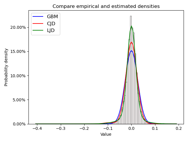
Blue is the geometric Brownian motion model (GBM), red is for the constant jump-diffusion model (CJD) and green is for the log-normal jump-diffusion model (LJD)
data/mle_params.csv
Following the fitting of theoretical models to empirical log-returns, the subsequent step involves calculating option prices. In the context of the constant jump diffusion model, equation (9) is utilized. It is important to note that this equation represents an infinite series, which poses numerical challenges for evaluation. Consequently, a finite series approximation is employed for practical purposes. An additional reason for considering a finite series is illustrated in the subsequent calculation. Let , where is defined in (13), then we obtain because
As a result of these calculations, we will fix the number of terms and truncate the remaining term when varying the second-order Esscher parameter .
As an example, we consider the parameters given in Table 2 where some of the values were taken from Table 1 above.
data/Esscher_pricing_interval_params.csv
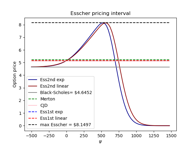
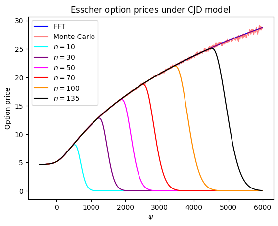
To determine an Essher pricing interval we calculate the Esscher prices for different values of using equation (9). We first consider the number of jumps to be . This number is motivated by Kou (2002) where the author calculates the price of an option with time to expiry of six months and suggests that numerically only the first 10 to 15 terms in the series are needed for most applications. While this is true for models such as Kou’s model and Merton’s model, it doesn’t hold true for our case with a free parameter where large values of yield inaccurate prices contradicting some of the theoretical results given in Proposition 2.5, see Figure 2 for example, where we observe first an increase of the option price with increasing parameter followed by a decrease to the value zero.
The behavior of the option price for this fixed number when and hence tends to infinity can be explained as follows. We use the terminology and notations from Proposition 2.5. Since the series is finite, the interchange between the sum and the limit is permissible in the sum , (13). For any , we find
with
hence and .
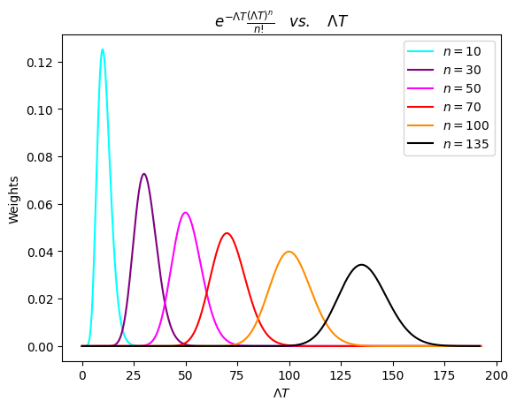
Thus, the remaining question is, how many terms to consider while increasing or equivalently and related to it how large is the Esscher pricing interval for a range of ? The option price can be seen as an infinite weighted average of Black-Scholes prices with weights for depending on and hence on . We analyse these weights as functions of . To simplify the notations we denote and consider , then it easily follows that
Thus, is a concave function of which reaches its maximum at and which tends to zero for tending to zero respectively to . This implies that we should choose in relation to the value of such that the terms with the highest weights are included. This implies that when increasing , and hence , more terms in the expansion should be used. This can also be financially motivated as is related to measuring the jump risk. Illustration of the behavior of the weights is given in Figure 3.
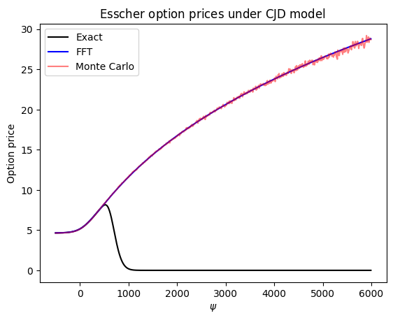
For extra validity of the Esscher pricing interval, we compare the pricing interval obtained by equation (9) with prices obtained by alternative methods such as Fast Fourier transform and Monte Carlo. The result of this comparison is illustrated in Figure 4 when we fix to and in Figure 5 when we add extra terms to the series in accordance to the previous argument.
2.3 A risk management application and comparison with other models
Using the MLE estimated parameters given in Table 1, we follow a similar idea to that in Kuen Siu et al. (2014), where we simulate P&L of a delta-hedging strategy under each different model and compare the 5% value-at-risk-metric (VaR) and expected shortfall (ES or conditional VaR). However, here, we also compare VaR and ES values for different choices of . VaR is a statistical measure widely used in financial risk management to assess the potential loss on a portfolio of financial assets over a specific time horizon, with a certain level of confidence. The calculation of VaR involves several key components such as the time horizon and the confidence level, whereas the ES is a risk measure that quantifies the expected loss of an investment portfolio in the worst-case scenario, given a certain level of confidence. The formula for calculating ES involves two components: the probability distribution and the threshold. For convenience, we illustrate the distributions of the hedging errors for the considered models in Figure 6.
data/Var_ES.csv
In Table 3, we list the VaR and ES of several models, namely, the geometric Brownian motion (GBM), the constant jump-diffusion (CJD) and the log-normal jump-diffusion (LJD). There are several cases under the CJD model all of which depend on how we choose the pricing measure. For example, the case of no jump risk means that the pricing measure for this case doesn’t consider jump risk (similar to Merton’s assumption) and the risk premium is the same as the Black-Scholes’ one, i.e., . Other cases of the CJD model are under the second-order Esscher measure except for the case when which retrieves the classical first-order Esscher. Note here that for calculating the options which produced the VaRs in Table 3 we fixed which is a valid choice according to the discussion in the previous subsection as the interval for is and doesn’t involve extreme values of .
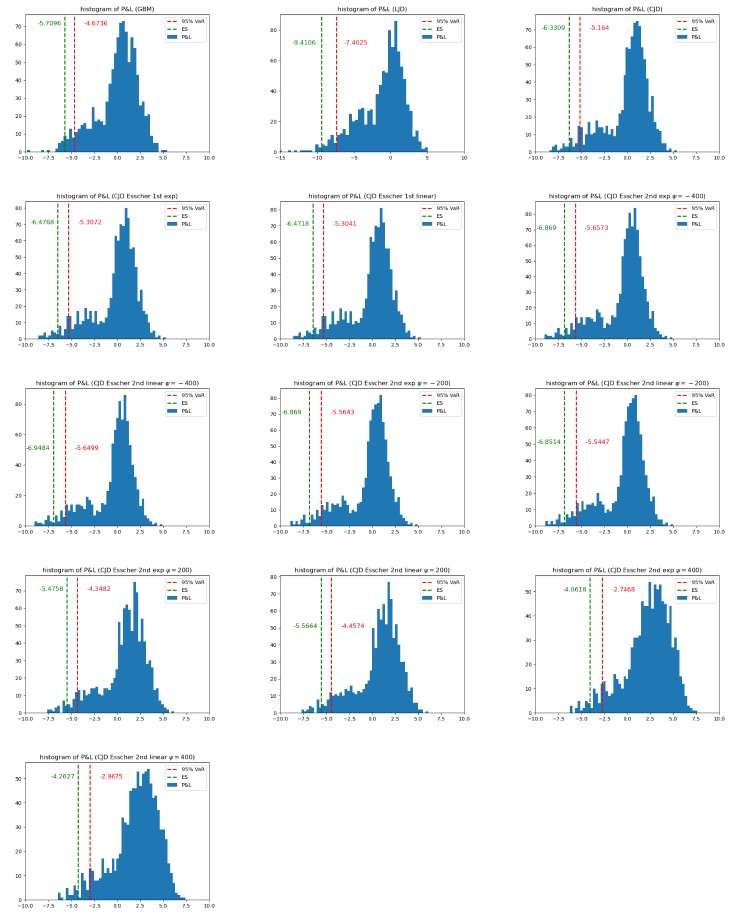
To interpret the values in Table 3, we take for example the case of the GBM. The VaR for the GBM model, means that there is a 5% probability that the portfolio will fall in value by more than $4.67 over the life of the option. The expected shortfall measures the average loss that exceeds the 5% VaR threshold. Thus, for the GBM case, it means that on average, losses exceeding the 5% VaR value is $5.71.
We can observe that for different (see Remark 2.3(1)), we can also obtain a range of VaRs and ESs for the same simple model. This flexibility allows risk managers to evaluate and manage risk exposure across various pricing scenarios of the option. Additionally, based on other internal risk considerations, such as liquidity constraints, operational risks, credit risk, etc., risk managers can select a that yields a risk measurement aligning with their risk appetite and these internal considerations. This approach enables a more tailored and comprehensive risk assessment strategy, beyond what is specified by the model dynamics alone.
We also notice that the VaR and ES of the LJD model are higher compared with the GBM and CJD models. This is due to the dynamics of the return process where the jumps are normally distributed with mean and variance . This allows the model to incorporate extreme values of the underlying due to jumps which are not captured by the constant jump in our constant jump diffusion model.
Next, we study how the Esscher pricing interval compares to other known models in the literature.
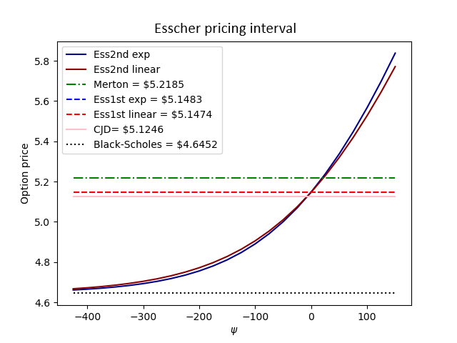
In Figure 7, we consider a pricing interval which corresponds to choosing . This interval seems enough to consider as it includes prices of models we are interested in comparing with the second-order Esscher price. We find that as becomes smaller, the option price approximates the Black-Scholes price, see Corollary 2.6. The model named CJD in Figure 7, is a jump-diffusion model with constant jump and where the jump risk is not priced (has the same risk premium as Black-Scholes’). Thus, due to the presence of jumps (adds more uncertainty to the model), it has a higher price compared to the Black-Scholes price. However, it has a lower value compared to a jump-diffusion model with constant jump and where the jump risk is priced using the classical first-order Esscher. Finally, we can see that even though the Merton’s jump-diffusion model does not price the jump risk, it has a higher price compared to the constant jump-diffusion model when the model prices the jump risk using the classical Esscher. This is due to the extra uncertainty which comes from the random jump sizes.
3 Second-order Esscher for other models
We start this section with a motivation for considering the second-order Esscher price under more complex models.
3.1 Motivation
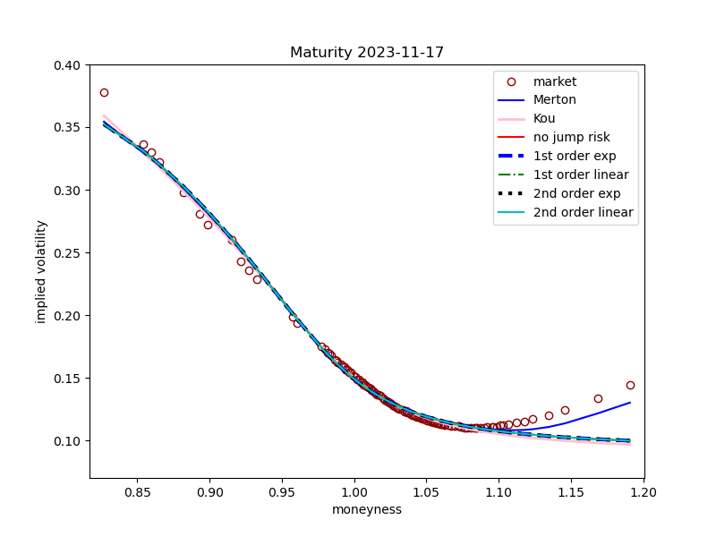
In this subsection, we assume that option market prices are available and we wish to calculate the implied volatilities using calibration. We consider the S&P 500 index from 2003-09-15 to 2023-09-16. We assume the trade date is 2023-09-15 with spot price $4,450.32. For the purpose of this paper, we consider only one maturity date which is 2023-11-17 to assess our model. We choose options with open interest higher than 100 and strike prices between $3,680 and $5,300. The calibration results are given in Table 4 below.
data/IV_params.csv
As we can see in Figure 8, the first-order and second-order Esscher do not have any advantage when calibrating and Merton’s model is better in capturing the volatility smile. This is due to the fact that jump-sizes in Merton’s model are random variables that are normally distributed. Hence, this allows for having extreme values for out-of-the-money options. The constant jump-diffusion model doesn’t have such flexibility and this limitation cannot be overcome by introducing the extra parameters from the first-order Esscher and and in the second-order Esscher pricing.
Due to this limitation we calculate option European options prices under more advanced models and we give the result in the next subsections.
Remark 3.1.
In the next subsections, we show the option prices of different models using their characteristic function under the second-order Esscher. Since it is not always possible to obtain an explicit formula for the option price, the use of the Fast Fourier transform algorithm (see Carr & Madan (1999)) is a convenient way to calculate the price. For a brief review of the Fourier transform method see Schmelzle (2010).
By the previous remark, we state the following
-
1.
The European call option price at time with ( is the strike price) and expiry time is under the second-order Esscher measure given by
where is a damping factor.
-
2.
The European put option price at time with ( is the strike price) and expiry time is under the second-order Esscher measure given by
where is a damping factor.
For each model, the only part that differs in calculating the call and put is the value of . This will be the focus of the following subsections.
3.2 Jump-diffusion models
We begin this subsection with the following assumption.
Assumptions 3.2.
Let be a Lévy process and be the Lévy measure of . Then, we assume that the following integrability condition holds,
For example, processes that satisfy this condition are the compound Poisson process and Variance Gamma process.
Throughout this subsection we consider the following model with constant parameters , and ,
| (14) |
with
and where the last term is a compound Poisson process in integral form (see (Jeanblanc et al., 2009, Chapter 8)), is the compensator of the Poisson process and with being the probability density function of the jump sizes.
We impose the following assumptions
Assumptions 3.3.
The Lévy measure satisfies Assumptions 3.2. Furthermore, the compensator of the process
exists, such that
is a local martingale, where is the compensated compound Poisson process and the deterministic function (depending on ) will be specified later.
Under this model, we have the following lemma.
Lemma 3.4.
Now, as a result of the latter lemma, the characteristic function under the second-order Esscher is determined in the following lemma.
Lemma 3.5.
In the next two subsections, we consider two well-known models which are special cases of the jump-diffusion in (14).
3.2.1 Log-normal jump-diffusion model
In this subsection we recall the log-normal model from Section 2. This model has the same form as (14), but with jump sizes that follow a normal distribution with mean and standard deviation , i.e,
| (16) |
where
By plugging the latter into (15), we can easily obtain the characteristic function, , under this model. Hence we have the following results.
Corollary 3.6.
For the model given in (16) the following assertions hold.
-
1.
is the Esscher density of order two for if and only if
and
-
2.
The characteristic function (15) of the exponential-Esscher can be calculated explicitly as
where
Furthermore, the case of the classical first-order Esscher can be retrieved by putting , i.e.,
(17)
Remark 3.7.
By the previous corollary, we have the following remarks.
- 1.
-
2.
In the case of Merton’s model, jump risk is not priced and the risk-neutral density is the same as for the Black-Scholes model with . Hence, the characteristic function of the Merton model is
-
3.
By the latter corollary, we observe that in the case of exponential-Esscher only one integral need to be numerically calculated. As for the case of linear-Esscher, we need to numerically calculate a double integral, as the integral in equation (15) is difficult to simplify for the exponential-Esscher counterpart. Thus, the linear-Esscher is expected to have less accuracy.
Explicit formula for the European option price
For the exponential-Esscher case we can calculate the explicit formula of the option price for the log-normal jump-diffusion model. To differentiate the exponential case, we put instead and use for . We begin with the following well-known result from the literature.
Lemma 3.8.
The compensator of the compound Poisson process is where .
Lemma 3.9.
The compensator of the compound Poisson process is where
with
and .
Proof.
Follows similarly to Lemma 3.8. ∎
We have the following corollary.
Corollary 3.10.
Consider the model given in (16). Then is an exponential-Esscher density of order two for if and only if
| (18) |
and
where the cumulant function is
Proof.
Follows similar to the general semimartingale case given in Choulli et al. (2024). ∎
Theorem 3.11.
For the model given in (16) the following assertions hold.
-
(a)
The explicit price of a European call option under the second-order Esscher measure when the jump size is normally distributed is calculated as follows.
where
and
-
(b)
In particular, when we obtain the explicit solution of the price equation under the classical Esscher where , and .
Proof.
See Appendix A.1. ∎
Corollary 3.12.
For the model given in (16) the following assertions hold.
-
(a)
The explicit price of a European call option under the first-order Esscher (i.e., ) measure when the jump size is normally distributed is calculated as follows.
where
-
(b)
In particular, when and , we retrieve the case of constant jumps discussed in Section 2 of this paper.
Remark 3.13.
Finding an explicit solution for the European option price under the linear-Esscher measure is not an easy task. The reason for this is that the probability density function is difficult to obtain. Therefore the Fourier transform discussed earlier in this subsection is an alternative method to obtain an equation in a closed form for the option price.
3.2.2 Double-exponential jump-diffusion model
Similar to the previous subsection, the double-exponential jump-diffusion model shares the same form of the log-return process with the only difference that the jumps sizes have a Double Exponential distribution with parameters , , and , i.e,
| (19) |
where
Corollary 3.14.
Consider the model given in (19). Then, the following assertions hold.
-
1.
is the Esscher density of order two for if and only if
(20) and
-
2.
The characteristics function of the Exponential Esscher can be calculated explicitly as
where and
Furthermore, the case of classical Esscher can be retrieved by putting , i.e.,
(21) where is the unique solution of the martingale equation (20) when and satisfies .
Proof.
In order to prove Assertion 2 of the corollary, we only need to focus on the integral which is equal to
where
For the improper integrals to be well defined the parameter should be negative. By completing the square and introducing and with , we get
By similar steps putting we find for ,
For the case when , it is easy to check that
This integral exists only when and for and . Thus, equivalently, this integral exists when as . ∎
Remark 3.15.
A few remarks regarding the latter corollary.
- 1.
-
2.
Unlike the case with log-normal jumps, we cannot retrieve the classical first-order Esscher by substituting in .
-
3.
Under the same risk-neutral measure as for the Black-Scholes model we get the following characteristic function for Kou’s double exponential jump-diffusion model:
see for example Håkansson (2015).
3.3 Variance Gamma model
A Variance Gamma process is obtained by evaluating a Brownian motion with a drift at a random time given by a gamma process, see Madan et al. (1998).
Definition 3.16.
The Variance Gamma process with parameters is defined as
where is a standard Brownian motion and is a gamma process with unit mean rate and variance rate .
Under this subsection, we consider the asymmetric Variance Gamma model with drift as in Madan et al. (1998) to describe the Lévy process ,
| (22) |
where
The case when is called the symmetric Variance Gamma process Madan & Milne (1991). By the Lévy-Itô decomposition and Assumption 3.2, we can write (22) as
| (23) |
Before stating our next corollary, we state the following assumption and recall Proposition 11.2.2.5 from Jeanblanc et al. (2009).
Assumptions 3.17.
The Lévy measure satisfies Assumptions 3.2. Furthermore, the compensator of the process
exists, such that
is a local martingale.
Notice that the process
is a martingale, i.e., is the compensator of the process .
Proposition 3.18.
Let be a Lévy process and its Lévy measure. For every and every Borel function defined on such that , one has
Corollary 3.19.
Proof.
Assertion 1 follows by noticing that the Lévy process given in (23) is a special case of the semimartingale case discussed in Choulli et al. (2024).
To prove Assertion 2, we focus on the exponential Esscher i.e., and . By the Doléans-Dade exponential and (22), the exponential-Esscher martingale can be written as
Equivalently, by using (23), we have
Hence,
By applying the result in Proposition 3.18 to given in (23) yields,
For the classical Esscher where we get the same result as in Salhi (2017) by noticing that
where . This ends the proof. ∎
4 Conclusion
From the analysis presented in Section 2, it becomes clear that the introduction of an additional free parameter provides a valuable mechanism for incorporating a broader spectrum of financial information into the model. This parameter allows us to embed crucial data related to various types of risks, without necessitating the adoption of more complex dynamics. By leveraging this additional parameter, we can seamlessly integrate considerations such as liquidity risk, credit risk, extra sources of uncertainty, etc., into the model. This approach not only enhances the model’s flexibility and robustness but also enables a more nuanced and comprehensive risk assessment, addressing factors that may not be explicitly captured by the primary model dynamics. This integration of extra financial information ultimately leads to a more strategic decision-making process in risk management and OTC option pricing. In Section 3, we have presented formulas for calculating option prices under different models using the Fourier transform method. The examples presented here, extend the characteristic function under the classical Esscher, which is well-studied in the literature, to the characteristic function under the second-order Esscher. Further models such as the normal inverse Gaussian, stochastic variance and regime switching are studied under the second-order Esscher in Elazkany (2025).
Appendix A Proofs
A.1 Proof of Theorem 3.11
By Corollary 3.10 and the definition of the Doléans-Dade exponential we have the following
| (24) |
Hence, given the model (16), we have
By the martingale condition (18), we have
Therefore,
Next and throughout the proof we will apply the same technique used by Merton (1976), that is, having where is a standard normal random variable, and conditioning on the number of jumps we have . Hence,
Therefore, by putting , we have in distributional sense
| (25) |
Using the above, the martingale condition (18) becomes
| (26) |
Now, we calculate the European call option price under the second-order Esscher martingale measure.
| (27) |
Before proceeding with calculating the conditional expectations in the above, let’s simplify the set when conditioned by the number of jumps. We find
By (25), we have
where
and by adding and subtracting , we get
Now, let’s calculate the following expectation
By (24), we get
and by (25)
Since is standard normally distributed, then
Let
then
By changing the variable, we find for ,
and
By the martingale condition (26), we obtain
where
Hence,
| (28) |
In a similar fashion, we calculate for ,
| (29) | ||||
where
and
Substituting (A.1) and (A.1) in (A.1) leads to the stated result. ∎
References
- (1)
- Benth et al. (2008) Benth, F. E., Benth, J. S. & Koekebakker, S. (2008), Stochastic modelling of electricity and related markets, Vol. 11, World Scientific.
- Benth & Sgarra (2012) Benth, F. E. & Sgarra, C. (2012), ‘The risk premium and the esscher transform in power markets’, Stochastic Analysis and Applications 30(1), 20–43.
- Bondi et al. (2020) Bondi, A., Radojičić, D. & Rheinländer, T. (2020), ‘Comparing two different option pricing methods’, Risks 8(4), 108.
- Boughamoura & Trabelsi (2014) Boughamoura, W. & Trabelsi, F. (2014), ‘On two-parametric Esscher transform for geometric CGMY Lévy processes’, International Journal of Operational Research 19(3), 280–301.
- Carr & Madan (1999) Carr, P. & Madan, D. (1999), ‘Option valuation using the fast Fourier transform’, Journal of Computational Finance 2(4), 61–73.
- Choulli et al. (2024) Choulli, T., Elazkany, E. & Vanmaele, M. (2024), ‘The second-order Esscher martingale densities for continuous-time market models’, arXiv preprint arXiv:2407.03960 .
- Eberlein & Jacod (1997) Eberlein, E. & Jacod, J. (1997), ‘On the range of options prices’, Finance and Stochastics 1(2), 131–140.
- Elazkany (2025) Elazkany, E. (2025), Esscher pricing methods for models under random horizon: Theory and Computational Methods, Thesis in progress, University of Alberta.
- Feng & Linetsky (2008) Feng, L. & Linetsky, V. (2008), ‘Pricing options in jump-diffusion models: An extrapolation approach’, Operations Research 56(2), 304–325.
- Håkansson (2015) Håkansson, J. (2015), Option pricing and exponential Lévy models, Master’s thesis, adv. P. Albin, Chalmers University of Technology.
- Hilliard & Reis (1998) Hilliard, J. E. & Reis, J. (1998), ‘Valuation of commodity futures and options under stochastic convenience yields, interest rates, and jump diffusions in the spot’, Journal of Financial and Quantitative Analysis 33(1), 61–86.
- Jeanblanc et al. (2009) Jeanblanc, M., Yor, M. & Chesney, M. (2009), Mathematical Methods for Financial Markets, Springer Science & Business Media.
- Kou (2002) Kou, S. G. (2002), ‘A jump-diffusion model for option pricing’, Management science 48(8), 1086–1101.
- Kuen Siu et al. (2014) Kuen Siu, T., Nawar, R. & Ewald, C. O. (2014), ‘Hedging crude oil derivatives in GARCH-type models’, Journal of Energy Markets 7(1).
- Madan et al. (1998) Madan, D. B., Carr, P. P. & Chang, E. C. (1998), ‘The Variance Gamma process and option pricing’, Review of Finance 2(1), 79–105.
- Madan & Milne (1991) Madan, D. B. & Milne, F. (1991), ‘Option pricing with VG martingale components’, Mathematical Finance 1(4), 39–55.
- Matsuda (2004) Matsuda, K. (2004), ‘Introduction to Merton jump diffusion model’, Department of Economics, The Graduate Center, The City University of New York, New York .
- Méndez Lara (2017) Méndez Lara, Ó. A. (2017), Application of the perturbation method to valuation problems of European options, Master’s thesis, Centro de Investigación y de Estudios Avanzados del IPN.
- Merton (1976) Merton, R. C. (1976), ‘Option pricing when underlying stock returns are discontinuous’, Journal of Financial Economics 3(1-2), 125–144.
- Monfort & Pegoraro (2012) Monfort, A. & Pegoraro, F. (2012), ‘Asset pricing with second-order Esscher transforms’, Journal of Banking & Finance 36(6), 1678–1687.
- Salhi (2017) Salhi, K. (2017), ‘Pricing European options and risk measurement under exponential Lévy models: A practical guide’, International Journal of Financial Engineering 4(02n03), 1750016.
- Schmelzle (2010) Schmelzle, M. (2010), ‘Option pricing formulae using Fourier transform: Theory and application’, Preprint, http://pfadintegral. com .