Faster Local Solvers for Graph Diffusion Equations
Abstract
Efficient computation of graph diffusion equations (GDEs), such as Personalized PageRank, Katz centrality, and the Heat kernel, is crucial for clustering, training neural networks, and many other graph-related problems. Standard iterative methods require accessing the whole graph per iteration, making them time-consuming for large-scale graphs. While existing local solvers approximate diffusion vectors through heuristic local updates, they often operate sequentially and are typically designed for specific diffusion types, limiting their applicability. Given that diffusion vectors are highly localizable, as measured by the participation ratio, this paper introduces a novel framework for approximately solving GDEs using a local diffusion process. This framework reveals the suboptimality of existing local solvers. Furthermore, our approach effectively localizes standard iterative solvers by designing simple and provably sublinear time algorithms. These new local solvers are highly parallelizable, making them well-suited for implementation on GPUs. We demonstrate the effectiveness of our framework in quickly obtaining approximate diffusion vectors, achieving up to a hundred-fold speed improvement, and its applicability to large-scale dynamic graphs. Our framework could also facilitate more efficient local message-passing mechanisms for GNNs.
1 Introduction
Graph diffusion equations (GDEs), such as Personalized PageRank (PPR) [41, 44, 62], Katz centrality (Katz) [46], Heat kernel (HK) [21], and Inverse PageRank (IPR) [51], are fundamental tools for modeling graph data. These score vectors for nodes in a graph capture various aspects of their importance or influence. They have been successfully applied to many graph learning tasks including local clustering [1, 81], detecting communities [49], semi-supervised learning [78, 80], node embeddings [63, 67], training graph neural networks (GNNs) [9, 16, 19, 31, 75], and many other applications [32]. Specifically, given a propagation matrix associated with an undirected graph , a general graph diffusion equation is defined as
| (1) |
where is the diffusion vector computed from a source vector , and the sequence of coefficients satisfies . Equation (1) represents a system of linear, constant-coefficient ordinary differential equation, , with an initial condition and . Standard solvers [34, 57] for computing require access to matrix-vector product operations , typically involving operations, where is the total number of edges in . This could be time-consuming when dealing with large-scale graphs [42].
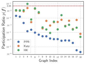
A key property of is the high localization of its entry magnitudes, which reside in a small portion of . Figure 1 demonstrates this localization property of on PPR, Katz, and HK. Leveraging this locality property allows for more efficient approximation using local iterative solvers, which heuristically
avoid operations. Local push-based methods [1, 7, 49] or their variants [3, 12] are known to be closely related to Gauss-Seidel [49, 18]. However, current local push-based methods are fundamentally sequential iterative solvers and focused on specific types such as PPR or HK. These disadvantages limit their applicability to modern GPU architectures and their generalizability.
By leveraging the locality of , we propose, for the first time, a general local iterative framework for solving GDEs using a local diffusion process. A novel component of our framework is to model local diffusion as a locally evolving set process inspired by its stochastic counterpart [58]. We use this framework to localize commonly used standard solvers, demonstrating faster local methods for approximating . For example, the local gradient descent is simple, provably sublinear, and highly parallelizable. It can be accelerated further by using local momentum. Our contributions are
-
–
By demonstrating that popular diffusion vectors, such as PPR, Katz, and HK, have strong localization properties using the participation ratio, we propose a novel graph diffusion framework via a local diffusion process for efficiently approximating GDEs. This framework effectively tracks most energy during diffusion while maintaining local computation.
-
–
To demonstrate the power of our proposed framework, we prove that APPR [1], a widely used local push-based algorithm, can be treated as a special case. We provide better diffusion-based bounds where is a lower bound of . This bound is effective for both PPR and Katz and is empirically smaller than , previously well-known for APPR.
-
–
We design simple and fast local methods based on standard gradient descent for APPR and Katz, which admit runtime bounds of for both cases. These methods are GPU-friendly, and we demonstrate that this iterative solution is significantly faster on GPU architecture compared to APPR. When the propagation matrix is symmetric, we show that this local method can be accelerated further using the local Chebyshev method for PPR and Katz.
-
–
Experimental results on GDE approximation of PPR, HK, and Katz demonstrate that these local solvers significantly accelerate their standard counterparts. We further show that they can be naturally adopted to approximate dynamic diffusion vectors. Our experiments indicate that these local methods for training are twice as fast as standard PPR-based GNNs. These results may suggest a novel local message-passing approach to train commonly used GNNs.
All proofs, detailed experimental settings, and related works are postponed to the appendix. Our code is publicly available at https://github.com/JiaheBai/Faster-Local-Solver-for-GDEs.
2 GDEs, Localization, and Existing Local Solvers
| Equ. | |||
|---|---|---|---|
| PPR [62] | |||
| Katz [46] | |||
| HK [21] | |||
| IPR [51] | |||
| APPNP [30] |
Notations. We consider an undirected graph where is the set of nodes, and is the edge set with . The degree matrix is , and is the adjacency matrix of . The volume of subset nodes is . The set of neighbors of node is denoted by . The standard basis for node is . The support of is defined as .
Many graph learning tools can be represented as diffusion vectors. Table 1 presents examples widely used as graph learning tools. The coefficient usually exhibits exponential decay, so most of the energy of is related to only the first few . We revisit these GDEs and existing local solvers.
Personalized PageRank. Given the weight decaying strategy and a predefined damping factor with , the analytic solution for PPR is
| (2) |
These vectors can be used to find a local graph cut or train GNNs [10, 9, 25, 79]. The well-known approximate PPR (APPR) method [1] locally updates the estimate-residual pair as follows
Here, each active node has a large residual with initial values and . The runtime bound for reaching for all nodes is graph-independent and is , leveraging the monotonicity property. Previous analyses [49, 18] suggest that APPR is a localized version of the Gauss-Seidel (GS) iteration and thus has fundamental sequential limitations.
Katz centrality. Given the weight with and a different propagation matrix . The solution for Katz centrality can then be rewritten as:
| (3) |
The goal is to approximate the Katz centrality . Similar to APPR, a local solver [11] for Katz centrality, denoted as AKatz, can be designed as follows
AKatz is a coordinate descent method [11]. Under the nonnegativity assumption of (i.e., ), a convergence bound for the residual is provided.
Heat Kernel. The heat kernel (HK) [21] is useful for finding smaller but more precise local graph cuts. It uses a different weight decaying and the vector is then defined as
where is the temperature parameter of the HK equation and . Unlike the previous two, this equation does not admit an analytic solution. Following the technique developed in [48, 49], given an initial vector and temperature , the HK vector can be approximated using the first terms of the Taylor polynomial approximation: define with and for . It is known that . This is equivalent to solving the linear system , where denotes the Kronecker product. Then, the push-based method, namely AHK, has the following updates
There are many other types of GDEs, such as Inverse PageRank [51], which generalize PPR. Many GNN propagation layers, such as SGC [69] and APPNP [30], can be formulated as GDEs. For all these , we use the participation ratio [54] to measure its localization ability, defined as
When the entries in are uniformly distributed, such that , then . However, in the extremely sparse case where is a standard basis vector, indicates the sparsity effect. Figure 1 illustrates the participation ratios, showing that almost all vectors have ratios below 0.01. Additionally, larger graphs tend to have smaller participation ratios.
APPR, AKatz, and AHK all have fundamental limitations due to their reliance on sequential Gauss-Seidel-style updates, which limit their parallelization ability. In the following sections, we will develop faster local methods using the local diffusion framework for solving PPR and Katz.
3 Faster Solvers via Local Diffusion Process
We introduce a local diffusion process framework, which allows standard iterative solvers to be effectively localized. By incorporating this framework, we show that the computation of PPR and Katz defined in (2) and (3) can be locally approximated sequentially or in parallel on GPUs.
3.1 Local diffusion process
To compute and , it is equivalent to solving the linear systems, which can be written as
| (4) |
where is a (symmetric) positive definite matrix with eigenvalues bounded by and , i.e., . For PPR, we solve , which is equivalent to solving . For Katz, we compute . The vector is sparse, with . We define local diffusion process, a locally evolving set procedure inspired by its stochastic counterpart [58] as follows
Definition 3.1 (Local diffusion process).
Given an input graph , a source distribution , precision tolerance , and a local iterative method with parameter for solving (4), the local diffusion process is defined as a process of updates . Specifically, it follows the dynamic system
| (5) |
where is a mapping via some iterative solver . For all three diffusion processes (PPR, Katz, and HK), we set . We say this process converges when if there exists such ; the generated sequence of active nodes are . The total number of operations of the local solver is
where we denote the average of active volume as .
Intuitively, we can treat this local diffusion process as a random walk on a Markov Chain defined on the space of all subsets of , where the transition probability represents the operation cost. More efficient local solvers try to find a shorter random walk from to . The following two subsections demonstrate the power of this process in designing local methods for PPR and Katz.
3.2 Sequential local updates via Successive Overrelaxation (SOR)
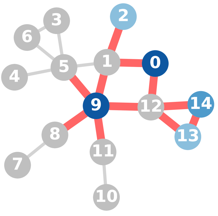
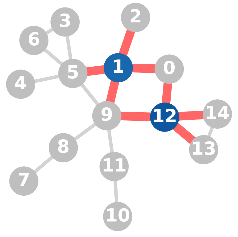
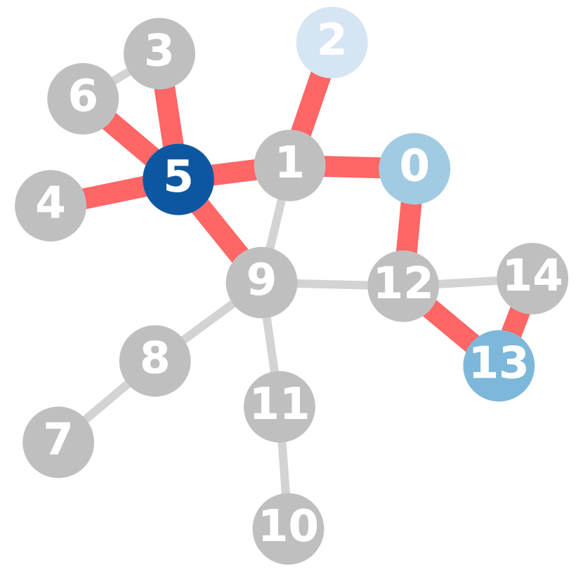
Given the estimate at -th iteration, we define residual and be the matrix induced by and . The typical local Gauss-Seidel with Successive Overrelaxation has the following online estimate-residual updates (See Section 11.2 of [34]): at each time , for each active node with , we update each -th entry of and corresponding residual as the following
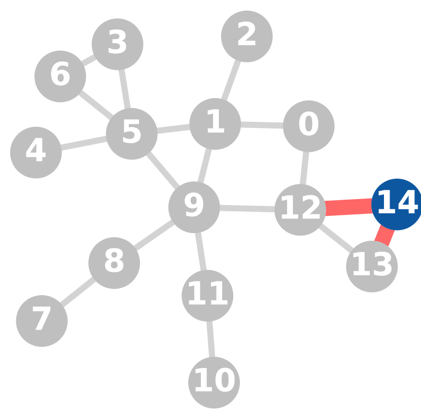
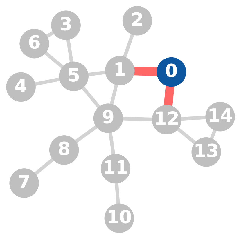
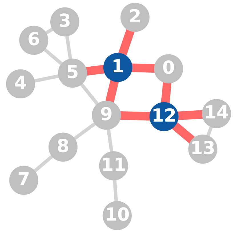
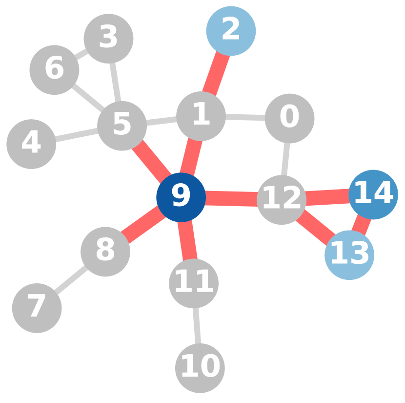
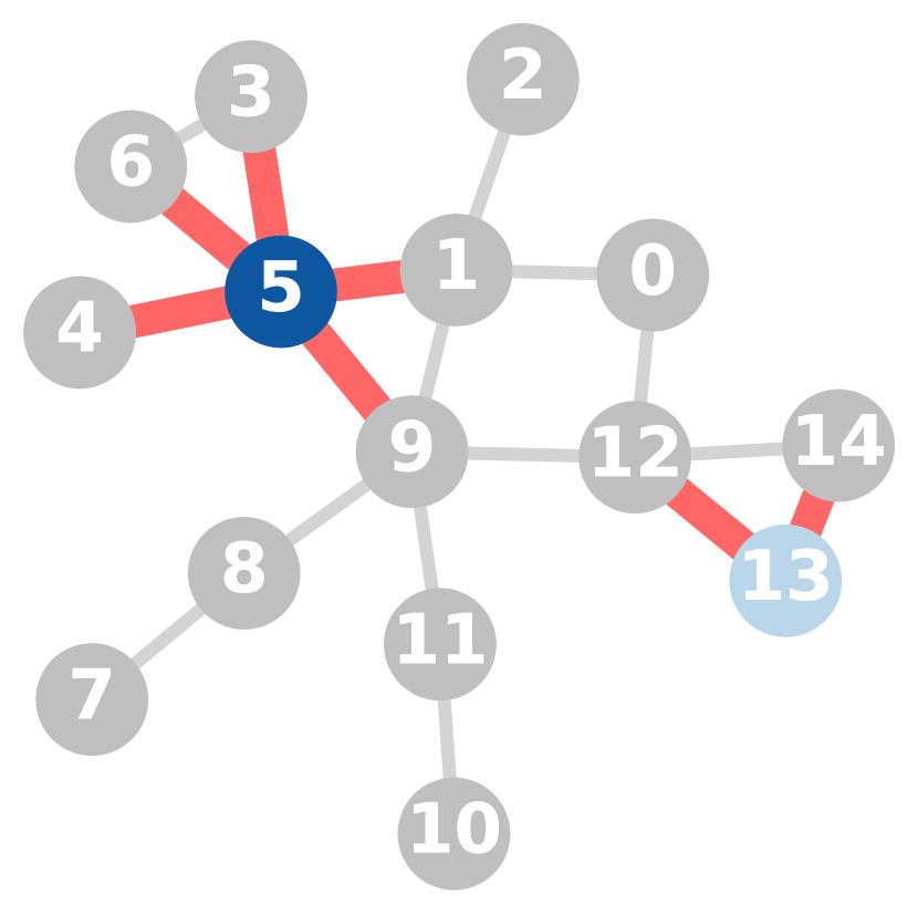
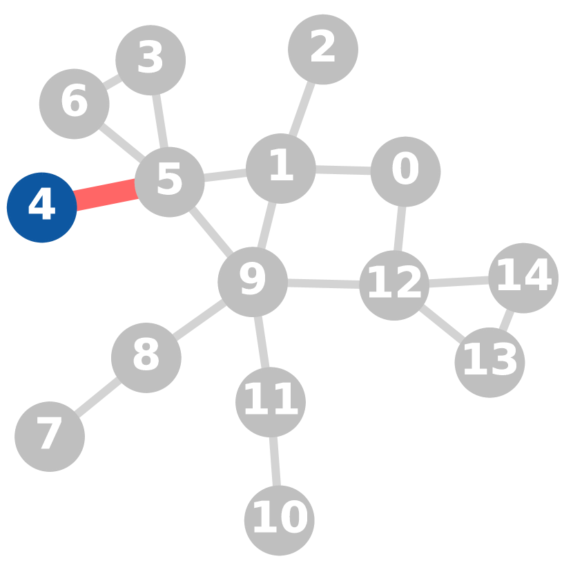
(6) where is the current time, and update unit vector is . Note that each update of (6) is . If , it reduces to the standard GS-SOR [34]. Therefore, APPR is a special case of (6), a local variant of GS-SOR with . Figure 2 illustrates this procedure. APPR updates at some entries and keeps track of large magnitudes of per iteration, while LocalSOR allows for a better choice of ; hence, the total number of operations is reduced. We establish the following fundamental property of LocalSOR.


Theorem 3.2 (Properties of local diffusion process via LocalSOR).
Let where and if ; 0 otherwise. Define maximal value . Assume that is nonnegative and , are such that , given the updates of (6), then the local diffusion process of with has the following properties
-
1.
Nonnegativity. for all and with .
-
2.
Monotonicity property. .
If the local diffusion process converges (i.e., ), then is bounded by
Based on Theorem 3.2, we establish the following sublinear time bounds of LocalSOR for PPR.
Theorem 3.3 (Sublinear runtime bound of LocalSOR for PPR).
Let . Given an undirected graph and a target source node with , and provided , the run time of LocalSOR in Equ. (6) for solving with the stop condition and initials and is bounded as the following
| (7) |
where . The estimate satisfies .
The above theorem demonstrates the usefulness of our framework. It shows a new evolving bound where as long as satisfying certain assumption (It is true for PPR and Katz). Similarly, applying Theorem 3.2, we have the following result for approximating .
Corollary 3.4 (Runtime bound of LocalSOR for Katz).
Let and . Given an undirected graph and a target source node with , and provided , the run time of LocalSOR in Equ. (6) for solving with the stop condition and initials and is bounded as the following
| (8) |
The estimate satisfies .
Accerlation when is Stieltjes matrix (). It is well-known that when , GS-SOR has acceleration ability when is Stieltjes. However, it is fundamentally difficult to prove the runtime bound as the monotonicity property no longer holds. It has been conjectured that a runtime of can be achieved [27]. Incorporating our bound, a new conjecture could be : If is Stieltjes, then with the proper choice of , one can achieve speedup convergence to ? We leave it as an open problem.
3.3 Parallelizable local updates via GD and Chebyshev
The fundamental limitation of LocalSOR is its reliance on essentially sequential online updates, which may be challenging to utilize with GPU-type computing resources. Interestingly, we developed a local iterative method that is embarrassingly simpler, highly parallelizable, and provably sublinear for approximating PPR and Katz. First, one can reformulate the equation of PPR and Katz as 111For the PPR equation, , we can symmetrize this linear system by rewriting it as . The solution is then recovered by .
| (9) |
A natural idea for solving the above is to use standard GD. Hence, following a similar idea of local updates, we simultaneously update solutions for . We propose the following local GD.
(10)
Theorem 3.5 (Properties of local diffusion process via LocalGD).
Let where and if ; 0 otherwise. Define maximal value . Assume that and , are such that , given the updates of (10), then the local diffusion process of has the following properties
-
1.
Nonnegativity. for all .
-
2.
Monotonicity property.
If the local diffusion process converges (i.e., ), then is bounded by
Indeed, the above local updates have properties that are quite similar to those of SOR. Based on Theorem 3.5, we establish the sublinear runtime bounds of LocalGD for solving PPR and Katz.
Corollary 3.6 (Convergence of LocalGD for PPR and Katz).
Let and . Use LocalGD to approximate PPR or Katz by using iterative procedure (10). Denote and as the total number of operations needed by using LocalGD, they can then be bounded by
| (11) |
for a stop condition . For solving Katz, then the toal runtime is bounded by
| (12) |
for a stop condition . The estimate of equality is the same as that of LocalSOR.
Remark 3.7.
Note that LocalGD is quite different from iterative hard-thresholding methods [43] where the time complexity of the thresholding operator is at best, hence not a sublinear algorithm.
Accerlerated local Chevbyshev. One can extend the Chebyshev method [39], an optimal iterative solver for (9). Following [24], Chebyshev polynomials are defined via following recursions
| (13) |
Given , the standard Chevyshev method is defined as
where . For example, for approximating PPR, we propose the following local updates
The sublinear runtime analysis for LocalCH is complicated since it does not follow the monotonicity property during the updates. Whether it admits, an accelerated rate remains an open problem.
4 Applications to Dynamic GDEs and GNN Propagation
Our accelerated local solvers are ready for many applications. We demonstrate here that they can be incorporated to approximate dynamic GDEs and GNN propagation. We consider the discrete-time dynamic graph [47] which contains a sequence of snapshots of the underlying graphs, i.e., . The transition from to consists of a list of events involving edge deletions or insertions. The graph is then represented as: . The goal is to calculate an approximate for the PPR linear system at time . That is,
| (14) |
The key advantage of updating the above equation (presented in Algorithm 3) is that the APPR algorithm is used as a primary component for updating, making it much cheaper than computing from scratch. Consequently, we can apply our local solver LocalSOR to the above equation, and we found that it significantly sped up dynamic GDE calculations and dynamic PPR-based GNN training.
5 Experiments
Datasets. We conduct experiments on 18 graphs ranging from small-scale (cora) to large-scale (papers100M), mainly collected from Stanford SNAP [45] and OGB [42] (see details in Table 3). We focus on the following tasks: 1) approximating diffusion vectors with fixed stop conditions using both CPU and GPU implementations; 2) approximating dynamic PPR using local methods and training dynamic GNN models based on InstantGNN models [75]. 222More detailed experimental setups and additional results are in the appendix.
Baselines and Experimental Setups. We consider four methods with their localized counterparts: Gauss-Seidel (GS)/LocalGS, Successive Overrelaxation (SOR)/LocalSOR, Gradient Descent (GD)/LocalGD, and Chebyshev (CH)/LocalCH.333Note that the approximate local solvers of APPR, AHK, and AKatz will be referred to as GS. Specifically, we use the stop condition for PPR and for Katz, while we follow the parameter settings used in [49] for HK. For LocalSOR, we use the optimal parameter suggested in Section 3.2. We randomly sample 50 nodes uniformly from lower to higher-degree nodes for all experiments. All results are averaged over these 50 nodes. We conduct experiments using Python 3.10 with CuPy and Numba on a server with 80 cores, 256GB of memory, and two 28GB NVIDIA-4090 GPUs.
5.1 Results on efficiency of local GDE solvers
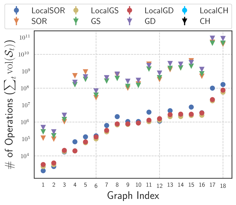
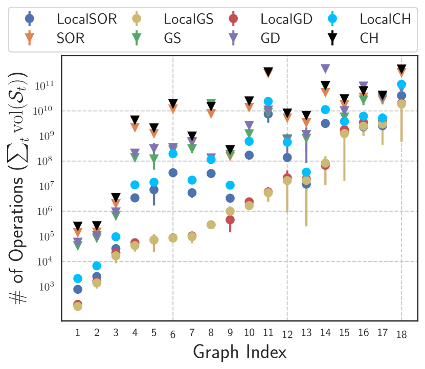
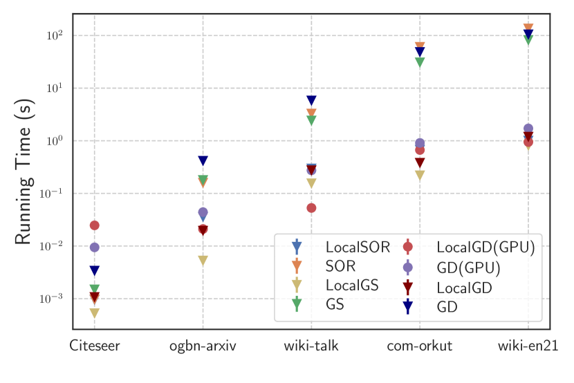
Local solvers are faster and use fewer operations. We first investigate the efficiency of the proposed local solvers for computing PPR and Katz centrality. We set for PPR and for Katz. We use a temperature of and for HK. All algorithms for HK estimate the number of iterations by considering the truncated error of Taylor approximation. Table 2 presents the speedup ratio of four local methods over their standard counterparts. For five graph datasets, the speedup is more than 100 times in terms of the number of operations in most cases. This strongly demonstrates the efficiency of these local solvers. Figure 4 presents all such results. Key observations are: 1) All local methods significantly speed up their global counterparts on all datasets. This strongly indicates that when is within a certain range, local solvers for GDEs are much cheaper than their global counterparts. 2) Among all local methods, LocalGS and LocalGD have the best overall performance. This may seem counterintuitive since LocalSOR and LocalCH are more efficient in convergence rate. However, the number of iterations needed for or is much smaller. Hence, their improvements are less significant.
| Graph | SOR/LocalSOR | GS/LocalGS | GD/LocalGD | CH/LocalCH |
| Citeseer | 86.21 | 114.89 | 157.41 | 5.86 |
| ogbn-arxiv | 183.43 | 392.26 | 528.03 | 101.88 |
| ogbn-products | 667.39 | 765.97 | 904.21 | 417.41 |
| wiki-talk | 169.67 | 172.95 | 336.53 | 30.45 |
| ogbn-papers100M | 243.68 | 809.47 | 1137.41 | 131.30 |
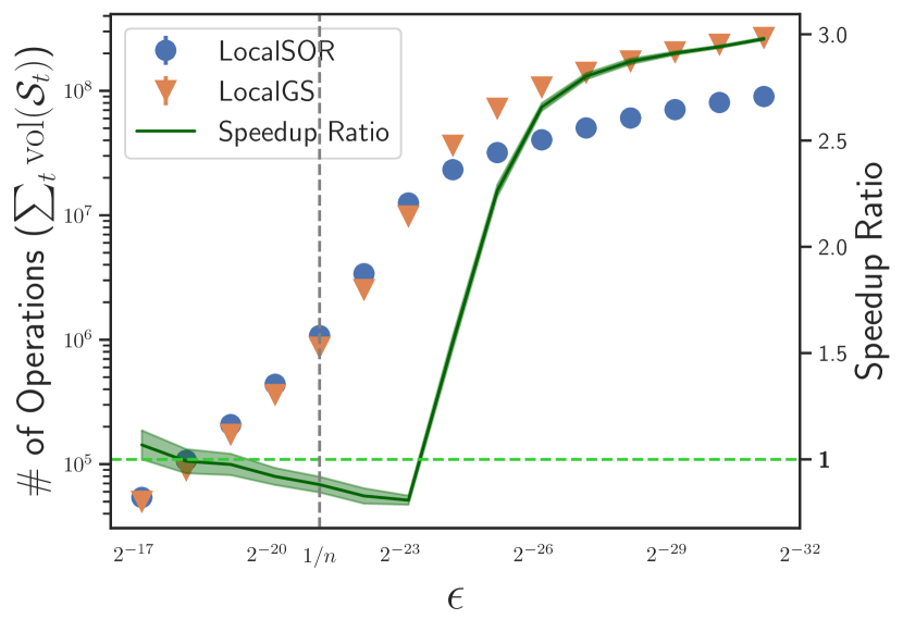
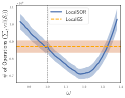
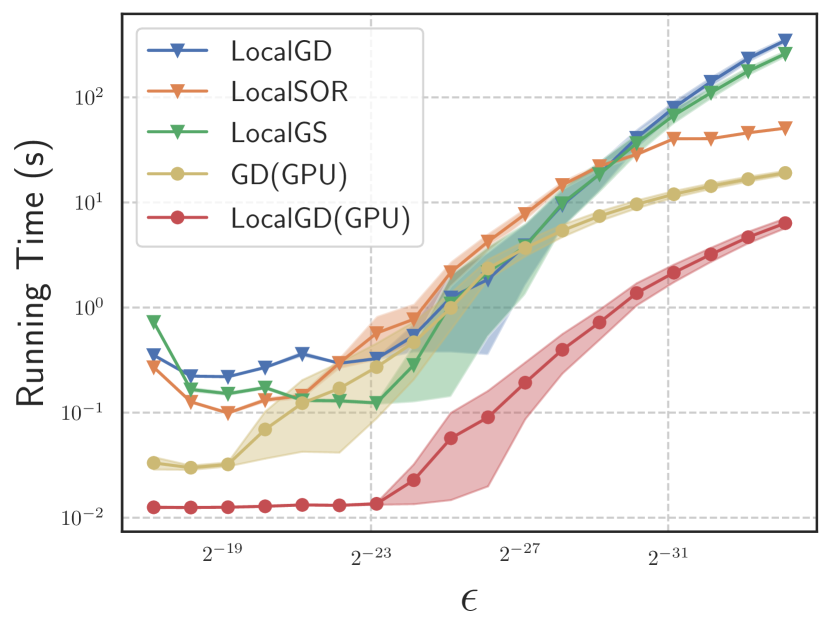
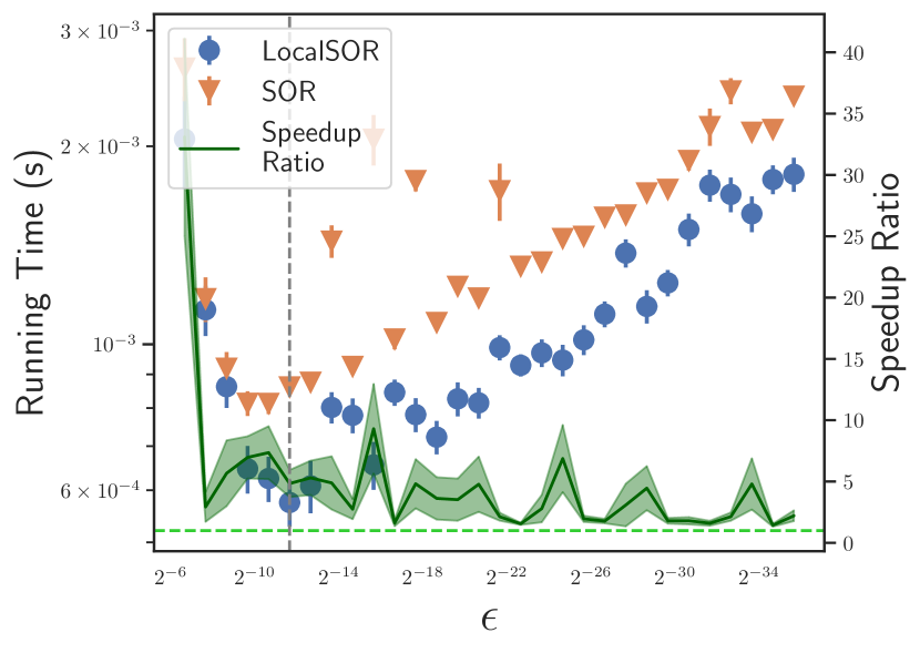
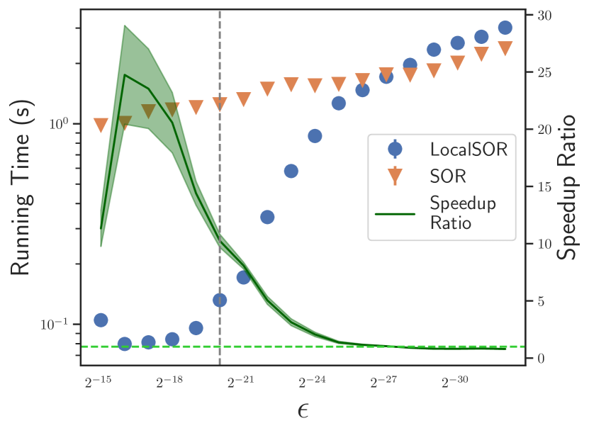
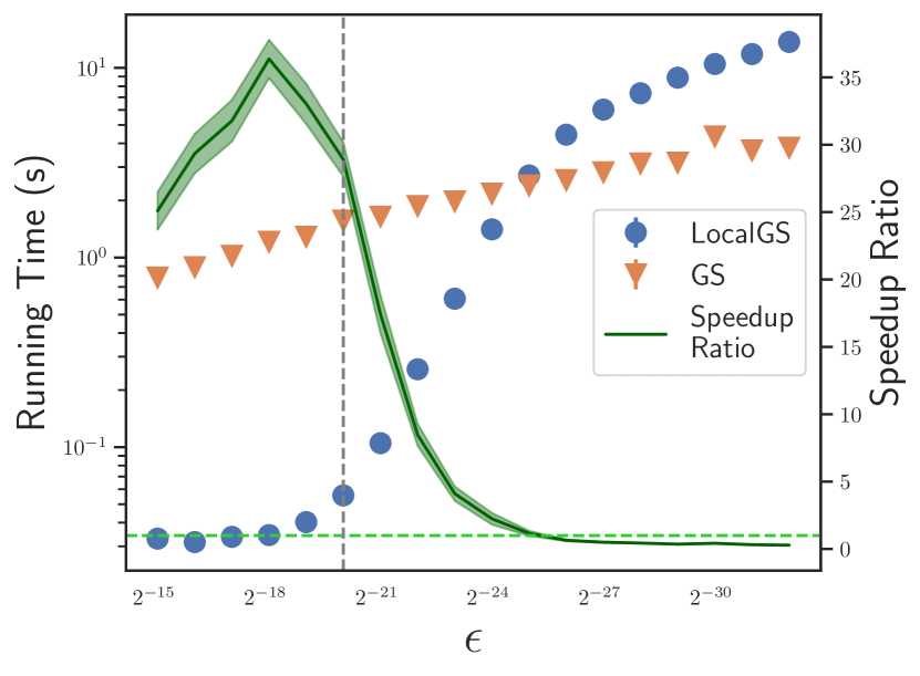
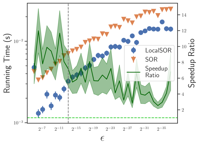
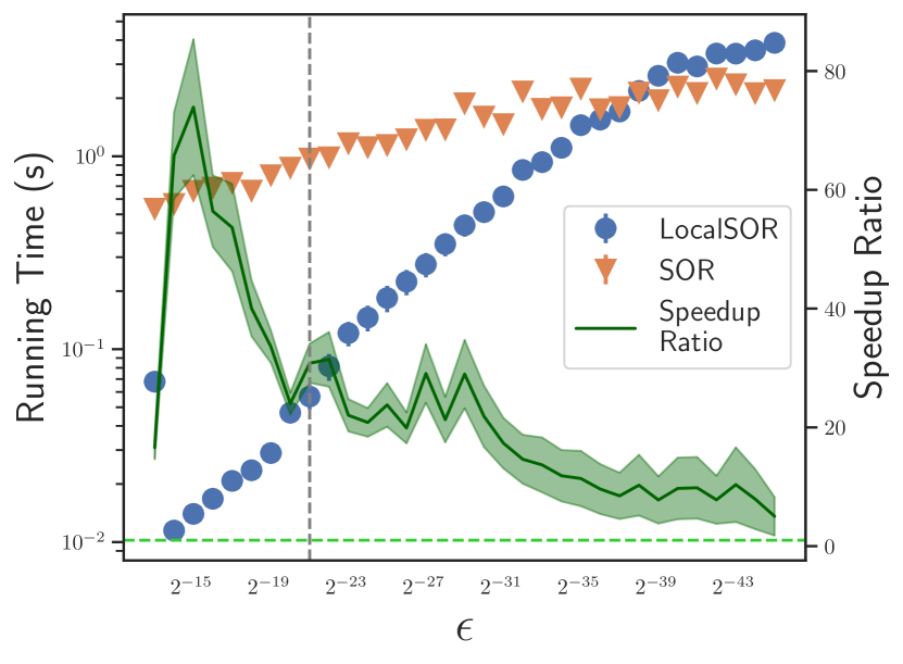
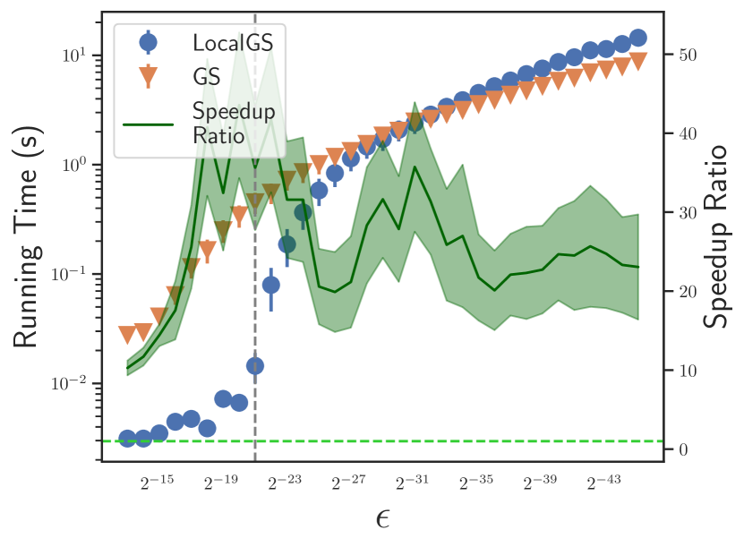
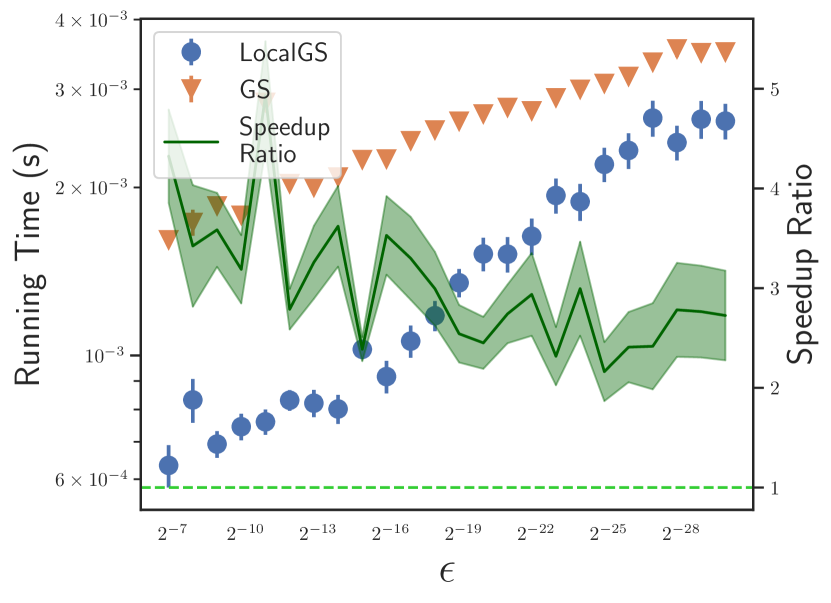
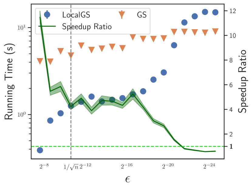
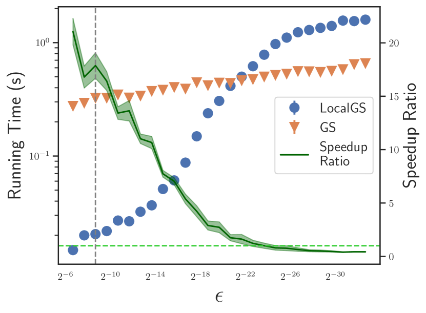
Which local GDE solvers are the best under what settings? In the lower precision setting, previous results suggest that LocalSOR and LocalGD perform best overall. To test the proposed LocalSOR efficiency, we use the ogbn-arxiv dataset to evaluate the local algorithm efficiency under a high precision setting. Figure 5 illustrates the performance of LocalSOR and LocalGS for PPR and Katz. As becomes smaller, the speedup of LocalSOR over LocalGS becomes more significant.
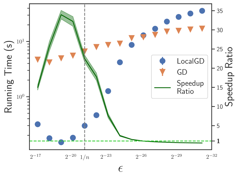
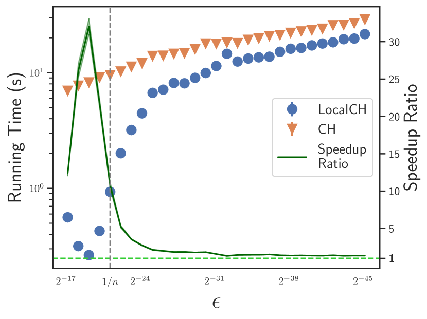
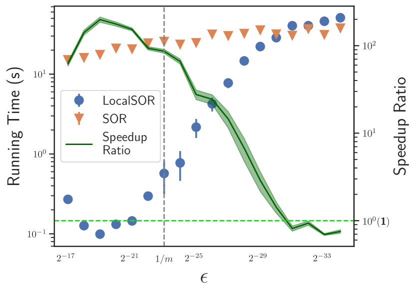

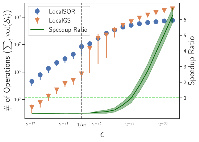
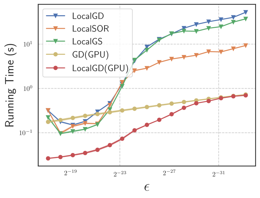
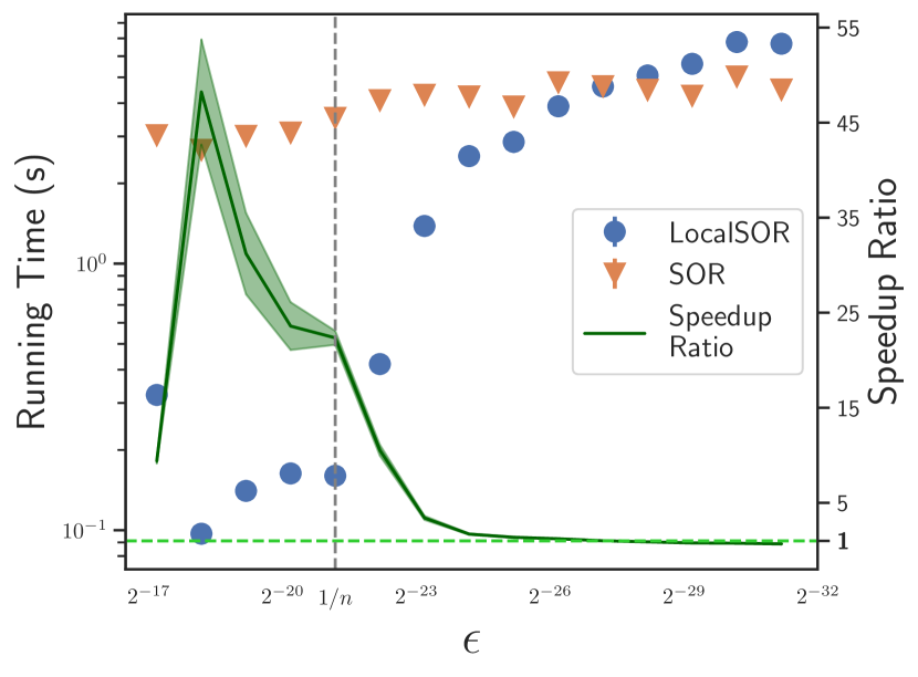
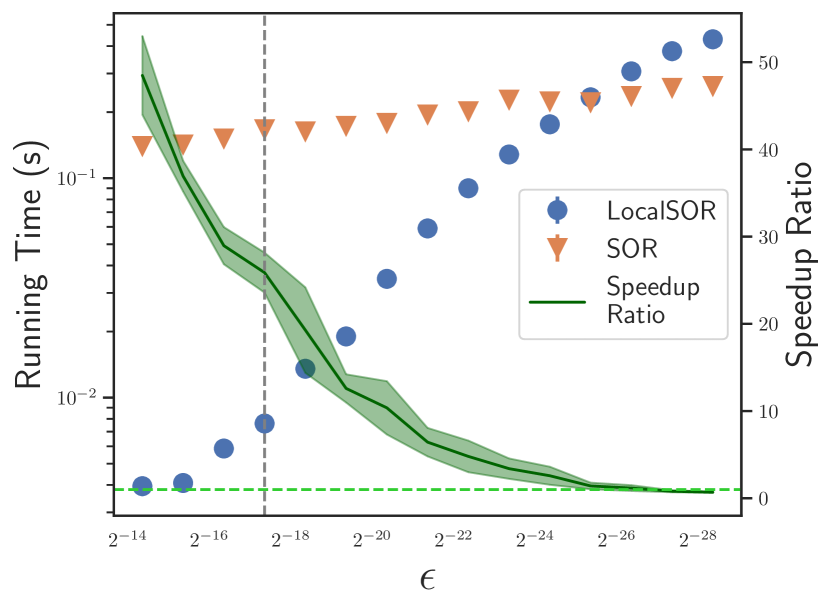
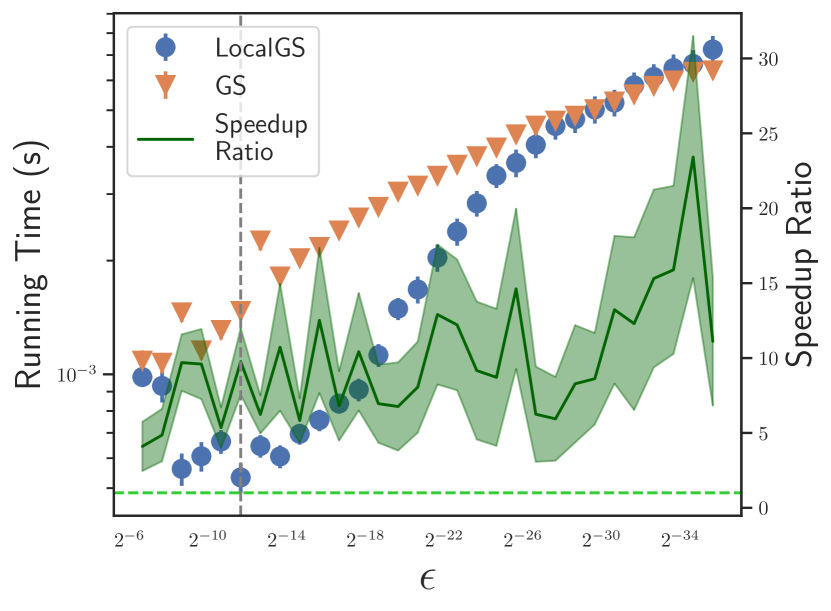
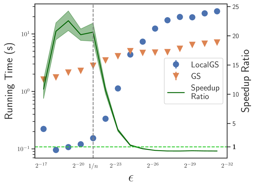
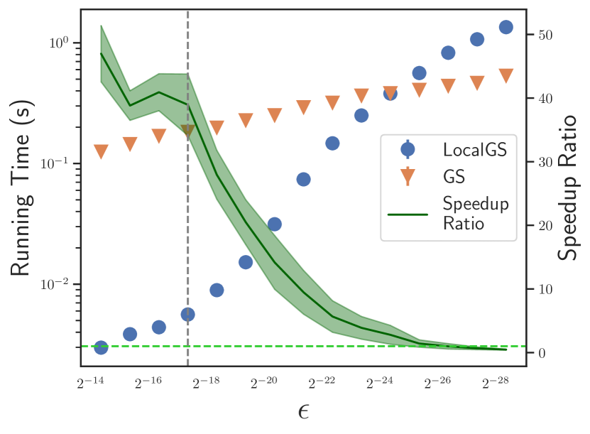
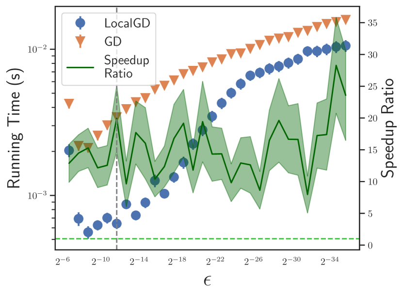
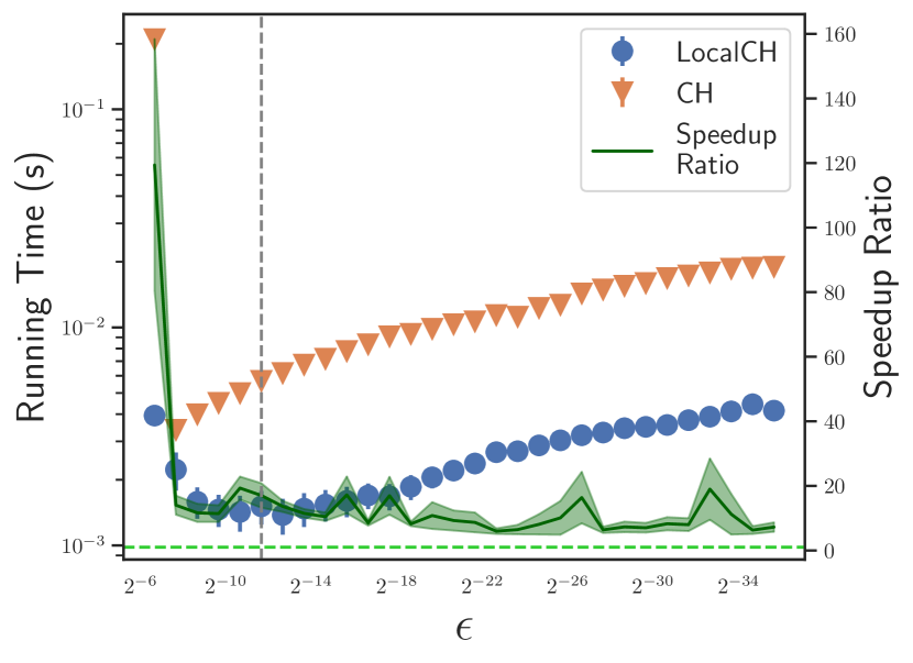
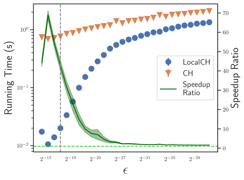
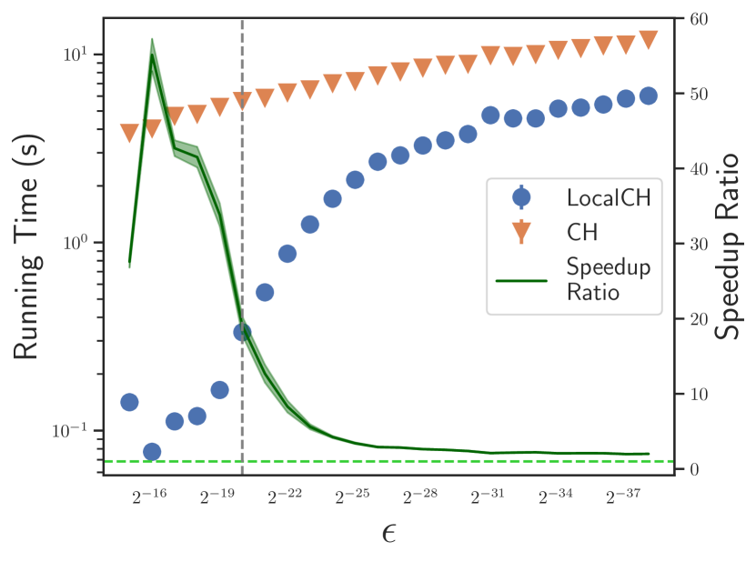
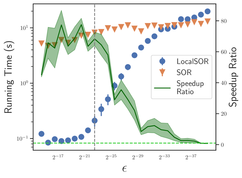
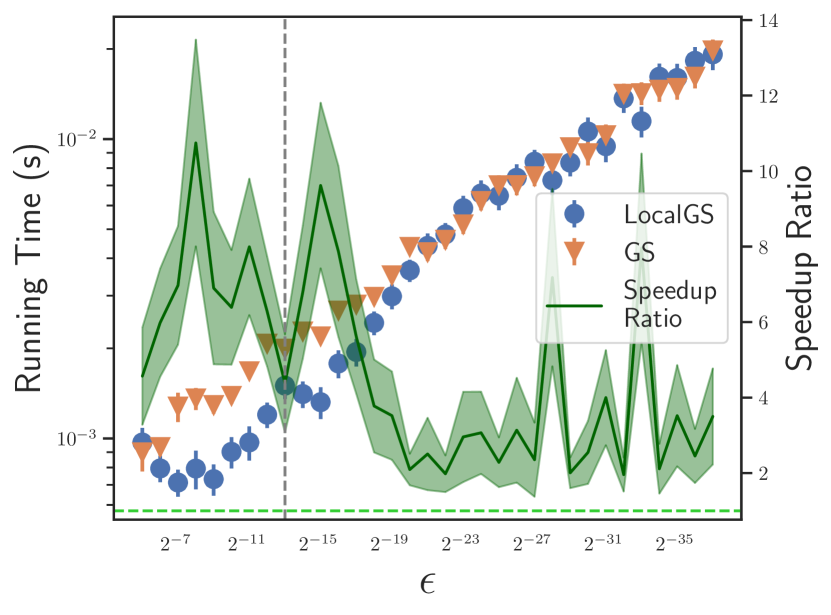
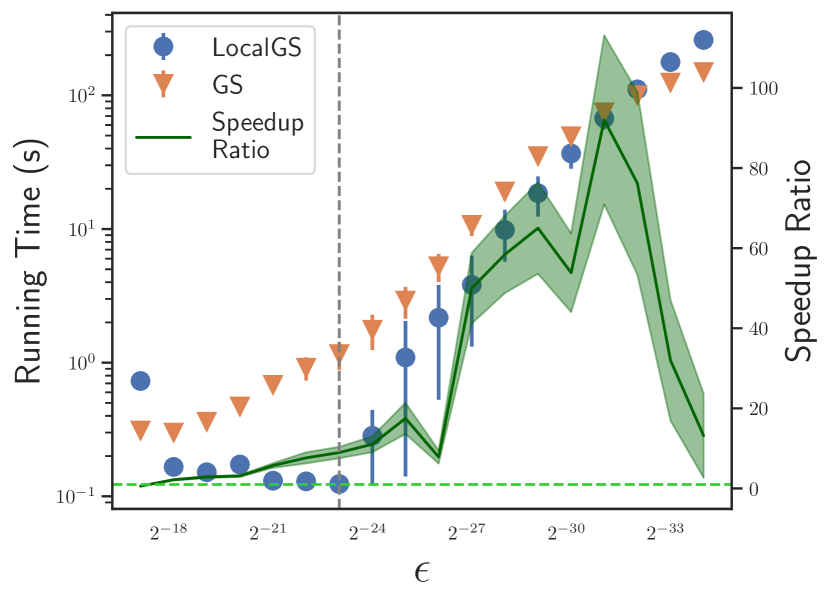
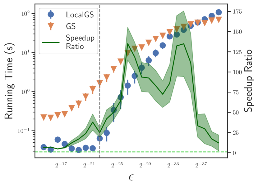
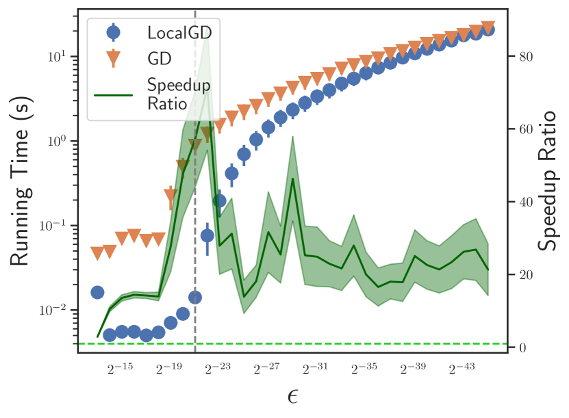
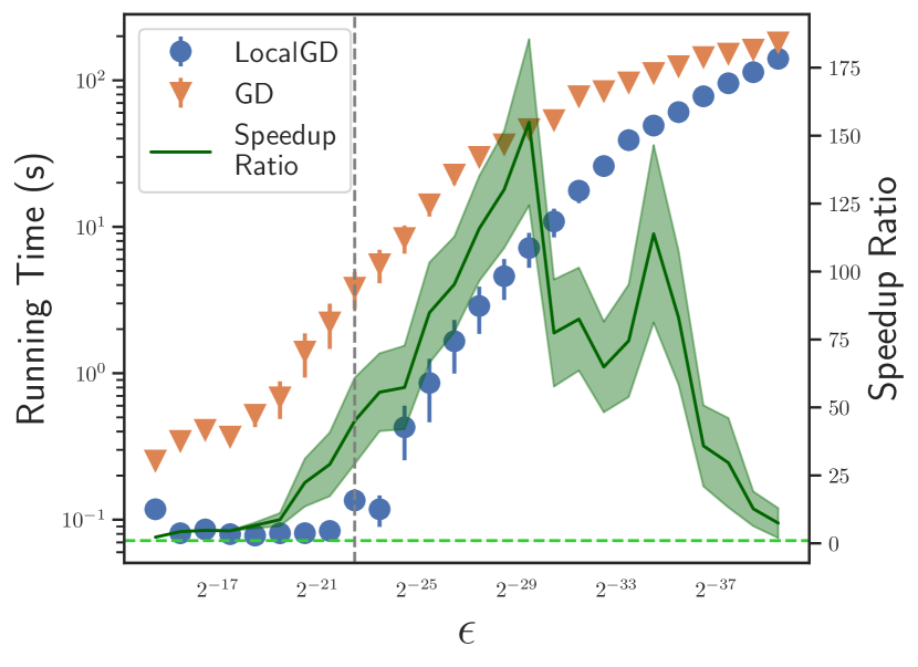
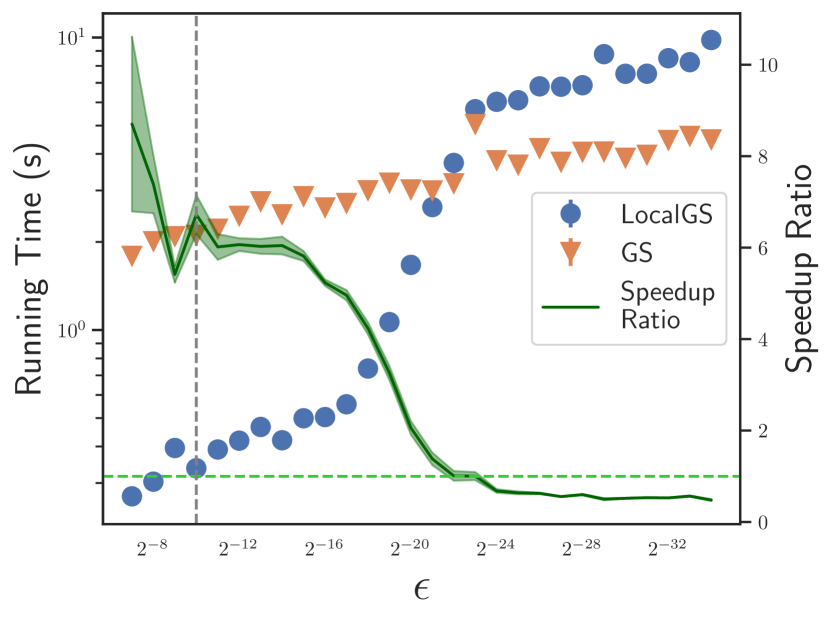
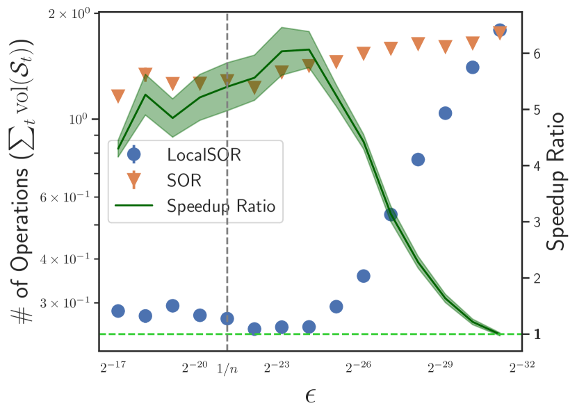
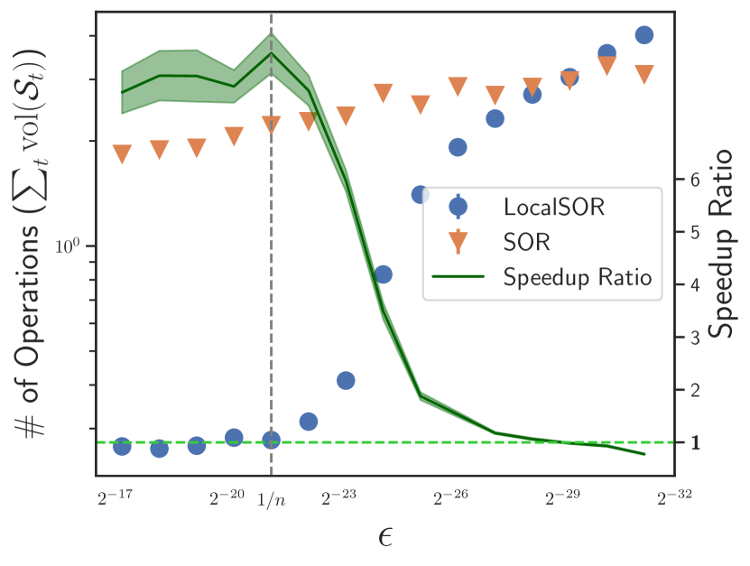
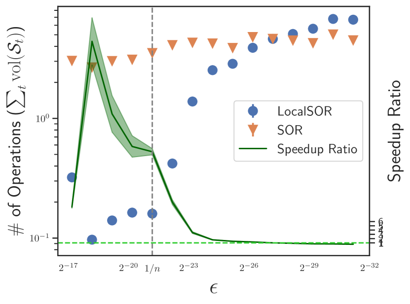
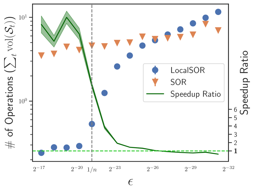
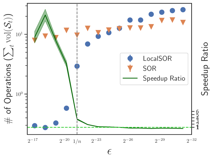
When do local GDE solvers (not) work? The next critical question is when standard solvers can be effectively localized, meaning under which conditions we see speedup over standard solvers. We conduct experiments to determine when local GDE solvers show speedup over their global counterparts for approximating Katz, HK, and PPR on the wiki-talk graph dataset for different values, ranging from lower precision to high precision . As illustrated in Figure 6, when is in the lower range, local methods are much more efficient than the standard counterparts. As expected, the speedup decreases and becomes worse than the standard counterparts when high precision is needed. This indicates the broad applicability of our framework; the required precisions in many real-world graph applications are within a range where our framework is effective.
5.2 Local GDE solvers on GPU-architecture
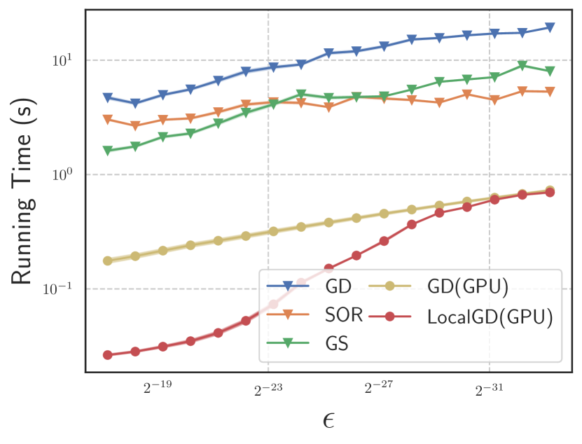
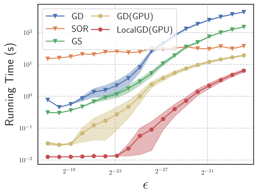
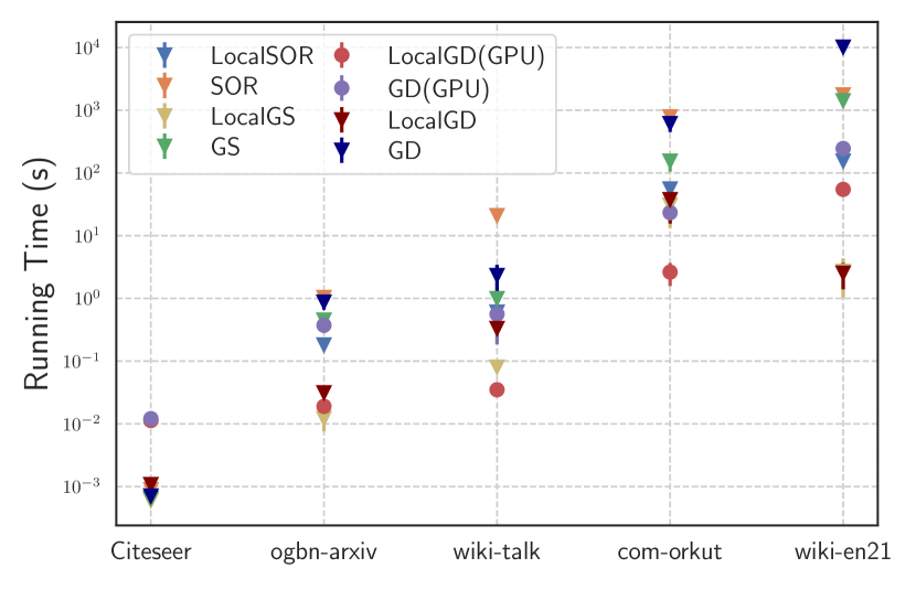
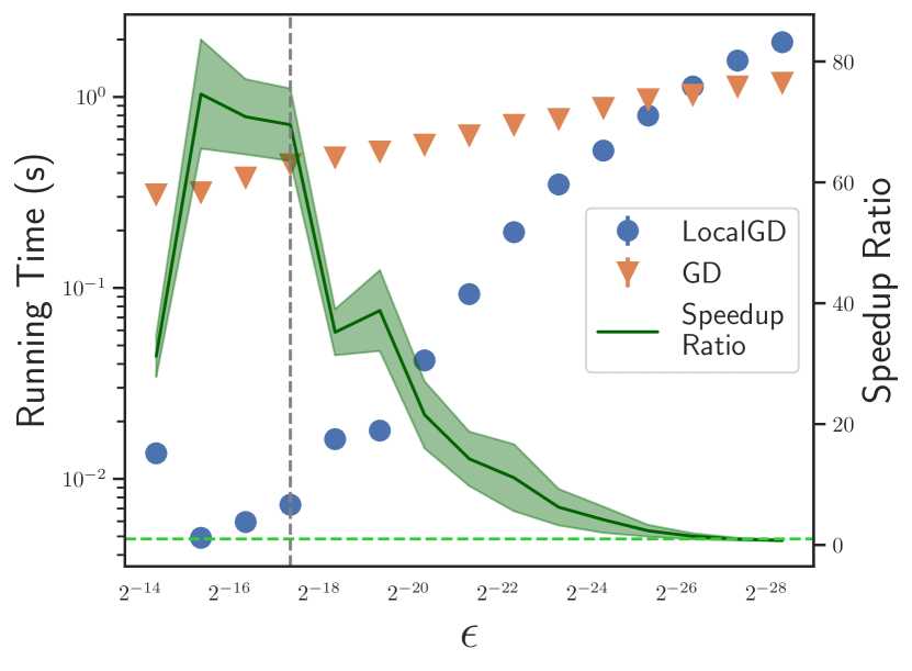
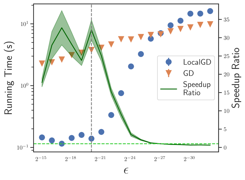
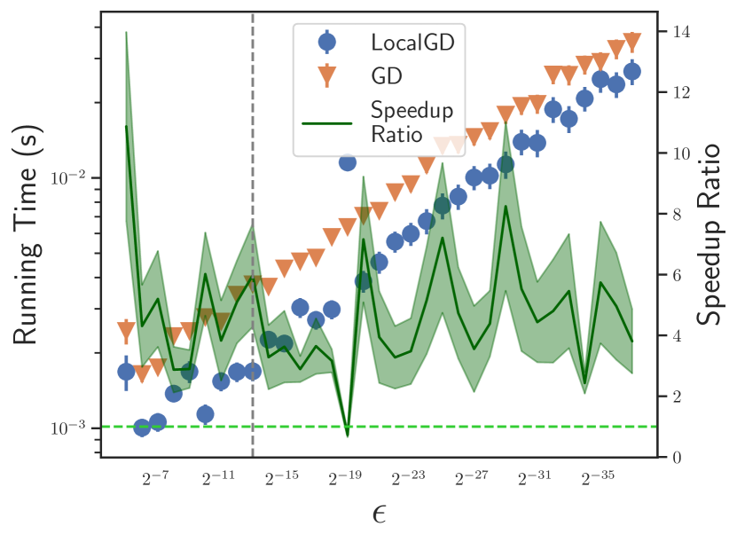
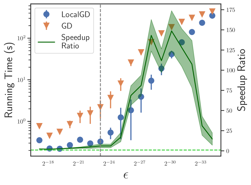
We conducted experiments on the efficiency of the GPU implementation of LocalGD and GD, specifically using LocalGD’s GPU implementation to compare with other methods. Figure 7 presents the running time of global and local solvers as a function of on the wiki-talk dataset. LocalGD is the fastest among a wide range of . This indicates that, when a GPU is available and is within the effective range, LocalGD (GPU) can be much faster than standard GD (GPU) and other methods based on CPUs. We observed similar patterns for computing Katz in Figure 11.
5.3 Dynamic PPR approximating and training GNN models
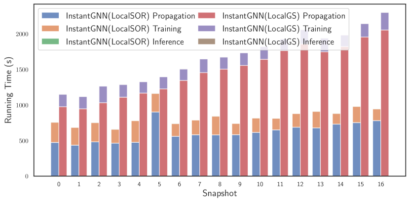
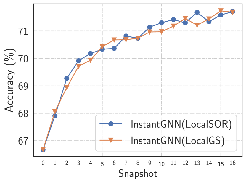
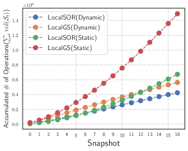
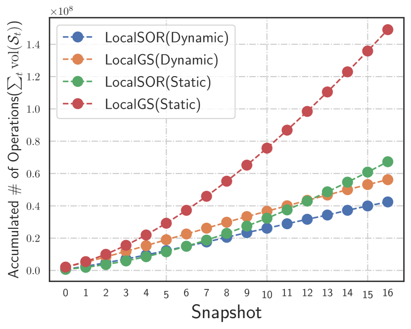
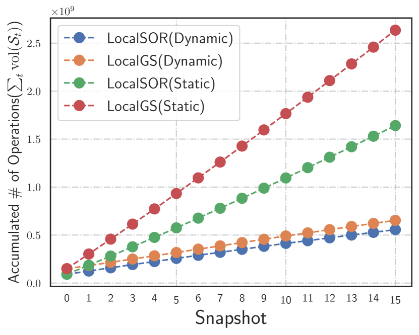
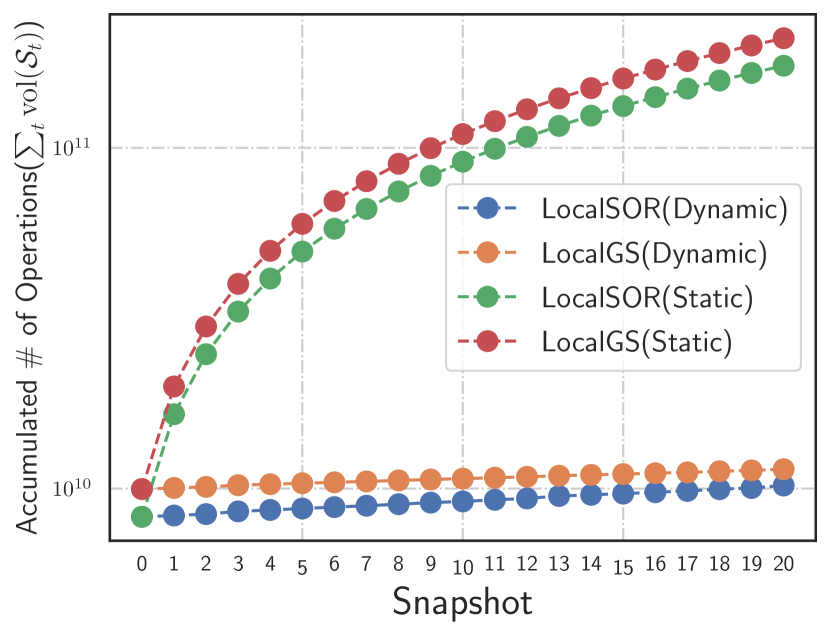
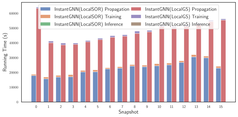
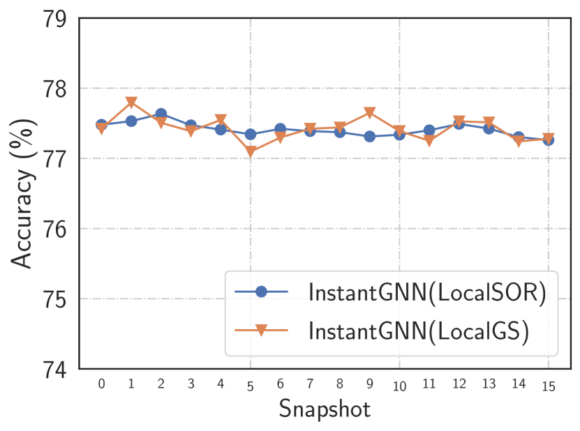
To test the applicability of the proposed local solvers, we apply LocalSOR to GNN propagation and test its efficiency on ogbn-arxiv and ogbn-products. We use the InstantGNN [75] model (essentially APPNP [30]), following the experimental settings in [75]. Specifically, we set , , and to the optimal value for our cases. For ogbn-arxiv, we randomly partition the graph into 16 snapshots (each snapshot with 59,375 edges), where the initial graph contains 17.9% of the edges. With a similar performance on testing accuracy, as illustrated in Figure 8, the InstantGNN model with LocalSOR (Algo. 7) has a significantly shorter training time than its local propagation counterpart (Algo. 6). Figure 9 presents the accumulated operations over these 16 snapshots. The faster local solver is LocalSOR (Dynamic), which dynamically updates for (14) according to Algo. 5 and Algo. 3, whereas LocalSOR (Static) updates all approximate PPR vectors from scratch at the start of each snapshot for (14). We observed a similar pattern for LocalCH, where the number of operations is significantly reduced compared to static ones.
6 Limitations and Conclusion
When is sufficiently small, the speedup is insignificant, and it is unknown whether more efficient local solvers can be designed under this setting. Although we observed acceleration in practice, the accelerated bounds for LocalSOR and LocalCH have not been proven. Another limitation of local solvers is that they inherit the limitations of their standard counterparts. This paper mainly develops local solvers for PPR and Katz, and it remains interesting to consider other types of GDEs.
We propose the local diffusion process, a local iterative algorithm framework based on the locally evolving set process. Our framework is powerful in capturing existing local iterative solvers such as APPR for GDEs. We then demonstrate that standard iterative solvers can be effectively localized, achieving sublinear runtime complexity when monotonicity properties hold in these local solvers. Extensive experiments show that local solvers consistently speed up standard solvers by a hundredfold. We also show that these local solvers could help build faster GNN models [31, 13, 14, 20]. We expect many GNN models to benefit from these local solvers using a local message passing strategy, which we are actively investigating. Several open problems are worth exploring, such as whether these empirically accelerated local solvers admit accelerated sublinear runtime bounds without the monotonicity assumption.
References
- Andersen et al. [2006] Reid Andersen, Fan Chung, and Kevin Lang. Local graph partitioning using PageRank vectors. In 2006 47th Annual IEEE Symposium on Foundations of Computer Science (FOCS’06), pages 475–486. IEEE, 2006.
- Andersen et al. [2007] Reid Andersen, Christian Borgs, Jennifer Chayes, John Hopcraft, Vahab S Mirrokni, and Shang-Hua Teng. Local computation of PageRank contributions. In Algorithms and Models for the Web-Graph: 5th International Workshop, WAW 2007, San Diego, CA, USA, December 11-12, 2007. Proceedings 5, pages 150–165. Springer, 2007.
- Avrachenkov et al. [2007] Konstantin Avrachenkov, Nelly Litvak, Danil Nemirovsky, and Natalia Osipova. Monte carlo methods in PageRank computation: When one iteration is sufficient. SIAM Journal on Numerical Analysis, 45(2):890–904, 2007.
- Avrachenkov et al. [2013] Konstantin Avrachenkov, Paulo Gonçalves, and Marina Sokol. On the choice of kernel and labelled data in semi-supervised learning methods. In Algorithms and Models for the Web Graph: 10th International Workshop, WAW 2013, Cambridge, MA, USA, December 14-15, 2013, Proceedings 10, pages 56–67. Springer, 2013.
- Banerjee and Lofgren [2015] Siddhartha Banerjee and Peter Lofgren. Fast bidirectional probability estimation in markov models. Advances in Neural Information Processing Systems, 28, 2015.
- Benzi and Boito [2020] Michele Benzi and Paola Boito. Matrix functions in network analysis. GAMM-Mitteilungen, 43(3):e202000012, 2020.
- Berkhin [2006] Pavel Berkhin. Bookmark-coloring algorithm for personalized PageRank computing. Internet Mathematics, 3(1):41–62, 2006.
- Bojchevski and Günnemann [2017] Aleksandar Bojchevski and Stephan Günnemann. Deep Gaussian embedding of graphs: Unsupervised inductive learning via ranking. arXiv preprint arXiv:1707.03815, 2017.
- Bojchevski et al. [2019] Aleksandar Bojchevski, Johannes Klicpera, Bryan Perozzi, Martin Blais, Amol Kapoor, Michal Lukasik, and Stephan Günnemann. Is PageRank all you need for scalable graph neural networks. In ACM KDD, MLG Workshop, 2019.
- Bojchevski et al. [2020] Aleksandar Bojchevski, Johannes Gasteiger, Bryan Perozzi, Amol Kapoor, Martin Blais, Benedek Rózemberczki, Michal Lukasik, and Stephan Günnemann. Scaling graph neural networks with approximate PageRank. In Proceedings of the 26th ACM SIGKDD International Conference on Knowledge Discovery & Data Mining, pages 2464–2473, 2020.
- Bonchi et al. [2012] Francesco Bonchi, Pooya Esfandiar, David F Gleich, Chen Greif, and Laks VS Lakshmanan. Fast matrix computations for pairwise and columnwise commute times and Katz scores. Internet Mathematics, 8(1-2):73–112, 2012.
- Borgs et al. [2012] Christian Borgs, Michael Brautbar, Jennifer Chayes, and Shang-Hua Teng. A sublinear time algorithm for PageRank computations. In International Workshop on Algorithms and Models for the Web-Graph, pages 41–53. Springer, 2012.
- Chamberlain et al. [2021a] Ben Chamberlain, James Rowbottom, Maria I Gorinova, Michael Bronstein, Stefan Webb, and Emanuele Rossi. Grand: Graph neural diffusion. In International Conference on Machine Learning, pages 1407–1418. PMLR, 2021a.
- Chamberlain et al. [2021b] Benjamin Chamberlain, James Rowbottom, Davide Eynard, Francesco Di Giovanni, Xiaowen Dong, and Michael Bronstein. Beltrami flow and neural diffusion on graphs. Advances in Neural Information Processing Systems, 34:1594–1609, 2021b.
- Chen et al. [2021] Deli Chen, Yankai Lin, Guangxiang Zhao, Xuancheng Ren, Peng Li, Jie Zhou, and Xu Sun. Topology-imbalance learning for semi-supervised node classification. Advances in Neural Information Processing Systems, 34:29885–29897, 2021.
- Chen et al. [2020a] Ming Chen, Zhewei Wei, Bolin Ding, Yaliang Li, Ye Yuan, Xiaoyong Du, and Ji-Rong Wen. Scalable graph neural networks via bidirectional propagation. Advances in neural information processing systems, 33:14556–14566, 2020a.
- Chen et al. [2020b] Ming Chen, Zhewei Wei, Zengfeng Huang, Bolin Ding, and Yaliang Li. Simple and deep graph convolutional networks. In International conference on machine learning, pages 1725–1735. PMLR, 2020b.
- Chen et al. [2023] Zhen Chen, Xingzhi Guo, Baojian Zhou, Deqing Yang, and Steven Skiena. Accelerating personalized PageRank vector computation. In Proceedings of the 29th ACM SIGKDD Conference on Knowledge Discovery and Data Mining, pages 262–273, 2023.
- Chien et al. [2021] Eli Chien, Jianhao Peng, Pan Li, and Olgica Milenkovic. Adaptive universal generalized PageRank graph neural network. In International Conference on Learning Representations (ICLR), 2021.
- Choi et al. [2023] Jeongwhan Choi, Seoyoung Hong, Noseong Park, and Sung-Bae Cho. GREAD: Graph neural reaction-diffusion networks. In International Conference on Machine Learning, pages 5722–5747. PMLR, 2023.
- Chung [2007] Fan Chung. The heat kernel as the PageRank of a graph. Proceedings of the National Academy of Sciences, 104(50):19735–19740, 2007.
- Clark and Del Maestro [2018] Timothy BP Clark and Adrian Del Maestro. Moments of the inverse participation ratio for the laplacian on finite regular graphs. Journal of Physics A: Mathematical and Theoretical, 51(49):495003, 2018.
- Deng et al. [2023] Haoran Deng, Yang Yang, Jiahe Li, Haoyang Cai, Shiliang Pu, and Weihao Jiang. Accelerating dynamic network embedding with billions of parameter updates to milliseconds. In Proceedings of the 29th ACM SIGKDD Conference on Knowledge Discovery and Data Mining, pages 414–425, 2023.
- d’Aspremont et al. [2021] Alexandre d’Aspremont, Damien Scieur, Adrien Taylor, et al. Acceleration methods. Foundations and Trends® in Optimization, 5(1-2):1–245, 2021.
- Epasto et al. [2022] Alessandro Epasto, Vahab Mirrokni, Bryan Perozzi, Anton Tsitsulin, and Peilin Zhong. Differentially private graph learning via sensitivity-bounded personalized PageRank. Advances in Neural Information Processing Systems, 35:22617–22627, 2022.
- Farkas et al. [2001] Illés J Farkas, Imre Derényi, Albert-László Barabási, and Tamas Vicsek. Spectra of “real-world” graphs: Beyond the semicircle law. Physical Review E, 64(2):026704, 2001.
- Fountoulakis and Yang [2022] Kimon Fountoulakis and Shenghao Yang. Open problem: Running time complexity of accelerated -regularized pagerank. In Conference on Learning Theory, pages 5630–5632. PMLR, 2022.
- Fu et al. [2020] Dongqi Fu, Dawei Zhou, and Jingrui He. Local motif clustering on time-evolving graphs. In Proceedings of the 26th ACM SIGKDD International conference on knowledge discovery & data mining, pages 390–400, 2020.
- Fu et al. [2024] Dongqi Fu, Zhigang Hua, Yan Xie, Jin Fang, Si Zhang, Kaan Sancak, Hao Wu, Andrey Malevich, Jingrui He, and Bo Long. VCR-graphormer: A mini-batch graph transformer via virtual connections. In The Twelfth International Conference on Learning Representations, 2024. URL https://openreview.net/forum?id=SUUrkC3STJ.
- Gasteiger et al. [2019a] Johannes Gasteiger, Aleksandar Bojchevski, and Stephan Günnemann. Predict then propagate: Graph neural networks meet personalized PageRank. In International Conference on Learning Representations (ICLR), 2019a.
- Gasteiger et al. [2019b] Johannes Gasteiger, Stefan Weißenberger, and Stephan Günnemann. Diffusion improves graph learning. Advances in neural information processing systems, 32, 2019b.
- Gleich [2015] David F Gleich. PageRank beyond the web. siam REVIEW, 57(3):321–363, 2015.
- Gleich et al. [2015] David F Gleich, Kyle Kloster, and Huda Nassar. Localization in seeded PageRank. arXiv preprint arXiv:1509.00016, 2015.
- Golub and Van Loan [2013] Gene H Golub and Charles F Van Loan. Matrix computations. JHU press, 2013.
- Guhr et al. [1998] Thomas Guhr, Axel Müller-Groeling, and Hans A Weidenmüller. Random-matrix theories in quantum physics: common concepts. Physics Reports, 299(4-6):189–425, 1998.
- Guo et al. [2017] Wentian Guo, Yuchen Li, Mo Sha, and Kian-Lee Tan. Parallel personalized PageRank on dynamic graphs. Proceedings of the VLDB Endowment, 11(1):93–106, 2017.
- Guo et al. [2021] Xingzhi Guo, Baojian Zhou, and Steven Skiena. Subset node representation learning over large dynamic graphs. In Proceedings of the 27th ACM SIGKDD Conference on Knowledge Discovery & Data Mining, pages 516–526, 2021.
- Guo et al. [2022] Xingzhi Guo, Baojian Zhou, and Steven Skiena. Subset node anomaly tracking over large dynamic graphs. In Proceedings of the 28th ACM SIGKDD Conference on Knowledge Discovery and Data Mining, pages 475–485, 2022.
- Gutknecht and Röllin [2002] Martin H Gutknecht and Stefan Röllin. The chebyshev iteration revisited. Parallel Computing, 28(2):263–283, 2002.
- Hamilton et al. [2017] Will Hamilton, Zhitao Ying, and Jure Leskovec. Inductive representation learning on large graphs. Advances in neural information processing systems, 30, 2017.
- Haveliwala [2002] Taher H Haveliwala. Topic-sensitive PageRank. In Proceedings of the 11th international conference on World Wide Web, pages 517–526, 2002.
- Hu et al. [2021] Weihua Hu, Matthias Fey, Hongyu Ren, Maho Nakata, Yuxiao Dong, and Jure Leskovec. Ogb-lsc: A large-scale challenge for machine learning on graphs. arXiv preprint arXiv:2103.09430, 2021.
- Jain et al. [2014] Prateek Jain, Ambuj Tewari, and Purushottam Kar. On iterative hard thresholding methods for high-dimensional m-estimation. Advances in neural information processing systems, 27, 2014.
- Jeh and Widom [2003] Glen Jeh and Jennifer Widom. Scaling personalized web search. In Proceedings of the 12th international conference on World Wide Web, pages 271–279, 2003.
- Jure [2014] Leskovec Jure. Snap datasets: Stanford large network dataset collection. Retrieved December 2021 from http://snap. stanford. edu/data, 2014.
- Katz [1953] Leo Katz. A new status index derived from sociometric analysis. Psychometrika, 18(1):39–43, 1953.
- Kazemi et al. [2020] Seyed Mehran Kazemi, Rishab Goel, Kshitij Jain, Ivan Kobyzev, Akshay Sethi, Peter Forsyth, and Pascal Poupart. Representation learning for dynamic graphs: a survey. The Journal of Machine Learning Research, 21(1):2648–2720, 2020.
- Kloster and Gleich [2013] Kyle Kloster and David F Gleich. A nearly-sublinear method for approximating a column of the matrix exponential for matrices from large, sparse networks. In Algorithms and Models for the Web Graph: 10th International Workshop, WAW 2013, Cambridge, MA, USA, December 14-15, 2013, Proceedings 10, pages 68–79. Springer, 2013.
- Kloster and Gleich [2014] Kyle Kloster and David F Gleich. Heat kernel based community detection. In Proceedings of the 20th ACM SIGKDD international conference on Knowledge discovery and data mining, pages 1386–1395, 2014.
- Kloumann et al. [2017] Isabel M Kloumann, Johan Ugander, and Jon Kleinberg. Block models and personalized PageRank. Proceedings of the National Academy of Sciences, 114(1):33–38, 2017.
- Li et al. [2019] Pan Li, I Chien, and Olgica Milenkovic. Optimizing generalized pagerank methods for seed-expansion community detection. Advances in Neural Information Processing Systems, 32, 2019.
- Li et al. [2023] Yiming Li, Yanyan Shen, Lei Chen, and Mingxuan Yuan. Zebra: When temporal graph neural networks meet temporal personalized PageRank. Proceedings of the VLDB Endowment, 16(6):1332–1345, 2023.
- Lofgren et al. [2015] Peter Lofgren, Siddhartha Banerjee, and Ashish Goel. Bidirectional PageRank estimation: From average-case to worst-case. In Algorithms and Models for the Web Graph: 12th International Workshop, WAW 2015, Eindhoven, The Netherlands, December 10-11, 2015, Proceedings 12, pages 164–176. Springer, 2015.
- Martin et al. [2014] Travis Martin, Xiao Zhang, and Mark EJ Newman. Localization and centrality in networks. Physical review E, 90(5):052808, 2014.
- McSherry [2005] Frank McSherry. A uniform approach to accelerated PageRank computation. In Proceedings of the 14th international conference on World Wide Web, pages 575–582, 2005.
- Mo and Luo [2021] Dingheng Mo and Siqiang Luo. Agenda: Robust personalized PageRanks in evolving graphs. In Proceedings of the 30th ACM International Conference on Information & Knowledge Management, pages 1315–1324, 2021.
- Moler and Van Loan [2003] Cleve Moler and Charles Van Loan. Nineteen dubious ways to compute the exponential of a matrix, twenty-five years later. SIAM review, 45(1):3–49, 2003.
- Morris and Peres [2003] Ben Morris and Yuval Peres. Evolving sets and mixing. In Proceedings of the Thirty-Fifth Annual ACM Symposium on Theory of Computing (STOC), page 279–286, New York, NY, USA, 2003. Association for Computing Machinery.
- Nassar et al. [2015] Huda Nassar, Kyle Kloster, and David F Gleich. Strong localization in personalized PageRank vectors. In Algorithms and Models for the Web Graph: 12th International Workshop, WAW 2015, Eindhoven, The Netherlands, December 10-11, 2015, Proceedings 12, pages 190–202. Springer, 2015.
- Nassar et al. [2017] Huda Nassar, Kyle Kloster, and David F Gleich. Localization in seeded PageRank. Internet Mathematics, 2017.
- Orecchia et al. [2012] Lorenzo Orecchia, Sushant Sachdeva, and Nisheeth K Vishnoi. Approximating the exponential, the lanczos method and an -time spectral algorithm for balanced separator. In Proceedings of the forty-fourth annual ACM symposium on Theory of computing, pages 1141–1160, 2012.
- Page et al. [1998] Lawrence Page, Sergey Brin, Rajeev Motwani, and Terry Winograd. The PageRank Citation Ranking: Bringing Order to the Web. Technical report, Stanford Digital Library Technologies Project, 1998.
- Postăvaru et al. [2020] Ştefan Postăvaru, Anton Tsitsulin, Filipe Miguel Gonçalves de Almeida, Yingtao Tian, Silvio Lattanzi, and Bryan Perozzi. Instantembedding: Efficient local node representations. arXiv preprint arXiv:2010.06992, 2020.
- Sarkar et al. [2008] Purnamrita Sarkar, Andrew W Moore, and Amit Prakash. Fast incremental proximity search in large graphs. In Proceedings of the 25th international conference on Machine learning, pages 896–903, 2008.
- Scholtes [2017] Ingo Scholtes. When is a network a network? multi-order graphical model selection in pathways and temporal networks. In Proceedings of the 23rd ACM SIGKDD international conference on knowledge discovery and data mining, pages 1037–1046, 2017.
- Shi et al. [2019] Jieming Shi, Renchi Yang, Tianyuan Jin, Xiaokui Xiao, and Yin Yang. Realtime top-k personalized PageRank over large graphs on gpus. Proceedings of the VLDB Endowment, 13(1):15–28, 2019.
- Tsitsulin et al. [2021] Anton Tsitsulin, Marina Munkhoeva, Davide Mottin, Panagiotis Karras, Ivan Oseledets, and Emmanuel Müller. FREDE: anytime graph embeddings. Proceedings of the VLDB Endowment, 14(6):1102–1110, 2021.
- Wang et al. [2021] Hanzhi Wang, Mingguo He, Zhewei Wei, Sibo Wang, Ye Yuan, Xiaoyong Du, and Ji-Rong Wen. Approximate graph propagation. In Proceedings of the 27th ACM SIGKDD Conference on Knowledge Discovery & Data Mining, pages 1686–1696, 2021.
- Wu et al. [2019] Felix Wu, Amauri Souza, Tianyi Zhang, Christopher Fifty, Tao Yu, and Kilian Weinberger. Simplifying graph convolutional networks. In International conference on machine learning, pages 6861–6871. PMLR, 2019.
- Wu et al. [2021] Hao Wu, Junhao Gan, Zhewei Wei, and Rui Zhang. Unifying the global and local approaches: an efficient power iteration with forward push. In Proceedings of the 2021 International Conference on Management of Data, pages 1996–2008, 2021.
- Yin et al. [2017] Hao Yin, Austin R Benson, Jure Leskovec, and David F Gleich. Local higher-order graph clustering. In Proceedings of the 23rd ACM SIGKDD international conference on knowledge discovery and data mining, pages 555–564, 2017.
- Zeng et al. [2021] Hanqing Zeng, Muhan Zhang, Yinglong Xia, Ajitesh Srivastava, Andrey Malevich, Rajgopal Kannan, Viktor Prasanna, Long Jin, and Ren Chen. Decoupling the depth and scope of graph neural networks. Advances in Neural Information Processing Systems, 34:19665–19679, 2021.
- Zhang et al. [2016] Hongyang Zhang, Peter Lofgren, and Ashish Goel. Approximate personalized PageRank on dynamic graphs. In Proceedings of the 22nd ACM SIGKDD international conference on knowledge discovery and data mining, pages 1315–1324, 2016.
- Zhao et al. [2021] Jialin Zhao, Yuxiao Dong, Ming Ding, Evgeny Kharlamov, and Jie Tang. Adaptive diffusion in graph neural networks. Advances in neural information processing systems, 34:23321–23333, 2021.
- Zheng et al. [2022] Yanping Zheng, Hanzhi Wang, Zhewei Wei, Jiajun Liu, and Sibo Wang. Instant graph neural networks for dynamic graphs. In Proceedings of the 28th ACM SIGKDD conference on knowledge discovery and data mining, pages 2605–2615, 2022.
- Zhou et al. [2023] Baojian Zhou, Yifan Sun, and Reza Babanezhad Harikandeh. Fast online node labeling for very large graphs. In International Conference on Machine Learning, pages 42658–42697. PMLR, 2023.
- Zhou et al. [2024] Baojian Zhou, Yifan Sun, Reza Babanezhad Harikandeh, Xingzhi Guo, Deqing Yang, and Yanghua Xiao. Iterative methods via locally evolving set process. arXiv preprint arXiv:2410.15020, 2024.
- Zhou et al. [2003] Dengyong Zhou, Olivier Bousquet, Thomas Lal, Jason Weston, and Bernhard Schölkopf. Learning with local and global consistency. Advances in neural information processing systems, 16, 2003.
- Zhu et al. [2021] Qi Zhu, Natalia Ponomareva, Jiawei Han, and Bryan Perozzi. Shift-robust GNNs: Overcoming the limitations of localized graph training data. Advances in Neural Information Processing Systems, 34:27965–27977, 2021.
- Zhu et al. [2003] Xiaojin Zhu, Zoubin Ghahramani, and John D Lafferty. Semi-supervised learning using Gaussian fields and harmonic functions. In Proceedings of the 20th International conference on Machine learning (ICML-03), pages 912–919, 2003.
- Zhu et al. [2013] Zeyuan Allen Zhu, Silvio Lattanzi, and Vahab Mirrokni. A local algorithm for finding well-connected clusters. In International Conference on Machine Learning, pages 396–404. PMLR, 2013.
Appendix A Related Work
Disclaimer: The local diffusion process introduced in this paper shares a similar conceptual foundation with our concurrent work [77], where we propose the locally evolving set process. However, these two approaches address distinct problems. In this work, our focus is on investigating a different class of equations and exploring whether the local diffusion process can accelerate the training of Graph Neural Networks (GNNs).
Graph diffusion equations (GDEs) and localization. Graph diffusion vectors can either be exactly represented as a linear system or be approximations of an underlying linear system. The general form defined in Equation (1) has appeared in various literature [49, 51] (see more examples in [68]) or can be found in the survey works of [32]. The locality and localization properties of the diffusion vector , including the PPR vector, have been explored in [64, 1, 59, 33, 60]. Inspired by methods for measuring the dynamic localization of quantum chaos [35, 22], which are also used for analyzing graph eigenfunctions [11, 26, 54], we use the inverse participation ratio to measure the localization ability of . However, there is a lack of a local framework for solving GDEs efficiently.
Standard solvers for GDEs. The computation of a graph diffusion equation approximates the exponential of a propagation matrix, either through an inherently Neumann series or as an analytic system of linear equations. Well-established iterative methods, such as those approximating via the Neumann series or Padé approximations, exist (see more details in the surveys [57, 6, 61] and [34]). Each iteration requires computing the matrix-vector dot product, requiring operations for all the above methods. This is the computation we aim to avoid.
Local methods for GDEs. The most well-known local solver for solving PPR was initially proposed in [1] for local clustering. PPR, as a fundamental tool for graph learning, has been applied to many core problems, including graph neural networks [10, 17, 69, 15], graph diffusion [31, 74], and its generalizations [51, 19] for GNNs or clustering [50, 71]. Many variants have been proposed for solving such equations in different forms using local methods that couple local methods with Monte Carlo sampling strategies, achieving sublinear time [5, 53]. The work of [55] attempts to accelerate PPR computation via the Gauss-Southwell method, but it does not work well in practice [48]. A notable finding from [70] is that the local computation of PPR is equivalent to power iteration when the precision is high. There are also works on temporal PPR vector computation [66, 36, 56, 52], and our work can be immediately applied to these. Some local variants of APPR have been proposed for Katz and HK [11, 49]. However, these local solvers are sequential and lack the ability to be easily implemented on GPUs. Our local framework addresses this challenge.
PPR on dynamic graphs. Ranking on dynamic graphs has many applications [65], including motif clustering [71, 28], embedding on large-scale graphs [63, 23, 37, 38, 76, 18], and designing graph neural networks [75, 72]. The local computation via forward push (a.k.a. APPR algorithm [1]) or reverse push (a.k.a. reverse APPR [2]) is widely used in GNN propagation and bidirectional propagation algorithms [16, 29]. Our framework helps to design more efficient dynamic GNNs.
Appendix B Missing Proofs
B.1 Notations
We list all notations used in our proofs here.
-
•
: The indicator vector where the -th entry is 1, and 0 otherwise.
-
•
: Set of neighbors of node .
-
•
: The degree of node .
-
•
: The underlying graph with the set of nodes and set of edges .
-
•
: Adjacency matrix of .
-
•
: Degree matrix of when is undirected.
-
•
: Personalized PPR matrix, defined as .
-
•
: Damping factor for the PPR equation.
-
•
: Parameter for the Katz equation.
-
•
: The error tolerance.
-
•
: The stop condition for local solvers of PPR.
-
•
: The stop condition for local solvers of Katz.
B.2 Formulation of PPR and Katz
In this section, we restate all theorems and present all missing proofs. We first restate the two target linear systems we aim to solve, as introduced in Section 3. Recall PPR is defined as . It can be equivalently written as
| (15) |
where and . Hence, . The Katz centrality can be written as
| (16) |
where . Then . 444We will arbitrarily write and as when the context is clear.
Proposition B.1 ([4, 53]).
Let be an undirected graph and and be two vertices in . Denote as the PPR vector of a source node . Then
Proof.
We directly follow the proof strategy in [53] for completeness. For path in , we denote its length as (here ), and define its reverse path to be note that . Moreover, we know that a random walk starting from traverses path with probability , and thus, it is easy to see that we have
Now let denote the paths in starting at and terminating at . Then, we can re-write as:
∎
We adopt the typical implementation of APPR as presented in Algo. 1.
B.3 Missing proofs of LocalSOR
Theorem 3.2 (Properties of local diffusion process via LocalSOR).
Let where and if ; 0 otherwise. Define maximal value . Assume that is nonnegative and , are such that , given the updates of (6), then the local diffusion process of with has the following properties
-
1.
Nonnegativity. for all and with .
-
2.
Monotonicity property. .
If the local diffusion process converges (i.e., ), then is bounded by
Proof.
At each step and where , recall LocalSOR for solving has the following updates
Since we define as , where for all , and using , we continue to have the updates of as follows
By using induction, we show the nonnegativity of . First of all, by our assumption. Let us assume , then the above equation gives since and by our assumption. Since we assume and , the above equation can be written as . By taking on both sides, we have
To make an effective reduction, should be such that for all . Summing over of the above equation, we then have the following
| (17) |
Note that we defined and for all . The inequality of (17) leads to the following bound
To further simply the above upper bound, since each term during the updates, it follows that . If there exists such that , then we can obtain an upper bound of as
which leads to
∎
Theorem 3.3 (Sublinear runtime bound of LocalSOR for PPR).
Let . Given an undirected graph and a target source node with , and provided , the run time of LocalSOR in Equ. (6) for solving with the stop condition and initials and is bounded as the following
| (18) |
where . The estimate satisfies .
Proof.
Recall be the set of active nodes processed in iteration. For convenience, we denote . By LocalSOR defined in (6) for solving
We have the following online iteration updates for each active node (recall ).
Note for each active node , we have . The total operations for LocSOR is
where the last equality follows from and . Next, we focus on the proof of our newly derived bound . To check the upper bound of , from Theorem 3.2 by noticing and , this leads to the following
Next, we try to give a lower bound of . Note that after the last iteration , for each nonzero residual , there is at least one possible update that happened at node : 1) Node has a neighbor , which was active. This neighbor pushed some residual to where the time . Hence, for all , we have
where the first equality is due to the nonnegativity of guaranteeing by Theorem 3.2 and the second inequality is due to the fact that was active residuals before the push operation. Applying the above lower bound of , we obtain
where and . Combine the above inequality and the upper bound , we obtain our new local diffusion-based bounds. The rest is to show a lower bound of . By using the active node condition, for , we have
| (19) |
We continue to have
where the first inequality follows from the fact that for , due to the monotonicity property of . The last inequality is from (19). Combining these, we finish the proof of the sublinear runtime bound. The rest is to prove the estimation quality. Note directly implies by using Proposition B.1 and the corresponding stop condition. ∎
Remark B.2.
The above theorem shares the proof strategy we provided in [77]. Here, we use a slightly different formulation of the linear system.
Corollary 3.4 (Runtime bound of LocalSOR for Katz).
Let and . Given an undirected graph and a target source node with , and provided , the run time of LocalSOR in Equ. (6) for solving with the stop condition and initials and is bounded as the following
| (20) |
The estimate satisfies .
Proof.
The linear system using LocalSOR updates can be written as
where . The updates of can be simplified as the following
The proof of nonnegativity of follows the similar induction as in previous theorem by noticing the spectral radius of is . Hence, we have
Move the negative term to left and take -norm on both sides, we have
It leads to the following
Since each , , we continue have
Finally, the above inequality gives the following upper runtime bound as
By letting and with , we apply Theorem 3.2, to obtain the local diffusion-based bound as
Using the similar technique provided in the previous case, and letting we can have
To check the estimate equality, we have
Let This leads to
∎
B.4 Missing proofs of LocalGD
Theorem 3.5 (Properties of local diffusion process via LocalGD).
Let where and if ; 0 otherwise. Define maximal value . Assume that and , are such that , given the updates of (10), then the local diffusion process of has the following properties
-
1.
Nonnegativity. for all .
-
2.
Monotonicity property.
If the local diffusion process converges (i.e., ), then is bounded by
Proof.
At each step , recall LocalGD for solving has the following updates
Since , we continue to have the updates of as the following
By using induction, we show the nonnegativity of . First of all, by our assumption. Let us assume . Then, the above equation gives since and by our assumption. The above equation can be written as
Taking on both sides, we have
To make an effective reduction, should be such that for all . For this, we then have the following
| (21) |
where note we defined and assumed . Apply (21) from to , it leads to the following bound
Note each of the term during the updates, then . To check the upper bound of , we have
which leads to
∎
Corollary 3.6 (Convergence of LocalGD for PPR and Katz).
Let and . Use LocalGD to approximate PPR or Katz by using iterative procedure (10). Denote and as the total number of operations needed by using LocalGD, they can then be bounded by
| (22) |
for a stop condition . For solving Katz, then the toal runtime is bounded by
| (23) |
for a stop condition . The estimate equality is the same as of LocalSOR.
Proof.
We first show graph-independent bound for PPR computation. Since , then rearrange it to555To simplify the proof, here represents .
Note that entries in are nonnegative. It leads to
where note , then we have
At step , LocalGD accesses the indices in . By the active node condition , we have
Then the total run time of LocalGD is
where the last inequality is due to . Therefore, the total run time is . Follow the similar technique, we have sublinear runtime bound for Katz, i.e., . Next, we show the local diffusion bound for PPR. Recall LocalGD has the initial and the following updates
Since and , by applying Theorem 3.5, we have the upper bound of
Note that each nonzero has at least part of the magnitude from the push operation of an active node. This means each nonzero of satisfies
where . Hence, we have
where . To see the additive error, note that . It has the following equality
To estimate the bound , we need to know . Specifically, the -th entry of the above is
By Proposition B.1, we know , then we continue to have
where the first inequality is due to , and the last equality follows from . Combining all inequalities for , we have the estimate . We omit the proof of the sublinear runtime bound of LocalGD for Katz, as it largely follows the proof technique in Corollary 3.4. For the two lower bounds of , i.e., , it directly follows from the monotonicity and nonnegativity properties stated in Theorem 3.2 and Theorem 3.5. ∎
Remark B.3.
The part of the theorem shares the similar proof strategy we provided in [77]. Here, we use a slightly different formulation of the linear system.
B.5 Implementation Details
-
•
Chebyshev for PPR. Let and . Then . The eigenvalue of is in range . So, we let and .
-
1.
.
-
2.
When , we have
-
3.
When , we have
For LocalCH, we change the update to the update . The final estimate .
-
1.
-
•
Chebyshev for Katz. We want to solve . We assume . Then, the updates of LocalCH for Katz centrality are
-
1.
When , . To obtain an initial value , we have 666This is because .
-
2.
When , we have
-
3.
When , it updates the estimate-residual pair as
For LocalCH, we change the update to the update . The final estimate is then .
-
1.
B.6 FIFO-Queue and Priority-Queue
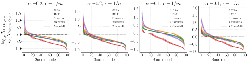
We examine the different data structures of local methods and explore two types: the First-In-First-Out (FIFO) Queue, which requires constant time for updates, and the Priority Queue, which is used to implement the Gauss-Southwell algorithm as described in [48, 7]. We test the number of operations needed using these two data structures on five small graphs, including Cora , Cora-ML , Citeseer , Dblp , and Pubmed as used in [8] and downloaded from https://github.com/abojchevski/graph2gauss.
Figure 10 presents the ratio of the total number of operations needed by APPR-FIFO and APPR-Priority-Queue. We tried four different settings; the performance of one does not dominate the other, and the Priority Queue is suitable for some nodes but not all nodes.
B.7 LocalGS(Dynamic) and LocalSOR(Dynamic)
The dynamic PPR algorithm based on LocalGS is presented in Algo. 2 and 3, initially proposed in [73]. Specifically, Algo. 2 and 3 are the components of LocalGS(Dynamic) for updating the edge event while Algo. 4 and 5 are the components of LocagSOR(Dynamic) for update the edge event . In practice, we follow the batch updates strategy proposed in InstantGNN [75], which we call Algo. 3 and 5 for list of edge events then call Algo. 2 and 4 once after this batch update of edge events.
B.8 InstantGNN(LocalGS) and InstantGNN(LcalSOR)
We present InstantGNN(LocalGS) and InstantGNN(LcalSOR) in Algo. 6 and Algo. 7, respectively. Additional parameter is used; in practice, we choose for all our experiments.
Appendix C Datasets and More Experimental Results
C.1 Datasets Collected
| Dataset ID | Dataset Name | n | m | n + m |
|---|---|---|---|---|
| Citeseer | 3279 | 9104 | 12383 | |
| Cora | 2708 | 10556 | 13264 | |
| pubmed | 19717 | 88648 | 108365 | |
| ogbn-arxiv | 169343 | 2315598 | 2484941 | |
| com-youtube | 1134890 | 5975248 | 7110138 | |
| wiki-talk | 2388953 | 9313364 | 11702317 | |
| as-skitter | 1694616 | 22188418 | 23883034 | |
| cit-patent | 3764117 | 33023480 | 36787597 | |
| ogbl-ppa | 576039 | 42463552 | 43039591 | |
| ogbn-mag | 1939743 | 42182144 | 44121887 | |
| ogbn-proteins | 132534 | 79122504 | 79255038 | |
| soc-lj1 | 4843953 | 85691368 | 90535321 | |
| 232965 | 114615892 | 114848857 | ||
| ogbn-products | 2385902 | 123612606 | 125998508 | |
| com-orkut | 3072441 | 234370166 | 237442607 | |
| wiki-en21 | 6216199 | 321647594 | 327863793 | |
| ogbn-papers100M | 111059433 | 3228123868 | 3339183301 | |
| com-friendster | 65608366 | 3612134270 | 3677742636 |
C.2 Detailed experimental setups.
For all experiments, the maximum runtime limit is set to 14,400 seconds. All methods will terminate when this time limit is reached. Specifically, we use the following parameter settings for drawing Figure 1 and Figure 3.
| Dataset | lr | batchsize | dropout | hidden size | layers | |||
|---|---|---|---|---|---|---|---|---|
| ogbn-arxiv | 0.5 | 0.1 | 1e-7 | 1e-4 | 8192 | 0.3 | 1024 | 4 |
| ogbn-products | 0.5 | 0.1 | 1e-8 | 1e-4 | 10000 | 0.5 | 1024 | 4 |
C.3 More experimental results
Figure 11 presents the results of GPU-implemented methods for Katz. Table 5-7 presents more details of participation ratios for PPR, Katz, and HK. The ratios in tables are without normalization. Figure 12-15 present more results of Figure 6 on different datasets and settings. Figure 16 and 17 present dynamic PPR approximating and training GNN model results on different datasets.
| Graph | Vertices | Avg.Deg. | Participation Ratios | |||
|---|---|---|---|---|---|---|
| Min | Mean | Median | Max | |||
| Cora | 2708 | 3.90 | 1.11 | 2.57 | 2.60 | 5.68 |
| Citeseer | 3279 | 2.78 | 1.14 | 2.76 | 2.63 | 5.22 |
| pubmed | 19717 | 4.50 | 1.04 | 2.10 | 2.12 | 4.19 |
| ogbn-proteins | 132534 | 597.00 | 1.00 | 1.26 | 1.01 | 2.01 |
| ogbn-arxiv | 169343 | 13.67 | 1.03 | 1.84 | 1.65 | 4.12 |
| 232965 | 491.99 | 1.00 | 1.27 | 1.03 | 2.25 | |
| ogbl-ppa | 576039 | 73.72 | 1.00 | 1.34 | 1.06 | 2.88 |
| com-youtube | 1134890 | 5.27 | 1.01 | 1.85 | 1.99 | 3.39 |
| as-skitter | 1694616 | 13.09 | 1.04 | 2.02 | 2.19 | 4.99 |
| ogbn-mag | 1939743 | 21.75 | 1.01 | 1.70 | 1.57 | 2.84 |
| ogbn-products | 2385902 | 51.81 | 1.00 | 1.46 | 1.19 | 2.84 |
| wiki-talk | 2388953 | 3.90 | 1.00 | 1.61 | 1.68 | 2.87 |
| com-orkut | 3072441 | 76.28 | 1.00 | 1.29 | 1.05 | 2.19 |
| cit-patent | 3764117 | 8.77 | 1.01 | 1.67 | 1.55 | 2.99 |
| soc-lj1 | 4843953 | 17.69 | 1.00 | 1.68 | 1.73 | 3.73 |
| wiki-en21 | 6216199 | 51.74 | 1.00 | 1.34 | 1.11 | 2.22 |
| com-friendster | 65608366 | 55.06 | 1.00 | 1.46 | 1.20 | 2.23 |
| ogbn-papers100M | 111059433 | 29.10 | 1.00 | 1.45 | 1.19 | 2.15 |
| Graph | Vertices | Avg.Deg. | Participation Ratios | |||
|---|---|---|---|---|---|---|
| Min | Mean | Median | Max | |||
| Cora | 2708 | 3.90 | 1.01 | 7.62 | 3.34 | 30.24 |
| Citeseer | 3279 | 2.78 | 1.01 | 7.03 | 2.09 | 40.77 |
| pubmed | 19717 | 4.50 | 1.01 | 25.71 | 2.23 | 173.21 |
| ogbn-proteins | 132534 | 597.00 | 1.00 | 2181.89 | 2997.35 | 3397.70 |
| ogbn-arxiv | 169343 | 13.67 | 1.00 | 18.06 | 6.04 | 47.12 |
| 232965 | 491.99 | 1.00 | 3364.93 | 4412.49 | 4757.13 | |
| ogbl-ppa | 576039 | 73.72 | 1.00 | 507.92 | 43.88 | 2984.20 |
| com-youtube | 1134890 | 5.27 | 1.00 | 10.86 | 8.65 | 42.78 |
| as-skitter | 1694616 | 13.09 | 1.00 | 52.56 | 5.07 | 702.30 |
| ogbn-mag | 1939743 | 21.75 | 1.00 | 8.24 | 6.71 | 182.96 |
| ogbn-products | 2385902 | 51.81 | 1.00 | 100.53 | 27.33 | 649.78 |
| wiki-talk | 2388953 | 3.90 | 1.00 | 404.15 | 587.18 | 701.41 |
| com-orkut | 3072441 | 76.28 | 1.00 | 637.67 | 50.15 | 1824.24 |
| cit-patent | 3764117 | 8.77 | 1.00 | 37.49 | 6.01 | 315.39 |
| soc-lj1 | 4843953 | 17.69 | 1.00 | 358.72 | 5.00 | 2122.33 |
| wiki-en21 | 6216199 | 51.74 | 1.00 | 110.88 | 156.60 | 189.79 |
| com-friendster | 65608366 | 55.06 | 1.00 | 8475.52 | 9.02 | 36776.54 |
| ogbn-papers100M | 111059433 | 29.10 | 1.00 | 97.53 | 7.93 | 726.71 |
| Graph | Vertices | Avg.Deg. | Participation Ratios | |||
|---|---|---|---|---|---|---|
| Min | Mean | Median | Max | |||
| cora | 2708 | 3.90 | 1.65 | 8.43 | 6.62 | 34.85 |
| citeseer | 3279 | 2.78 | 1.82 | 7.69 | 5.81 | 35.71 |
| pubmed | 19717 | 4.50 | 1.15 | 26.02 | 7.09 | 242.95 |
| ogbn-proteins | 132534 | 597.00 | 437.31 | 5743.38 | 5712.33 | 12874.41 |
| ogbn-arxiv | 169343 | 13.67 | 1.95 | 15.48 | 10.61 | 109.58 |
| 232965 | 491.99 | 30.26 | 2697.53 | 2468.45 | 5395.28 | |
| ogbl-ppa | 576039 | 73.72 | 2.02 | 1052.49 | 766.77 | 3860.21 |
| com-youtube | 1134890 | 5.27 | 1.06 | 8.66 | 4.73 | 58.02 |
| as-skitter | 1694616 | 13.09 | 1.51 | 13.04 | 7.18 | 45.05 |
| ogbn-mag | 1939743 | 21.75 | 1.50 | 2.63 | 1.96 | 16.90 |
| ogbn-products | 2385902 | 51.81 | 2.16 | 124.51 | 72.87 | 775.54 |
| wiki-talk | 2388953 | 3.90 | 1.00 | 8.19 | 1.43 | 65.72 |
| com-orkut | 3072441 | 76.28 | 6.02 | 655.85 | 367.02 | 7942.79 |
| cit-patent | 3764117 | 8.77 | 1.76 | 30.51 | 21.03 | 273.80 |
| soc-lj1 | 4843953 | 17.69 | 2.29 | 59.08 | 24.23 | 573.48 |
| wiki-en21 | 6216199 | 51.74 | 3.00 | 34.05 | 32.49 | 164.69 |
| com-friendster | 65608366 | 55.06 | 2.05 | 323.12 | 83.67 | 3092.69 |
| ogbn-papers100M | 111059433 | 29.10 | 1.44 | 51.49 | 21.40 | 275.48 |


C.4 The efficiency of local methods on different types of graphs (tested on grid graphs).
![[Uncaptioned image]](/html/2410.21634/assets/x75.png)
Our local algorithms do not depend on graph types. However, our key assumption is that diffusion vectors are highly localizable, measured by the participation ratio. As demonstrated in Figure 1, almost all diffusion vectors have low participation ratios collected from 18 real-world graphs. These graphs are diverse, ranging from citation networks and social networks to gene structure graphs. To further illustrate this, we conducted experiments where the graphs are grid graphs, and the diffusion vectors have high participation ratios (about , with a grid size of 1000x1000, i.e., nodes and 1,998,000 edges). We set . The figure below presents the running time as a function of over a grid graph with 50 sampled source nodes. The results indicate that local solvers are more efficient than global ones even when is very small.
NeurIPS Paper Checklist
-
1.
Claims
-
Question: Do the main claims made in the abstract and introduction accurately reflect the paper’s contributions and scope?
-
Answer: [Yes]
-
Justification: The main claims made in the abstract and introduction accurately reflect our contributions and scope. We introduced a novel framework for approximately solving graph diffusion equations (GDEs) using a local diffusion process.
-
Guidelines:
-
•
The answer NA means that the abstract and introduction do not include the claims made in the paper.
-
•
The abstract and/or introduction should clearly state the claims made, including the contributions made in the paper and important assumptions and limitations. A No or NA answer to this question will not be perceived well by the reviewers.
-
•
The claims made should match theoretical and experimental results, and reflect how much the results can be expected to generalize to other settings.
-
•
It is fine to include aspirational goals as motivation as long as it is clear that these goals are not attained by the paper.
-
•
-
2.
Limitations
-
Question: Does the paper discuss the limitations of the work performed by the authors?
-
Answer: [Yes]
-
Justification: We discussed several limitations of our proposed work in the last section.
-
Guidelines:
-
•
The answer NA means that the paper has no limitation while the answer No means that the paper has limitations, but those are not discussed in the paper.
-
•
The authors are encouraged to create a separate "Limitations" section in their paper.
-
•
The paper should point out any strong assumptions and how robust the results are to violations of these assumptions (e.g., independence assumptions, noiseless settings, model well-specification, asymptotic approximations only holding locally). The authors should reflect on how these assumptions might be violated in practice and what the implications would be.
-
•
The authors should reflect on the scope of the claims made, e.g., if the approach was only tested on a few datasets or with a few runs. In general, empirical results often depend on implicit assumptions, which should be articulated.
-
•
The authors should reflect on the factors that influence the performance of the approach. For example, a facial recognition algorithm may perform poorly when image resolution is low or images are taken in low lighting. Or a speech-to-text system might not be used reliably to provide closed captions for online lectures because it fails to handle technical jargon.
-
•
The authors should discuss the computational efficiency of the proposed algorithms and how they scale with dataset size.
-
•
If applicable, the authors should discuss possible limitations of their approach to address problems of privacy and fairness.
-
•
While the authors might fear that complete honesty about limitations might be used by reviewers as grounds for rejection, a worse outcome might be that reviewers discover limitations that aren’t acknowledged in the paper. The authors should use their best judgment and recognize that individual actions in favor of transparency play an important role in developing norms that preserve the integrity of the community. Reviewers will be specifically instructed to not penalize honesty concerning limitations.
-
•
-
3.
Theory Assumptions and Proofs
-
Question: For each theoretical result, does the paper provide the full set of assumptions and a complete (and correct) proof?
-
Answer: [Yes]
-
Justification: The paper thoroughly presents theoretical results, including the full set of assumptions necessary for each theorem and lemma. Each proof is detailed and follows logically from the stated assumptions, ensuring correctness.
-
Guidelines:
-
•
The answer NA means that the paper does not include theoretical results.
-
•
All the theorems, formulas, and proofs in the paper should be numbered and cross-referenced.
-
•
All assumptions should be clearly stated or referenced in the statement of any theorems.
-
•
The proofs can either appear in the main paper or the supplemental material, but if they appear in the supplemental material, the authors are encouraged to provide a short proof sketch to provide intuition.
-
•
Inversely, any informal proof provided in the core of the paper should be complemented by formal proofs provided in appendix or supplemental material.
-
•
Theorems and Lemmas that the proof relies upon should be properly referenced.
-
•
-
4.
Experimental Result Reproducibility
-
Question: Does the paper fully disclose all the information needed to reproduce the main experimental results of the paper to the extent that it affects the main claims and/or conclusions of the paper (regardless of whether the code and data are provided or not)?
-
Answer: [Yes]
-
Justification: We provide comprehensive details on the experimental setup, including descriptions of the datasets used, parameter settings, and the specific algorithms applied. We also provided our code for review and will make it public upon publication.
-
Guidelines:
-
•
The answer NA means that the paper does not include experiments.
-
•
If the paper includes experiments, a No answer to this question will not be perceived well by the reviewers: Making the paper reproducible is important, regardless of whether the code and data are provided or not.
-
•
If the contribution is a dataset and/or model, the authors should describe the steps taken to make their results reproducible or verifiable.
-
•
Depending on the contribution, reproducibility can be accomplished in various ways. For example, if the contribution is a novel architecture, describing the architecture fully might suffice, or if the contribution is a specific model and empirical evaluation, it may be necessary to either make it possible for others to replicate the model with the same dataset, or provide access to the model. In general. releasing code and data is often one good way to accomplish this, but reproducibility can also be provided via detailed instructions for how to replicate the results, access to a hosted model (e.g., in the case of a large language model), releasing of a model checkpoint, or other means that are appropriate to the research performed.
-
•
While NeurIPS does not require releasing code, the conference does require all submissions to provide some reasonable avenue for reproducibility, which may depend on the nature of the contribution. For example
-
(a)
If the contribution is primarily a new algorithm, the paper should make it clear how to reproduce that algorithm.
-
(b)
If the contribution is primarily a new model architecture, the paper should describe the architecture clearly and fully.
-
(c)
If the contribution is a new model (e.g., a large language model), then there should either be a way to access this model for reproducing the results or a way to reproduce the model (e.g., with an open-source dataset or instructions for how to construct the dataset).
-
(d)
We recognize that reproducibility may be tricky in some cases, in which case authors are welcome to describe the particular way they provide for reproducibility. In the case of closed-source models, it may be that access to the model is limited in some way (e.g., to registered users), but it should be possible for other researchers to have some path to reproducing or verifying the results.
-
(a)
-
•
-
5.
Open access to data and code
-
Question: Does the paper provide open access to the data and code, with sufficient instructions to faithfully reproduce the main experimental results, as described in supplemental material?
-
Answer: [Yes]
-
Justification: We provide open access to the data and code, along with instructions in the supplemental material.
-
Guidelines:
-
•
The answer NA means that paper does not include experiments requiring code.
-
•
Please see the NeurIPS code and data submission guidelines (https://nips.cc/public/guides/CodeSubmissionPolicy) for more details.
-
•
While we encourage the release of code and data, we understand that this might not be possible, so “No” is an acceptable answer. Papers cannot be rejected simply for not including code, unless this is central to the contribution (e.g., for a new open-source benchmark).
-
•
The instructions should contain the exact command and environment needed to run to reproduce the results. See the NeurIPS code and data submission guidelines (https://nips.cc/public/guides/CodeSubmissionPolicy) for more details.
-
•
The authors should provide instructions on data access and preparation, including how to access the raw data, preprocessed data, intermediate data, and generated data, etc.
-
•
The authors should provide scripts to reproduce all experimental results for the new proposed method and baselines. If only a subset of experiments are reproducible, they should state which ones are omitted from the script and why.
-
•
At submission time, to preserve anonymity, the authors should release anonymized versions (if applicable).
-
•
Providing as much information as possible in supplemental material (appended to the paper) is recommended, but including URLs to data and code is permitted.
-
•
-
6.
Experimental Setting/Details
-
Question: Does the paper specify all the training and test details (e.g., data splits, hyperparameters, how they were chosen, type of optimizer, etc.) necessary to understand the results?
-
Answer: [Yes]
-
Justification: We follow the existing experimental setup and provide detailed information on the training and testing settings used for InstantGNN with LocalSOR.
-
Guidelines:
-
•
The answer NA means that the paper does not include experiments.
-
•
The experimental setting should be presented in the core of the paper to a level of detail that is necessary to appreciate the results and make sense of them.
-
•
The full details can be provided either with the code, in appendix, or as supplemental material.
-
•
-
7.
Experiment Statistical Significance
-
Question: Does the paper report error bars suitably and correctly defined or other appropriate information about the statistical significance of the experiments?
-
Answer: [Yes]
-
Justification: The paper reports error bars and other relevant information about the statistical significance of the experiments. We use 50 randomly sampled nodes and plot the mean and standard deviation of the results.
-
Guidelines:
-
•
The answer NA means that the paper does not include experiments.
-
•
The authors should answer "Yes" if the results are accompanied by error bars, confidence intervals, or statistical significance tests, at least for the experiments that support the main claims of the paper.
-
•
The factors of variability that the error bars are capturing should be clearly stated (for example, train/test split, initialization, random drawing of some parameter, or overall run with given experimental conditions).
-
•
The method for calculating the error bars should be explained (closed form formula, call to a library function, bootstrap, etc.)
-
•
The assumptions made should be given (e.g., Normally distributed errors).
-
•
It should be clear whether the error bar is the standard deviation or the standard error of the mean.
-
•
It is OK to report 1-sigma error bars, but one should state it. The authors should preferably report a 2-sigma error bar than state that they have a 96% CI, if the hypothesis of Normality of errors is not verified.
-
•
For asymmetric distributions, the authors should be careful not to show in tables or figures symmetric error bars that would yield results that are out of range (e.g. negative error rates).
-
•
If error bars are reported in tables or plots, The authors should explain in the text how they were calculated and reference the corresponding figures or tables in the text.
-
•
-
8.
Experiments Compute Resources
-
Question: For each experiment, does the paper provide sufficient information on the computer resources (type of compute workers, memory, time of execution) needed to reproduce the experiments?
-
Answer: [Yes]
-
Justification: The experiments were conducted using Python 3.10 with CuPy and Numba libraries on a server with 80 cores, 256GB of memory, and two NVIDIA-4090 GPUs with 28GB each.
-
Guidelines:
-
•
The answer NA means that the paper does not include experiments.
-
•
The paper should indicate the type of compute workers CPU or GPU, internal cluster, or cloud provider, including relevant memory and storage.
-
•
The paper should provide the amount of compute required for each of the individual experimental runs as well as estimate the total compute.
-
•
The paper should disclose whether the full research project required more compute than the experiments reported in the paper (e.g., preliminary or failed experiments that didn’t make it into the paper).
-
•
-
9.
Code Of Ethics
-
Question: Does the research conducted in the paper conform, in every respect, with the NeurIPS Code of Ethics https://neurips.cc/public/EthicsGuidelines?
-
Answer: [Yes]
-
Justification: The research adheres to all aspects of the NeurIPS Code of Ethics.
-
Guidelines:
-
•
The answer NA means that the authors have not reviewed the NeurIPS Code of Ethics.
-
•
If the authors answer No, they should explain the special circumstances that require a deviation from the Code of Ethics.
-
•
The authors should make sure to preserve anonymity (e.g., if there is a special consideration due to laws or regulations in their jurisdiction).
-
•
-
10.
Broader Impacts
-
Question: Does the paper discuss both potential positive societal impacts and negative societal impacts of the work performed?
-
Answer: [N/A]
-
Justification: There are no broader societal impacts, as it focuses on technical contributions.
-
Guidelines:
-
•
The answer NA means that there is no societal impact of the work performed.
-
•
If the authors answer NA or No, they should explain why their work has no societal impact or why the paper does not address societal impact.
-
•
Examples of negative societal impacts include potential malicious or unintended uses (e.g., disinformation, generating fake profiles, surveillance), fairness considerations (e.g., deployment of technologies that could make decisions that unfairly impact specific groups), privacy considerations, and security considerations.
-
•
The conference expects that many papers will be foundational research and not tied to particular applications, let alone deployments. However, if there is a direct path to any negative applications, the authors should point it out. For example, it is legitimate to point out that an improvement in the quality of generative models could be used to generate deepfakes for disinformation. On the other hand, it is not needed to point out that a generic algorithm for optimizing neural networks could enable people to train models that generate Deepfakes faster.
-
•
The authors should consider possible harms that could arise when the technology is being used as intended and functioning correctly, harms that could arise when the technology is being used as intended but gives incorrect results, and harms following from (intentional or unintentional) misuse of the technology.
-
•
If there are negative societal impacts, the authors could also discuss possible mitigation strategies (e.g., gated release of models, providing defenses in addition to attacks, mechanisms for monitoring misuse, mechanisms to monitor how a system learns from feedback over time, improving the efficiency and accessibility of ML).
-
•
-
11.
Safeguards
-
Question: Does the paper describe safeguards that have been put in place for responsible release of data or models that have a high risk for misuse (e.g., pretrained language models, image generators, or scraped datasets)?
-
Answer: [N/A]
-
Justification: The paper does not involve data or models with a high risk for misuse.
-
Guidelines:
-
•
The answer NA means that the paper poses no such risks.
-
•
Released models that have a high risk for misuse or dual-use should be released with necessary safeguards to allow for controlled use of the model, for example by requiring that users adhere to usage guidelines or restrictions to access the model or implementing safety filters.
-
•
Datasets that have been scraped from the Internet could pose safety risks. The authors should describe how they avoided releasing unsafe images.
-
•
We recognize that providing effective safeguards is challenging, and many papers do not require this, but we encourage authors to take this into account and make a best faith effort.
-
•
-
12.
Licenses for existing assets
-
Question: Are the creators or original owners of assets (e.g., code, data, models), used in the paper, properly credited and are the license and terms of use explicitly mentioned and properly respected?
-
Answer: [N/A]
-
Justification: The paper does not involve licenses for existing assets.
-
Guidelines:
-
•
The answer NA means that the paper does not use existing assets.
-
•
The authors should cite the original paper that produced the code package or dataset.
-
•
The authors should state which version of the asset is used and, if possible, include a URL.
-
•
The name of the license (e.g., CC-BY 4.0) should be included for each asset.
-
•
For scraped data from a particular source (e.g., website), the copyright and terms of service of that source should be provided.
-
•
If assets are released, the license, copyright information, and terms of use in the package should be provided. For popular datasets, paperswithcode.com/datasets has curated licenses for some datasets. Their licensing guide can help determine the license of a dataset.
-
•
For existing datasets that are re-packaged, both the original license and the license of the derived asset (if it has changed) should be provided.
-
•
If this information is not available online, the authors are encouraged to reach out to the asset’s creators.
-
•
-
13.
New Assets
-
Question: Are new assets introduced in the paper well documented and is the documentation provided alongside the assets?
-
Answer: [N/A]
-
Justification: The paper does not involve new assets.
-
Guidelines:
-
•
The answer NA means that the paper does not release new assets.
-
•
Researchers should communicate the details of the dataset/code/model as part of their submissions via structured templates. This includes details about training, license, limitations, etc.
-
•
The paper should discuss whether and how consent was obtained from people whose asset is used.
-
•
At submission time, remember to anonymize your assets (if applicable). You can either create an anonymized URL or include an anonymized zip file.
-
•
-
14.
Crowdsourcing and Research with Human Subjects
-
Question: For crowdsourcing experiments and research with human subjects, does the paper include the full text of instructions given to participants and screenshots, if applicable, as well as details about compensation (if any)?
-
Answer: [N/A]
-
Justification: The paper does not involve crowdsourcing and research with human subjects.
-
Guidelines:
-
•
The answer NA means that the paper does not involve crowdsourcing nor research with human subjects.
-
•
Including this information in the supplemental material is fine, but if the main contribution of the paper involves human subjects, then as much detail as possible should be included in the main paper.
-
•
According to the NeurIPS Code of Ethics, workers involved in data collection, curation, or other labor should be paid at least the minimum wage in the country of the data collector.
-
•
-
15.
Institutional Review Board (IRB) Approvals or Equivalent for Research with Human Subjects
-
Question: Does the paper describe potential risks incurred by study participants, whether such risks were disclosed to the subjects, and whether Institutional Review Board (IRB) approvals (or an equivalent approval/review based on the requirements of your country or institution) were obtained?
-
Answer: [N/A]
-
Justification: The paper does not involve institutional review board (IRB) approvals or equivalent for research with human subjects.
-
Guidelines:
-
•
The answer NA means that the paper does not involve crowdsourcing nor research with human subjects.
-
•
Depending on the country in which research is conducted, IRB approval (or equivalent) may be required for any human subjects research. If you obtained IRB approval, you should clearly state this in the paper.
-
•
We recognize that the procedures for this may vary significantly between institutions and locations, and we expect authors to adhere to the NeurIPS Code of Ethics and the guidelines for their institution.
-
•
For initial submissions, do not include any information that would break anonymity (if applicable), such as the institution conducting the review.
-
•