Phenomenological exploration of the strong coupling constant in the perturbative and nonperturbative regions

Abstract

The QCD running coupling costant is studied in the perturbative region, considering the existing experimental data, and also in the nonperurbative region, at low momentum transfer. A continous phenomenological function is determined by means of three different models also calculating the corresponding finite value of the vector quark self-energy. These two quantities are used for the vector interaction of a Dirac relativistic model for the charmonium spectrum. The process required to fit the spectrum is discussed and the relationship with previous models is analyzed.

12.39.Ki,  12.39.Pn,  14.20.Gk

1 Introduction

In a series of previous works the author developed a Dirac relativistic quark-antiquark model to study the spectrum of charmonium and, possibly, of other mesons. The general structure of the quark vector interaction potential was introduced in Ref. [1]. In the same work the quark vector self-energy, denoted $\bar{V}_{V}$ in the present article, was studied, determining its relationship with the potential.

Successively, in Ref. [2], considering the necessity of a relativistic study of the hadronic spectroscopy, the reduced Dirac-like equation (RDLE) of the model was introduced. This equation is written in the coordinate space in a local form. An accurate calculation of the charmonium spectrum was then performed using a small number of free parameters in Ref. [3]. Furthermore, in a subsequent work [4], the Lorentz structure of the interaction terms was studied in more detail, developing a covariant form of the same RDLE. The vector interaction used in those works (aimed to the study of the charmonium spectrum) was essentially phenomenological, consisting in a regularized Coulomb interaction where the regularization was given by an effective structure of the interacting quarks. No attempt was made to establish a relationship with the perturbative strong interaction given by QCD. Those works also clearly showed that a vector interaction alone is not sufficient to give an accurate reproduction of the charmonium spectrum. For this reason, the contribution of a scalar interaction has been always included in the interaction of the RDLE. In this respect, the role of the scalar interaction was studied in more detail in another work [5], also considering the possibility of using a mass interaction. The results obtained with the two interactions were very similar. In the same work the scalar and mass interactions have been tentatively related to the excitation of the first scalar resonances of the hadronic spectrum.

Finally, in the work [6], the author started studying a possible relationship between the vector interaction for the charmonium spectrum and the Quantum Chromo-Dynamics (QCD) effective running strong coupling constant $\alpha_{S}(Q)$, where the argument $Q$ represents the standard quark vertex momentum transfer. In that work it was considered, for $\alpha_{S}(Q)$, the effective charge extracted from the experimental data using the generalized Bjorken sum rule [7, 8, 9]. The properties of this quantity are analyzed in detail in the extensive reviews on the QCD running coupling constant $\alpha_{S}(Q)$ [10, 11], and in the references quoted therein. The results of our work [6] showed that $\alpha_{S}(Q)$ can be parametrized by means of a unique function given by the sum of two terms: a gaussian function that dominates at low $Q$ and another function that, at high $Q$, has the behavior predicted by the pertubative QCD, in accordance with the experimental data. This result can be considered encouraging because it shows that, in principle, a unique function for $\alpha_{S}(Q)$ can be used in the perturbative and nonperturbative regions.

However, many issues remain unclear, justifying the development of the present exploration. In more detail, the author makes the following criticisms:

• To fit the charmonium spectrum, it has been necessary to introduce a general multiplicative constant, so that $\alpha_{S}(0)\simeq 2$, not in agreement with the value of the effective charge at $Q=0$ given by Refs. [7, 8, 9].

• In the same concern, one has to take into account that those experimentally extracted data are referred to specific processes and the extraction procedure, in the nonperturbative region, may be process dependent.

• The determination of the vector self-energy $\bar{V}_{V}$ was not analyzed in Ref. [6] and, in consequence, that quantity was considered as a free parameter not related to the model of the quark interaction.

• In Ref. [6] the quality of the fit of the charmonium spectrum was not optimal and should be improved.

In consequence, the main interest of the present investigation is to study a general definition of the strong coupling constant $\alpha_{S}(Q)$, with the aim of reproducing the hadronic spectroscopy (in particular, charmonium spectrum) and, possibly, improve the understanding of other nonperturbative hadronic phenomena, such as quark confinement and the emergence of hadronic mass. In more detail, the low $Q$ behaviour of $\alpha_{S}(Q)$, mainly related to hadronic spectra, must be matched with the high $Q$ behaviour, determined by QCD. We highlight here that an expression of $\alpha_{S}(Q)$ “in accordance” with QCD and, at the same time, able to reproduce the quark interaction for the hadronic bound states still represents a challenge for theoretical physics.

A crucially relevant property of $\alpha_{S}(Q)$ is that this quantity must not present a divergence at low $Q$, as it would be obtained applying incorrectly perturbative QCD. On the contrary, $\alpha_{S}(Q)$ must go to a constant value as $Q\rightarrow 0$. In our previous works [1, 3, 5], this low $Q$ behaviour has been obtained by introducing an effective interacting quark structure, i.e. a form factor at the quark interaction vertex. A relevant consequence of this procedure is to regularize the Coulombic potential for $r\rightarrow 0$. A (different) technique of regularization has been shown to be beneficial to avoid unwanted singularities of the S-wave functions of charmonia at the origin [12], when using another model of relativistic equation.

Due to the interest for a comparison with a very different theoretical approach, we recall that in the Holografic Light-Front QCD [11] the $\alpha_{S}(Q)$ behaviour at low $Q$ is very similar to that given by the form factors of our previous works [1, 3, 5]. In a recent work developed in the same theoretical framework [13], the possibility of a smooth matching between the high $Q$ and low $Q$ behaviour of $\alpha_{S}(Q)$ is analyzed. The authors find the matching point above $Q\simeq 2$ GeV, not very different with respect to the results of the present work. At $Q=0$ they find, as in Refs. [7, 8, 9], $\alpha_{S}(0)\simeq\pi$ while our relativistic model requires $\alpha_{S}(0)\simeq 2$.

Also, in the Richardson model [14], a static potential for the constituent-quark interaction is introduced. This potential grows linearly with the quark distance. From this potential one can formally obtain an effective coupling constant that, however, is divergent as $Q\rightarrow 0$.

We conclude this introduction pointing out that, in any case, further effects must be considered to understand completely the charmonium spectroscopy, in particular for the high excitation states. A semirelativistic screened potential model has been proposed for a comprehensive study of the mass spectrum and decay properties of charmonium states [15].

Multiquark (virtual) states play a role of primary importance in the spectroscopy of high energy states, as discussed in Ref. [16] in the framework of the unquenched quark model. The exotic multiquark states have been studied also considering three quark interactions [17]. A very recent work proposes a comprehensive model of hadronic phenomenology by using a Born-Oppenheimer effective theory to describe standard and exotic states [18]. Investigation on hadronic phenomenology is still very active and no definitive conclusion has been obtained, suggesting the use different methods and techniques to understand all the aspects of the problem.

In this framework, the exploration performed in this work is organized in the following way. We first recall the theoretical model on which the investigation is based. In more detail, in the next Subsect. 1.1, the notation and conventions are introduced and explained. In Sect. 2, the dynamical model of our RDLE is summarized for the present study. In Sect. 3, the vector interaction in coordinate space is derived from the corresponding momentum space expression, taking into account the form of $\alpha_{S}(Q)$. The main properties of the vector self-energy $\bar{V}_{V}$ are analyzed, considering its relationship with $\alpha_{S}(Q)$.

We start our exploration of $\alpha_{S}(Q)$ performing, in Sect. 4, a general phenomenological survey of this quantity; we consider the main issues of perturbative QCD at high $Q$ and the results of our previous works, concerning the charmonium spectrum, at low $Q$.

Then, taking into accont this survey, we study $\alpha_{S}(Q)$ by introducing three models with an increasing level of complexity. The results of each model are used as an “input” for the following one. In particular, in Sect. 5, a simple model is introduced by means of a piecewise function (with two intervals) for $\alpha_{S}(Q)$. We require continuity of $\alpha_{S}(Q)$ and of its first derivative at the matching point $\bar{Q}$.

In Sect. 6, $\alpha_{S}(Q)$ is represented by the sum of two functions: the first one mainly takes into account the low $Q$ behaviour, while the second one gives the high $Q$ behaviour by means of a regular expression inspired by the perturbative QCD function.

We also study, in Sect 7, a unique differential equation for $\alpha_{S}(Q)$ whose analytic (implicit) solution allows to represent the running coupling constant for all values of $Q$. For the three models different strategies are studied to determine the finite value of the vector quark self-energy.

Finally, in Sect. 8, the obtained charmonium spectrum is displayed and discussed. Its structure is similar to that of our previous works, showing that a general expression for $\alpha_{S}(Q)$ can be also used to reproduce in detail the $c\bar{c}$ excitation states. Some general comments are made and the provisional conclusions of this exploration are drawn.

1.1 Notation and conventions

The following notation and conventions are used in the paper.

• The invariant product between four vectors is standardly written as: $V^{\mu}U_{\mu}=V^{\mu}U^{\nu}g_{\mu\nu}=V^{0}U^{0}-\mathchoice{\mbox{\boldmath$\displaystyle V$}}{\mbox{\boldmath$\textstyle V$}}{\mbox{\boldmath$\scriptstyle V$}}{\mbox{\boldmath$\scriptscriptstyle V$}}\cdot\mathchoice{\mbox{\boldmath$\displaystyle U$}}{\mbox{\boldmath$\textstyle U$}}{\mbox{\boldmath$\scriptstyle U$}}{\mbox{\boldmath$\scriptscriptstyle U$}}$.

• The lower index $i=1,2$ represents the particle index, referred to the quark ($q$) and to the antiquark ($\bar{q}$). The generic word “quark” will be used for both particles.

• We shall use, for each quark, the four Dirac matrices $\gamma_{i}^{\mu}$, the three matrices $\mathchoice{\mbox{\boldmath$\displaystyle\alpha$}}{\mbox{\boldmath$\textstyle\alpha$}}{\mbox{\boldmath$\scriptstyle\alpha$}}{\mbox{\boldmath$\scriptscriptstyle\alpha$}}_{i}=\gamma^{0}_{i}\mathchoice{\mbox{\boldmath$\displaystyle\gamma$}}{\mbox{\boldmath$\textstyle\gamma$}}{\mbox{\boldmath$\scriptstyle\gamma$}}{\mbox{\boldmath$\scriptscriptstyle\gamma$}}_{i}$ and $\beta_{i}=\gamma^{0}_{i}$.

• The symbol $q^{\mu}=(q^{0},\mathchoice{\mbox{\boldmath$\displaystyle q$}}{\mbox{\boldmath$\textstyle q$}}{\mbox{\boldmath$\scriptstyle q$}}{\mbox{\boldmath$\scriptscriptstyle q$}})$ will denote the vertex 4-momentum transfer.

• We shall neglect the retardation contributions, setting $q^{0}=0$ for the time component of the 4-momentum transfer. This approximation is consistent with the use of the Center of Mass Reference Frame for the study of the $q\bar{q}$ bound systems.

• In consequence, the positive squared four momentum transfer $Q^{2}$ takes the form $Q^{2}=-q_{\mu}q^{\mu}=\mathchoice{\mbox{\boldmath$\displaystyle q$}}{\mbox{\boldmath$\textstyle q$}}{\mbox{\boldmath$\scriptstyle q$}}{\mbox{\boldmath$\scriptscriptstyle q$}}^{2}$, that is $Q=|\mathchoice{\mbox{\boldmath$\displaystyle q$}}{\mbox{\boldmath$\textstyle q$}}{\mbox{\boldmath$\scriptstyle q$}}{\mbox{\boldmath$\scriptscriptstyle q$}}|$. As argument of the strong running coupling constant, we use the variable $Q$ and not $Q^{2}$, as it is frequently done. For the calculations of Sect. 7 we shall introduce $t=Q^{2}$.

• The subindex $X$ will be used to denote, for the parameters $\bar{V}_{X}$ and $r_{X}$, the scalar ($X=S$) or mass ($X=M$) character of the corresponding interaction.

• Finally, throughout the work, we use the standard natural units, that is $\hbar=c=1$.
  

2 The dynamical model for the calculation of the charmonium spectrum

For completeness we recall here the main aspects of the dynamical model that is used for the calculation of the charmonium spectrum [2, 3]. The starting point of this model is the Dirac-like equation for two interacting particles, that is written in the following form:

$$(D_{1}+D_{2}+W)|\Psi>=0$$ (1)

where we have used, for each quark, the Dirac operator

$$D_{i}=\mathchoice{\mbox{\boldmath$\displaystyle\alpha$}}{\mbox{\boldmath$\textstyle\alpha$}}{\mbox{\boldmath$\scriptstyle\alpha$}}{\mbox{\boldmath$\scriptscriptstyle\alpha$}}_{i}\cdot\mathchoice{\mbox{\boldmath$\displaystyle p$}}{\mbox{\boldmath$\textstyle p$}}{\mbox{\boldmath$\scriptstyle p$}}{\mbox{\boldmath$\scriptscriptstyle p$}}_{i}+\beta_{i}m_{i}-E_{i}~{},$$ (2)

The Dirac matrices have the standard definition given in Subsect. 1.1; $\mathchoice{\mbox{\boldmath$\displaystyle p$}}{\mbox{\boldmath$\textstyle p$}}{\mbox{\boldmath$\scriptstyle p$}}{\mbox{\boldmath$\scriptscriptstyle p$}}_{i}$, $E_{i}$ and $m_{i}$ respectively represent the three-momentum, energy and mass of the $i$-th quark; $W$ is the whole interaction operator. In Eq. (1) the total operator is applied to a two-particle Dirac state $|\Psi>$.
In Refs. [2, 3] we have introduced the reduction operators

$$K_{i}=\begin{pmatrix}1\\ {\frac{\mathchoice{\mbox{\boldmath$\displaystyle\sigma$}}{\mbox{\boldmath$\textstyle\sigma$}}{\mbox{\boldmath$\scriptstyle\sigma$}}{\mbox{\boldmath$\scriptscriptstyle\sigma$}}_{i}\cdot\mathchoice{\mbox{\boldmath$\displaystyle p$}}{\mbox{\boldmath$\textstyle p$}}{\mbox{\boldmath$\scriptstyle p$}}{\mbox{\boldmath$\scriptscriptstyle p$}}_{i}}{m_{i}+E_{i}}}\end{pmatrix}$$ (3)

that vinculate the lower and the upper components of the Dirac spinors. By means of these operators, the RDLE is written as:

$$K_{1}^{\dagger}\cdot K_{2}^{\dagger}(D_{1}+D_{2}+W)K_{1}\cdot K_{2}|\Phi>=0$$ (4)

where $|\Phi>$ is now a two-particle Pauli state.

This kind of reduction is particularly suitable for systems in which a vector and a scalar interaction are present. For the study of charmonium (and other $q\bar{q}$ sistems), we consider equal mass quarks setting $m_{1}=m_{2}=m_{q}$; we use the center of mass reference frame, where the total momentum is $\mathchoice{\mbox{\boldmath$\displaystyle P$}}{\mbox{\boldmath$\textstyle P$}}{\mbox{\boldmath$\scriptstyle P$}}{\mbox{\boldmath$\scriptscriptstyle P$}}=\mathchoice{\mbox{\boldmath$\displaystyle p$}}{\mbox{\boldmath$\textstyle p$}}{\mbox{\boldmath$\scriptstyle p$}}{\mbox{\boldmath$\scriptscriptstyle p$}}_{1}+\mathchoice{\mbox{\boldmath$\displaystyle p$}}{\mbox{\boldmath$\textstyle p$}}{\mbox{\boldmath$\scriptstyle p$}}{\mbox{\boldmath$\scriptscriptstyle p$}}_{2}=0$. In consequence, the quark momenta are $\mathchoice{\mbox{\boldmath$\displaystyle p$}}{\mbox{\boldmath$\textstyle p$}}{\mbox{\boldmath$\scriptstyle p$}}{\mbox{\boldmath$\scriptscriptstyle p$}}_{2}=-\mathchoice{\mbox{\boldmath$\displaystyle p$}}{\mbox{\boldmath$\textstyle p$}}{\mbox{\boldmath$\scriptstyle p$}}{\mbox{\boldmath$\scriptscriptstyle p$}}_{1}=\mathchoice{\mbox{\boldmath$\displaystyle p$}}{\mbox{\boldmath$\textstyle p$}}{\mbox{\boldmath$\scriptstyle p$}}{\mbox{\boldmath$\scriptscriptstyle p$}}$, being $\textstyle p$ the quark relative momentum; its canonically conjugated operator represents the relative quark distance $\textstyle r$; it means that in coordinate space one standardly has $\mathchoice{\mbox{\boldmath$\displaystyle p$}}{\mbox{\boldmath$\textstyle p$}}{\mbox{\boldmath$\scriptstyle p$}}{\mbox{\boldmath$\scriptscriptstyle p$}}=-i\mathchoice{\mbox{\boldmath$\displaystyle\nabla$}}{\mbox{\boldmath$\textstyle\nabla$}}{\mbox{\boldmath$\scriptstyle\nabla$}}{\mbox{\boldmath$\scriptscriptstyle\nabla$}}$. Furthermore, with the previous conditions, we can assume that the two quarks, with equal masses, have the same energy: $E_{1}=E_{2}=M/2$, where $M$ represents the total energy of the system, that is the mass of the resonant state.
In this way, the RDLE of Eq. (4) can be rewritten in the following form

$$\left[\left(1+{\frac{\mathchoice{\mbox{\boldmath$\displaystyle p$}}{\mbox{\boldmath$\textstyle p$}}{\mbox{\boldmath$\scriptstyle p$}}{\mbox{\boldmath$\scriptscriptstyle p$}}^{2}}{(M/2+m_{q})^{2}}}\right)\left({\frac{2\mathchoice{\mbox{\boldmath$\displaystyle p$}}{\mbox{\boldmath$\textstyle p$}}{\mbox{\boldmath$\scriptstyle p$}}{\mbox{\boldmath$\scriptscriptstyle p$}}^{2}}{M/2+m_{q}}}+2m_{q}-M\right)+\hat{W}\right]|\Phi>=0$$ (5)

where we have introduced the reduced quark interaction operator:

$$\hat{W}=K_{1}^{\dagger}\cdot K_{2}^{\dagger}~{}W~{}K_{1}\cdot K_{2}~{}.$$ (6)

Eq. (5) represents a relativistic, energy-dependent and three-dimensional wave equation (in operator form) that is used to study, in this work, the charmonium spectrum. It does not give rise to spurious free solutions with vanishing total energy; in other words, it is not affected by the continuum dissolution desease. This point and other formal properties of Eq. (5), in comparison to different relativistic equations, have been studied in detail in Ref. [2]. Analogously to the Schrödinger equation, the ket state $|\Phi>$ can be projected onto the bra $<\mathchoice{\mbox{\boldmath$\displaystyle r$}}{\mbox{\boldmath$\textstyle r$}}{\mbox{\boldmath$\scriptstyle r$}}{\mbox{\boldmath$\scriptscriptstyle r$}}|$, obtaining a coordinate space wave function. Recalling that the reduction operators $K_{i}$ of Eq. (3) are local operators, we note that, if the original, relativistic interaction $W$ is local, also the reduced interaction $\hat{W}$, given by Eq. (6), is local and Eq. (5), projected onto $<\mathchoice{\mbox{\boldmath$\displaystyle r$}}{\mbox{\boldmath$\textstyle r$}}{\mbox{\boldmath$\scriptstyle r$}}{\mbox{\boldmath$\scriptscriptstyle r$}}|$, gives a projected equation local overall. If nonlocal terms were present in the original interaction $W$, also the reduced interaction $\hat{W}$ would be nonlocal. In this case $|\Phi>$ should be conveniently projected onto the momentum bra $<\mathchoice{\mbox{\boldmath$\displaystyle p$}}{\mbox{\boldmath$\textstyle p$}}{\mbox{\boldmath$\scriptstyle p$}}{\mbox{\boldmath$\scriptscriptstyle p$}}|$, obtaining a momentum space wave function; in consequence, Eq. (5) would give an integral equation in the momentum space. However, this second possibility is not considered in this work where we take for the interaction $W$ a local expression. As analyzed in Ref. [4], this choice is not in disagreement with the relativistic character of the model. The variational procedure used to solve Eq. (4) is discussed in Sect. 7 of Ref. [2]; in this way, the mass values of the resonant states of the charmonium spectrum are reliably determined.

As analyzed in the previous works, the interaction $W$ is given by a vector term $W_{V}$, directly related to the QCD interaction, plus another term $W_{X}$ that must be introduced to reproduce accurately the charmonium spectrum. This term can be of scalar type ($X=S$) or of mass type ($X=M$). Both interactions, used in the previous works, gave good results for the charmonium spectrum. Also in the present work we shall find that similar results are obtained in the two cases. For clarity, we give (in the center of mass reference frame) the Dirac structure of $W_{V}$, $W_{S}$ and $W_{M}$:

$$W_{V}=\left[\bar{V}_{V}+V_{V}(r)\right]\gamma_{1}^{0}\gamma_{2}^{0}\cdot\gamma_{1}^{\mu}\gamma_{2}^{\nu}g_{\mu\nu}~{},$$ (7)

$$W_{S}=V_{S}(r)\gamma^{0}_{1}\gamma^{0}_{2}$$ (8)

and

$$W_{M}=V_{M}(r)\gamma^{0}_{1}\gamma^{0}_{2}\cdot{\frac{1}{2}}(\gamma_{1}^{0}+\gamma_{2}^{0})=V_{M}(r){\frac{1}{2}}(\gamma_{1}^{0}+\gamma_{2}^{0})$$ (9)

We note that the product $\gamma^{0}_{1}\gamma^{0}_{2}$ is present in all interactions listed above because our RDLE is developed beginning from the Dirac-like Eq. (1), that is written in the Hamiltonian form. Considering the interaction operators of Eqs. (7), (8) and (9), we recall that the corresponding reduced operators $\hat{W}_{V}$ and $\hat{W}_{S}$ have been calculated in Eqs. (C.1) -(C.5) of Ref. [2]; the operator $\hat{W}_{M}$ has been given in Eq. (A.4) of Ref. [5].

The vector potential interaction function $V_{V}(r)$ of Eq. (7) will be analyzed for this work in the next Sect. 3. The positive constant term $\bar{V}_{V}$ is, in any case, necessary to fit the charmonium spectrum and, for the case of phenomenological potentials with quark form factors [1, 3], represents the finite vector quark self-energy. In the present work, this quantity will be calculated, in Sects. 5, 6 and 7, by discarding the infinite contribution due to the high $Q$ behaviour of $\alpha_{S}(Q)$. In Eqs. (8) and (9), for the scalar or mass potential function $V_{X}(r)$, we take the same Gaussian expression of our previous works [3, 5, 6], that is

$$V_{X}(r)=-\bar{V}_{X}\exp\left(-{\frac{r^{2}}{r_{X}^{2}}}\right)~{}.$$ (10)

Furthermore, as in Refs. [3, 5], $\bar{V}_{X}$ is determined by means of the following balance equation

$$\bar{V}_{V}=2m_{q}-\bar{V}_{X}$$ (11)

that expresses the equality between the positive vector self-energy $\bar{V}_{V}$ and the sum of the quark masses and the negative $X$-interaction self-energy $-\bar{V}_{X}$. Some comments about the values obtained for $\bar{V}_{X}$ will be given in Sect. 8.

Finally, Eq. (5) will be solved with the same technique used in our previous works [2, 3, 4, 5, 6] by using the expressions of $V_{V}(r)$ and $\bar{V}_{V}$ that will be obtained in the models of Sects. 5, 6 and 7.

3 The vector interaction in momentum and coordinate space; the quark vector self-energy

Even though this subject has been accurately discussed in Ref. [6], for clarity and completeness, we analyze again here this point. Our RDLE of Eq. (5) has been formulated in the coordinate space. In order to introduce into this model the momentum dependent running coupling constant $\alpha_{S}(Q)$, it is strictly necessary to establish the connection between the expressions of the vector interaction potential written in coordinate space and in momentum space.

In this work we make the hypothesis that there exists a unique, nonsingular function $\alpha_{S}(Q)$ that represents both the QCD running of the strong coupling constant and the nonperturbative structure effects at low momentum transfer. By means of this quantity the tree-level vector interaction in the momentum space, for a $q\bar{q}$ system, can be written, in general, as

$${\cal W}_{V}(Q)=-{\frac{4}{3}}{\frac{4\pi}{Q^{2}}}\alpha_{S}(Q)\gamma_{1}^{\mu}\gamma_{2}^{\nu}g_{\mu\nu}$$ (12)

where $4/3$ represents the color factor in the $q\bar{q}$ case. Our model, in the present form, does not contain retardation effects, that is we set $q^{0}=0$.

In this way, performing the Fourier transform, one determines the corresponding expression in the coordinate space

$${\cal W}_{V}(r)=\int{\frac{d^{3}q}{(2\pi)^{3}}}\exp{(i\mathchoice{\mbox{\boldmath$\displaystyle q$}}{\mbox{\boldmath$\textstyle q$}}{\mbox{\boldmath$\scriptstyle q$}}{\mbox{\boldmath$\scriptscriptstyle q$}}\cdot\mathchoice{\mbox{\boldmath$\displaystyle r$}}{\mbox{\boldmath$\textstyle r$}}{\mbox{\boldmath$\scriptstyle r$}}{\mbox{\boldmath$\scriptscriptstyle r$}})}{\cal W}_{V}(Q)$$ (13)

Multiplying the previous expression by $\gamma^{0}_{1}\gamma^{0}_{2}$ from the left, one has

$$\gamma^{0}_{1}\gamma^{0}_{2}{\cal W}_{V}(r)=V_{V}(r)\gamma_{1}^{0}\gamma_{2}^{0}\cdot\gamma_{1}^{\mu}\gamma_{2}^{\nu}g_{\mu\nu}$$ (14)

that represents the vector interaction $W^{V}$ introduced in Eq. (7), without the self-energy term $\bar{V}_{V}$. In particular, $V_{V}(r)$, that represents the vector interaction potential in the coordinate space, is given by the following Fourier transform

$$V_{V}(r)=-{\frac{4}{3}}\int{\frac{d^{3}q}{(2\pi)^{3}}}\exp{(i\mathchoice{\mbox{\boldmath$\displaystyle q$}}{\mbox{\boldmath$\textstyle q$}}{\mbox{\boldmath$\scriptstyle q$}}{\mbox{\boldmath$\scriptscriptstyle q$}}\cdot\mathchoice{\mbox{\boldmath$\displaystyle r$}}{\mbox{\boldmath$\textstyle r$}}{\mbox{\boldmath$\scriptstyle r$}}{\mbox{\boldmath$\scriptscriptstyle r$}})}{\frac{4\pi}{Q^{2}}}\alpha_{S}(Q)~{}.\\$$ (15)

Considering the previous equation, in the first place, we recall that, in the case of a constant $\alpha_{S}(Q)$, one would go back to a standard Coulombic interaction. More precisely, for $\alpha_{S}(Q)=\alpha_{Coul}$ one would obtain in the coordinate space a pure Coulombic $q\bar{q}$ potential

$$V^{Coul}_{V}(r)=-{\frac{4}{3}}{\frac{\alpha_{Coul}}{r}}~{}.$$ (16)

In the case of QED, for point-like particles, the running of the coupling constant is extremely slow (and growing with $Q$). For this reason the use of a truly constant quantity $\alpha_{em}$ is suitable for the study of many electromagnetic processes. We also recall that the small value of $\alpha_{em}$ allows for a perturbative treatment of the interaction. On the contrary, in QCD, as it will be discussed in the next Sect. 4, $\alpha_{S}(Q)$ decreases at large $Q$, giving rise to the asymptotic freedom of the theory, but grows at small $Q$, invalidating in any case a perturbative approach. Furthermore, at phenomenological level, the potential of Eq. (16) is not able to reproduce with good accuracy the charmonium spectrum, also if other interactions with different tensorial structures are introduced.

For this reason, a model of the vector interaction was studied in Ref. [1] and then used in Ref. [3] to calculate the charmonium spectrum by means of the RDLE of Eq. (5). In this model the quarks are considered as extended particles that give rise to the chromo-electric field that, in turn, mediates the strong interacion.
Specifically, an accurate reproduction of the charmonium spectrum has been obtained by using a Gaussian color charge distribution for each quark:

$$\rho(x)={\frac{1}{(2\pi d^{2})^{3/2}}}\exp\left(-{\frac{\mathchoice{\mbox{\boldmath$\displaystyle x$}}{\mbox{\boldmath$\textstyle x$}}{\mbox{\boldmath$\scriptstyle x$}}{\mbox{\boldmath$\scriptscriptstyle x$}}^{2}}{2d^{2}}}\right)~{}.$$ (17)

From this distribution one obtains, in the momentum space, the following vertex form factor

$$F(Q)=\exp\left(-{\frac{Q^{2}d^{2}}{2}}\right)$$ (18)

Considering one form factor for each quark vertex, one obtains for the (effective) strong coupling constant the following nonperturbative expression, specific of our previous calculations:

$$\alpha_{S}^{np}(Q)=\alpha_{V}[F(Q)]^{2}=\alpha_{V}\exp(-Q^{2}d^{2})~{}.$$ (19)

By setting

$$d=1/\tau$$ (20)

one gets the standard expression that will be displayed in Eq. (32) of the following Sect. 4. For completeness, we recall the numerical values of the parameters [3]:

$$\alpha_{V}=1.864,~{}~{}d=0.1526\text{ fm},~{}~{}\tau=1.293\text{ GeV}.$$ (21)

The function $\alpha_{S}^{np}(Q)$ of Eq.(19) has no singularities and goes to the constant limit $\alpha_{V}$ as $Q\rightarrow 0$ but clearly its high $Q$ behaviour is not in accordance with the experimental data that, on the contrary, are well reproduced by the $\alpha_{S}(Q)$ of perturbative QCD.

The Fourier transform defined in Eq. (15), with $\alpha_{S}^{np}(Q)$ of Eq. (19), can be performed analytically giving the following interaction potential

$$V^{np}_{V}(r)=-{\frac{4}{3}}{\frac{\alpha_{V}}{r}}\text{erf}\left({\frac{r}{2d}}\right)~{}.$$ (22)

In Eq. (17) of Ref. [3] the same result, denoted there as $V^{int}(r)$, was obtained by means of a different procedure completely developed in the coordinate space. For the following discussion, note that the potential of Eq. (22) is regular for $r\rightarrow 0$. More precisely, we have:

$$V^{np}_{V}(0)=-{\frac{4}{3}}{\frac{\alpha_{V}}{d}}{\frac{1}{\sqrt{\pi}}}$$ (23)

We can now discuss another relevant point of this work, related to the quark self-energy. We recall that a positive constant term, is often introduced phenomenologically, as a free parameter, in the vector interaction of the quark models to improve the reproduction of the experimental spectra. In Ref. [1] we showed that a nonpointlike color charge distribution of the quarks gives rise to a positive self-energy $\bar{V}_{V}$ that can be identified with the constant recalled above. Furthermore we showed [3] that this constant has the value of the vector interaction potential at $r=0$, with opposite sign:

$$\bar{V}_{V}=-V_{V}(0)~{}.$$ (24)

In consequence, evaluating Eq. (15) at $r=0$, the following explicit expression for the self-energy is obtained:

$$\bar{V}_{V}={\frac{8}{3\pi}}\int_{0}^{\infty}dQ~{}\alpha_{S}(Q)~{}.$$ (25)

In this way $\bar{V}_{V}$ is not introduced as an additional free parameter but is determined within the model, improving its consistency and predictivity.
The total vector potential, obtained adding $\bar{V}_{V}$ to the interaction term, is vanishing at $r=0$ and approaches the maximum value $\bar{V}_{V}$ as $r\rightarrow\infty$.
Considering, as in Ref. [3], the Gaussian $\alpha_{S}^{np}(Q)$ of Eq. (19), one can obtain the corresponding $\bar{V}_{V}$ by means of the integral of Eq. (25) or, with Eq. (24), simply changing the sign in Eq. (23). We rewrite the result, using Eq. (20):

$$\bar{V}_{V}={\frac{4}{3}}\alpha_{V}{\frac{\tau}{\sqrt{\pi}}}~{}.$$ (26)

The numerical value for the self-energy, obtained in Ref. [3], was $\bar{V}_{V}=1.813~{}$ GeV. The total vector potential function $\bar{V}_{V}+V^{np}_{V}(r)$, with $\bar{V}_{V}$ given by Eq. (26), was used successfully in Ref. [3] to obtain an accurate reproduction of the charmonium spectrum.

For the case of a general (phenomenological) $\alpha_{S}(Q)$, the procedure recalled above is possible only if the integral of Eq. (25) is convergent or, equivalently, if $V_{V}(0)$ is a finite, negative quantity. Obviously, that procedure does not work for the pure Coulombic case in which $\alpha_{Coul}$ of Eq. (16) is a constant quantity. Considering the high $Q$ behaviour of the QCD coupling constant (see $\alpha_{S}(Q)=\alpha_{S}^{p}(Q)$ of the following Eq.(28)) we note that this asymptotic behaviour does not allow for convergence of the integral of Eq. (25). For this reason, different strategies will be studied in the next sections to avoid this inconsistency. These strategies essentially consist in isolating in the $\alpha_{S}(Q)$ of the model a “nonperturbative” part, related to low values of $Q$, that gives the correct self-energy $\bar{V}_{V}$; at the same time, we make the hypothesis that the infinite contribution, given by the “remainder” of $\alpha_{S}(Q)$ and related to the perturbative running coupling constant at high $Q$, can be discarded, being not observed in the physical interaction.

4 Introductory survey of the running coupling constant $\alpha_{S}(Q)$

As starting point, we recall that in the high $Q$ region, the momentum dependence of $\alpha_{S}(Q)$ is given by the perturbative running of the QCD coupling constant. In other words, in this region $\alpha_{S}(Q)$ can be completely identified with the running coupling constant of QCD. As we shall see in the following, the situation is much less clear at low momentum where, in any case, it is necessary to construct a theoretical model for $\alpha_{S}(Q)$.

In the first place, we focus our attention on $\alpha_{S}(Q)$ as obtained from the experimental data shown in Ref. [19]. These data are given for $Q>2.0$ GeV where the perturbative expansion of QCD is assumed to hold. In particular, in this work, for the strong coupling constant we consider the “reference” value given by the current Particle Data Group average [19]:

$$\alpha_{S}(M_{Z})=0.118~{}~{}~{}~{}\text{with}~{}~{}~{}~{}M_{Z}=91.1876~{}\text{GeV}.$$ (27)

For our analysis, we try to reproduce the experimental data by using a function inspired by the standard QCD perturbative calculations at the leading order, as given, for example in Refs. [19, 20, 21]:

$$\alpha_{S}^{p}(Q)={\frac{1}{b\ln\left({\frac{Q^{2}}{\Lambda^{2}}}\right)}}$$ (28)

where $\Lambda$ represents the overall scale for the interaction [20] and $b$ (also denoted as $b_{0}$ or $\beta_{0}$) can be related, in perturbative QCD, to the number of active flavours $n_{f}$ by the following expression [19]:

$$b={\frac{33-2n_{f}}{12\pi}}~{}.$$ (29)

Eq. (28) is obtained as solution of the renormalization group differential equation at the leading order. Some more details will be given in Sect. 7. In pertubative QCD, Eq. (28), that takes into account the one loop contributions, characterizes the asymptotic freedom of the theory. Higher order contributions, corresponding to two loops, three loops, etc., have been carefully calculated as discussed in the works [19, 20, 21] and in the references quoted therein. The effects related to these terms will not be taken into account in this phenomenological study because they should not be very relevant for the calculation of the charmonium spectrum, at least at the present level of precision.

The function $\alpha_{S}^{p}(Q)$ of Eq. (28) cannot be used at low $Q$, say for $Q<2.0$ GeV. In fact, this function grows when decreasing $Q$ and becomes singular for $Q=\Lambda$ [19, 20, 21]. This behaviour is incompatible with the perturbative approach that was used to derive Eq. (28). For our study, it does not allow to construct an interaction for the calculation of the charmonium spectrum. Additionally, we anticipate that we shall introduce in Sect. 6 a regularized form of the function of Eq. (28) that will be used for the Model II of this article.

For the following developments, we need to determine, in a phenomenological way, the values of the two parameters $b$ and $\Lambda$ of Eq. (28). To this aim, we take:

• the numerical values of Eq. (27);

• the values

  $$\alpha_{S}(Q_{1})=0.215~{}~{}~{}~{}\text{with}~{}~{}~{}~{}Q_{1}=5.0~{}\text{GeV},$$ (30)

  given by the data of Ref. [19].

With standard algebra we calculate the two parameters, obtaining:

$$b=0.65842,~{}~{}~{}~{}\Lambda=0.14622~{}\text{GeV}~{}.$$ (31)

By using Eq. (29), one can determine the effective number of flavours for our phenomenological expression, obtaining $n_{f}=4.089~{}.$

In the low $Q$ region, the nonperturbative effects are dominant and no universal measurement of $\alpha_{S}(Q)$ exists, even though extractions of the data for specific processes have been proposed, as discussed in Sect.1.
For the present work we recall that $\alpha_{S}(Q)$ in this region is particularly relevant for the determination of the charmonium spectrum. For this reason we take, indicatively, as an example to start our survey, the phenomenological results of our previous works, in particular Ref. [3].
As it has been explained in Eqs. (17) - (20) of the previous Sect. 3, these results (transformed to momentum space) give rise to the following Gaussian expression

$$\alpha_{S}^{np}(Q)=\alpha_{V}\exp\left(-{\frac{Q^{2}}{\tau^{2}}}\right)$$ (32)

where $\tau$ represents the scale of the strong interaction in the nonpertubative region. The numerical values of the parameters $\alpha_{V}$ and $\tau$ have been recalled in Eq. (21). In our previous works [3, 5], to reproduce the charmonium spectrum, we need $\alpha_{V}\simeq 2$ that is not compatible with the determinations of Refs. [7, 8, 9, 13]. The physical meaning of Eq. (32) can be related to an effective internal structure of the quarks [3, 5], as it has been explained in Sect. 3.

We point out that, obviously, the complete $\alpha_{S}(Q)$ cannot be obtained by multiplying $\alpha_{S}^{np}(Q)$ (proportional to the product of two standard vertex form factors) by a regularized perturbative running coupling constant because, at high $Q$, the faster decay of the form factors would obliterate the slower logarithmic decay of perturbative QCD. On the contrary, the high $Q$ perturbative behaviour and the low $Q$ nonperturbative behaviour of $\alpha_{S}(Q)$ must coexist in the same function. Tentatively, we can say that the quarks “partly” interact perturbatively as point-like particles and “partly” as particles with an internal structure.

For the reader’s orientation, we plot in Fig. 1 the example of $\alpha_{S}^{np}(Q)$ given in Eq. (32) and $\alpha_{S}^{p}(Q)$, as functions of $Q$. The reader can appreciate that, as expected, the transition between the two regions is found around $Q\simeq 2$ GeV.

In this work we shall try to construct a unique, regular function $\alpha_{S}(Q)$. Roughly speaking, we have to match the two curves Fig. 1. In this respect we anticipate that much care must be exercised when performing this procedure because the charmonium spectrum is extremely sensitive to the form of the interaction that is obtained by means of this matching.

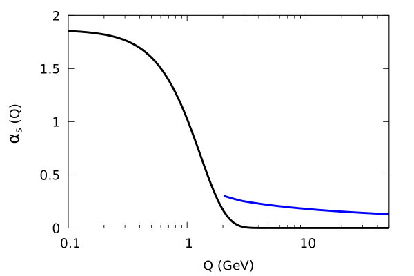
Figure 1: The black line represents an example of phenomenological nonperturbative strong coupling constant, that is $\alpha_{S}^{np}(Q)$ of Eq. (32) with the numerical vaues of the parameters given in Eq. (21); the blue line represents $\alpha_{S}^{p}(Q)$ of Eq. (28) that describes the experimental data in the perturbative region with the values of the parameters given in Eq. (31). The transition between the nonperturbative and perturbative regime is around $Q\simeq 2.0$ GeV.

5 Model I. Piecewise function

In this section, as a starting point of our exploration, we introduce a very simple definition of a (unique) strong coupling constant as a function of the momentum transfer $Q$. In this Model I, we consider a piecewise function of $Q$ with two intervals. We make the hypothesis that in the first interval, defined by $0\leq Q<\bar{Q}$, $\alpha_{S}(Q)$ is mostly related to the nonpertubative effects of the quark interaction. On the other hand, we assume that in the second interval, defined    by $Q\geq\bar{Q}$, $\alpha_{S}(Q)$ is given by the perturbative form of the QCD interaction. We require the continuity of $\alpha_{S}(Q)$ in $\bar{Q}$ and also the continuity of its first derivative, in the same point. The definition of the piecewise $\alpha_{S}(Q)$ function of the Model I is given by the following equation:

$$\alpha_{S}(Q)=\begin{cases}\alpha_{V}-\alpha_{G}+\alpha_{G}\exp\left(-{\frac{Q^{2}}{\tau^{2}}}\right)\text{for}~{}~{}0\leq Q<\bar{Q},\\ \alpha_{S}^{p}(Q)~{}\text{for}~{}~{}Q\geq\bar{Q}~{}.\end{cases}$$ (33)

As discussed above, the definition of the coupling constant function in the second interval is given exactly by the standard $\alpha_{S}^{p}(Q)$ of Eq. (28). Moreover, the parameters $b$ and $\Lambda$ are fixed and have the same numerical values of Eq. (31). In the first interval, as suggested by our previous studies [3, 5], we have a Gaussian term, proportional to $\alpha_{G}$; furthermore we have to add the constant contribution $\alpha_{V}-\alpha_{G}$. Note that, in this way, we have $\alpha_{S}(0)=\alpha_{V}$. The form of Eq. (33) has been chosen in order to reproduce the experimental data of the running coupling constant and to fit the charmonium spectrum.

The conditions of continuity of the function and of the first derivative, both calculated in $\bar{Q}$, give, respectively, the following equations:

$$\alpha_{V}-\alpha_{G}+\alpha_{G}\exp\left(-{\frac{{\bar{Q}}^{2}}{\tau^{2}}}\right)=\alpha_{S}^{p}({\bar{Q}})$$ (34)

$$-2\alpha_{G}{\frac{\bar{Q}}{\tau^{2}}}\exp\left(-{\frac{{\bar{Q}}^{2}}{\tau^{2}}}\right)=\alpha_{S}^{\prime p}({\bar{Q}})$$ (35)

where

$$\alpha_{S}^{\prime p}({\bar{Q}})=-~{}{\frac{2}{b{\bar{Q}}\ln^{2}\left({\frac{{\bar{Q}}^{2}}{\Lambda^{2}}}\right)}}$$ (36)

represents the first derivative of $\alpha_{S}^{p}(Q)$ calculated at $Q=\bar{Q}$.

In order to obtain the finite quark self-energy $\bar{V}_{V}$, we take the definition of Eq. (25) but perform the integral only up to $\bar{Q}$, disregarding the infinite contribution that would be obtained integrating from $\bar{Q}$ to $\infty$. It means that, for this Model I we have

$$\bar{V}_{V}={\frac{8}{3\pi}}\int_{0}^{\bar{Q}}dQ~{}\alpha_{S}(Q)~{}.$$ (37)

By means of the definition given in Eq. (33), this integral can be calculated analytically, obtaining the following expression:

$$\bar{V}_{V}={\frac{8}{3\pi}}\left[(\alpha_{V}-\alpha_{G})\bar{Q}+\alpha_{G}{\frac{\sqrt{\pi}}{2}}\tau\cdot\text{erf}\left({\frac{\bar{Q}}{\tau}}\right)\right]~{}.$$ (38)

We note that in Model I we have four parameters: $\alpha_{V},~{}\alpha_{G},~{}\tau$ and $\bar{Q}$ that are vinculated by the two conditions of Eqs. (34) and (35).
In Fig. 2 we plot $\alpha_{S}(Q)$ of the Model I. The charmonium spectrum is reproduced by using the scalar interaction and the mass interaction. The numerical values of the parameters, determined by the fit procedure, are shown respectively for the two interactions in the Column I S and I M of Tab. 1. We note that $\alpha_{V}$ is slightly bigger for case of the scalar interaction. The values of the constant $\tau$ of the Gaussian function are very similar in the two cases. Also the values of $\bar{Q}$ (that separates the perturbative and nonperturbative interval) are very similar for the scalar and the mass interaction. The quality of the fit of the spectrum, given by the parameter $\Theta$, that will be defined in Eq. (68), are displayed at the bottom of Tab. 1, showing that a better reproduction is obtained with the scalar interaction.

In summary, by means of Model I we have learned that a two interval piecewise function (constructed requiring continuity and first derivative continuity) can represent $\alpha_{S}(Q)$ for all the values of the momentum transfer $Q$. The value $\bar{Q}\simeq 2.362~{}GeV$ that separates the two intervals, is also used as integration limit to calculate the finite value of $\bar{V}_{V}$. In the first interval it was necessary to use a Gaussian function plus a constant term.

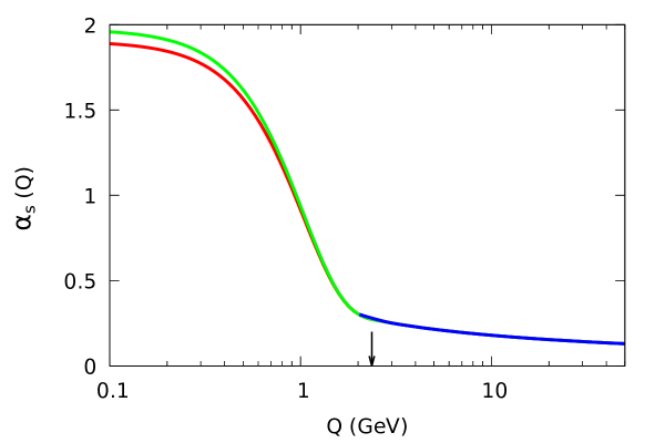
Figure 2: We plot $\alpha_{S}(Q)$ of Model I, defined in Eq. (33) with the conditions of Eqs. (34) and (35). To fit the charmonium spectrum we have used the scalar interaction with the parameters of the column (I S) of Tab. 1; in this case $\alpha_{S}(Q)$ is plotted with a red line. For the case of the mass interaction, with the parameters of the column (II S) of Tab. 1, $\alpha_{S}(Q)$ is plotted with a green line. The blue line represents the perturbative function $\alpha_{S}(Q)$ of Eq. (28), with the values of Eq. (31), that fits the experimental data. The arrow indicates the values of $\bar{Q}$ for the scalar and mass interaction. As given in Tab. 1 and discussed in Sect. 5, these two values are very close and are not distinguishable in this graphic.

6 Model II. One analytic function with the same definition for all the values of $Q$

In this model we try to represent the strong coupling constant as an analytic function with the same definition along the whole $Q$ axis. The simplest way to construct this function is to use the sum of a Gaussian function for the nonperturbative region “plus” a function that describes the perturbative behaviour of $\alpha_{S}(Q)$ at high $Q$. However, for the latter function it is not possible to take directly $\alpha_{S}^{p}(Q)$ of Eq. (28) because this function presents a singularity at $Q=\Lambda$. To “cure” this singularity we add the constant term $c_{L}>1$ to $Q^{2}/\Lambda^{2}$ in the argument of the logarithm. We denote this new function as $\xi_{L}(Q)$. In this way, we define $\alpha_{S}(Q)$ for the Model II, in the following form:

$$\alpha_{S}(Q)=(\alpha_{V}-\alpha_{L})\exp\left(-{\frac{Q^{2}}{\tau^{2}}}\right)+\xi_{L}(Q)$$ (39)

with

$$\xi_{L}(Q)={\frac{1}{b\ln\left(c_{{}_{L}}+{\frac{Q^{2}}{\Lambda^{2}}}\right)}}~{}.$$ (40)

Furthermore, we define $c_{L}$ as:

$$c_{{}_{L}}=\exp\left({\frac{1}{b~{}\alpha_{L}}}\right)~{}.$$ (41)

Note that, by means of the previous definition, $c_{{}_{L}}$ does not represent a new free parameter; furthermore its form has been chosen in such way that, in Eq. (40), $\xi_{L}(0)=\alpha_{L}$; in consequence, for the strong coupling constant of Model II, given by Eq. (39), we have $\alpha_{S}(0)=\alpha_{V}$. Finally, the numerical value of $b$ given in Eq. (31) and the value of $\alpha_{L}$ that will be obtained in the following, numerically give $c_{{}_{L}}>1$ so that, as discussed above, the function $\xi_{L}(Q)$ does not present any singularity. We conclude this discussion recalling that the parametrization of $\alpha_{S}(Q)$ given in Eq. (39) is similar to that adopted in Ref. [6].

To calculate the self-energy of the vector interaction $\bar{V}_{V}$ in Model II, we propose two different techniques, denoted as Technique A and Technique B. For the Technique A, we note that at high $Q$ (where the contribution of the Gaussian term is negligible), $\alpha_{S}(Q)$ of Eq. (39), due to the presence of $c_{L}$, is slightly less than $\alpha_{S}^{p}(Q)$ of Eq. (28); on the contrary, decreasing $Q$, $\alpha_{S}(Q)$ becomes greather than $\alpha_{S}^{p}(Q)$.
We can define, for the Technique A, $\bar{Q}$ as the value of momentum transfer for which the following equality is satisfied:

$$\alpha_{S}(\bar{Q})=\alpha_{S}^{p}(\bar{Q})~{}.$$ (42)

By using the expressions given in Eq. (39) and in Eq. (28), the value of $\bar{Q}$ can be determined numerically.

Then, for the calculation of the self-energy we can use the same expression used for Model I, that is Eq. (37), but integrating $\alpha_{S}(Q)$ of Eq. (39) up to the value $\bar{Q}$ determined by Eq. (42). In this way the finite self-energy is given by the nonperturbative effects that dominate at $Q\leq\bar{Q}$ while the infinite contribution given by the integration from $\bar{Q}$ to infinity is discarded.
The numerical results of the parameters that reproduce the experimental data of the strong coupling constant and fit the charmonium spectrum are shown in column (II A S) and (II A M) of Tab. 1 for the scalar and mass interaction, respectively. The behaviour of $\alpha_{S}(Q)$ is displayed in Fig. 3 where the procedure discussed above for finding $\bar{Q}$ is also illustrated.

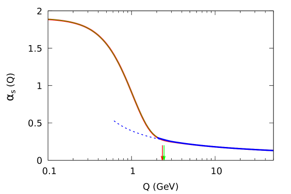
Figure 3: We plot $\alpha_{S}(Q)$ of Model II A (see Eqs. (39) -(41)) with the parameters of the scalar and mass interaction; a red and a green line are used for the two interactions, respectively. The two lines are partly superimposed. See Tab. 1, columns (II A S) and (II A M) for the values of the parameters in the two cases. The blue line represents $\alpha_{S}^{p}(Q)$. The dotted blue line represents this last function at low $Q$ and is plotted to illustrate the method used to find $\bar{Q}$. The values of this last quantity are represented by a red arrow and by a green arrow for the scalar and mass interaction, respectively.

In order to introduce the Technique B, we consider, in the first place, that the Gaussian function (that is the first term of $\alpha_{S}(Q)$ in Eq. (39) ) can be integrated up to infinity and gives a standard, finite contribution to the self-energy. This contribution can be calculated as in Eq. (26) but replacing $\alpha_{V}$ with $\alpha_{V}-\alpha_{G}$. However, also the second term of Eq. (39), that is $\xi_{L}(Q)$, “contains” some nonperturbative effects that give a contribution to the total self-energy. To calculate this contribution, we “approximate” (at low $Q$) the function $\xi_{L}(Q)$ with a Gaussian function of the form

$$\xi_{L}^{a}(Q)=\alpha_{L}\exp\left(-{\frac{Q^{2}}{\tau_{L}^{2}}}\right)$$ (43)

where the parameter $\tau_{L}$ is fixed in such way that the functions $\xi_{L}^{a}(Q)$ and $\xi_{L}(Q)$ have the same Taylor expansion up to order $Q^{2}$. The result for $\tau_{L}$ is the following:

$$\tau_{L}=\Lambda\left[{\frac{1}{b~{}\alpha_{L}}}\exp\left({\frac{1}{b~{}\alpha_{L}}}\right)\right]^{1/2}~{}.$$ (44)

By using Eq. (43) we calculate the corresponding self-energy in the standard way, integrating up to infinity. The total result for the self-energy calculated with the Technique B has the following analytic form:

$$\bar{V}_{V}={\frac{4}{3}}{\frac{1}{\sqrt{\pi}}}\left[\left(\alpha_{V}-\alpha_{L}\right)\tau+\alpha_{L}\tau_{L}\right]~{}.$$ (45)

The values of the parameters that reproduce $\alpha_{S}(Q)$ and fit the charmonium spectrum are given in the columns (II B S) amd (II B M) of Tab. 1, for the scalar and mass interaction, respectively. Note that the values of $\bar{V}_{V}$ obtained with Technique A and Technique B are very similar. The behaviour of the obtained $\alpha_{S}(Q)$ is shown in Fig. 4. We have checked that $\alpha_{S}(Q)$ of this Model II correctly gives the numerical values of Eqs. (27) and (30).

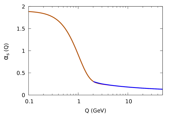
Figure 4: We plot $\alpha_{S}(Q)$ of Model II B for the scalar and mass interaction. The definitions and conventions are the same as in Fig. 3.

Summarizing the results of this section, we have learned that a unique function, with the same definition for all the values of $Q$, can reproduce the strong coupling constant of the quark-antiquark interaction. This function is represented by the sum of a Gaussian plus a regularized perturbative QCD function that gives a contribution also at low $Q$. We shall take into accont this last point for the study of Model III. The numerical results of Model II are similar to those of Model I corroborating the physical validity of the two models. The self-energy $\bar{V}_{V}$ for Model II can be calculated in two different ways: first, with the Technique A, by introducing (analogously to what learned in Model I), the quantity $\bar{Q}$ that, for this model, defines the upper limit of the integration; second, with the Technique B, we have also studied an analytic procedure that “extracts” the nonperturbative contribution from the second term of the function that represents $\alpha_{S}(Q)$. A procedure of the same kind well be used also in Model III. As shown in Tab. 1, columns (II A S), (II A M), (II B S) and (II B M), the numerical values of the parameters are similar, demonstrating that the two Techniques A and B are almost equivalent.

7 Model III. A differential equation for $\alpha_{S}(Q)$

In this section we obtain $\alpha_{S}(Q)$ as the solution of a (unique) differential equation that represents the low $Q$ and the high $Q$ physical behaviour of the strong coupling costant. This model is developed taking account of the results of the previous sections.

We start with some aspects related to notation and definitions.

• For clarity in the calculation of the derivatives, we prefer to use, in this section, the variable $t=Q^{2}$, in GeV².

• Only in the initial part of the model, we shall introduce the indices $l$ and $h$ for the low $t$ and high $t$ regions, respectively. For the strong coupling constant we have: $\alpha_{l}(t)$ and $\alpha_{h}(t)$. The reader can assume that, approximately, the low $t$ region is defined by $t\leq\bar{t}$ and the high $t$ region by $t>\bar{t}$, being $\bar{t}=\bar{Q}^{2}$, where $\bar{Q}$ has been introduced in the previous sections. In the final form of the model, we shall consider simultaneously all the values of $t$ and drop those indices.

• To simplify the intermediate mathematical calculations, we also introduce: $y_{S}(t)=1/\alpha_{S}(t)$, $y_{l}(t)=1/\alpha_{l}(t)$ and $y_{h}(t)=1/\alpha_{h}(t)$.

• Finally, we shall consider, in some expressions, $y_{S}$, $y_{l}$ and $y_{h}$ as independent variables and $t$ as a dependent variable.

We now study the differential equations for the strong coupling constant in the high $t$ and low $t$ regions, performing some transformations that allow to find a unique equation for the two cases.

We start from the low $t$ region, where, as suggested by the results of the previous sections, $\alpha_{l}(t)$ has essentially a Gaussian behaviour. It can be easily verified that $\alpha_{l}(t)$ satisfies the following differential equation

$${\frac{d\alpha_{l}(t)}{dt}}=-{\frac{1}{\tau^{2}}}\alpha_{l}(t)$$ (46)

The corresponding equation for $y_{l}(t)$ is:

$${\frac{dy_{l}(t)}{dt}}={\frac{1}{\tau^{2}}}y_{l}(t)$$ (47)

Taking $y_{l}$ as an independent wariable, we can write equivalently

$${\frac{dt}{dy_{l}}}=\tau^{2}{\frac{1}{y_{l}}}~{}.$$ (48)

For completeness we write the solution of the previous equation in the form:

$$t=\tau^{2}\ln(y_{l})+a_{l}$$ (49)

being $a_{l}$ the integration constant. With standard algebra one can verify that the Gaussian expression for $\alpha_{l}(t)$ is obtained:

$$\alpha_{l}(t)=\alpha_{l}(0)\exp\left(-{\frac{t}{\tau^{2}}}\right)$$ (50)

with

$$\alpha_{l}(0)=\exp(a_{l})~{}.$$ (51)

We now consider the high $t$ region where the strong coupling constant is given asymptotically by $\alpha_{S}^{p}(t)$ of Eq. (28). For this region, we have the following differential equation:

$${\frac{d\alpha_{h}(t)}{dt}}=-{\frac{b}{t}}\left[\alpha_{h}(t)\right]^{2}$$ (52)

where $b$ is the usual constant introduced in Sect. 4  with the numerical value given in Eq. (31) for our phenomenological calculation. At fundamental level, the previous differential equation represents the renormalization group equation for $\alpha_{S}(Q)$ at the leading order [19, 20, 21].

The corresponding equation for $y_{h}(t)$ is:

$${\frac{dy_{h}(t)}{dt}}={\frac{b}{t}}$$ (53)

Taking $y_{h}$ as an independent wariable, we can write equivalently

$${\frac{dt}{dy_{h}}}={\frac{t}{b}}$$ (54)

The solution has the form:

$$t=a_{h}\exp({\frac{y_{h}}{b}})$$ (55)

where $a_{h}$ is the integration constant. To reproduce the experimental data in the perturbative regime, we set

$$a_{h}=\Lambda^{2}$$ (56)

where $\Lambda$ is the usual QCD scale introduced in Sect. 4  with the numerical phenomenological value given in Eq. (31). With standard passages, one can verify that $\alpha_{h}(t)$ takes the form:

$$\alpha_{h}(t)=\alpha_{S}^{p}(t)$$ (57)

where $\alpha_{S}^{p}(t)$ is the perturbative expression of Eq. (28).

Taking into account the specific form of Eqs. (48) and (54), we can write a unique differential equation that holds for all the values of $t$, that is:

$${\frac{dt}{dy_{S}}}=\tau^{2}{\frac{1}{y_{S}}}+{\frac{t}{b}}+k~{}.$$ (58)

In the r.h.s. of the previous equation, the second term $t/b$ is dominant at high $t$, while the first term contributes essentially at low $t$. We have also introduced the additional constant term $k$, in GeV². This term will be related to the other parameters of Model III in Eq. (64); we shall also discuss in the following its physical relevance. Here we note that, in Eq. (58), this constant term $k$ is negligible at high $t$; on the other hand, it does not alter too much the low $t$ behaviour that is given by the first term of the previous equation. We have used the symbol $\tau$ in the first term of Eq. (58) even though we shall not obtain a Gaussian term in the solution. In this sense, $\tau$ has here a different meaning with respect to Model I and Model II.

In conclusion, Eq. (58) represents the “unique” differential equation for the strong coupling constant of our Model III. The same equation can be rewritten as a differential equation for $\alpha_{S}(t)$ in the following form:

$${\frac{d\alpha_{S}(t)}{dt}}=-\left[\alpha_{S}(t)\right]^{2}{\frac{1}{\tau^{2}\alpha_{S}(t)+{\frac{t}{b}}+k}}~{}.$$ (59)

We shall check that, with the solution for our model, the denominator in the r.h.s of the previous equation does not vanish and $\alpha_{S}(t)$ does not present any singularity.

The solution of Eq. (59) is easily found with the help of of Maxima - A Computer Algebra System, in the following implicit form:

$$t+kb=\left[a_{S}-\tau^{2}\Gamma\left(0,{\frac{1}{b\alpha_{S}(t)}}\right)\right]\exp\left({\frac{1}{b\alpha_{S}(t)}}\right)~{}$$ (60)

where it has been introduced the incomplete gamma function $\Gamma(0,x)$ whose properties can be found in Ref. [22]. In particular, we recall

$$\Gamma(0,x)=\int_{x}^{\infty}{\frac{\exp(-v)}{v}}dv$$ (61)

given by Eq. (8.350.1) of Ref. [22]. In consequence, one has for the derivative

$${\frac{d\Gamma(0,x)}{dx}}=-{\frac{\exp(-x)}{x}}~{}.$$ (62)

By means of this last equation, one can easily check that the expression of Eq. (60) really represents a solution of Eq. (58).

The integration constant $a_{S}$ of Eq. (60) is determined by comparing that equation, at large $t$, with Eq. (55) and using the same definition given in Eq. (56), that is:

$$a_{S}=\Lambda^{2}~{}.$$ (63)

In this way, the correct high $t$ behaviour of $\alpha_{S}(t)$ is obtained. In order to determine the constant parameter $k$, we calculate Eq. (60) at $t=0$. Using Eq. (63) and the definition $\alpha_{S}(0)=\alpha_{V}$, we obtain the following expression:

$$k=\left[\Lambda^{2}-\tau^{2}\Gamma\left(0,{\frac{1}{b\alpha_{V}}}\right)\right]\exp\left({\frac{1}{b\alpha_{V}}}\right)~{}.$$ (64)

We note that the parameter $k$ is related to $\alpha_{V}$. In this way, due to the presence of $k$, it is possible to fix $\alpha_{V}$ at the value $\alpha_{V}\simeq 2$ that is needed to reproduce the charmonium spectrum. In the following we shall see that $k$ takes a negative value. We observe that, at low $Q$, $\alpha_{S}(Q)$ is not given exactly by a Gaussian function of $Q$. In this respect, we recall that also in Model I we had a Gaussian plus a constant term and in Model II we had a Gaussian plus a regularized perturbative QCD function.

In summary, Eq. (60) represents the implicit solution of Eq. (59); the integration constant $a_{S}$ is given by Eq. (63) and the parameter $k$ is given by Eq. (64). The only two free parameters of this model are $\alpha_{V}$ and $\tau$.

For the following calculations, we have to invert numerically Eq. (60) to obtain $\alpha_{S}(t)$.

We now have to calculate the finite self-energy $\bar{V}_{V}$. To this aim, we take advantage of the Model II, Technique B. We “approximate”, at low $t$, $\alpha_{S}(t)$, with the following function:

$$\alpha_{S}^{a}(t)=\alpha_{V}\exp\left(-{\frac{t}{\tau_{S}^{2}}}\right).$$ (65)

We also require that $\alpha_{S}(t)$ (implicitly defined in Eq. (60) ) and $\alpha_{S}^{a}(t)$ have the same Taylor expansion up to orden $t=Q^{2}$. With standard calculations, one finds that this condition is satisfied when the parameter $\tau_{S}$ has the following form:

$$\tau_{S}=\left(\tau^{2}+{\frac{k}{\alpha_{V}}}\right)^{\frac{1}{2}}~{}.$$ (66)

Then, $\bar{V}_{V}$ is obtained, as in Eq. (25), integrating $\alpha_{S}^{a}(t)$ up to infinity. The result is:

$$\bar{V}_{V}={\frac{4}{3}}\alpha_{V}{\frac{\tau_{S}}{\sqrt{\pi}}}$$ (67)

The values of the parameters that reproduce $\alpha_{S}(Q)$ and fit the charmonium spectrum are given in the columns (III S) amd (III M) of Tab. 2, for the scalar and mass interaction, respectively. The behaviour of the obtained $\alpha_{S}(Q)$ is shown in Fig. 5. We have checked that $\alpha_{S}(Q)$ obtained by solving the differential equation of this model correctly gives the numerical values of Eqs. (27) and (30).

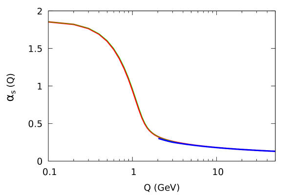
Figure 5: We plot $\alpha_{S}(Q)$ of Model III for the scalar and mass interaction. The definitions and conventions are the same as in Fig. 3.

8 The results of the charmonium spectrum

We give here some details about the reproduction of the charmonium spectrum and comment the results of the calculations. The technique for solving the RDLE of Sect. 2 and the procedure to fit the experimental data [19] are exactly the same as in our previous works [2, 3, 5, 6]. For the mass of the quark we have taken the value $m_{q}=1.273$ GeV. This value represents the charm quark mass renormalized at the $\overline{MS}$ mass [19].

The vector potential function $V_{V}(r)$ is calculated performing numerically the Fourier transform of Eq. (15) for each model of $\alpha_{S}(Q)$. The results obtained for the different models are very similar, so that we only show in Figs. 6 and 7 the results for the Model II B M and III S, respectively. For comparison, we also plot, in the same figures, the pure Coulombic potential functions observing that, at large $r$, our potential functions go to zero exactly as the Coulombic ones. Also the quark vector self-energy $\bar{V}_{V}$ is calculated according to the specifications of each model.

Figure 6: The blue line represents the vector potential function $V_{V}(r)$ for the model II B M; the black line represents the Coulombic potential with the same $\alpha_{V}$ of the Model II B M. The two functions coincide for large $r$.

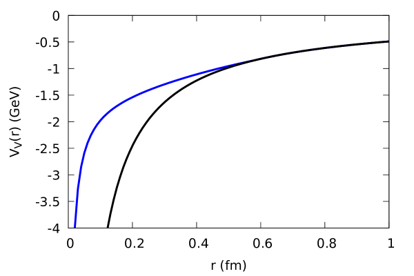
Figure 7: The vector function potential $V_{V}(r)$ for the Model III S; the conventions are the same as in Fig. 6.

The $X$-potential function $V_{X}(r)$ has the (negative) Gaussian form given in Eq. (10). The parameter $\bar{V}_{X}$ is determined, in this work, by means of Eq. (11). On the other hand, in Ref. [5], the value of $\bar{V}_{X}$ was fixed at $0.735$ GeV, phenomenologically related to the excitation of the first two scalar meson resonances that have the vacuum quantum numbers [19]: the $f_{0}(500)$ with the mass peak at (roughly) $M[f_{0}(500)]=0.475$ GeV and the $f_{0}(980)$ with the mass peak at (roughly) $M[f_{0}(980)]=0.995$ GeV. Being (indicatively) the mean value of these two mass peaks at $<M_{0}>=0.735$ GeV, we took, in that work [5], $\bar{V}_{X}=<M_{0}>$. In this work, $\bar{V}_{X}$ is determined by Eq. (11); as shown in Tabs. 1 and 2, it assumes values not far from $<M_{0}>$ and, in any case, it belongs to the interval given by the first two scalar resonaces, that is: $M[f_{0}(500)]<\bar{V}_{X}<M[f_{0}(980)]$.

For the quality of the fit, as in [5, 6], we have defined

$$\Theta=\sqrt{{\frac{\sum_{k}(E_{k}^{th}-M_{k}^{exp})^{2}}{N_{d}}}}~{},$$ (68)

where $E_{k}^{th}$ and $M_{k}^{exp}$ respectively represent the result of the theoretical calculation and the experimental value of the mass, for the $k$-th resonance and $N_{d}=16$ is the number of the fitted resonances.

The spectra obtained with the different models are very similar. For this reason we only give in Tab. 3 the results of Model II B M and III S.

For completeness, we also note that, as in [5], it is not possible to reproduce the resonance $\chi_{c0}(3915)$. The new experimental data [19] give, for this resonance, a mass of $3922.1\pm 1.8$ MeV. Our model, taking the quantum numbers $2^{3}P_{0}$, gives the mass values of $3846$ MeV and $3857$ MeV, for the models II B M and III S, respectively. Our model and other quark models give a wrong order for the masses of this resonance and its partner $\chi_{c1}(3872)$. A possible solution of this problem has ben proposed by using three-body forces in the framework of a phenomenological nonrelativistic model [17].

Concerning the general structure of our interaction, we note that (neglecting the spin dependent terms and recalling that $V_{V}(r)$ goes to zero as the Coulombic potential) the maximum value of the total vector potential $\bar{V}_{V}+V_{V}(r)$ is given by $\bar{V}_{V}$. In consequence, the maximum value for the mass of a bound state is, roughly, $M_{max}=\bar{V}_{V}+2m_{q}$. As shown in Tab. 1, $\bar{V}_{V}$ assumes slightly different values in the different models. Taking, indicatively, $\bar{V}_{V}=1.83$ GeV, we have the numerical value $M_{max}\approx 4.376$ GeV. Comparing this result with the analysis of the experimental data given in Ref. [19], we note that the only state with the properties of a conventional $c\bar{c}$ state and with a value of mass greater than $M_{max}$, would be the $\psi(4415)$. This fact indicates that our value of $M_{max}$ (that represents the highest value of mass for which our $c\bar{c}$ model can be safely applied) is approximately in accordance with the experimental findings. At higher values of mass, new physical effects should be taken into account [15, 16, 17, 18] and an explicit mechanism for confinement should be introduced.

We conclude this paper with the following considerations. The momentum dependence of $\alpha_{S}(Q)$ given by perturbative QCD, in accordance with high $Q$ experimental data, can be matched with the phenomenological behaviour of the same quantity at low $Q$. By discarding an infinite contribution, the vector quark finite self-energy can be consistently calculated. In this way the charmonium spectrum is accurately reproduced. Further investigation is necessary to establish a deeper connection between the effective bound state quark interaction and the phenomenology related to the QCD analysis.

Table 1: Numerical values of the parameters of Model I and Model II; for more details and for the definitions of the parameters $\alpha_{V},~{}\tau,~{}\alpha_{G},~{}\alpha_{L},~{}\bar{Q}$ and $\tau_{L}$ see Sect. 5 and Sect. 6. The quark mass $m_{q}$ is fixed at the value of Ref. [19]. $\bar{V}_{V}$ is the vector quark self-energy. For the scalar or mass interaction of Eq. (10), the parameter $\bar{V}_{X}$ is determined by Eq. (11), $r_{X}$ is a fit parameter. The parameter $\Theta$, defined in Eq. (68), gives the quality of the fit.

							Units
$m_{q}$	$1.273$						GeV
$\Lambda$	$0.1462$						GeV
$b$	$0.65842$
Model	I S	I M	II A S	II A M	II B S	II B M
$\alpha_{V}$	$1.9036$	$1.9740$	$1.9010$	$1.9042$	$1.8997$	$1.8994$
$\tau$	$1.0405$	$1.0361$	$1.0199$	$1.0238$	$1.0196$	$1.0204$	GeV
$\alpha_{G}$	$1.6401$	$1.7105$
$\alpha_{L}$			$0.39802$	$0.44694$	$0.37300$	$0.36462$
$\bar{Q}$	$2.3608$	$2.3629$	$2.3379$	$2.4496$			GeV
$\tau_{L}$					$2.2599$	$2.3951$	GeV
$\bar{V}_{V}$	$1.8100$	$1.8600$	$1.8045$	$1.8340$	$1.80505$	$1.8350$	GeV
$\bar{V}_{X}$	$0.73000$	$0.68000$	$0.73546$	$0.70596$	$0.73495$	$0.70496$	GeV
$r_{X}$	$1.8437$	$2.0041$	$1.8022$	$1.8718$	$1.8097$	$1.8894$	fm
$\Theta$	$12.5$	$14.0$	$12.9$	$12.2$	$12.9$	$12.0$	MeV

Table 2: Numerical values of the parameters of Model III. The values of the quark mass $m_{q}$, $\Lambda$ and $b$, not shown here, are exactly the same as in Tab. 1. For more details, in particular for the definitions of $\tau,~{}k$ and $\tau_{S}$, see Sect. 7. For the meaning of the other parameters also see Tab. 1.

			Units
Model	III S	III M
$\alpha_{V}$	$1.8647$	$1.8659$
$\tau$	$1.9146$	$1.9501$	GeV
$k$	$-3.7306$	$-3.8781$	GeV2
$\tau_{S}$	$1.2904$	$1.3145$	GeV
$\bar{V}_{V}$	$1.8100$	$1.8450$	GeV
$\bar{V}_{X}$	$0.729955$	$0.69503$	GeV
$r_{X}$	$1.8732$	$1.9852$	fm
$\Theta$	$12.55$	$14.01$	MeV

Table 3: Comparison between the theoretical results of the charmonium spectrum and the experimental average values [19], listed in the last column. As examples, we only show (in the corresponding columns) the results of the models II M B and III S, respectively studied in Sects. 6 and 7. The values of the parameters used for these models can be found in Tabs. 1 and 2. The quantum numbers $n$, $L$, $S$ and $J$, introduced in Ref. [3], respectively represent the principal quantum number, the orbital angular momentum, the spin and the total angular momentum. A line divides the resonances below and above the open Charm threshold.

Name	$n^{2S+1}L_{J}$	II M B	III S	Experiment
$\eta_{c}(1S)$	$1^{1}S_{0}$	2983	2984	2984.1 $\pm$ 0.4
$J/\psi(1S)$	$1^{3}S_{1}$	3113	3099	3096.9 $\pm$ 0.006
$\chi_{c0}(1P)$	$1^{3}P_{0}$	3403	3420	3414.71 $\pm$ 0.30
$\chi_{c1}(1P)$	$1^{3}P_{1}$	3497	3503	3510.67 $\pm$ 0.05
$h_{c}(1P)$	$1^{1}P_{1}$	3514	3516	3525.37 $\pm$ 0.14
$\chi_{c2}(1P)$	$1^{3}P_{2}$	3572	3565	3556.17 $\pm$ 0.07
$\eta_{c}(2S)$	$2^{1}S_{0}$	3630	3638	3637.7 $\pm$ 0.9
$\psi(2S)$	$2^{3}S_{1}$	3681	3679	3686.097 $\pm$0.011
$\psi(3770)$	$1^{3}D_{1}$	3790	3797	3773.7 $\pm$ 0.7
$\psi_{2}(3823)$	$1^{3}D_{2}$	3827	3829	3823.51 $\pm$ 0.34
$\chi_{c1}(3872)$	$2^{3}P_{1}$	3890	3895	3871.64 $\pm$ 0.06
$\chi_{c2}(3930)$	$2^{3}P_{2}$	3933	3929	3922.5 $\pm$ 1.0
$\psi(4040)$	$3^{3}S_{1}$	4015	4013	4040 $\pm$ 4
$\chi{c1}(4140)$	$3^{3}P_{1}$	4147	4145	4146.5 $\pm$ 3.0
$\psi(4230)$	$4^{3}S_{1}$	4221	4211	4222.1 $\pm$ 2.3
$\chi{c1}(4274)$	$4^{3}P_{1}$	4287	4269	4286 $\pm$ 9

References

- [1] M. De Sanctis, Front. Phys. 7, 25 (2019).
- [2] M. De Sanctis, Acta Phys. Pol. B 52, 125 (2021).
- [3] M. De Sanctis, Acta Phys. Pol. B 52, 1289 (2021).
- [4] M. De Sanctis, Acta Phys. Pol. B 53, 7A-2 (2022).
- [5] M. De Sanctis, Acta Phys. Pol. B 54, 1A-2 (2023).
- [6] M. De Sanctis, Acta Phys. Pol. B 54, 10A-3 (2023).
- [7] A. Deur, V. Burkert, J.P. Chen and W. Korsch, “Experimental determination of the effective strong coupling constant”, Phys.Lett. B 650, 244 (2007); arXiv:hep-ph/0509113v3, (2007).
- [8] A. Deur, V. Burkert, J.P. Chen and W. Korsch, “Determination of the effective strong coupling constant from CLAS spin structure function data”, Phys.Lett.B 665, 349 (2008); arXiv:hep-ph/0803.4119v2, (2008).
- [9] A. Deur, V. Burkert, J.P. Chen and W. Korsch, “Experimental determination of the QCD effective charge ”, Particles 5(2), 171 (2022); arXiv:2205.01169v2 [hep-ph] (2022).
- [10] A. Deur, S. J. Brodsky and G. F. de Téramond, “ The QCD running coupling”, Progress in Particle and Nuclear Physics, 90, 1 (2016).
- [11] A. Deur, S. J. Brodsky and C. D. Roberts, “QCD Running Couplings and Effective Charges” arXiv:2303.00723v1 [hep-ph] (2023), Review commissioned by Progress in Particle and Nuclear Physics.
- [12] Shwe Sin Oo, Sungwook Lee and Khin Maung Maung, “Modified Coulomb potential and the S-state wavefunction of heavy quarkonia” arXiv:2406.06790v1 [hep-ph] (2024).
- [13] H. Cancio and P. Masjuan, “The Holographic QCD Running Coupling Constant from the Ricci Flow” arXiv:2408.00455 [hep-ph] (2024).
- [14] J. L. Richardson, Phys. Lett. B 82, 272 (1979).
- [15] Chaitanya Anil Bokade and Bhaghyesh, “Charmonium: Conventional and XYZ States in a Relativistic Screened Potential Model”, arXiv:2408.06759v1 [hep-ph] (2024).
- [16] J. Ferretti and E. Santopinto. “Quark structure of the X(4500), X(4700) and states”, arXiv:2104.00918v1 [hep-ph] (2021).
- [17] Sungsik Noh, Aaron Park, Hyeongock Yun, Sungtae Cho and Su Houng Lee, “The Inevitable Quark Three-Body Force and its Implications for Exotic States”, arXiv:2408.00715v1 [hep-ph] (2024).
- [18] M. Berwein, N. Brambilla, A. Mohapatra and A. Vairo “One Born-Oppenheimer Effective Theory to rule them all: hybrids, tetraquarks, pentaquarks, doubly heavy baryons and quarkonium”, arXiv:2408.04719v1 [hep-ph] (2024).
- [19] S. Navas et al. (Particle Data Group), Phys. Rev. D 110, 030001 (2024)
- [20] G. M. Prosperi, M. Raciti and C. Simolo, Prog. Part. Nucl. Phys. 58 387 (2007), arXiv:hep-ph/0607209.
- [21] J. Campbell, J. Huston, F. Krauss, The Black Book of Quantum Chromodynamics, A Primer for the LHC Era, Oxford University Press, Oxford U.K.(2018).
- [22] I.S. Gradshteyn and I.M. Ryzhik, “Table of integrals, series and products”, Academic Press, New York, (1980).