Spin-1 Haldane phase in a chain of Rydberg atoms

Abstract

We present a protocol to implement a spin-1 chain in Rydberg systems using three Rydberg states close to a Förster resonance. In addition to dipole-dipole interactions, strong van der Waals interactions naturally appear due to the presence of the Förster resonance and give rise to a highly tunable Hamiltonian. The resulting phase diagram is studied using the infinite density-matrix renormalization group and reveals a highly robust Haldane phase – a prime example of a symmetry protected topological phase. We find experimentally accessible parameters to probe the Haldane phase in current Rydberg systems, and demonstrate an efficient adiabatic preparation scheme. This paves the way to probe the remarkable properties of spin fractionalization in the Haldane phase.

I Introduction

Topological phases in quantum many-body systems exhibit intriguing properties like anyonic excitations, topological order, string order, edge states and fractionalization [1]. Many of these topological phases that are currently studied theoretically as well as experimentally, like the fractional quantum Hall state [2] and spin liquids [3, 4], occur in two or higher dimensional systems. For one-dimensional systems, it was shown that such topologically ordered phases do not exist [5]. However, so-called symmetry protected topological (SPT) phases can appear in one dimension and still feature many similar properties. Thus, such one-dimensional SPT phases can often be used to get a better understanding of these topological properties. A prime example for this is the spin-1 Haldane phase [6, 7] and its characteristic AKLT state [8], which introduced the concept of Valence Bond Solids (VBS) and hidden order. Its most intriguing property, however, is the appearance of fractionalized spins at the edges. In this letter, we propose a scheme to realize such a spin-1 Haldane phase using Rydberg atoms and provide insights into how to detect the fractional spin states in an experiment.

In recent decades, there has been significant progress in studying quantum many-body systems using artificial matter platforms [9] such as cold atoms [10], ion traps [11], and Rydberg atoms [12]. Rydberg atoms, in particular, offer a promising platform for exploring strongly correlated quantum many-body systems due to their highly tunable interactions, including dipole-dipole and van der Waals interactions [13, 14, 15, 16, 17, 18, 4]. Additionally, the use of optical tweezers allows for precise control over individual atoms [19, 20, 21, 22]. Various quantum many-body phases have already been realized in such Rydberg systems in recent years, ranging from the one-dimensional SSH chain [14] to two-dimensional quantum Ising models [23], and even signatures of spin liquids have been observed in Rydberg systems [4]. While most implemented models reduce each Rydberg atom to an effective two-level system, there also are theoretical proposals that utilize three levels in a V-shaped configuration to implement two hard-core bosonic particles [24]. In the presence of Förster resonances [25, 26], equidistant three-level systems are realized, leading to additional dipole-dipole interactions and van der Waals terms [27, 28, 29].

Here, we present a detailed study on how these three Rydberg states, when close to a Förster resonance, can be used to implement an effective spin-1 system. The typical dipole-dipole and van der Waals interactions of these Rydberg states can then be mapped to spin-1 operators, resulting in an effective spin-1 Hamiltonian. By tuning the various parameters of the Rydberg system we can access different regimes in the phase diagram of the spin-1 model. We study the different phases using the infinite density-matrix renormalization group (infinite DMRG) and demonstrate the appearance of the Haldane phase for experimentally realistic parameters. Furthermore, we show that the ground state of the Haldane phase can be adiabatically prepared by starting from a product state and applying a staggered, effective magnetic field. Signatures of the Haldane phase, such as the string order parameter and edge states, can be experimentally observed through site-resolved measurements of the local spins. While some experimental signatures of the Haldane phase have already been observed in the topological equivalent SSH chain using qubit systems [14, 30], the Förster resonance enables us to implement a spin-1 chain and thus allow us to additionally study the fractionalization of the edge spin degrees of freedoms in the Haldane phase.

II System and Model

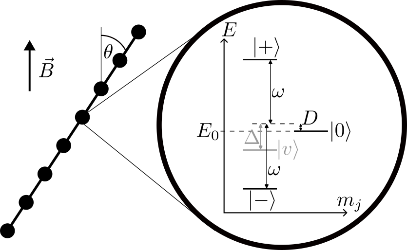
Figure 1: Sketch of the one-dimensional chain of Rydberg atoms aligned at an angle $\theta$ with respect to the magnetic field $\vec{B}$. In addition, a simplified level structure of the Rydberg atoms is shown. This includes the three main states $\ket{+},\ket{0},\ket{-}$, which are defined in eq. 2. Furthermore, an additional nearby state $\ket{v}$ is shown, which explains the dominant part of the van der Waals interactions.

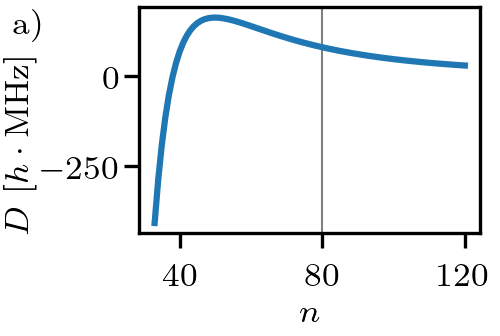
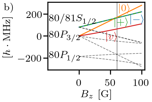
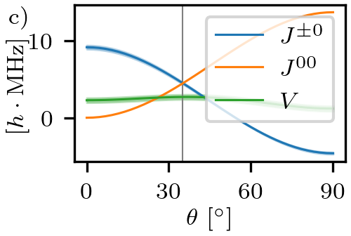
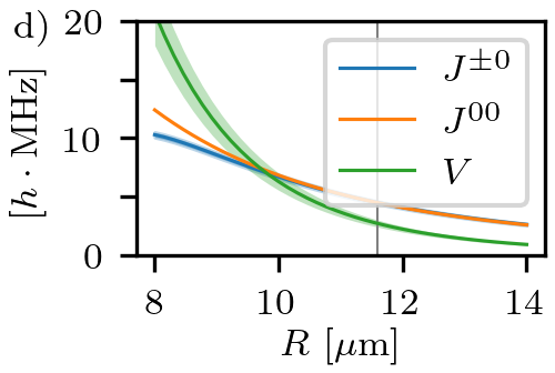
Figure 2: a) The anisotropy energy $D$ (without any fields applied) for the states defined in eq. 2. b) The energy spectrum of the Rydberg Zeeman sublevels of interest in a rotating frame with respect to the energy $E_{0}$ of the state $\ket{0}$ at $B=0$ (i.e. the $80S_{1/2}$ and $81S_{1/2}$ manifolds are shifted by $\pm\omega$ and thus lie on top of each other). c) and d) The interaction strengths $J^{\pm 0}$, $J^{00}$ and $V$ over c) the angle $\theta$ between the magnetic field and the interatomic axis and d) the interatomic distance $R$. For c) and d) we applied a magnetic field of $B=60.7\,\mathrm{G}$ and the distance (angle) was fixed at $R=11.6\,\mathrm{\mu m}$ ($\theta=35.1\,\mathrm{{}^{\circ}}$). The blue shaded area around the $J^{\pm 0}$ line indicates the difference of the $J^{+0}$ and $J^{-0}$ interaction strengths and the green shaded area around the $V$ line indicates the difference of the $V^{\text{diag}}$ and $V^{\text{offd}}$ interaction strengths. The gray vertical lines in the individual plots indicate the values used in section IV. All results in this figure are calculated via the pairinteraction software [31].

Our system, which is sketched in fig. 1, consists of a one-dimensional chain of Rydberg atoms. Each atom can effectively be described by three states $\ket{+},\ket{0},\ket{-}$ and thus describes a spin-1 degree of freedom. Note that we label our Rydberg states already like spin-1 states, but in principle for each state we have a set of quantum numbers $\ket{n,l,j,m_{j}}$ that describe the Rydberg state, which are quantized along the magnetic field $\vec{B}=B\vec{e_{z}}$. To isolate the three Rydberg states, as well as to tune the energies and interactions, we tune the strength of the magnetic field $B$, and change the angle $\theta$ of the interatomic axis with respect to the magnetic field.

In the following we show that the many-body Hamiltonian of this Rydberg system for a proper choice of the parameters can effectively be described by a spin-1 Hamiltonian, which is given by

$$H =\frac{1}{2}\sum_{i\neq j}\frac{J^{xy}}{r_{ij}^{3}}\left(S^{x}_{i}S^{x}_{j}+S^{y}_{i}S^{y}_{j}\right)+D\sum_{i}(S^{z}_{i})^{2}$$

$$\quad+\frac{1}{4}\sum_{i\neq j}\frac{V}{r_{ij}^{6}}\Bigl{[}(S^{+}_{i})^{2}(S^{-}_{j})^{2}+(S^{z}_{i}S^{z}_{j}-1)S^{z}_{i}S^{z}_{j}\Bigr{]}\,.$$ (1)

The $S^{x,y,z,\pm}$ are spin-1 operators and are explicitly defined in appendix A. $J^{xy}$ is the dipole-dipole interaction strength, $D$ is the anisotropy energy, and $V$ is the van der Waals interaction strength. Note that throughout this paper, we express all energies as frequencies in units of $h\cdot\mathrm{MHz}$, where $h$ is the Planck constant.

While the Haldane phase was originally introduced for the $SO(3)$ symmetric Heisenberg model [6, 7], it was later shown that even the dihedral symmetry $D_{2}$ ($=\mathbb{Z}_{2}\times\mathbb{Z}_{2}$) or time reversal symmetry can protect the Haldane phase [5, 32]. The $D_{2}$ symmetry is a subgroup of the $SO(3)$ symmetry and consists of all $\pi$ rotations around the $x$-, $y$- and $z$-axis. The Hamiltonian (1) respects this dihedral symmetry $D_{2}$ as well as time reversal symmetry. It was shown that the spin-1 XXZ-D model [this corresponds to the first line of eq. 1 and an additional coupling $J^{z}S^{z}_{i}S^{z}_{j}$] for only nearest neighbor interactions does only feature the Haldane phase for $J^{z}>0$ [33]. By adding long range interactions one can stabilize the Haldane phase for the antiferromagnetic spin-1 XXZ model [34] also for $J^{z}=0$. However, the signatures in the region $J^{z}=0$ are rather weak, and it is not clear, whether the Haldane phase could be measured in a finite size experiment. Here, we demonstrate that natural strong van der Waals terms appear due to the Förster resonance. These additional terms can further stabilize the Haldane phase and make it more accessible in a real experiment. We emphasize that the van der Waals term consists of multiple parts: One term, which is proportional to $S^{z}_{i}S^{z}_{j}$, and thus drives the model closer to the Heisenberg point, possibly resulting in a more stable Haldane phase; and a second term, which is proportional to $(S^{+}_{i})^{2}(S^{-}_{j})^{2}+(S^{-}_{i})^{2}(S^{+}_{j})^{2}$. This second term is also part of the famous AKLT Hamiltonian [8], and thus can stabilize the Haldane phase.

In the remainder of this section we motivate and explain the three terms $D$, $J^{xy}$ and $V$ in more detail on the level of the Rydberg states. A mapping of the Rydberg interactions of the three states $\ket{+},\ket{0},\ket{-}$ to spin-1 operators used in eq. 1 can be found in appendix A.

Anisotropy energy

Ignoring a global energy shift $E_{0}$, we have two energies in this system: $\omega=(E_{+}-E_{-})/2$ and $D=(E_{+}+E_{-})/2-E_{0}$ (see fig. 1). For the states we are interested in, the energy difference $\omega$ is much larger than the anisotropy energy $D$. This allows us to treat the system as a spin-1 system, where the $z$-component of the total magnetization $M_{\mathrm{tot}}=\left\langle\sum_{i}S^{z}_{i}\right\rangle$ is conserved.

To achieve this desired energy structure, we propose to use the following configuration of Rydberg states

$$\ket{+} =\ket{(n+1)S_{1/2},m_{j}=+1/2}\,,$$

$$\ket{0} =\ket{nP_{3/2},m_{j}=+3/2}\,,$$

$$\ket{-} =\ket{nS_{1/2},m_{j}=+1/2}\,.$$ (2)

In fig. 2 a), one can see that for different values of $n$ we are indeed close to so-called Förster resonances, where the anisotropy energy $D$ is small compared to the energy difference $\omega$, which for $n=80$ is $\omega/h\approx 7\,\mathrm{GHz}$. In the following we focus on the case $n=80$. However, the results are qualitatively the same for other choices of $n$. By applying a magnetic field $B$ we induce a Zeeman shift on all states, which splits the different magnetic sublevels and also tunes the anisotropy energy $D$. This can be seen in fig. 2 b), where we plotted the $80S_{1/2}$ and $81S_{1/2}$ in a rotating frame (shifted by the energy $\pm\omega$) together with the $80P_{3/2}$ and $80P_{1/2}$ manifolds. For magnetic fields $B\approx 60\,\mathrm{G}$ the three states $\ket{+}$, $\ket{0}$ and $\ket{-}$ are nearby degenerate and well separated from the other Zeeman sublevels, which are plotted as gray dashed lines.

The choice of the quantum numbers $l$, $j$ and $m_{j}$ above is partly motivated by the Förster resonance and partly motivated by constructing exactly the following Rydberg interactions that map to typical spin-1 interactions.

Dipole-dipole interactions

The allowed dipole-dipole interactions in our Rydberg system are
$\ket{+0}\xrightarrow{d_{i}^{+}d_{j}^{-}}\ket{0+}$ with strength

$$J^{+0}=\frac{3\cos^{2}\theta-1}{2r^{3}}\left|\bra{0}d^{+}\ket{+}\right|^{2}\,,$$

$\ket{-0}\xrightarrow{d_{i}^{+}d_{j}^{-}}\ket{0-}$ with strength

$$J^{-0}=\frac{3\cos^{2}\theta-1}{2r^{3}}\left|\bra{0}d^{+}\ket{-}\right|^{2}\,,$$

and $\ket{+-}\xrightarrow{d_{i}^{+}d_{j}^{+}}\ket{00}$ and $\ket{-+}\xrightarrow{d_{i}^{+}d_{j}^{+}}\ket{00}$ with strength

$$J^{00}=\frac{-3\sin^{2}\theta}{2r^{3}}\bra{0}d^{+}\ket{-}\bra{0}d^{+}\ket{+}$$

as well as all hermitian conjugates. Here, the $d^{\pm}$ are the dipole operators of the Rydberg states, acting on the total angular momentum $j$ and $m_{j}$.

For large principal quantum numbers $n$, the dipole moment of the $\ket{nS_{1/2}}$ and $\ket{(n+1)S_{1/2}}$ differ only by a small amount (more specifically $\bra{0}d^{+}\ket{+}\approx-\bra{0}d^{+}\ket{-}$), which results in $J^{+0}\approx J^{-0}$. Thus, we can define $J^{\pm 0}=(J^{+0}+J^{-0})/2$ and ignore for now the effect of a non-vanishing $\delta^{\pm 0}=(J^{+0}-J^{-0})/2$.

Furthermore, we find that $J^{00}$ can be easily tuned compared to $J^{\pm 0}$ by changing the angle $\theta$ of the applied magnetic field, as shown in fig. 2 c). While this in principle gives rise to an additional degree of freedom in our model, in this work we only focus on the case $J^{00}=J^{\pm 0}$. The angle for this can be estimated by setting $3\cos^{2}\theta-1=3\sin^{2}\theta$. Taking the full effective Rydberg pair Hamiltonian into account (see appendix C) we find $J^{00}=J^{\pm 0}$ to be fulfilled for $\theta\approx 35.1\,\mathrm{{}^{\circ}}$.

As detailed in appendix A the combined action of the three terms $J^{+0}=J^{-0}=J^{00}$ can be mapped to the spin-1 XY interaction $J^{xy}$ in eq. 1.

Van der Waals interactions

In real Rydberg systems we have more than three states, which also give rise to van der Waals interactions due to the coupling to additional Rydberg states. Often the van der Waals contributions are small compared to the dipole-dipole interactions, because the additional coupled states are energetically far detuned from the states of interest. However, because the three states defined in eq. 2 are close to a Förster resonance, an additional close by state $\ket{v}=\ket{nP_{3/2},m_{j}=+1/2}$ couples to our three states of interest and thus gives rise to a significant van der Waals term. While this is not the only van der Waals term and more states are considered in the calculation, the van der Waals term due to the state $\ket{v}$ is the dominant one and captures the physics of the additional term $V$ in eq. 1.

As shown in fig. 2 b), the state $\ket{v}$ is detuned from the $\ket{0}$ and $\ket{\pm}$ state by an energy of $\Delta/h\approx 100\,\mathrm{MHz}$ (at $B=60.7\,\mathrm{G}$).

This state allows for second order (van der Waals) processes like

$$V^{\text{diag}}:\quad\ket{+-} \xrightarrow{d_{i}^{0}d_{j}^{+}}\ket{v0}\xrightarrow{d_{i}^{0}d_{j}^{-}}\ket{+-}\,,$$

$$V^{\text{offd}}:\quad\ket{+-} \xrightarrow{d_{i}^{0}d_{j}^{+}}\ket{v0}\xrightarrow{d_{i}^{0}d_{j}^{-}}\ket{-+}\,,$$ (3)

where the first process gives rise to a diagonal energy term $V^{\text{diag}}$ and the second process to an off-diagonal interaction term $V^{\text{offd}}$. Analogously, we find processes for the $\ket{-+}$ state. Combining all terms in second-order perturbation theory, we find the following coupling strength

$$V=\frac{9\sin^{2}\theta\cos^{2}\theta}{r^{6}\Delta}\left|\bra{v}d^{0}\ket{+}\right|^{2}\left|\bra{0}d^{+}\ket{-}\right|^{2}\,,$$ (4)

which is the same for the diagonal and off-diagonal terms $V^{\text{diag}}=V^{\text{offd}}\equiv V$.

Importantly, the van der Waals strength can be tuned with respect to the dipole-dipole interactions by changing the distance $R$ using the $1/R^{6}$ dependence of the van der Waals term compared to the $1/R^{3}$ dependence of the dipole-dipole term. This can be seen in fig. 2 d), where we plotted the interaction strengths $J^{\pm 0}$, $J^{00}$ and $V$ as a function of the distance $R$ between the Rydberg atoms. Additionally, in fig. 2 c), the angle dependence of the van der Waals term is plotted. (Note that the van der Waals strength can in principle also be tuned by changing the detuning $\Delta$ of the state $\ket{v}$. This can be done by applying some electric field $\vec{E}$ and changing the magnetic field $B$ accordingly, to keep the anisotropy energy $D$ fixed.)

We have calculated the interaction strengths of two Rydberg atoms by simulating the Hamiltonian (including up to $\sim 5000$ energetically nearby Rydberg pair states) with the pairinteraction software [31] (see appendix C for more details). This gives rise to additional van der Waals interactions, which also lead to a difference between $V^{\text{diag}}$ and $V^{\text{offd}}$. In fig. 2 c) and d), we have plotted $V=(V^{\text{diag}}+V^{\text{offd}})/2$ and the shaded area around the $V$ line indicates the difference of the diagonal and off-diagonal terms.

Notice again that, for dipole-dipole interacting systems, the van der Waals terms are typically a small perturbation. Here, however, the contribution of the strongest van der Waals term is on the order of the dipole-dipole coupling and enriches the phase diagram of our spin-1 model.

III Phase diagram of the spin-1 model

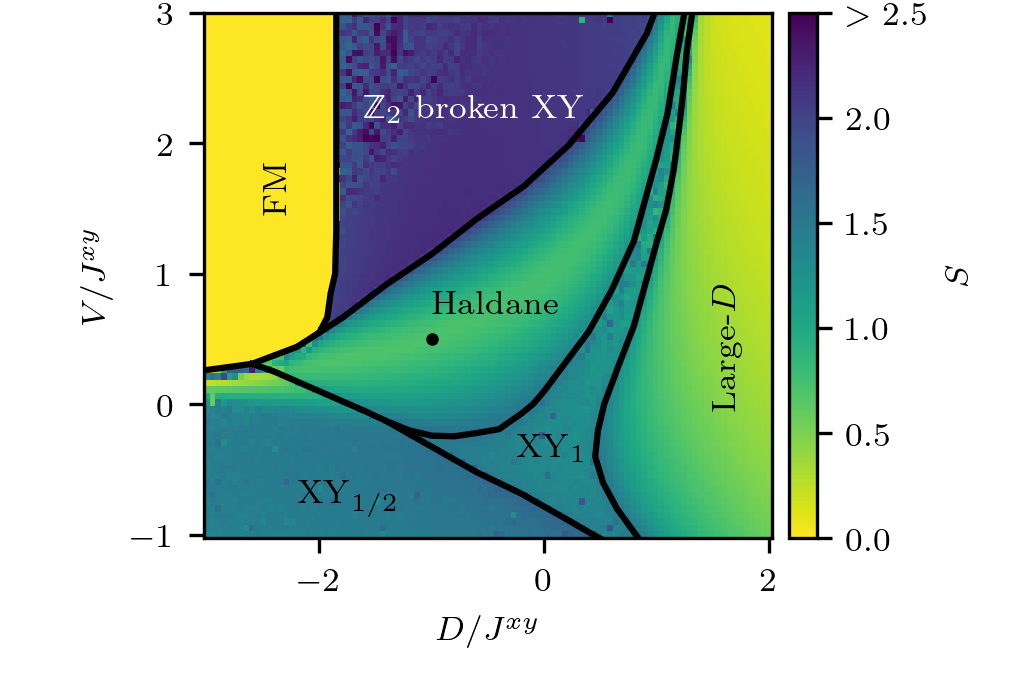
Figure 3: Phase diagram of our model [see eq. 1], calculated by using infinite DMRG within the TeNPy library [35] and a bond dimension of $\chi=400$. The color indicates the entanglement entropy $S$ of the ground state and is meant as a qualitative measure of the different phases, where local maxima indicate phase transitions. The solid lines are guide for the eyes and do not represent the exact phase transitions. For trivial product states the entropy is zero, while for gapless phases the entropy would diverge for increasing bond dimensions. Inside the Haldane phase one can see the entropy converging to a value of about $\log 2\approx 0.69$, corresponding to cutting one singlet bond of the AKLT state.

We choose $J^{xy}$ as energy scale. Thus, we are left with two degrees of freedom and can plot the phase diagram of the Hamiltonian (1) over $D$ and $V$. By plotting the entanglement entropy $S$, as shown in fig. 3, we can identify all occurring phase transitions (the solid lines are guide for the eyes and not exact phase transitions). To specify and characterize the different phases, we also examined other properties, such as string order parameters and the projective representation of the symmetries, which are discussed in detail in appendix B. The phase diagram was calculated using infinite DMRG within the TeNPy library [35]. Before we focus on the Haldane phase, let us briefly discuss the other phases in the phase diagram.

In the case of large positive values of $D$, we are in a gapped phase with a unique ground state (Large-$D$ phase). For $D\to\infty$, the ground state is a simple product state of all spins in the $\ket{0}$ state, thus the phase is a topological trivial phase. The ground state is disordered and invariant under the $D_{2}$ and time reversal symmetry.

Next, we consider the case of large negative values of $D\to-\infty$. In this case, the $\ket{0}$ state has a large energy penalty and effectively gets frozen out, such that the Hamiltonian reduces to a two-level Hamiltonian

$$H_{\text{effective}}=\sum_{i>j}\frac{V}{r_{ij}^{6}}\left(\sigma^{+}_{i}\sigma^{-}_{j}+\sigma^{-}_{i}\sigma^{+}_{j}\right)-\frac{V}{2r_{ij}^{6}}\sigma^{z}_{i}\sigma^{z}_{j}\ \,,$$ (5)

with $\sigma^{\pm}=\ket{\pm}\!\bra{\mp}$ and $\sigma^{z}=\ket{+}\!\bra{+}-\ket{-}\!\bra{-}$. This is the well known spin-$1/2$ XXZ model, but with finite range interactions $\propto r_{ij}^{-6}$. For negative values of $V$ we are in the gapless spin-1$/$2 ferromagnetic XY phase (XY_1/2) [36], where the low energy excitations are given by the Goldstone modes. The ground state exhibits quasi-long range order, i.e. the off-diagonal order parameter $\langle\sigma^{+}_{i}\sigma^{-}_{j}\rangle=\frac{1}{4}\langle(S^{+}_{i})^{2}(S^{-}_{j})^{2}\rangle$ decays algebraically with the distance $r_{ij}$. In the same limit of large negative $D$ but for positive values of $V$, we are in the gapped Ising ferromagnetic phase (FM). In the whole phase the two degenerate ground states are simple product states of all spins in the $\ket{+}$ or $\ket{-}$ state. It is a symmetry-broken phase and can easily be characterized by the Ising ferromagnetic long range order $\langle S^{z}_{i}S^{z}_{j}\rangle$.

Now we examine the spin-1 antiferromagnetic XY phase (XY₁), which, similarly to the XY_1/2 phase, is a gapless phase. The ground state also exhibits quasi-long range order, but now for both off-diagonal order parameters $\langle(-1)^{i-j}S^{+}_{i}S^{-}_{j}\rangle$ and $\langle(S^{+}_{i})^{2}(S^{-}_{j})^{2}\rangle$, which decay algebraically with the distance $r_{ij}$. Because the phase transition from the XY₁ phase to the Haldane phase is a BKT transition [37, 38, 33], it is hard to determine the exact boundaries from the correlation functions [39]. To get the precise BKT boundaries one can either use bond dimension scaling and very large distances utilizing the infinite DMRG algorithm [39, 34]. Alternatively, one can do finite size scaling as described in [40, 33].

For large positive values of $V$ we are again in a gapless phase. The ground state breaks the $\mathbb{Z}_{2}$ symmetry ($\pi$ rotation around the $x$-axis) of the Hamiltonian, which can be seen in DMRG by adding a small effective magnetic field $\sum_{i}S^{z}_{i}$. Furthermore, the ground state exhibits quasi-long range order in the off-diagonal order parameter $\langle(-1)^{i-j}S^{+}_{i}S^{-}_{j}\rangle$. Thus, we call this phase a $\mathbb{Z}_{2}$ broken antiferromagnetic XY phase.

We now focus on the Haldane phase in the middle of the phase diagram. It is a gapped phase with no long range order but finite string order parameters. The string order parameter is defined as

$$\mathcal{S}_{i,j}^{\alpha}=-\bra{\psi}S^{\alpha}_{i}\left(\prod_{k=i+1}^{j-1}(-1)^{S^{\alpha}_{k}}\right)S^{\alpha}_{j}\ket{\psi}\,,$$ (6)

and is a measure for the hidden antiferromagnetic order in the Haldane phase. At the marked point, all three string order parameters $\mathcal{S}_{0,500}^{x,y,z}$ are larger than $0.4$ (note that for the perfect AKLT state $\mathcal{S}_{1,\infty}^{x,y,z}=4/9$). In addition to the string order parameters, we characterized the Haldane phase using the degenerate entanglement spectrum [32] and the invariance of the infinite MPS under the $D_{2}$ and time reversal symmetries, which exhibit non-trivial phase factors in their projective representations [41]. We also verified a significant overlap with the perfect AKLT state. For more details on the phase diagram and the properties of the Haldane phase see appendix B.

From now on, we focus on the point $D=-J^{xy}$ and $V=0.6J^{xy}$, which is marked in fig. 3 by a black dot and lies inside the Haldane phase.

IV Experimental proposal

In this section, we propose a concrete example of experimental parameters that results in the desired values for $D$ and $V$. We discuss the Haldane phase in more detail within this experimental setup, including finite size results, possible detection schemes, and a potential ground state preparation scheme.

In section II, we discussed that the parameters $D$ and $V$ can be tuned in a Rydberg system by the experimental parameters. We propose to use the states defined in eq. 2 with a principal quantum number $n=80$ (and $81$ for the $\ket{+}$ state), an interatomic distance of $R=11.6\,\mathrm{\mu m}$ and a magnetic field of strength $B=60.7\,\mathrm{G}$, which is aligned at an angle of $\theta=35.1\,\mathrm{{}^{\circ}}$ with respect to the interatomic axis. The electric field is kept at $0$. Those parameters result in an anisotropy energy of $D/h=-4.47\,\mathrm{MHz}$ and nearest-neighbor ($nn$) interaction strengths of $J^{xy}_{nn}/h=4.47\,\mathrm{MHz}$ and $V_{nn}/h=2.68\,\mathrm{MHz}$. This corresponds to the point $D=-J^{xy}_{nn}$ and $V_{nn}=0.6J^{xy}_{nn}$, which we motivated in the last section. By also looking at further neighbor values, see appendix C for a full list of all interaction strengths, we find that the interaction strengths decay with $1/r_{ij}^{\alpha}$, where $\alpha\approx 3$ for dipolar interactions and $\alpha\approx 6$ for the van der Waals interactions, as predicted in section II.

Note two differences with respect to the simplified model we introduced in section II and discussed in section III. First, the couplings $J^{+0}_{nn}/h=4.36\,\mathrm{MHz}$ and $J^{-0}_{nn}/h=4.59\,\mathrm{MHz}$ are not exactly the same anymore. Second, there are now other additional van der Waals terms, see appendix C for more details. Both these effects result in a small symmetry breaking of the $D_{2}$ and time reversal symmetry, which however is only of the order of $0.03J^{xy}_{nn}$ and thus results in a small splitting of the four ground states of the Haldane phase. In the following, we always consider the full Hamiltonian including all terms listed in appendix C.

Let us now investigate an experimentally realizable finite size system with these parameters and discuss possibilities to measure the Haldane phase and its properties in an experiment. We use a system size of $L=10$ atoms, which already is enough to clearly see the separated edge states of the Haldane phase. However, all results in this section also generalize to larger system sizes. As expected, we do find four ground states with total magnetizations $M_{\mathrm{tot}}=-1,0,0,+1$ and a gap above the ground state manifold to the excited states of about $\sim 600\,\mathrm{kHz}$. The ground state manifold is split by a small amount of $\sim\pm 70\,\mathrm{kHz}$, which can be explained by the symmetry breaking terms in the Hamiltonian.

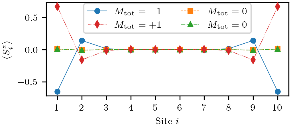
Figure 4: The expectation value of the local magnetization at each site for the four different ground states. For the $M_{\mathrm{tot}}=\pm 1$ states we can clearly see that the magnetization is localized at the edges. For the two degenerate $M_{\mathrm{tot}}=0$ states the edge states hybridize due to the small system size. Nevertheless, for all four ground states the edge spin correlation is non-zero $\left|\left\langle S^{z}_{1}S^{z}_{10}\right\rangle\right|\approx 0.4$, while it vanishes in the bulk $\left|\left\langle S^{z}_{1}S^{z}_{6}\right\rangle\right|\approx 0$. This reveals the edge states for all four ground states.

Looking at the site-resolved magnetization of the four different ground states in fig. 4, we see the fractional edge magnetization. Note that, even for this small system size, the edge states are already well separated from each other and, when summing over the magnetization of the 3 sites closest to the edge, we get values of almost exactly $\pm 0.5$.

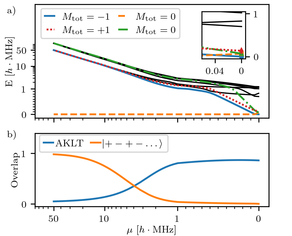
Figure 5: Adiabatic preparation scheme on a symlog scale (i.e. linear from $0$ to $1$ and logarithmic for the rest). a) The energy spectrum of the ten lowest eigenstates is shown for the sweep process. The sweep starts with a unique ground state and ends up with the fourfold near-degenerate ground state manifold of the Haldane phase. The four colored states correspond to the states ending in the ground state manifold of the final Hamiltonian. All other states are well separated from the ground state during the entire sweep by a gap of at least $600\,\mathrm{kHz}$. The inset shows the energy splitting of the ground state manifold at the end of the sweep. b) The overlap $\left|\braket{\Psi_{\mathrm{GS}}}{\Phi}\right|^{2}$ of the instantaneous ground state during the sweep with the product state $\ket{+-+-+-\dots}$ and the AKLT state $(\uparrow,\downarrow)$.

We now discuss a method to prepare these ground states of the Haldane phase by adiabatically sweeping from a product state to the desired ground state. An intuitive approach using a homogenous effective magnetic field as well as a Rabi frequency was already experimentally demonstrated for the SSH chain [14]. However, as we outline in appendix D, this method does not work for the AKLT state and our system. Here, we propose a different adiabatic preparation scheme only using a staggered, effective magnetic field.

We start with the initial state in a product state $\ket{+-+-+-\dots}$, which can be prepared by applying spatially dependent light shifts on the Rydberg chain [42]. By adding a strong staggered, effective magnetic field $\mu\sum_{i=1}^{L}(-1)^{i}S^{z}_{i}$ to the Hamiltonian, we ensure that this staggered state is initially the ground state of the system. Now, continuously turning off this staggered, effective magnetic field $\mu$, we end up with the desired Hamiltonian. As shown in fig. 5 a), the ground state manifold during this sweep is always well separated from the excited states by a gap of about $600\,\mathrm{kHz}$. We also numerically checked that the energy gap does not dependent on the system size. This allows us to adiabatically sweep from the product state to the Haldane phase, while never going through a gap closing. In fig. 5 b), we plotted the overlap of the instantaneous ground state with the product state $\ket{+-+-+-\dots}$ and the AKLT states during the preparation sweep. As described above, the initial ground state has a large overlap with the product state, while the final state has a large overlap with the AKLT state.

The Hamiltonian during the whole sweep conserves the total magnetization $M_{\mathrm{tot}}$. This allows us to also prepare the ground states with $M_{\mathrm{tot}}=\pm 1$ by using odd system sizes and a product state $\ket{+-\dots-+}$ or $\ket{-+\dots+-}$.

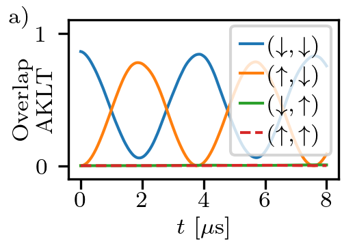
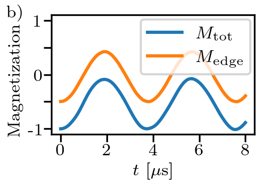
Figure 6: At time $t=0$ we start with the ground state of our Hamiltonian and apply a rotation around the $x$-axis on the first half of the chain for a time $t$. The Rabi frequency is $\Omega/h=0.25\,\mathrm{MHz}$, which results in a $\pi$ rotation after $2\,\mathrm{\mu s}$. a) The overlap of the time evolved state with the four different AKLT states, which are labelled according to their edge degrees of freedom. b) The magnetization of the full system $M_{\mathrm{tot}}=\left\langle\sum_{i=1}^{10}S^{z}_{i}\right\rangle$ and of the 3 leftmost edge sites $M_{\mathrm{edge}}=\left\langle\sum_{i=1}^{3}S^{z}_{i}\right\rangle$.

After preparing the ground state of the Haldane phase, one can now measure the ground state properties of the Haldane phase. These include the site-resolved magnetization shown in fig. 4, where the edge states can be seen. Furthermore, one can also measure the string order parameters, which were defined in eq. 6. For this finite size system the string order parameters of the ground state are $\mathcal{S}_{3,8}^{z}=0.29$ and $\mathcal{S}_{3,8}^{x}=0.49$, showing the strong hidden antiferromagnetic order of the system.

While some features of the edge states can be seen in the static expectation values of the ground state magnetization, we also investigate the dynamics of these edge states. This allows us to see the fractionalization of the spin-1 chain to spin-$1/2$ degrees of freedom at the edges. We start in the ground state with total magnetization $M_{\mathrm{tot}}=-1$. Then, we coherently drive the system between two different ground states by applying a microwave pulse with frequency $\omega=(E_{+}-E_{-})/2$ only to the left half of the chain. This drives both the transitions $\ket{+}\leftrightarrow\ket{0}$ and $\ket{-}\leftrightarrow\ket{0}$. In spin language this corresponds to the $S^{x}$ operator, which generates rotations around the $x$-axis. By using a Rabi frequency $\Omega$, which is small compared to the energy gap of the system, we ensure that the system is driven adiabatically and always stays inside the ground state manifold.

We now look at the time evolved state after some time $t$. As shown in fig. 6 a), the state oscillates between the two AKLT states with the spin-$1/2$ degree of freedom on the left edge pointing down or up. These oscillations correspond to Rabi oscillations of the fractionalized spin-$1/2$ degree of freedom at the left edge. One can also observe this in an experiment by measuring the expectation value of the magnetization at the 3 leftmost sites. As shown in fig. 6 b), the edge magnetization in $z$ direction oscillates between $-0.5$ and $+0.5$.

Additionally, in fig. 6 b), the total magnetization is plotted, showing oscillations between $-1$ and $0$. This indicates that after an effective $\pi$ rotation (i.e., after $2\,\mathrm{\mu s}$ for a microwave pulse with $\Omega=0.25\,\mathrm{MHz}$) of half the spin-1 chain, the total magnetization of the system changes from $-1$ to $0$. This is a clear signature of the fractionalization of the spin-1 chain into effective spin-$1/2$ edge states. In contrast, applying a $\pi$ rotation to a single spin-1 degree of freedom would only change the magnetization by $0$ or $\pm 2$ (since $\exp(i\pi S^{x})\ket{0}=-\ket{0}$ and $\exp(i\pi S^{x})\ket{\pm}=\ket{\mp}$). Importantly, when driving the system adiabatically (i.e., with a Rabi frequency $\Omega$ small compared to the gap), the state after the $\pi$ rotation remains an eigenstate of the total magnetization.

V Conclusion and Outlook

In this work we proposed a new way of using Förster resonances in Rydberg atoms to implement effective spin-1 systems with highly tunable interactions. The phase diagram of this Hamiltonian exhibits a large and stable region with the Haldane phase, which is characterized by a hidden antiferromagnetic order and fractionalized edge states. The aforementioned Haldane phase can be realized in Rydberg systems with an experimental setup and magnetic field strengths that are well within the possibilities of today existing experiments. In addition, we discussed an adiabatic available preparation scheme utilizing experimental techniques to prepare the Haldane phase. Finally, we studied a finite size realization of such Rydberg chains and proposed multiple ways of measuring the edge state features of the Haldane phase, including the fractionalization of these edge states. Therefore, we have laid out a complete path for implementing, preparing, and measuring the spin-1 Haldane phase in Rydberg platforms. Our detailed proposal should pave the way for experiments to study the spin-1 Haldane phase, and thus allows to detect and study the fractionalization of edge spin degrees of freedom.

Appendix A Mapping of Rydberg interactions to Spin-1 operators

In section II, we discussed the Rydberg energies and interactions in our model, which are again summarized here

$$H^{D}_{i} =D\left(\ket{+}\!\bra{+}+\ket{-}\!\bra{-}\right)\,,$$

$$H^{\mathrm{XY}}_{ij} =\Bigl{[}J^{+0}\ket{0+}\!\bra{+0}+J^{-0}\ket{-0}\!\bra{0-}$$

$$\quad\quad+J^{00}\left(\ket{-+}\!\bra{00}+\ket{+-}\!\bra{00}\right)\Bigr{]}+\text{h.c.}\,,$$

$$H^{\mathrm{V}}_{ij} =V^{\text{offd}}\left(\ket{+-}\!\bra{-+}+\ket{-+}\!\bra{+-}\right)$$

$$\quad\quad+V^{\text{diag}}\left(\ket{+-}\!\bra{+-}+\ket{-+}\!\bra{-+}\right)\,.$$ (7)

Note that the anisotropy term $H^{D}_{i}$ is due to the Förster resonance offset of the state $\ket{00}$ relative to the state $\ket{+-}$ and up to a global energy shift we could also write it in the more intuitive form $H^{D}_{i}=-D\ket{0}\!\bra{0}$.

Here, we map these Rydberg interactions to spin-1 interactions and the spin-1 algebra. The spin-1 operators in the eigenbasis of $S^{z}$, i.e. $\ket{+}$, $\ket{0}$ and $\ket{-}$, are given as

$$S^{x} =\frac{1}{\sqrt{2}}\begin{pmatrix}0&1&0\\ 1&0&1\\ 0&1&0\end{pmatrix}\,,S^{y}=\frac{1}{\sqrt{2}}\begin{pmatrix}0&-i&0\\ i&0&-i\\ 0&i&0\end{pmatrix}\,,$$

$$S^{z} =\begin{pmatrix}1&0&0\\ 0&0&0\\ 0&0&-1\end{pmatrix}\,\text{ and }S^{\pm}=S^{x}\pm iS^{y}\,.$$ (8)

One can easily see that the anisotropy term simply maps to $H^{D}_{i}=D(S^{z}_{i})^{2}$.

As discussed in section II, the dipole-dipole interactions can be tuned to be approximately the same: $J^{+0}=J^{-0}=J^{00}\equiv J^{xy}$. This simplifies the expression, since $H^{\mathrm{XY}}_{ij}$ now simply involves all total spin conserving interactions, which change the spin of each individual site by $\pm 1$. One can quickly convince oneself that this corresponds to the following spin-1 XY interactions

$$H^{\mathrm{XY}}_{ij}=\frac{J^{xy}}{2}\left(S^{+}_{i}S^{-}_{j}+S^{-}_{i}S^{+}_{j}\right)=J^{xy}\left(S^{x}_{i}S^{x}_{j}+S^{y}_{i}S^{y}_{j}\right)\,.$$ (9)

For the van der Waals term we first look at the off-diagonal elements $\ket{+-}\!\bra{-+}+\ket{-+}\!\bra{+-}$. These are total spin conserving interactions, which change the spin magnetization of each individual site by $\pm 2$. We therefore can describe this term by $(S^{+}_{i})^{2}(S^{-}_{j})^{2}+(S^{-}_{i})^{2}(S^{+}_{j})^{2}$. The diagonal elements only act on states if neither of them is $\ket{0}$ leading to $S^{z}_{i}S^{z}_{j}$, and they have not the same magnetization, which can be enforced by $(S^{z}_{i}S^{z}_{j}-1)$. Including the correct prefactors we thus end up with

$$H^{\mathrm{V}}_{ij} =\frac{V^{\text{offd}}}{4}\left((S^{+}_{i})^{2}(S^{-}_{j})^{2}+(S^{-}_{i})^{2}(S^{+}_{j})^{2}\right)$$

$$\quad+\frac{V^{\text{diag}}}{2}S^{z}_{i}S^{z}_{j}(S^{z}_{i}S^{z}_{j}-1)\,.$$ (10)

Appendix B More details on the phase diagram

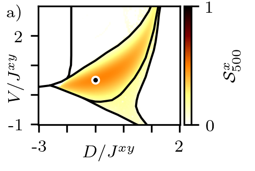
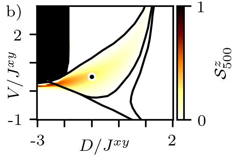
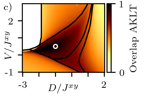
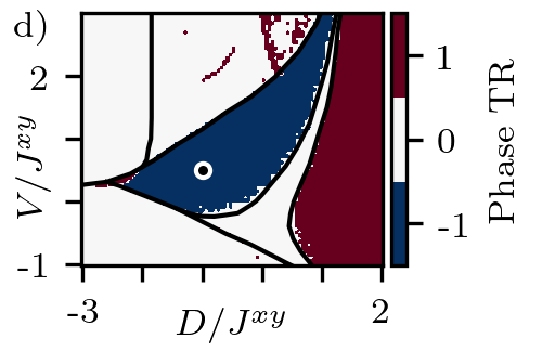
Figure 7: The same phase diagram as discussed in section III but now showing a) and b) the $x$ and $z$ string order parameter c) the overlap of the ground state with the perfect AKLT state d) the phase factor of the projective representation of the time reversal symmetry. All plots have a resolution of $100\times 100$ points.

In this section we elaborate on the phase diagram discussed in section III, see also [27]. Specifically we discuss the properties of the Haldane phase that can be used to numerically distinguish it from the other phases.

In fig. 7 a) and b), we plotted the string order parameters $\mathcal{S}_{0,500}^{x}$ and $\mathcal{S}_{0,500}^{z}$ for two spins separated by $500$ sites. The $x$ string order parameter has a finite value in the whole Haldane phase as well as a smaller but finite value also in the XY₁ phase, which is due to the finite separation and finite bond dimensions and the small decay of the $x$ string order parameter in the XY₁ phase (for more details about this see [39]). The $z$ string order parameter is perfectly $1$ in the ferromagnetic phase and apart from that only has finite values inside the Haldane phase. However, it gets smaller the closer we get to any phase transition.

Next, in fig. 7 c), we have plotted the largest eigenvalue of the transfer matrix of the contraction of the perfect AKLT unit cell and the unit cell of the infinite MPS ground state, where the unit cells consisted of two single sites. This effectively describes an overlap of the ground state with the AKLT state per unit cell (for an infinite system). One can see that this overlap peeks inside the Haldane phase and reaches values close to $1$, thus letting us conclude that the ground state is indeed very close to the AKLT state.

Finally, in fig. 7 d), we plotted the phase factor of the projective representation of the time reversal (TR) symmetry. This is defined to be $0$ where the ground state is not invariant under time reversal and otherwise reflects the phase factor of the projective representation of the time reversal symmetry group on the infinite MPS if the state is invariant (for more details on this see [41]). We can see that the Large-$D$ phase is a symmetric, but topologically trivial phase (i.e. phase factor of $+1$) under time reversal. On the other hand, the ground state in the Haldane phase is also invariant under time reversal, but has a non-trivial phase factor $-1$ and thus corresponds to the topological counterpart of the symmetric Large-$D$ phase.

Appendix C Full experimental Rydberg Hamiltonian

For the full experimental Hamiltonian we consider pairs of Rydberg atoms with distances ranging from nearest neighbors ($R=11.6\,\mathrm{\mu m}$) up to fifth-nearest neighbors ($R=58.0\,\mathrm{\mu m}$). For each pair we use the pairinteraction software [31] to calculate an effective interaction Hamiltonian for the nine pair states of interest ($\ket{++}$, $\ket{+0}$, $\dots$, $\ket{--}$). This is done by first considering the single Rydberg atoms and taking into account all states close to the $80S$, $80P$ and $81S$ manifolds (i.e. states within an energy window of $\pm 80\,\mathrm{GHz}$, a principal quantum number $76\leq n\leq 85$ and an azimuthal quantum number $l\leq 4$). We then use the eigenstates of the single atom Hamiltonian (including the magnetic field) to construct a pair Hamiltonian. However, we restrict the basis of the pair Hamiltonian to only pair states within an energy window of $\pm 2\,\mathrm{GHz}$ around the five different subspaces of pair magnetization $M_{\text{pair}}=\pm 2,\pm 1,0$, since the effect of states further away is negligible. This already results in up to $\sim 5000$ pair states that we need to consider for each subspace. Finally, we apply a direct rotation that maps the pair Hamiltonian to the subspace of interest and thus obtain an effective interaction Hamiltonian [43]. Combining the 5 subspaces to a full Hamiltonian we then obtain a $9\times 9$ interaction matrix for each pair of the following structure

$$H_{ij}=\begin{pmatrix}V^{++}_{ij}&&&&&&&&\\ &V^{+0}_{ij}&&J^{+0}_{ij}&&&&&\\ &&V^{\text{diag}}_{ij}&&J^{00}_{ij}&&V^{\text{offd}}_{ij}&&\\ &J^{+0}_{ij}&&V^{+0}_{ij}&&&&&\\ &&J^{00}_{ij}&&V^{00}_{ij}&&J^{00}_{ij}&&\\ &&&&&V^{-0}_{ij}&&J^{-0}_{ij}&\\ &&V^{\text{offd}}_{ij}&&J^{00}_{ij}&&V^{\text{diag}}_{ij}&&\\ &&&&&J^{-0}_{ij}&&V^{-0}_{ij}&\\ &&&&&&&&V^{--}_{ij}\end{pmatrix}\,.$$ (11)

The interaction strengths for the parameters defined in section IV for each pair up to a distance of 5 sites are listed in the following table 1. Note that values smaller than $0.01\,\mathrm{MHz}$ are not listed (for $V^{00}$ this is true even for nearest neighbors).

Table 1: Interaction strengths for the Rydberg Hamiltonian (12) in $\mathrm{h\cdot\mathrm{MHz}}$.

$\left|i-j\right|$	1	2	3	4	5
$J^{+0}_{ij}/h$	4.36	0.56	0.17	0.07	0.04
$J^{-0}_{ij}/h$	4.59	0.59	0.17	0.07	0.04
$J^{00}_{ij}/h$	4.46	0.57	0.17	0.07	0.04
$V^{\text{diag}}_{ij}/h$	2.99	0.05
$V^{\text{offd}}_{ij}/h$	2.38	0.04
$V^{+0}_{ij}/h$	1.10	0.02
$V^{-0}_{ij}/h$	1.10	0.02
$V^{++}_{ij}/h$	1.84	0.03
$V^{--}_{ij}/h$	2.13	0.03

The anisotropy energy $D$ is simply given by half the energy difference between the $\ket{+-}$ and $\ket{00}$ states and for the parameters given in section IV is $D/h=-4.47\,\mathrm{MHz}$. The full many-body Hamiltonian can then be written as

$$H =\sum_{i<j}H_{ij}+D\sum_{i}\left(S^{z}_{i}\right)^{2}\,.$$ (12)

Appendix D Details on the preparation scheme

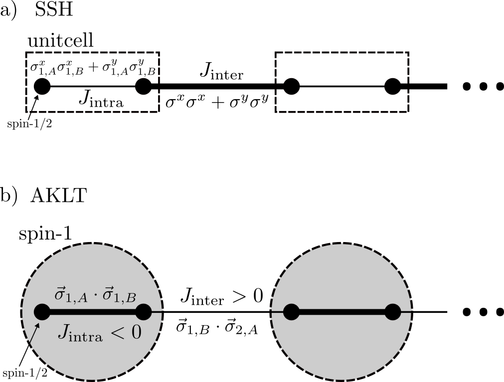
Figure 8: Sketch of the SSH and AKLT model with their typical interactions, where thick lines indicate strong couplings. a) The SSH model with strong inter-cell XY couplings and weak intra-cell XY couplings, where each unit-cell consists of two spin-$1/2$ particles. b) The AKLT model, where each spin-1 particle can be thought of as a pair of strongly ferromagnetic coupled virtual spin-$1/2$ particles. In this picture the AKLT interactions correspond to isotropic, antiferromagnetic couplings between those virtual spin-$1/2$ particles of neighboring spin-1 particles.

In this section we review a different adiabatic preparation scheme for the SSH chain, which was already successfully realized in a system of Rydberg atoms [14]. We discuss how this scheme changes when considering an antiferromagnetic SSH chain instead of the ferromagnetic one (similar differences for the ferromagnetic and antiferromagnetic case have also been discussed for preparing 2d XY magnets [42]). We then connect the antiferromagnetic SSH chain to the AKLT model and discuss the adapted preparation scheme in the context of the AKLT model. By doing so we motivate the preparation scheme proposed in section IV, which only uses a staggered, effective magnetic field.

The periodic SSH Hamiltonian is defined as

$$H_{\mathrm{SSH}} =\sum_{i=1}^{L}J_{\mathrm{intra}}\left(\sigma^{x}_{i,A}\sigma^{x}_{i,B}+\sigma^{y}_{i,A}\sigma^{y}_{i,B}+\delta\sigma^{z}_{i,A}\sigma^{z}_{i,B}\right)$$

$$+\sum_{i=1}^{L}J_{\mathrm{inter}}\left(\sigma^{x}_{i,B}\sigma^{x}_{i+1,A}+\sigma^{y}_{i,B}\sigma^{y}_{i+1,A}+\delta\sigma^{z}_{i,B}\sigma^{z}_{i+1,A}\right)\,,$$ (13)

where $\sigma^{\alpha}_{L+1,A}=\sigma^{\alpha}_{1,A}$. $J_{\mathrm{intra}}$ describes the coupling within one unit cell between the sites $A$ and $B$, and $J_{\mathrm{inter}}$ describes the coupling of site $B$ and site $A$ between two neighboring unit cells. $\delta$ is an anisotropy parameter and only used for connecting the SSH Hamiltonian to the AKLT Hamiltonian. For the SSH chain the inter-cell coupling is typically stronger than the intra-cell coupling, i.e. $\left|J_{\mathrm{inter}}\right|>\left|J_{\mathrm{intra}}\right|$. These interactions are also sketched in fig. 8 a), where thick lines indicate strong couplings.

We first consider the ferromagnetic case $J_{\mathrm{inter}}<0$ with $\left|J_{\mathrm{intra}}\right|\ll\left|J_{\mathrm{inter}}\right|$ and $\delta=0$ (this is similar to the SSH model used in [14]). This corresponds to strong ferromagnetic inter-cell couplings, which ground state can be described in the limit of $J_{\mathrm{intra}}\to 0$ by a product of neighboring triplet states

$$\ket{\psi_{\mathrm{SSH,ferro}}}\approx\prod_{i=1}^{L}\frac{1}{\sqrt{2}}\left(\ket{\uparrow}_{i,B}\ket{\downarrow}_{i+1,A}+\ket{\downarrow}_{i,B}\ket{\uparrow}_{i+1,A}\right)\,.$$ (14)

The crucial step to adiabatically prepare this state is to have in addition to the SSH Hamiltonian a strong, homogenous microwave field $-\Omega\sum_{i,a\in\{A,B\}}\sigma^{x}_{i,a}$, for which the ground state is a simple product state $\ket{\Phi_{\mathrm{homog}}}=\prod_{i,a\in\{A,B\}}\ket{\rightarrow}_{i,a}$, where $\ket{\rightarrow}=\frac{1}{\sqrt{2}}\left(\ket{\uparrow}+\ket{\downarrow}\right)$. Then, slowly turning the microwave field off yields the desired SSH ground state. Note that the product state $\ket{\Phi_{\mathrm{homog}}}$ has a large overlap with the ferromagnetic SSH ground state $\ket{\psi_{\mathrm{SSH,ferro}}}$, which is an intuitive way to explain why during this preparation scheme no gap closing occurs.

Secondly we consider the antiferromagnetic case $J_{\mathrm{inter}}>0$, again with $\left|J_{\mathrm{intra}}\right|\ll\left|J_{\mathrm{inter}}\right|$ and $\delta=0$. The ground state for these strong antiferromagnetic inter-cell couplings in the limit of $J_{\mathrm{intra}}\to 0$ is given by the product state of neighboring singlet states

$$\ket{\psi_{\mathrm{SSH,antiferro}}}\approx\prod_{i=1}^{L}\frac{1}{\sqrt{2}}\left(\ket{\uparrow}_{i,B}\ket{\downarrow}_{i+1,A}-\ket{\downarrow}_{i,B}\ket{\uparrow}_{i+1,A}\right)\,.$$ (15)

Contrary to the ferromagnetic case, the overlap of this antiferromagnetic SSH ground state with the product state $\ket{\Phi_{\mathrm{homog}}}$ is zero. And indeed, checking the energy spectrum of the Hamiltonian when turning off the homogenous microwave field $\Omega$, we find a gap-closing point during the sweep.

Notice, however, that the antiferromagnetic SSH Hamiltonian can be obtained from the ferromagnetic SSH Hamiltonian by rotating all spins of the sublattice $B$ by $\pi$ around the $z$-axis. Thus, we can instead also switch the sign of the microwave field for the sublattice $B$ resulting in a staggered microwave field. The initial state for this staggered microwave field is then also a product state $\ket{\Phi_{\mathrm{staggered}}}=\prod_{i}\ket{\rightarrow}_{i,A}\ket{\leftarrow}_{i,B}$, where $\ket{\leftarrow}=\frac{1}{\sqrt{2}}\left(\ket{\uparrow}-\ket{\downarrow}\right)$. This state again has a large overlap with the antiferromagnetic SSH ground state $\ket{\psi_{\mathrm{SSH,antiferro}}}$ and allows for a gapless preparation path.

Now we relate the antiferromagnetic SSH spin-$1/2$ chain to the spin-1 AKLT model. Adding $\delta=1$ to the antiferromagnetic SSH Hamiltonian and a strong ferromagnetic intra-cell coupling $-J_{\mathrm{intra}}\gg J_{\mathrm{inter}}$, we can connect the SSH Hamiltonian to the AKLT Hamiltonian along a gapped path (see appendix of [14] for more details). The AKLT Hamiltonian is given by

$$H_{\mathrm{AKLT}} =\sum_{i=1}^{L}P^{S=2}_{i,i+1}$$ (16)

$$\sim\sum_{i=1}^{L}J_{\mathrm{intra}}\vec{\sigma}_{i,A}\vec{\sigma}_{i,B}+J_{\mathrm{inter}}\vec{\sigma}_{i,B}\vec{\sigma}_{i+1,A}\,,$$ (17)

where $P^{S=2}_{i,i+1}$ is the projector of two neighboring spin-1 particles onto a spin-2 subspace. Here, the strong ferromagnetic intra-cell coupling $J_{\mathrm{intra}}<0$ of two spin-$1/2$ particles inside one unit cell projects each unit cell effectively to a spin-1 particle, and the antiferromagnetic inter-cell coupling $J_{\mathrm{inter}}>0$ enforces the typical singlet bonds of the AKLT state between neighboring unit cells. This is also shown in fig. 8 b), where the strong couplings (represented by thick lines) are now inside the unit cell.

With this in mind, we are no longer surprised that applying a homogenous microwave field to the AKLT model does not yield a gapped preparation path, since for the antiferromagnetic SSH model a homogenous microwave field also was not sufficient. Inspired by the staggered microwave field for the SSH chain one can also apply a staggered microwave field $\Omega\sum_{i}(-1)^{i}S^{x}_{i}$ to the AKLT model, where $S^{x}_{i}$ are now spin-1 operators. This indeed yields a gapped preparation path from a product state of spin-1 eigenstates of the $S^{x}_{i}$ operator to the AKLT state. Finally, since the AKLT Hamiltonian is $SO(3)$ invariant we can replace the staggered microwave field $\pm S^{x}$ by a staggered, effective magnetic field $\mu\sum_{i}(-1)^{i}S^{z}_{i}$. As shown in section IV, this staggered, effective magnetic field does also provide a gapped preparation path to the ground state of Haldane phase for our Rydberg model.

References

- Wen [2017] X.-G. Wen, Zoo of quantum-topological phases of matter, Reviews of Modern Physics 89, 041004 (2017).
- Stormer et al. [1999] H. L. Stormer, D. C. Tsui, and A. C. Gossard, The fractional quantum Hall effect, Reviews of Modern Physics 71, S298 (1999).
- Verresen et al. [2021] R. Verresen, M. D. Lukin, and A. Vishwanath, Prediction of Toric Code Topological Order from Rydberg Blockade, Physical Review X 11, 031005 (2021).
- Semeghini et al. [2021] G. Semeghini, H. Levine, A. Keesling, S. Ebadi, T. T. Wang, D. Bluvstein, R. Verresen, H. Pichler, M. Kalinowski, R. Samajdar, A. Omran, S. Sachdev, A. Vishwanath, M. Greiner, V. Vuletic, and M. D. Lukin, Probing Topological Spin Liquids on a Programmable Quantum Simulator, Science 374, 1242 (2021).
- Chen et al. [2011] X. Chen, Z.-C. Gu, and X.-G. Wen, Classification of gapped symmetric phases in one-dimensional spin systems, Physical Review B 83, 035107 (2011).
- Haldane [1983a] F. D. M. Haldane, Nonlinear Field Theory of Large-Spin Heisenberg Antiferromagnets: Semiclassically Quantized Solitons of the One-Dimensional Easy-Axis Néel State, Physical Review Letters 50, 1153 (1983a).
- Haldane [1983b] F. D. M. Haldane, Continuum dynamics of the 1-D Heisenberg antiferromagnet: Identification with the O(3) nonlinear sigma model, Physics Letters A 93, 464 (1983b).
- Affleck et al. [1987] I. Affleck, T. Kennedy, E. H. Lieb, and H. Tasaki, Rigorous results on valence-bond ground states in antiferromagnets, Physical Review Letters 59, 799 (1987).
- Altman et al. [2021] E. Altman, K. R. Brown, G. Carleo, L. D. Carr, E. Demler, C. Chin, B. DeMarco, S. E. Economou, M. A. Eriksson, K.-M. C. Fu, M. Greiner, K. R. Hazzard, R. G. Hulet, A. J. Kollár, B. L. Lev, M. D. Lukin, R. Ma, X. Mi, S. Misra, C. Monroe, K. Murch, Z. Nazario, K.-K. Ni, A. C. Potter, P. Roushan, M. Saffman, M. Schleier-Smith, I. Siddiqi, R. Simmonds, M. Singh, I. Spielman, K. Temme, D. S. Weiss, J. Vučković, V. Vuletić, J. Ye, and M. Zwierlein, Quantum Simulators: Architectures and Opportunities, PRX Quantum 2, 017003 (2021).
- Gross and Bloch [2017] C. Gross and I. Bloch, Quantum simulations with ultracold atoms in optical lattices, Science 357, 995 (2017).
- Monroe et al. [2021] C. Monroe, W. C. Campbell, L.-M. Duan, Z.-X. Gong, A. V. Gorshkov, P. W. Hess, R. Islam, K. Kim, N. M. Linke, G. Pagano, P. Richerme, C. Senko, and N. Y. Yao, Programmable quantum simulations of spin systems with trapped ions, Reviews of Modern Physics 93, 025001 (2021).
- Browaeys and Lahaye [2020] A. Browaeys and T. Lahaye, Many-Body Physics with Individually-Controlled Rydberg Atoms, Nature Physics 16, 132 (2020).
- Weber et al. [2018] S. Weber, S. de Léséleuc, V. Lienhard, D. Barredo, T. Lahaye, A. Browaeys, and H. P. Büchler, Topologically protected edge states in small Rydberg systems, Quantum Science and Technology 3, 044001 (2018).
- De Léséleuc et al. [2019] S. De Léséleuc, V. Lienhard, P. Scholl, D. Barredo, S. Weber, N. Lang, H. P. Büchler, T. Lahaye, and A. Browaeys, Observation of a symmetry-protected topological phase of interacting bosons with Rydberg atoms, Science 365, 775 (2019).
- Lienhard et al. [2020] V. Lienhard, P. Scholl, S. Weber, D. Barredo, S. de Léséleuc, R. Bai, N. Lang, M. Fleischhauer, H. P. Büchler, T. Lahaye, and A. Browaeys, Realization of a density-dependent Peierls phase in a synthetic, spin-orbit coupled Rydberg system, Physical Review X 10, 021031 (2020).
- Sørensen et al. [2005] A. S. Sørensen, E. Demler, and M. D. Lukin, Fractional Quantum Hall States of Atoms in Optical Lattices, Physical Review Letters 94, 086803 (2005).
- Büchler et al. [2005] H. P. Büchler, M. Hermele, S. D. Huber, M. P. A. Fisher, and P. Zoller, Atomic Quantum Simulator for Lattice Gauge Theories and Ring Exchange Models, Physical Review Letters 95, 040402 (2005).
- Duan et al. [2003] L.-M. Duan, E. Demler, and M. D. Lukin, Controlling Spin Exchange Interactions of Ultracold Atoms in Optical Lattices, Physical Review Letters 91, 090402 (2003).
- Miroshnychenko et al. [2006] Y. Miroshnychenko, W. Alt, I. Dotsenko, L. Förster, M. Khudaverdyan, A. Rauschenbeutel, and D. Meschede, Precision preparation of strings of trapped neutral atoms, New Journal of Physics 8, 191 (2006).
- Kim et al. [2016] H. Kim, W. Lee, H.-g. Lee, H. Jo, Y. Song, and J. Ahn, In situ single-atom array synthesis using dynamic holographic optical tweezers, Nature Communications 7, 13317 (2016).
- Endres et al. [2016] M. Endres, H. Bernien, A. Keesling, H. Levine, E. R. Anschuetz, A. Krajenbrink, C. Senko, V. Vuletic, M. Greiner, and M. D. Lukin, Atom-by-atom assembly of defect-free one-dimensional cold atom arrays, Science 354, 1024 (2016).
- Barredo et al. [2016] D. Barredo, S. de Léséleuc, V. Lienhard, T. Lahaye, and A. Browaeys, An atom-by-atom assembler of defect-free arbitrary two-dimensional atomic arrays, Science 354, 1021 (2016).
- Labuhn et al. [2016] H. Labuhn, D. Barredo, S. Ravets, S. de Léséleuc, T. Macrì, T. Lahaye, and A. Browaeys, Tunable two-dimensional arrays of single Rydberg atoms for realizing quantum Ising models, Nature 534, 667 (2016).
- Weber et al. [2022] S. Weber, R. Bai, N. Makki, J. Mögerle, T. Lahaye, A. Browaeys, M. Daghofer, N. Lang, and H. P. Büchler, Experimentally Accessible Scheme for a Fractional Chern Insulator in Rydberg Atoms, PRX Quantum 3, 030302 (2022).
- Safinya et al. [1981] K. A. Safinya, J. F. Delpech, F. Gounand, W. Sandner, and T. F. Gallagher, Resonant Rydberg-Atom-Rydberg-Atom Collisions, Physical Review Letters 47, 405 (1981).
- Ryabtsev et al. [2010] I. I. Ryabtsev, D. B. Tretyakov, I. I. Beterov, and V. M. Entin, Observation of the Stark-Tuned Förster Resonance between Two Rydberg Atoms, Physical Review Letters 104, 073003 (2010).
- Mögerle [2022] J. Mögerle, Spin 1 haldane phase in one-dimensional systems of rydberg atoms (2022), Master thesis, University of Stuttgart.
- Liu et al. [2024] V. S. Liu, M. Bintz, M. Block, R. Samajdar, J. Kemp, and N. Y. Yao, Supersolidity and Simplex Phases in Spin-1 Rydberg Atom Arrays (2024).
- Homeier et al. [2024] L. Homeier, T. J. Harris, T. Blatz, S. Geier, S. Hollerith, U. Schollwöck, F. Grusdt, and A. Bohrdt, Antiferromagnetic bosonic - models and their quantum simulation in tweezer arrays, Physical Review Letters 132, 230401 (2024).
- Sompet et al. [2022] P. Sompet, S. Hirthe, D. Bourgund, T. Chalopin, J. Bibo, J. Koepsell, P. Bojović, R. Verresen, F. Pollmann, G. Salomon, C. Gross, T. A. Hilker, and I. Bloch, Realising the Symmetry-Protected Haldane Phase in Fermi-Hubbard Ladders, Nature 606, 484 (2022).
- Weber et al. [2017] S. Weber, C. Tresp, H. Menke, A. Urvoy, O. Firstenberg, H. P. Büchler, and S. Hofferberth, Tutorial: Calculation of Rydberg interaction potentials, Journal of Physics B: Atomic, Molecular and Optical Physics 50, 133001 (2017).
- Pollmann et al. [2010] F. Pollmann, E. Berg, A. M. Turner, and M. Oshikawa, Entanglement spectrum of a topological phase in one dimension, Physical Review B 81, 064439 (2010).
- Chen et al. [2003] W. Chen, K. Hida, and B. C. Sanctuary, Ground-state phase diagram of S = 1 XXZ chains with uniaxial single-ion-type anisotropy, Physical Review B 67, 104401 (2003).
- Gong et al. [2016] Z.-X. Gong, M. F. Maghrebi, A. Hu, M. Foss-Feig, P. Richerme, C. Monroe, and A. V. Gorshkov, Kaleidoscope of quantum phases in a long-range interacting spin-1 chain, Physical Review B 93, 205115 (2016).
- Hauschild and Pollmann [2018] J. Hauschild and F. Pollmann, Efficient numerical simulations with Tensor Networks: Tensor Network Python (TeNPy), SciPost Physics Lecture Notes , 5 (2018).
- Peter et al. [2012] D. Peter, S. Müller, S. Wessel, and H. P. Büchler, Anomalous Behavior of Spin Systems with Dipolar Interactions, Physical Review Letters 109, 025303 (2012).
- Schulz [1986] H. J. Schulz, Phase diagrams and correlation exponents for quantum spin chains of arbitrary spin quantum number, Physical Review B 34, 6372 (1986).
- Kitazawa et al. [1996] A. Kitazawa, K. Nomura, and K. Okamoto, Phase Diagram of S = 1 Bond-Alternating XXZ Chains, Physical Review Letters 76, 4038 (1996).
- Heng Su et al. [2012] Y. Heng Su, S. Young Cho, B. Li, H.-L. Wang, and H.-Q. Zhou, Non-local Correlations in the Haldane Phase for an XXZ Spin-1 Chain: A Perspective from Infinite Matrix Product State Representation, Journal of the Physical Society of Japan 81, 074003 (2012).
- Kitazawa and Nomura [1997] A. Kitazawa and K. Nomura, Critical Properties of S = 1 Bond-Alternating XXZ Chains and Hidden Symmetry, Journal of the Physical Society of Japan 66, 3944 (1997).
- Pollmann and Turner [2012] F. Pollmann and A. M. Turner, Detection of Symmetry Protected Topological Phases in 1D, Physical Review B 86, 125441 (2012).
- Chen et al. [2023] C. Chen, G. Bornet, M. Bintz, G. Emperauger, L. Leclerc, V. S. Liu, P. Scholl, D. Barredo, J. Hauschild, S. Chatterjee, M. Schuler, A. M. Läuchli, M. P. Zaletel, T. Lahaye, N. Y. Yao, and A. Browaeys, Continuous symmetry breaking in a two-dimensional Rydberg array, Nature 616, 691 (2023).
- Bravyi et al. [2011] S. Bravyi, D. DiVincenzo, and D. Loss, Schrieffer-Wolff transformation for quantum many-body systems, Annals of Physics 326, 2793 (2011).