The more accurately we model the metal-dependent star formation rate, the larger the predicted excess of binary black hole mergers

As the number of gravitational-wave detections grows, the merger rate of binary black holes (BBHs) can help us to constrain their formation, the properties of their progenitors, and their birth environment. Here, we aim to address the impact of the metal-dependent star formation rate (SFR) on the BBH merger rate. To this end, we have developed a fully data-driven approach to model the metal-dependent SFR and coupled it to BBH evolution. We have adopted the most up-to-date scaling relations, based on recent observational results, and we have studied how the BBH merger rate density varies over a wide grid of galaxy and binary evolution parameters. Our results show that including a realistic metal-dependent SFR evolution yields a value of the merger rate density which is too high compared to the one inferred from GW data. Moreover, variations of the SFR in low-mass galaxies ($M_{\ast}\lesssim 10^{8}\mathrm{M}_{\odot}$) do not contribute more than a factor $\sim 2$ to the overall merger rate density at redshift $z=0$. These results suggest that the discrepancy between the BBH merger rate density inferred from data and theoretical models is not caused by approximations in the treatment of the metal-dependent SFR, but rather stems from stellar evolution models and/or BBH formation channels.

1 Introduction

The advent of gravitational wave (GW) detections has significantly expanded our understanding of stellar-mass black holes (BHs) and neutron stars (NSs, Abbott et al. 2016b, a, 2017b, 2017a, 2021, 2023a, 2024). LIGO–Virgo–KAGRA (LVK) data offers valuable insights into the mass function of binary BHs (BBHs), challenging existing stellar evolutionary models with observations of BHs within the lower and upper mass gaps (e.g. Abbott et al., 2023a, 2024). Moreover, as the dataset grows, a possible evolution of BBH properties with redshift $z$ is beginning to surface, even with current observations limited to $z\lesssim 1.5$ (Biscoveanu et al., 2022; Abbott et al., 2023b; Nitz et al., 2023; Ray et al., 2023; Callister & Farr, 2024; Rinaldi et al., 2024). Next-generation GW detectors will further advance our ability to explore the Universe, allowing us to probe BBH mergers at redshifts up to $z\lesssim 100$ (Hall & Evans, 2019; Kalogera et al., 2021; Branchesi et al., 2023). Specifically, the study of the BBH merger rates as a function of redshift can help us to test and distinguish among different formation channels of such objects (e.g. Belczynski et al., 2002; Dominik et al., 2013; Neijssel et al., 2019; Baibhav et al., 2019; Mapelli, 2020, 2021; Zevin et al., 2021; Broekgaarden et al., 2021; Mandel & Broekgaarden, 2022; Belczynski et al., 2022; van Son et al., 2022; Broekgaarden et al., 2022). The merger rate density is the result of the interplay between binary star evolution and the history of cosmic star formation (Lamberts et al., 2018; Santoliquido et al., 2020; Broekgaarden et al., 2021; Santoliquido et al., 2022; Boesky et al., 2024a, b; Chruślińska, 2024).

Most previous work relies on averaged star formation rate (SFR) density and metallicity distribution relations (e.g. van Son et al., 2022; Santoliquido et al., 2020; Neijssel et al., 2019). This assumption makes it extremely straightforward to calculate the merger rate density evolution, but contains several approximations in the description of the star formation process and metallicity evolution in the Universe. Such assumptions affect both the shape and absolute values of the estimated merger rates, as shown by several authors (Boco et al., 2019, 2021; Santoliquido et al., 2022; Briel et al., 2022). Emerging trends indicate that state-of-the-art population-synthesis models, when applied to more refined Universe models, yield BBH merger rates higher than those inferred by LVK (e.g. Santoliquido et al., 2022; Srinivasan et al., 2023; Boesky et al., 2024a).

This discrepancy is largely driven by the interplay of merger efficiency (i.e., the number of BHs that merge per total stellar mass) and metal-poor star formation (Belczynski et al., 2010; Mapelli et al., 2019; Chruslinska & Nelemans, 2019; Neijssel et al., 2019; Tang et al., 2020; Santoliquido et al., 2021; Broekgaarden et al., 2021; Chruślińska, 2024). In fact, the merger efficiency of BBHs is 1-4 orders of magnitude higher in metal-poor than in metal-rich progenitor systems (Klencki et al., 2018; Giacobbo & Mapelli, 2018; Spera et al., 2019; Broekgaarden et al., 2021; Iorio et al., 2023). Hence, the merger rate density evolution should be largely boosted by star formation in metal-poor regions, often associated with low-mass galaxies. As discussed by Chruślińska et al. (2021); Boco et al. (2021); Chruślińska (2024) the large uncertainties concerning the metallicity evolution in the Universe and the role of metal-poor galaxies might explain a fraction of the overall discrepancy.

Additionally, there is growing evidence that current models provide a poor description of the common envelope (CE) phase and binary evolution via stable mass transfer episodes might be more important than previously assumed for the formation of BBHs (Neijssel et al., 2019; Bavera et al., 2021; Marchant et al., 2021; Gallegos-Garcia et al., 2021). Specifically, the stability criteria commonly adopted in population synthesis codes appear to produce unstable mass transfer for a wider range of parameters compared to detailed stellar modeling (Ge et al., 2010, 2015, 2020; Marchant et al., 2021). This in turn may lead to an overestimate of the BBH merger rates (Gallegos-Garcia et al., 2021).

This work is motivated by the considerations above. Firstly, we aim to assess the impact of the metal-dependent SFR on the BBH merger rates. To this end we adopt and upgrade a detailed Universe model built from observational scaling relations (Boco et al., 2019, 2021) with galaxy$\mathcal{R}$ate (Santoliquido et al., 2022). We test several SFR – galaxy mass relations, fundamental metallicity relations and we explore the impact of low-mass galaxies. Secondly, we investigate the relative contribution of different formation channels to the BBH merger rates. We show that our state-of-the-art data-driven approach produces BBH merger rates consistently above the LVK inferred range. Such discrepancy is robust against variations in the metal-dependent SFR model. In particular, low-mass galaxies ($M_{\ast}<10^{8}\mathrm{M}_{\odot}$) do not contribute more than a factor of $\sim 2$ to the overall BBH merger rate density and their relative contribution strongly depends on the assumed SFR – galaxy mass relation.

The paper is organized as follows: Section 2 describes the methodology and the main codes used in this work. Sections 3.2 and 3.3 present the results of the cosmic merger rate density as a function of the cosmic model. Section 3.4 details the merger rate density results for the different BBH formation channels. Finally, we discuss the implications of our results in Section 4. We summarize our findings in Section 5.

2 Method

We investigate the BBH merger rate density for an extensive grid of models. We use the code galaxy$\mathcal{R}$ate (Santoliquido et al., 2022, 2023) to couple binary compact object populations to a synthetic Universe built from observational scaling relations (Mapelli et al., 2017; Artale et al., 2020; Santoliquido et al., 2021, 2022, 2023). The methodology adopted is described below.

2.1 Population-synthesis code sevn

The stellar evolution for N-body code (sevn) evolves stellar properties through on-the-fly interpolation of pre-computed stellar tracks (Spera & Mapelli, 2017; Spera et al., 2019; Mapelli, 2020; Iorio et al., 2023). In this work, we use the stellar tracks evolved with parsec (Bressan et al., 2012; Costa et al., 2019a, b; Nguyen et al., 2022). sevn models binary evolution with semi-analytical prescriptions. We refer to Iorio et al. (2023) for a detailed description of the code.

For the purpose of this work, we adopt the default sevn settings as described by Iorio et al. (2023). We assume the DelayedGauNS supernova (SN) prescription, with BH masses determined according to the delayed model by Fryer et al. (2012). In our fiducial model, natal kicks are sampled as Giacobbo & Mapelli (2020, hereafter, GM20). Specifically, kick magnitudes are drawn from a Maxwellian distribution with one-dimensional root mean square $\sigma=265\mathrm{kms}^{-1}$ (Hobbs et al., 2005) and then re-scaled by a factor $\propto M_{\rm ej}/M_{\rm rem}$, where $M_{\rm ej}$ and $M_{\rm rem}$ are the mass of the ejecta and the compact remnant, respectively. We vary the kick prescription testing also a model in which BHs get the same natal kicks as derived for Galactic neutron stars (H05, Hobbs et al., 2005).

One of the biggest uncertainties in population-synthesis codes are the mass transfer stability criteria. The most common approach relies on the evaluation of the mass ratio $q=M_{\rm d}/M_{\rm a}$ and its comparison to a critical value $q_{\rm crit}$, depending on the evolutionary phases of the stars involved. Here, $M_{\rm d}$ is the mass of the donor star and $M_{\rm a}$ of the accretor. If $q>q_{\rm crit}$ the mass transfer episode is considered unstable on a dynamical timescale, triggering a CE (Ivanova et al., 2013). Our fiducial model assumes the sevn default $q_{\rm crit}$ prescription (QCRS), which is the same as described by Hurley et al. (2002), but for one difference: we assume that mass transfer with donor stars in the main sequence and Hertzsprung gap is always stable (Iorio et al., 2023; Sgalletta et al., 2023).

sevn handles CE evolution with the standard $(\alpha\,{}\lambda)-$formalism (Webbink, 1984; Hurley et al., 2002). We adopt the $\lambda$ parameters specified by Claeys et al. (2014). Our fiducial model assumes a CE efficiency parameter $\alpha=1$ (this corresponds to assuming that the change in the orbital energy of the core contributes to unbind the envelope with an efficiency of 100%). However, we also explore different $\alpha$ parameters within our models, as detailed in section 2.6.

2.2 Initial conditions

We sample the masses of the primary star ($M_{1}$) from a Kroupa initial mass function (Kroupa, 2001), in a range between $5$ and $150\,{}\text{M}_{\odot}$:

$$\mathcal{F}(M_{1})\propto M_{1}^{-2.3}$$ (1)

We draw the secondary star mass ($M_{2}$) within the range $[2.2,150]\,{}{\rm M}_{\odot}$ from the observational distribution on $q=M_{2}/M_{1}$ (Sana et al., 2012):

$$\mathcal{F}(q)\propto q^{-0.1}$$ (2)

with $\max\left(\frac{2.2\,{}\text{M}_{\odot}}{M_{1}},0.1\right)\leq q\leq 1$.

The orbital periods and eccentricities are also drawn from the distributions derived by Sana et al. (2012):

$$\mathcal{F}(P_{\rm orb})\propto(\log P_{\rm orb})^{-0.55}$$ (3)

with $0.15\leq\log\left(P_{\rm orb}/{\rm d}\right)\leq 5.5$, and

$$\mathcal{F}(e)\propto e^{-0.42}$$ (4)

with $0\leq e\leq 1-\left(P/2\ \mathrm{days}\right)^{-2/3}$, following the correction by Moe & Di Stefano (2017). These distributions are fits to observations of a sample of massive binary stars in open clusters.

We sample $10^{7}$ binaries and use them as initial conditions for 12 metallicities: $Z=0.0002$, 0.0004, 0.0008, 0.0012, 0.0016, 0.002, 0.004, 0.006, 0.008, 0.012, 0.016, and 0.02. The total simulated mass for each metallicity is thus $M_{\rm sim}=2.2\times 10^{8}\mathrm{M}_{\odot}$.

2.3 Formation channels

We distinguish four main formation channels of BBHs, following the classification by Broekgaarden et al. (2022) and Iorio et al. (2023).

• Channel I: The systems experience a stable mass transfer episode before the first compact object formation and only after they evolve through at least one CE phase.

• Channel II: The systems interact only via stable mass transfer episodes.

• Channel III: At the time of the first compact remnant formation the system has already experienced at least one CE phase and the system is composed of one H-rich star and one without the H envelope.

• Channel IV: Similarly to Channel III, the systems experience at least one CE before the first compact remnant formation, but in this case, at the time of compact remnant formation both stars have lost their H envelopes.

2.4 Observational scaling relations

In order to model the Universe and populate it with BBHs, we adopt the code galaxy$\mathcal{R}$ate (Santoliquido et al., 2022). We generate a set of star-forming galaxies from observational scaling relations for an array of formation redshifts, sampling their masses $M_{*}$, SFRs, and average metallicities. Here below, we summarize such scaling relations.

We adopt the star-forming galaxy stellar mass function derived by Chruslinska & Nelemans (2019). For each formation redshift, we keep the comoving volume fixed $V\sim\left(100\,{}\mathrm{cMpc}\right)^{3}$ and sample a number of star-forming galaxies $\mathcal{N}_{\rm gal}\left(z_{\rm form}\right)$ proportional to the galaxy number density. We sample galaxy masses in the range $\left[M_{\rm min},10^{12}\mathrm{M}_{\odot}\right]$. The minimum galaxy mass is a free parameter in our models, we test different values: $M_{\rm min}=10^{6}$, $10^{7}$, and $10^{8}\mathrm{M}_{\odot}$.

We assign a SFR to every sampled galaxy following a double lognormal distribution, with a first peak centered on the galaxy main sequence, and a second one, on the starbust sequence (Boco et al., 2021). The parameters adopted are described in Appendix A.

The slope of the galaxy main sequence is highly debated, especially moving towards low-mass galaxies ($\lesssim 10^{8.5}\mathrm{M_{\odot}}$) and high redshifts. For this reason, we test several galaxy main sequence definitions. Specifically, we consider the definitions given by Speagle et al. (2014, hereafter S14), Boogaard et al. (2018, hereafter B18), and Popesso et al. (2023, hereafter P23). In the following equations, the SFR is expressed in $\mathrm{M}_{\odot}\mathrm{yr}^{-1}$, and all masses are given in solar units. S14 define the galaxy main sequence as:

$$\log\mathrm{SFR}\left(M_{\ast},t\right)=(0.84-0.026t)\log M_{\ast}-6.51-0.11t$$ (5)

where $t$ is the age of the Universe in Gyr. The definition by B18 is as follows:

$$\log\mathrm{SFR}\left(M_{\ast},z\right)=0.83\log\left(\frac{M_{\ast}}{M_{0}}\right)-0.83+1.74\log\left(\frac{1+z}{1+z_{0}}\right)$$ (6)

with $M_{0}=10^{8.5}\mathrm{M}_{\odot}$ and $z_{0}=0.55$.

The fit by P23 is :

$$\log\mathrm{SFR}\left(M_{\ast},t\right)=a_{0}+a_{1}t-\log\left[1+\left(M_{\ast}/10^{a_{2}+a_{3}t}\right)^{-a_{4}}\right]$$ (7)

with $a_{0}=2.693\pm 0.012$, $a_{1}=-0.186\pm 0.009$, $a_{2}=10.85\pm 0.05$, $a_{3}=-0.0729\pm 0.0024$ and $a_{4}=0.99\pm 0.01$. The fit by P23 incorporates the most updated and recent galaxy main sequence data, encompassing the widest range of galaxy stellar mass ($10^{8.5}<M_{\ast}<10^{11.5}\mathrm{M}_{\odot}$) and redshift ($0<z<6$) available so far. Thus, we adopt equation 7 as our fiducial SFR–$M_{\ast}$ relation.

Moreover, we build two additional parametric models that explore different slopes of the main sequence relation at low-masses ($M_{*}<10^{9}$ M_⊙). In this range, in fact, the data is scarce (see e.g. Popesso et al., 2023) and very uncertain. With this approach we are able to bracket all possible behaviours of the galaxy main sequence at low-masses. For these models, we cut the fit in P23 at $10^{9}\mathrm{M}_{\odot}$, and adopt a constant slope $a$ across cosmic times for lower galaxy masses:

$$\log\mathrm{SFR}\left(M_{\ast},t\right)=\cases{a}\log M_{\ast}+b&\text{for }M_{*}<10^{9}\;\mathrm{M}_{\odot}\\ \text{Eq. \ref{eq:p23}}\text{for }M_{*}\geq 10^{9}\;\mathrm{M}_{\odot}.{}$$ (8)

We assume $a=0.5$, for the SHALLOW model, and $a=1$ for the STEEP model. We decide such values for the SHALLOW (STEEP) slope such that it is always the shallowest (steepest) main sequence slope at all redshifts in the low-mass galaxies’ tail. The continuity assumption between the two equations sets the value of the second parameter $b$. See Appendix A.2 for more details on the main sequence definitions adopted.

For each galaxy, we sample an average metallicity based on the fundamental metallicity relation, which links the average metallicity of a galaxy with its stellar mass and SFR (Mannucci et al., 2010; Maiolino & Mannucci, 2019). In this work, we compare three different definitions of the fundamental metallicity relation, corresponding to the fits by Mannucci et al. (2011), Curti et al. (2020), and Andrews & Martini (2013). The recent work by Nakajima et al. (2023) compares known models of mass–metallicity relations with a comprehensive, up-to-date sample of James Webb Space Telescope (JWST) observations of galaxies at redshift $4$ to $10$. Their data (see their figure 12) show the fundamental metallicity relation by Andrews & Martini (2013) to hold up to $z\sim 8$. For this reason, we adopt the fundamental metallicity relation by Andrews & Martini (2013) as our fiducial model. We assume that the metallicity is distributed following a lognormal function within each galaxy, with a scatter $\sigma_{\rm Z}=0.14$. Such an observed scatter (amounting to $\lesssim 0.1$ dex in the local Universe and $\lesssim 0.2$ dex at high redshift) is small since it refers to galaxies at a given redshift with the same stellar mass and SFR. However, the metallicity at a given $z$ is substantially more dispersed over the whole galaxy populations; for instance, averaging the fundamental metallicity relation over stellar mass (via the stellar mass function) yields a mass-metallicity relation characterized by a large and asymmetric dispersion of $\gtrsim 0.35$ dex, in agreement with observational findings (Chruślińska et al., 2021; Boco et al., 2021). We describe in more details the adopted observational scaling relations in Appendix A and review all the models’ parameters in Section 2.6.

We also test a different approach based on the average evolution of the cosmic SFR and metallicity with cosmo$\mathcal{R}$ate (Santoliquido et al., 2020). In this case, the cosmic SFR density $\psi(z)$ and the average metallicity evolution $\mu(z)$ are modeled using the fitting formulae provided by Madau & Fragos (2017):

$$\psi(z)=0.01\frac{\left(1+z\right)^{2.6}}{1+[(1+z)/3.2]^{6.2}}\mathrm{M}_{\odot}\mathrm{Mpc}^{-3}\mathrm{yr}^{-1},$$ (9)

$$\log\mu(z)=0.153-0.074z^{1.34}$$ (10)

We spread the metallicities around this average value following a normal distribution with standard deviation $\tilde{\sigma}_{\rm Z}$:

$$p(Z|z)=\frac{1}{\sqrt{2\pi\tilde{\sigma}_{\rm Z}^{2}}}\exp\left[-\frac{[\log Z-\mu(z)]^{2}}{2\tilde{\sigma}_{\rm Z}^{2}}\right]$$ (11)

With this simplified approach, we can change the spread of metallicity at a given redshift just by tuning the parameter $\tilde{\sigma}_{Z}$.

2.5 Merger rate density

We evaluate the merger rate density with galaxy$\mathcal{R}$ate as Santoliquido et al. (2022):

$$\mathcal{R}(z)=\frac{1}{V^{3}}\int_{z_{\rm max}}^{z}\left[\sum_{\rm{i}=1}^{\mathcal{N}_{\rm gal}(z^{\prime})}\int_{Z_{\rm min}}^{Z_{\rm max}}\mathcal{S}_{\rm i}\left(z^{\prime},Z\right)\mathcal{F}\left(z^{\prime},z,Z\right)dZ\right]\frac{dt(z^{\prime})}{dz^{\prime}}dz^{\prime},$$ (12)

where we sum over all of the formation galaxies, $\mathcal{N}_{\rm gal}(z^{\prime})$, at redshift $z^{\prime}$ (i.e., the galaxies where the binary systems form at $z^{\prime}\geq z$), and then integrate over the redshift between the BBH merger redshift $z$ (i.e., the redshift at which the BBH merges) and the maximum considered formation redshift $z_{\rm max}$. For the $i-$th galaxy $\mathcal{S}_{\rm i}\left(z^{\prime},Z\right)=\psi_{\rm i}\left(z^{\prime}\right)p_{\rm i}\left(Z|z^{\prime}\right)$ , where $\psi_{\rm i}\left(z^{\prime}\right)$ is its SFR and $p_{\rm i}\left(Z|z^{\prime}\right)$ is its metallicity distribution at a given redshift $z^{\prime}$. The second term in the integral accounts for the distribution of binaries in our catalogues:

$$\mathcal{F}\left(z^{\prime},z,Z\right)=\frac{1}{M_{\rm sim}}\frac{\mathcal{N}_{\rm BBH}\left(z^{\prime},z,Z\right)}{dt}f_{\rm bin}f_{\rm corr}$$ (13)

where $\mathcal{N}_{\rm BBH}\left(z^{\prime},z,Z\right)/dt$ is the rate of BBHs progenitors that form at redshift $z^{\prime}$ and merge at redshift $z$, for a given metallicity $Z$. The factor $f_{\rm bin}=0.5$ corrects for the fraction of binaries, and $f_{\rm corr}=0.251$ takes into account the cut at lower masses from our initial sampling conditions.

2.6 Summary of model parameters

	Parameter	Values	References
Binary evolution	$\alpha$	0.5, 1, 3, 5	-
	SN kick	GM20	Giacobbo & Mapelli (2020)
		H05	Hobbs et al. (2005)
Galaxy modelling	SFR–$M_{\ast}$	B18	Boogaard et al. (2018)
		S14	Speagle et al. (2014)
		P23	Popesso et al. (2023)
		STEEP (eq. 8, a=1)	-
		SHALLOW (eq. 8, a=0.5)	-
	$M_{\rm min}$ [M⊙]	$10^{6}$, $10^{7}$, $10^{8}$	-
	FMR	Mannucci+11	Mannucci et al. (2011)
		Andrews+13	Andrews & Martini (2013)
		Curti+20	Curti et al. (2020)

Table 1: Summary of the grid of parameters varied in our study. The parameters highlighted in bold face are adopted in our fiducial model.

We ran our sevn and galaxy$\mathcal{R}$ate simulations over an extensive grid of model parameters, exploring both binary evolution and galaxy modelling uncertainties. We summarize the grid of models in Table 1. Specifically, we ran sets of simulations with sevn varying the CE efficiency parameter $\alpha=0.5$, $1$, $3$, and $5$. We consider two natal-kick models: GM20, and H05, as defined in Section 2.1.

As for the synthetic galaxy models, we vary the minimum galaxy mass assuming $M_{\rm min}=10^{6}$, $10^{7}$ and $10^{8}\,{}\mathrm{M}_{\odot}$. We explore the galaxy main-sequence definitions from S14, B18, P23, as well as our SHALLOW and STEEP models (equation 8 with $a=0.5$ and $a=1$, respectively). For the fundamental metallicity relations, we compare the fits by Mannucci et al. (2011), Andrews & Martini (2013), and Curti et al. (2020).

Our fiducial model incorporates the most updated main sequence definition using P23, the fundamental metallicity relation by Andrews & Martini (2013), and a minimum galaxy stellar mass $M_{\rm min}=10^{7}\mathrm{M}_{\odot}$.

3 Results

3.1 Merger efficiency and metallicity

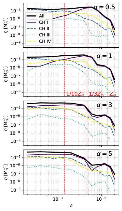
Figure 1: Merger efficiency $\eta$ for BBHs as a function of metallicity $Z$. From top to bottom $\alpha=0.5$, 1, 3, 5. The different colors refer to formation channels I-IV (Section 2.3). The vertical red lines highlight metallicity values of $Z=1/100$, $1/10$, and $1/3$ Z_⊙.

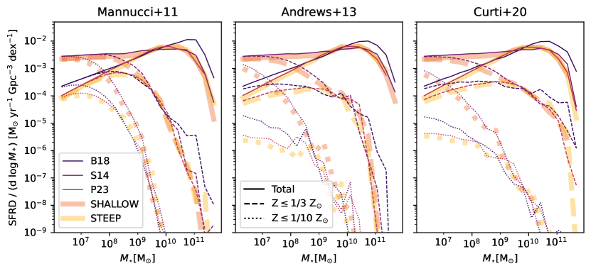
Figure 2: Contribution of galaxies of mass $M_{\ast}$ to the SFR density evaluated for different metallicity thresholds at $z=0$. The x-axis represents the galaxy stellar mass $M_{\ast}$, while the lines show the total contribution to the SFR density from all galaxies in a given stellar mass bin, with a metallicity $Z\leq Z_{\rm th}$. The different line styles refer to different metallicity thresholds $Z_{\rm th}$; solid lines:$Z_{\rm th}=1/3{\rm Z}_{\odot}$, dashed: $Z_{\rm th}=1/10{\rm Z}_{\odot}$ and dotted:$Z_{\rm th}=1/100{\rm Z}_{\odot}$. The different colors represent models with different SFR–$M_{\ast}$ relations, blue: B18, violet: S14, pink: P23, orange: SHALLOW, yellow: STEEP.

The BBH merger efficiency (i.e., the number of BHs that merge per total initial stellar mass) depends on metallicity, being higher for metal-poor stars (Dominik et al., 2012; Giacobbo & Mapelli, 2018; Klencki et al., 2018). With sevn, we find an abrupt drop of three orders of magnitude in the BBH merger efficiency, above $\sim{1/3\,{}Z_{\odot}}$ (Fig. 1). The drop mildly depends on the $\alpha$ parameter: it is close to $1/3$ Z_⊙ for $\alpha\leq 1$ and shifts to lower metallicities ($\sim 1/10$ Z_⊙) for $\alpha=3$ or $5$. For this reason, the fraction of SFR at low metallicity is crucial for determining the BBH merger rate.

3.2 Is the contribution of low-mass galaxies important?

Figure 2 shows the relative contribution of different galaxy masses to the total SFR density and to the SFR density below a certain $Z$ threshold. We consider two reference metallicity thresholds: $Z\leq 1/3\,{}{\rm Z}_{\odot}$ and $\leq{}1/10\,{}{\rm Z}_{\odot}$. We compare the results for different main-sequence definitions. In Figure 2, we emphasize the SHALLOW and STEEP models (wider lines), because they represent the extreme cases: the former has the shallowest trend, whereas the latter has the steepest decrease of the SFR density at low galaxy masses. This Figure shows the results for galaxies at $z=0$; however, the following considerations hold for every considered redshift.

We see from Fig. 2 that only with the shallowest SFR–$M_{\ast}$ relations the contribution from low-mass galaxies is important, for metallicities $Z\leq 1/3$ Z_⊙. For the steepest galaxy main-sequence models (e.g., the STEEP model and P23), most of the SFR for metallicities below $1/3$ Z_⊙ originates from galaxies with masses in the range of $(10^{9}-10^{10})\mathrm{M}_{\odot}$ for the fundamental metallicity relations by Andrews & Martini (2013) and Curti et al. (2020), while the contribution from $10^{6}\mathrm{M}_{\odot}$ galaxies is about half. The peak in SFR shifts towards galaxy masses of $(10^{8}-10^{9})\mathrm{M}_{\odot}$ adopting the models by Mannucci et al. (2011). On the other end, shallower main sequence slopes (e.g. the SHALLOW model, S14) show a similar SFR contribution from low mass galaxies up to $\sim 10^{8}\mathrm{M}_{\odot}$. Model B18 falls in between these two extreme cases.

If we restrict our attention to even lower metallicities ($Z<1/10$ Z_⊙), the contribution from low-mass galaxies becomes important for all the SFR–$M_{\ast}$ relations. As a result, for higher $\alpha$ parameters (for which the merging efficiency peaks at smaller metallicities, see Fig. 1) the contribution from low-mass galaxies becomes important, regardless of the chosen SFR–$M_{\ast}$ relation.

While the trend described above is true for all the fundamental metallicity relations, we see from the different panels that the prescriptions by Curti et al. (2020) and Andrews & Martini (2013) predict on average higher metallicities (Fig. 7).

3.3 Cosmic merger rate density

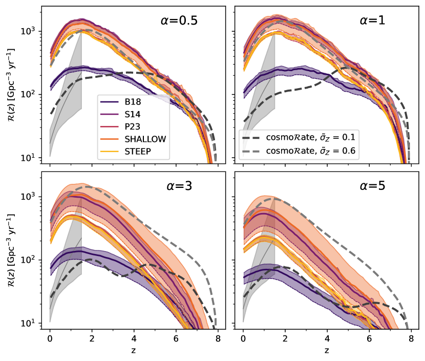
Figure 3: BBH merger rate density as a function of redshift for different observational scaling relations (different colors) and CE $\alpha$ parameters (different panels). Each color is associated with a different SFR–$M_{\ast}$ relation, as summarized in the legend in the top left-hand panel. The solid lines show the model with $M_{\mathrm{min}}=10^{7}$ M_⊙. The shaded area encompasses the difference between $M_{\mathrm{min}}=10^{6}\mathrm{M}_{\odot}$ (upper boundary), and $M_{\mathrm{min}}=10^{8}\mathrm{M}_{\odot}$ (lower boundary). All the models assume the fiducial fundamental metallicity relation by Andrews & Martini (2013). The thick dashed lines show the merger rate density obtained with cosmo$\mathcal{R}$ate (simplified model), assuming the cosmic SFR density by Madau & Dickinson (2014) and a lognormal distribution for the metallicity with a spread $\tilde{\sigma}_{\rm Z}=0.1$ (dark grey) and $0.6$ (light grey). The grey shaded regions show the MRD inferred by the LVK collaboration: $\mathcal{R}(z)\propto(1+z)^{k}$(Abbott et al., 2023b).

Figure 3 shows the BBH cosmic merger rate density we obtain assuming different SFR–$M_{\ast}$ relations, adopting the fundamental metallicity plane by Andrews & Martini (2013). The results for the fundamental metallicity relations by Mannucci et al. (2011) and Curti et al. (2020) are shown in Appendix B. We compare our merger rate densities with the inferred fit $\mathcal{R}(z)\propto(1+z)^{k}$ by the LVK collaboration up to the third observing run (Abbott et al., 2023b).

All predicted BBH merger rate densities exceed the LVK estimates across all our galaxy-derived models. The B18 model yields the lowest merger rate density. This is expected as B18 results in the lowest SFR density (see Figure 6 in Appendix A). This is probably a result of the data sample utilized in B18 reaching up to $z\sim 0.9$. Instead here we are extrapolating the relation to much higher redshifts.

The merger rate densities evaluated by setting different minimum galaxy masses differ at most by a factor of $\sim 2$. Even removing all the galaxies with mass below $10^{8}\mathrm{M}_{\odot}$, the merger rate density is still well above the 90% credible interval from LVK. The magnitude of the difference between assuming $M_{\rm min}=10^{6}$, $10^{7}$ and $10^{8}\mathrm{M}_{\odot}$ depends on the main sequence definition adopted. As expected, steeper SFR–$M_{\ast}$ relations result in smaller differences with the minimum galaxy stellar mass adopted.

The differences between $M_{\rm min}=10^{6}$, $10^{7}$, and $10^{8}\,{}\mathrm{M}_{\odot}$ are bigger for $\alpha=3$ and $\alpha=5$, compared to $\alpha=1$ or $\alpha=0.5$, as expected from the results described in Section 3.2).

Figure 4 also compares the merger rate density we obtain through our host-galaxy models (i.e., with galaxy$\mathcal{R}$ate) with the merger-rate density calculated adopting an average SFR density and metallicity evolution of the Universe (i.e., with cosmo$\mathcal{R}$ate). The merger rate density we obtain modelling the host galaxies with observational scaling relations and the one we estimate by assuming an average SFR density agree only when we assume a large metallicity spread ($\tilde{\sigma}_{\rm Z}=0.6$, see Sec. 2.4) for the latter.

Moreover, even assuming a large value of $\tilde{\sigma}_{\rm Z}$, the predicted shape and steepness of the merger rate density differ in the two models, especially at high redshift and for models with $\alpha>1$.

3.4 Formation channels

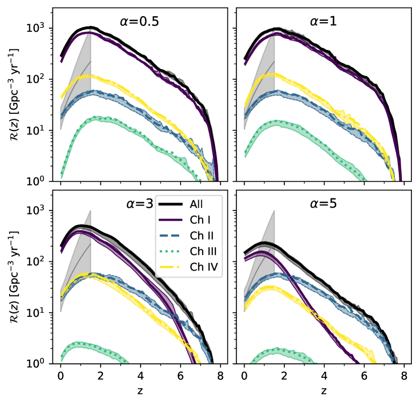
Figure 4: BBH merger rate density as a function of redshift for different BBH formation channels. The solid black lines show the merger rate density of the whole BBH population. The shaded area encompasses the difference between $M_{\mathrm{min}}=10^{6}\mathrm{M}_{\odot}$ (upper boundary), and $M_{\mathrm{min}}=10^{8}\mathrm{M}_{\odot}$ (lower boundary). The different panels show the results obtained assuming different CE $\alpha$ parameters. All the models assume the fiducial SFR–$M_{*}$ relation P23 and the fundamental metallicity relation by Andrews & Martini (2013). The grey shaded regions show the MRD inferred by the LVK collaboration (Abbott et al., 2023b).

Figure 4 shows the merger rate density for each BBH formation channel, as defined in 2.3, through equation 12. Channel I (traditional CE scenario, with at least one CE phase after the formation of the first BH) gives the main contribution to the full BBH merger rate density at all redshifts, if $\alpha\leq 1$. Channel I is subdominant only at high redshift and when $\alpha>1$. This is the result of longer delay time distributions for channel I, compared to channels II and IV. As a consequence, even if the merger efficiency of channel I is higher at all metallicities (Figure 1), channels II and IV dominate the merger rate density at high redshift. Moreover, the longer delay times result in a much steeper shape of the merger rate density for channel I, especially if we adopt a large value of $\alpha$.

At low redshift, the merger-rate density associated with channel I is always largely above the LVK 90% credible interval. In contrast, the merger rate densities associated with channels II (stable mass transfer), III and IV lie within the observed range reported by LVK for all the considered $\alpha$ parameters. Channel III is by far the least common formation pathway.

4 Discussion

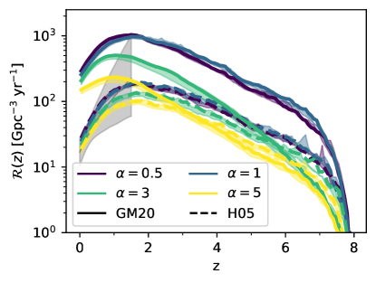
Figure 5: Merger rate density as a function of redshift, for the natal-kick models GM20 (solid lines) and H05 (dashed lines). The line colors show the results obtained assuming different CE efficiency parameters ($\alpha$). The upper boundaries of the shaded areas show the models obtained with minimum galaxy mass $M_{\ast}=10^{6}\mathrm{M}_{\odot}$, whereas for the lower boundary the minimum mass is $10^{8}\mathrm{M}_{\odot}$. All the models assume the fiducial observational scaling relations. The grey shaded region shows the MRD inferred by the LVK collaboration (Abbott et al., 2023b).

In this work, we have modeled the host galaxies of BBHs, their SFR and metallicity with the most up-to-date observational scaling relations. Nevertheless, as we improve the description of the metal-dependent SFR, the BBH merger rate density we obtain at low redshift ($10^{2}-10^{3}\,{}\mathrm{Gpc}^{-3}\mathrm{yr}^{-1}$) is always well above the 90% credible interval inferred by LVK after the third observing run (Fig. 3). This is true for all of our models, considering different SFR–$M_{\ast}$ relations, different fundamental metallicity relations, and different values of the efficiency parameter for CE ejection.

Our results are consistent with the merger rate densities recently calculated by Boesky et al. (2024a), adopting the compas binary population synthesis code (COMPAS et al., 2022). So, we exclude that the overestimate of the BBH merger rate density is a feature of our population-synthesis code sevn (Iorio et al., 2023). Rather, it is a problem common to current population synthesis codes.

In the following, we discuss several potential solutions to reconcile theoretical predictions and GW data. One possible explanation is that the CE phase occurs less frequently than previously assumed, or that BBH progenitors do not survive the CE phase as often as currently believed. Conversely, the stable mass transfer (channel II) may play a considerably more significant role in BBH formation than previously expected, as already proposed by several authors (Neijssel et al., 2019; Klencki et al., 2020, 2021; Bavera et al., 2021; Marchant et al., 2021). In binary population synthesis codes, the CE channel tends to dominate over the others; in contrast, stable mass transfer is prevalent in detailed stellar-structure calculations Gallegos-Garcia et al. (2021). One of the main factors of uncertainty lies in the criteria for the onset of a CE phase. As proposed by Ge et al. (2020), mass transfer might be stable for a wider range of mass ratios than previously believed, at least under the assumption of adiabatic, conservative mass transfer. Another slightly different interpretation is that the traditional description of semi-major axis evolution during a CE phase (based on the $\alpha$ parameter, Hurley et al. 2002) is too simplified, and does not capture the actual evolution of the system (Hirai & Mandel, 2022; Trani et al., 2022; Di Stefano et al., 2023; Everson et al., 2024). If the orbital separation during a CE phase shrinks less than predicted by the traditional $\alpha$ formalism, then the resulting merger rate density is likely going to be lower (e.g. Renzo et al., 2023).

Natal kicks also significantly influence the merger rate density (Mapelli & Giacobbo, 2018; Iorio et al., 2023; Boesky et al., 2024a). In Fig. 5, we compare our fiducial model with a model in which natal kicks are drawn from a Maxwellian distribution with root-mean square velocity $\sigma=265$ km s^-1, without accounting for the fallback (Hobbs et al., 2005). This model yields substantially higher kicks, leading to lower BBH merger rate densities across all considered $\alpha$ parameters. Thus, another possible way to reconcile observed and predicted merger-rate density is to assume that natal kicks are higher than usually expected for BBHs. However, this also has an impact on the BH mass function, favouring the merger of more massive binary systems (Iorio et al., 2023).

Finally, recent work by Schneider et al. (2021) shows that envelope stripping can affect the final fate and compact remnant mass of massive stars, increasing the minimum zero-age main sequence mass of BH progenitors from $\sim 30$ M_⊙ to $\sim 70\mathrm{M}_{\odot}$. While population calculations still need to be done for this scenario, this might result in a decrease of the BBH merger rate density as well.

A few caveats should be added. Recent work by Rinaldi et al. (2022) suggests that starburst galaxies contribute to 60$-$90% of the total SFR. Rinaldi et al. (2022) find a clear bimodality between the galaxy main sequence and the starburst sequence for higher massive galaxies, $M_{\ast}\geq 10^{9}\mathrm{M}_{\odot}$. Our current approach likely underestimates the impact of starburst galaxies (see also Caputi et al., 2017; Bisigello et al., 2018). Improved modelling of starburst galaxies is beyond the scope of this work. Nevertheless, an higher contribution of starburst galaxies would further increase the predicted BBH merger rates as they tend to be more metal-poor than main sequence galaxies. We would like to remark that models based on the evolution of the average SFR and metallicity over cosmic time (Santoliquido et al., 2021, e.g.) broadly capture the BBHs merger rate densities (Fig. 3)., when accounting for a wide spread in metallicity for a given redshift bin ($\tilde{\sigma}_{\rm Z}=0.6$). This assumption is needed to mimic the complex distribution of metallicities that in our detailed approach naturally results from the spread in galaxy masses and SFRs.

Finally, in our work, we are completely neglecting the dynamical formation of BBHs in star clusters and galactic nuclei. However, including this channel would only lead to a further increase of the merger rate density because dynamics is known to boost the merger rate density even in a metal-rich environment (Rodriguez & Loeb, 2018; Di Carlo et al., 2020; Mapelli et al., 2022; Barber & Antonini, 2024).

5 Summary

We have studied the merger rate density of BBHs across cosmic time over an extensive grid of parameters, exploring the effects of different galaxy observational scaling relations and binary evolution models. Furthermore, we have studied the relative impact of different isolated BBH formation channels on the merger rate density. We can summarize our main results as follows.

• Current models of binary population synthesis predict values of the BBH merger rate density at redshift $z\leq{1}$ that are well above the 90% credible interval inferred from LVK data (Abbott et al., 2023b). Differences between the BBH mass function obtained from population-synthesis calculations and the one assumed to infer the LVK rates, might bias the comparison between the two merger rate densities. However, the discrepancy between predictions and LVK rates (at least a factor of $\sim{10}$) is too large to be fully accounted for by such BBH mass function differences.

• The impact of low-mass galaxies ($M_{\ast}<10^{8}$ M_⊙) on the BBH merger rate density is highly dependent on the steepness of the SFR–$M_{\ast}$ relation. For steep SFR–$M_{\ast}$ relations (P23), galaxies with mass $M_{\ast}\lesssim 10^{7}\mathrm{M}_{\odot}$ do not contribute significantly to the merger rate density.

• Even removing all the galaxies with mass below $10^{8}$ M_⊙ (hence, with lower metallicity), the merger rate density is still well above the 90% credible interval from LVK. Thus, uncertainties in the number of low-mass galaxies do not dramatically affect the merger rate density and do not solve the tension between predicted and observed BBH merger rate density.

• Models based on the average SFR and metallicity evolution need to account for the whole metallicity spread at a given redshift $\tilde{\sigma}_{\rm Z}\sim 0.6$ in order to mirror detailed Universe prescriptions. In this case, the merger rate densities predicted by the two approaches broadly agree, with differences that become more noticeable towards high redshifts.

• The merger rate density of BBHs is dominated by Channel I, where the systems evolve through at least one CE phase only after the first compact object formation.

Overall, our results clearly indicate that there is a tension between current models of BBH merger rates and values inferred from GW data. We cannot explain this tension through uncertainties on the cosmic SFR density, as we have adopted state-of-the-art models, robustly grounded in observations. Future studies are requested to understand the origin of this tension, addressing -e.g.,- the nature of core collapse, the stability of mass transfer, and the magnitude of natal kicks.

Appendix A Observational scaling relations

Below, we provide the details of the observational scaling relations adopted in this work. We follow the approach presented by Santoliquido et al. (2022).

A.1 Galaxy stellar mass function

Our adopted galaxy stellar mass function takes the form of a Schechter function:

$$\phi(M_{\ast},z)\,{}dM_{\ast}=\phi_{\rm N}(z)\,{}e^{-M_{\ast}/M_{\rm cut}(z)}\left(\frac{M_{\ast}}{M_{\rm cut}(z)}\right)^{-\alpha_{\rm GSMF}}dM_{\ast},$$ (14)

where $\phi_{\rm N}(z)$ is a normalization factor and $M_{\rm cut}(z)$ is the galaxy stellar mass at which the function transitions from a power law at low masses to an exponential decay at high masses. In our models, we use the fit derived by Chruslinska & Nelemans (2019) and based on a wide catalog of galaxy stellar mass function relations over separate redshift bins.

A.2 Star formation rate (SFR)

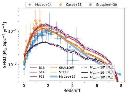
Figure 6: SFR density as a function of redshift for different SFR-$M_{\ast}$ relations (different colors). The different linestyles show the results by cutting the galaxy main sequence at different minimum galaxy masses, $M_{\rm min}=10^{6}\mathrm{M}_{\odot}$ (dotted), $10^{7}\mathrm{M}_{\odot}$ (solid) and $10^{8}\mathrm{M}_{\odot}$ (dashed). The wide blue line shows the fit by Madau & Fragos (2017). The markers show observed data points: the blue dots are are taken from Madau & Dickinson (2014), the orange diamonds are from Casey et al. (2018), and the purple squares are taken from Gruppioni et al. (2020).

We draw the SFR of galaxies from the following double lognormal distribution (Sargent et al. 2012; Rodighiero et al. 2015; Schreiber, C. et al. 2015):

$$\mathcal{P}(\log{\rm SFR}|M_{\ast},z)=A_{\rm MS}\exp\left[-\frac{\left(\log{\rm SFR}-\langle\log{\rm SFR}\rangle_{\rm MS}\right)^{2}}{2\sigma_{\rm MS}^{2}}\right]+\\ A_{rmSB}\exp\left[-\frac{\left(\log{\rm SFR}-\langle\log{\rm SFR}\rangle_{\rm SB}\right)^{2}}{2\sigma_{\rm SB}^{2}}\right],$$ (15)

where $A_{\rm MS}=0.97$ and $A_{\rm SB}=0.243$ constants (Sargent et al. 2012). $\langle\log{\rm SFR}\rangle_{\rm MS}$ and $\sigma_{\rm MS}$ are the average SFR of the main sequence and its dispersion. We adopt several definitions of the galaxy main sequence, as described in section 2.4. For all of our models we use the fiducial value $\sigma_{\rm MS}=0.188$ dex (Santoliquido et al. 2022). In a similar way, $\langle\log{\rm SFR}\rangle_{\rm SB}$ and $\sigma_{\rm SB}$ are the average and the standard deviation of the galaxy starburst sequence. The latter is defined as in Sargent et al. (2012),

$$\langle\log{\rm SFR}\rangle_{\rm SB}=\langle\log{\rm SFR}\rangle_{\rm MS}+0.59$$ (16)

Moreover, we assume $\sigma_{SB}=0.243$ dex.

We couple the galaxy stellar mass function with the distribution of SFR as described above. By integrating the SFR for each redshift bin, we get the SFR density as a function of redshift, shown in Fig. 6. We compare the predicted SFR density for all the adopted galaxy models. All the galaxy main sequence models predict SFR densities which are consistent with the data from Madau & Dickinson (2014). Moreover, varying the lower mass limit of the galaxy main sequence (represented by different line styles) does not significantly impact the SFR density.

A.3 Fundamental metallicity relations

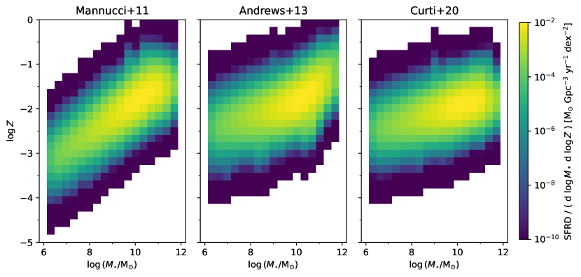
Figure 7: SFR density per galaxy mass (x-axes) and metallicity bins (y-axes) at $z=0$. Each panel shows the result for a different FMR relation, from left to right: Mannucci et al. (2011), Andrews & Martini (2013) and Curti et al. (2020).

We consider three different fundamental metallicity relations. We adopt the fit from Mannucci et al. (2011):

$$\begin{split}12+\log\left(\mathrm{O/H}\right)&=8.90+0.37m-0.14s-0.19m^{2}\\ &+0.12ms-0.054s^{2}\quad\;\mathrm{for}\;\mu_{0.32}\geq 9.5\\ &=8.93+0.51(\mu_{0.32}-10)\quad\;\mathrm{for}\;\mu_{0.32}<9.5\end{split}$$ (17)

where $m=\log M_{\ast}-10$ and $s=\log{\rm SFR}$ and $\mu_{0.32}=\log M_{\ast}-0.32\log{\rm SFR}$, all the quantities are in solar units.

We derive an additional fit for the fundamental metallicity relation based on figure 12 by Andrews & Martini (2013)

$$12+\log\left(\mathrm{O/H}\right)=0.43(\log M_{\ast}-0.66\log{\rm SFR})+4.59$$ (18)

Lastly, we consider the metallicity relation calculated in Curti et al. (2020):

$$12+\log\left(\mathrm{O/H}\right)=Z_{0}-\gamma/\beta\log\left(1+(M_{\ast}/M_{0}(\mathrm{SFR}))^{-\beta}\right)$$ (19)

where $M_{0}(\mathrm{SFR})=m_{0}+m_{1}\log{\rm SFR}$ and $Z_{0}=8.779\pm 0.005$, $m_{0}=10.11\pm 0.03$, $m_{1}=0.56\pm 0.01$, $\gamma=0.31\pm 0.01$ and $\beta=2.1\pm 0.4$.

For the purposes of our simulations, we convert these relations into absolute metallicities. We adopt the solar metallicity values from Caffau et al. (2011): $Z_{\odot}=0.0153$ and $12+\log(\mathrm{O/H})_{\odot}=8.76$.

Figure 7 compares the distributions of SFR density as a function of galaxy stellar mass and metallicity, for different fundamental metallicity relations at $z=0$. The differences are particularly noticeable for low–mass galaxies, where the model by Mannucci et al. (2011) clearly predicts lower metallicities compared to the other two prescriptions. Curti et al. (2020) predicts the flattest relation, with less than an order of magnitude difference in metallicty between the low and high–mass galaxies.

Appendix B Merger rate densities

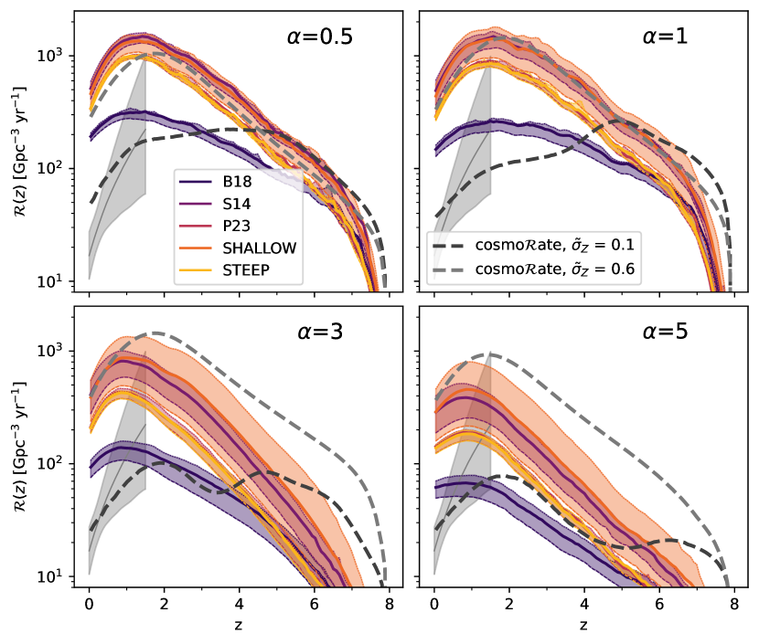
Figure 8: Same as Fig. 3 but for the fundamental metallicity relation by Curti et al. (2020).

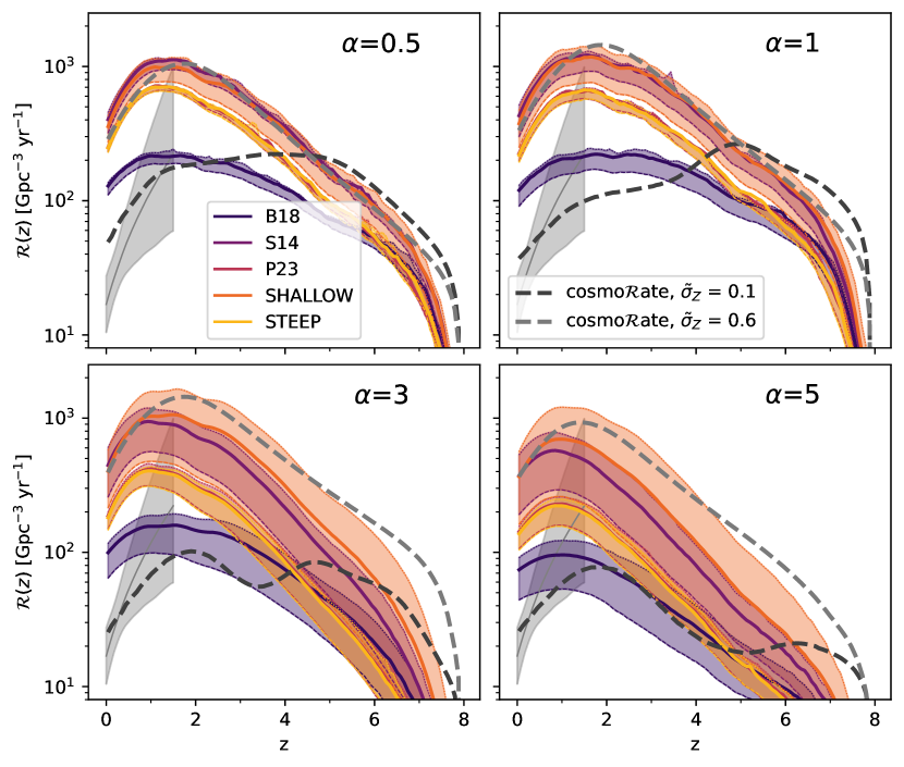
Figure 9: Same as Fig. 3 but for the fundamental metallicity relation by Mannucci et al. (2011).

Figures 8 and 9 show the BBH cosmic merger rate densities obtained for different SFR–$M_{*}$ relations, adopting the fundamental metallicity relations by Curti et al. (2020) and Mannucci et al. (2011), respectively.