*\pagemark
Sufficient Condition on Bipartite Consensus of Weakly Connected Matrix-weighted Networks
Abstract
Recent advances in bipartite consensus on matrix-weighted networks, where agents are divided into two disjoint sets with those in the same set agreeing on a certain value and those in different sets converging to opposite values, have highlighted its potential applications across various fields. Traditional approaches often depend on the existence of a positive-negative spanning tree in matrix-weighted networks to achieve bipartite consensus, which greatly restricts the use of these approaches in engineering applications. This study relaxes that assumption by allowing weak connectivity within the network, where paths can be weighted by semidefinite matrices. By analyzing the algebraic constraints imposed by positive-negative trees and semidefinite paths, we derive new sufficient conditions for achieving bipartite consensus. Our findings are validated by numerical simulations.
Index Terms:
Consensus, Bipartite consensus, Weak Connectivity1 Introduction
Achieving collective behaviors among a group of identical agents has been a prominent research topic across various domains, including social networks [1, 2], coupled oscillator systems in power grids [3], and the control of groups of robots such as unmanned ground vehicles [4], unmanned aerial vehicles [5], and unmanned underwater vehicles [6]. In addition to the dynamics of each agent, communication protocols play a crucial role in facilitating these collective group behaviors [7, 8, 9]. Early scalar-weighted protocols commonly used a scalar quantity for each pair of communicating agents. While this approach ensures consensus among high-dimensional agents with minimal requirements on network topology, it does not fully utilize the extra communication capacity of the agents. In contrast, recent research extends this concept by using a matrix—typically non-diagonal—for each pair of agents [10, 11, 12], which reduces to the scalar-weighted case when each matrix is a scalar multiple of the identity matrix. A network employing this matrix-based protocol is called the matrix-weighted network. It is shown to capture more complex, inter-dimensional interactions and lead to more intricate group behaviors [10, 13, 14, 15].
Among these group behaviors, bipartite consensus represents a specific distribution of the agents. When reaching bipartite consensus, agents are divided into two groups based on their states: one group consists of agents with identical steady-state behaviors, while the other group comprises agents with opposing steady-state behaviors. Bipartite consensus finds applications in various fields, including social networks [2], coupled oscillator systems [16], and multi-robot systems [17, 18]. This concept is also crucial for understanding the more general case of cluster consensus, as bipartite consensus represents a special instance of cluster consensus involving two clusters.
Research has focused on the conditions under which a matrix-weighted network can achieve bipartite consensus. Given that the matrix-weighted network can be modeled as a linear time-invariant system characterized by a matrix-valued graph Laplacian , the asymptotic behavior of bipartite consensus is influenced by the structure of the null space of the system matrix, . In [19], a necessary and sufficient condition for achieving bipartite consensus was provided, based on the algebraic properties of . In contrast, [20] proposed a necessary condition from the perspective of network structure. This condition involves the concept of a nontrivial balancing set, which, among other things, divides the agents into two groups that are negatively interacting, i.e., having negative connections in between. The study [20] further shows that for a network to reach bipartite consensus, the communication graph must contain a unique nontrivial balancing set among all possible divisions. Although these conditions are theoretically elegant, they lack practical design guidelines, such as sufficient conditions that engineering practitioners can use to design matrix weights and network structures to achieve bipartite consensus without being overly conservative. In [11] and [12], sufficient conditions are presented that require the communication graph to have either a positive or a positive-negative spanning tree. We refer to matrix-weighted networks with such a spanning tree as a strongly connected network.
These requirements however, are not always met in practical applications. For example, [14] applied the matrix-weighted protocol in a sensor network where the connections are weighted solely by semidefinite matrices. This network, lacking a positive-negative spanning tree, is referred to as a weakly-connected matrix-weighted network. Similar cases appear in coupled oscillator systems [10, 21] and opinion dynamics [22]. This motivates this work, which aims to provide sufficient conditions to ensure bipartite consensus on weakly-connected matrix-weighted networks.
The weakly-connected matrix-weighted network poses a unique challenge on the analysis of the Laplacian null space. The block Laplacian matrix defined on these networks exhibits complex spectral properties and null space behavior that are not characterized by traditional graph metrics. To address this, we introduce new connectivity concepts to partition the graph into components – the strongly connected subgraphs spanned by positive-negative trees and the semidefinite paths between them – enabling a more targeted null space analysis. By exploring various necessary or sufficient conditions, we develop a theorem that establishes the relationship between the Laplacian null space and the network’s structural and weight configurations, which further ensures bipartite consensus. This work provides a theoretical framework that not only addresses the bipartite consensus phenomenon but also offers broader insights for designing and analyzing matrix-weighted networks.
The paper is organized as follows. Section 2 introduces notations and preliminary results of matrix-weighted networks. Section 3 presents the definition and properties of the continent, followed by the main theorem on achieving bipartite consensus. Numerical examples are demonstrated in Section 4 to validate our theorem. Section 5 gives concluding remarks.
2 Preliminaries and Problem Formulation
This section covers the necessary preliminaries, including notations, graph theory, problem formulation, and the relevant propositions.
2-A Notations
Let , and be the set of real numbers, natural numbers and positive integers, respectively. For , we denote . For , the symbol denotes its Euclidean norm. For a set , denotes its cardinality. For a symmetric matrix , we express its positive (negative) definiteness with (), and its positive (negative) semidefiniteness with (). In addition, a matrix-valued sign function is defined such that
The notation is adopted for to denote .
For a matrix , denotes the column space of , which is the linear span of its column vectors. Given a set of vectors , we define the matrix that stacks these vectors, assuming the vectors are well ordered. For a matrix with , let represent the set of its eigenvectors corresponding to the eigenvalue zero. This gives along with . The notation represents a diagonal matrix whose diagonal elements are taken from the sequence in . Meanwhile, denotes a block diagonal matrix whose off-diagonal blocks are zero matrices, and the matrices in form the diagonal blocks. For subsets of , the Minkowski sum is expressed as . Additionally, we define the set for .
2-B Graph Theory
(Graph) Define the matrix-weighted graph/network as a triplet , where has order . The simple graph, which is the scope of this work, is a graph where the connections are undirected and are without self-loop or multiple edges. A node in is also referred to as an agent , where is a bijection on and will be written as . An edge is then the pair . The function maps the edge to its associated weight matrix, i.e., .
(Laplacian) In this paper, the weight matrices are considered to be real symmetric, which furthermore have or if , and otherwise, for all . When we refer to the edge as a semidefinite edge, while to with , a definite edge. The adjacency matrix for a matrix-weighted graph is then a block matrix such that the block on the -th row and the -th column is . Let be the neighbor set of an agent . We use to represent the matrix-weighted degree matrix of a graph where . The matrix-valued Laplacian matrix of a matrix-weighted graph is defined as , which is real symmetric. A gauge matrix in this paper is defined by the diagonal block matrix , where ,
(Path) On a matrix-weighted graph , a path is defined as a sequence of edges as where are all distinct and are called endpoints. Two paths are node-independent if the nodes they traverse have none in common. The sign of a path is defined as . The null space of the path is defined as , where is the Minkowski sum. We say is a definite path if , and is a semidefinite path if and .
(Tree. Cycle.) A positive-negative tree on a matrix-weighted graph is a tree such that , it satisfies that . A positive-negative spanning tree of is a positive-negative tree traversing all nodes in . A cycle of is a path that has the same node as endpoints, i.e., .
Definition 2.1 (Weakly Connected).
A matrix-weighted network is called weakly connected if does not have a positive-negative spanning tree.
Definition 2.2 (Structural Balance).
A matrix-weighted network is structurally balanced if there exists a bipartition of nodes , such that the matrix-valued weight between any two nodes within each subset is positive (semi-)definite, but negative (semi-)definite for edges connecting nodes of different subsets. A matrix-weighted network is structurally imbalanced if it is not structurally balanced.
Definition 2.3 (Nontrivial Balancing Set).
Let be a matrix-weighted network and be a partition of . A Nontrivial Balancing Set (NBS) defines a set of edges of such that, (I) the negation of the signs of their weight matrices renders a –structurally balanced graph, and (II) the null spaces of their weight matrices have intersection other than , which is denoted as .
Remark 2.4.
When because is itself –structurally balanced, we define in this case suppose . An NBS is unique in if for any other partition of , such set of edges does not exist.
2-C Problem Statement
Consider a multi-agent network of agents. The states of each agent is denoted by where . The interaction protocol for the matrix-weighted network reads
| (1) |
where denotes the weight matrix on edge . The collective dynamics of the multi-agent network (1) can be characterized by
| (2) |
where and is the matrix-valued graph Laplacian. The control objective for the system (1) is related to the following definition.
Definition 2.5 (Bipartite Consensus).
The system (1) achieves bipartite consensus if there exist a partition and , such that, for all initial values other than there is and , .
The control objective is to determine the configuration of the network (1), in terms of its structure and weight matrices, that is sufficient to guarantee an asymptotic bipartite consensus solution, given that the network is weakly connected.
2-D Network Properties
The following results establish fundamental properties of network (1) that are essential for proving our main results.
Lemma 2.6.
For matrix-weighted network in (1) whose Laplacian has , where are the orthonormal eigenvectors, exists and .
Proof:
According to [20, Lemma 1], the matrix-valued Laplacian satisfies
where is the signed incidence matrix; since is positive semi-definite, there is . The fact that the Laplacian matrix is real and positive semidefinite guarantees that it is diagonalizable, implying all Jordan blocks for eigenvalue zero having dimension one. This ensures the system’s convergence to the equilibrium that satisfies . As for the value of , consider the system response where is the orthogonal matrix that satisfies , . Therefore we have , and . ∎
Proposition 2.7.
Remark 2.8.
The following proposition demonstrates that the bipartite consensus solution corresponds to a specific structure of the Laplacian null space.
Proposition 2.9.
In [20], another interpretation of bipartite consensus on the matrix-weighted network is provided from the graph-theoretic perspective instead of the purely algebraic, which relies on the concept of the Nontrivial Balancing Set (see Definition 2.3). For now, we denote where the columns of the matrix span the space of dimension . We see that the uniqueness of the NBS constitutes a first necessary condition of the bipartite consensus achieved on (1) with general topology.
Proposition 2.10.
Proposition 2.11.
Proposition 2.12.
Unless otherwise specified, the matrix-weighted networks studied in this work are meant to be connected. As we point out in the following Lemma, this assumption is de facto necessary for bipartite consensus.
Lemma 2.13.
Proof:
Assume that bipartite consensus is achieved in the sense of Definition 2.5 on network (1) that is unconnected between and , . Then there exists a nontrivial balancing set in the network such that, by changing the signs of the matrix weights of the edges in , the network is rendered structurally balanced; since structural balance is a global property, the subgraphs based on and that are independent of each other are also rendered structurally balanced. This suggests that the subgraphs , both have their own nontrivial balancing sets, and according to Proposition 2.10, , , where are the Laplacians of , , while the Laplacian of can be arranged as
Thus we know
for and bipartite consensus of the entire system is not achieved in the sense of Definition 2.5. Therefore the assumption does not stand, and bipartite consensus must be achieved with the precondition that the network is connected. ∎
3 Main Results
This section provides sufficient conditions for the agents to achieve bipartite consensus on a weakly connected network (1). Generally, a matrix-weighted network can be divided into the strongly connected parts – subgraphs spanned by positive-negative trees – and the weak, semidefinite, connections between them. This section introduces the concept of a “continent” for the strongly connected part. It is then discussed how the network can achieve bipartite consensus when several “continents” are linked by weak connections known as the semidefinite paths.
3-A Continents
This subsection defines a strongly connected component of a matrix-weighted graph, called a continent, and discusses its structural and dynamic properties related to the NBS.
Definition 3.1 (Continent).
Given a matrix-weighted network whose matrices are of dimension , a maximal positive-negative tree is a positive-negative tree such that , there does not exist a definite path with and as endpoints. A continent of is then the subgraph where , , and .
Since a continent is essentially a subgraph of , the concept of NBS is directly applied to . Here we discuss the properties of a continent as only part of a matrix-weighted graph in the presence of a unique NBS.
Lemma 3.2 states that structurally, a continent must have a unique NBS if the entire graph has a unique NBS, and that the two NBSs have identical partitions for the agents of the continent.
Lemma 3.2.
Assume that is a connected matrix-weighted network with a unique NBS , and is a continent of , then also has a unique NBS . Moreover, the bipartitions and are identical for all .
Proof:
Since an NBS for exists, that is, after the negation of the signs of every , becomes structurally balanced, then any subgraph of can also turn structurally balanced by negating in a subset of , where the edges have weights with nontrivially intersecting null spaces. Thus an NBS for a subgraph of exists, and there is an NBS for . By definition, the continent has a maximal positive-negative tree . We will show that is unique on , and the bipartition conforms that given by .
The bipartition of given by is defined as such: , if the path on between and is positive, then ; otherwise, . Since any weight matrix of is positive or negative definite and exists, must include edges other than those of to have , thus the bipartition of is undisturbed, and . On the other hand, if there exists that yields any other bipartition, at least one edge of must be selected into for negation, then there will be the contradiction . For the same reason, the bipartition made for conforms that of . ∎
Corollary 3.3.
For a matrix-weighted network with a unique nontrivial balancing set and continents , if an edge , then . In addition, there is
Dynamically, the steady-states of the agents of the continent can also be characterized by its NBS, which involves the NBS’s nontrivially intersecting null space. Let us first introduce a basis representation of some NBS-related null spaces that will come in handy for the mathematical statements.
Definition 3.4 (Basis for Null Space).
For a matrix-weighted network , if there exists an NBS with a nontrivially intersecting null space , denote the basis of this null space as set , which corresponds to a matrix whose columns are the basis vectors. Suppose are continents of . For , if an NBS of the subgraph exists, denote it as whose nontrivially intersecting null space is . Similarly, denote the basis of as set , whose corresponding matrix is .
Combining Proposition 2.12 and Lemma 3.2, we derive the following lemma about the steady-states of the agents on the continent.
Lemma 3.5.
Assume that is a connected matrix-weighted network with a unique NBS , and is a continent of , then the Laplacian matrix of the subgraph satisfies , where is a gauge matrix. Therefore, within the entire system (1), the agents of the continent achieve bipartite consensus in the sense of Definition 2.5 and the asymptotic value of agent satisfies .
Proof:
Proposition 2.12 states that, a matrix-weighted network with a positive-negative spanning tree admits bipartite consensus if and only if there is a unique NBS in the graph, while to admit the bipartite consensus solution is to have the null space of its Laplacian as the bipartite consensus subspace (Proposition 2.9). By Lemma 3.2, continent has along with a unique NBS , thus as a subgraph meets where is a gauge matrix. This means that under the constraints imposed by , the agents of converge as . As we evaluate the whole system , what remains unchanged is the bipartite solution obtained by solving eqn.(3) along . Meanwhile, as we solve eqn.(3) on , additional constraints are put on thus its solution space may reduce from ; nevertheless, the bipartition for remains because of , and the statement stands. ∎
3-B Continents Connected with Semidefinite Paths
Now the semidefinite paths connecting the continents are considered to determine the steady-state solution of the entire system. Without loss of generality, the semidefinite paths discussed here do not contain nodes from the continents, apart from their endpoints. Suppose the matrix-weighted network (1) has continents . It can be shown that for any pair of continents connected with semidefinite paths , the asymptotic values of agents satisfy the following equations:
| (4) |
According to Lemma 3.5, represents the convergence value of all agents in , provided there is a unique NBS. Therefore, the solution to eqn. (4) determines whether agents of continents achieve bipartite consensus, leading to the following sufficient condition in Lemma 3.6 to ensure bipartite convergence between different continents.
Lemma 3.6.
Assume that a matrix-weighted network (1) with a unique NBS has continents . Then the agents of the continents achieve bipartite consensus if, for any connected with semidefinite paths ,
| (5) |
hold for or .
Proof:
According to Lemma 3.5, since the network (1) has a unique NBS, agents of the same continent achieve bipartite consensus, that is, , there is . Let , , where , , and . Then in light of Proposition 2.7, by cancelling out along all the semidefinite paths between and , we show that , are subject to constraints
This in turn means that and are subject to constraints (I) and (II) for any . It is then straightforward that all the agents of continents achieve bipartite consensus if for any exactly one set of equations between and have a trivial solution, yielding or , .
Remark 3.7.
Lemma 3.6 implies that exactly one set of equations between (I) and (II) has a trivial solution in order to achieve bipartite consensus.
With the help of Lemma 3.6, the main result of this paper is captured in Theorem 3.8, with its proof in Appendix.
Assumption 1: The matrix-weighted network has a unique NBS .
Theorem 3.8.
For a matrix-weighted network with continents , assume Assumption 1 holds. If, for any , meets the following conditions:
(1) any semidefinite path between two arbitrary continents and satisfies equation (5).
(2) any two semidefinite paths connecting continents and , excluding their endpoints, are node-independent;
(3) for any semidefinite path connecting continents and , its weight matrices have linearly independent bases of null spaces, i.e., the columns of are linearly independent;
(4) for a semidefinite path connecting continents and with , the bases , and the basis of are linearly independent;
then under protocol (1) all the agents of achieve bipartite consensus for almost all initial values.
Theorem 3.8 provides sufficient conditions to achieve bipartite consensus in the presence of a weakly connected graph. While these conditions are straightforward for engineering practitioners to verify, it is important to emphasize that they are not overly conservative.
As shown in Proposition 2.11, Assumption 1 is a necessary condition for achieving bipartite consensus. Once it is satisfied, Conditions (1)–(4) are sufficient to guarantee bipartite consensus, though none of them is sufficient individually. Within the four conditions, (2) plays a central role by imposing a specific constraint on the network structure.
While Condition (1) provides sufficient condition that applies to agents of the continents, it is easy to find examples where the violation of (1) leads to steady-state distribution that is not bipartite consensus (see Section 4). When Assumption 1 and Conditions (1) and (2) hold, Conditions (3) and (4) become both necessary and sufficient to achieve bipartite consensus, thus do not further compromise the generality of the theorem (see Claim .1). This demonstrates that the conditions presented in Theorem 3.8 strike a balance between necessity and practicality.
We now explain Condition (2) in more detail. Condition (2) requires that any two semidefinite paths connecting two continents of the network do not share any intermediate nodes. For instance, in Figure 1, three semidefinite paths connect the two continents: . Although paths and have common endpoints (1 and 4), Condition (2) requires that their intermediate nodes do not overlap, i.e. . However, if there exists an additional semidefinite edge , then the path would share node 9 with path , thereby violating Condition (2).
Although Condition (2) narrows the focus to ensure sufficiency, it is worth noting that alternative sufficient conditions can be derived based on it to achieve bipartite consensus. For instance, when two semidefinite paths share certain agents, provided these paths either have no edge in the NBS (as described by eqn. (7)) or only one edge in the NBS (as described by eqn. (9)), our analysis remains valid. Under this new condition, bipartite consensus can still be guaranteed when combined with Assumption 1 and Conditions (1), (3) and (4). This further demonstrates that the conditions presented in Theorem 3.8 are not overly conservative.
4 Simulation Example
Numerical examples are presented in this section to validate Theorem 3.8 and compare it with existing results.
Example 4.1.
Network in Figure 1 consists of two continents, of agents , of agents , and three connecting semidefinite paths that are . The weight matrices are determined with the following positive definite matrix and positive semidefinite matrices , where
We adopt () for the positive(negative) definite matrices in network , and assign , , , , , , .
We now check for each condition in Theorem 3.8.
Assumption 1 The network is structurally imbalanced due to the four negative cycles in the graph. It is then observed that there exists a unique NBS with , whose negation of signs turns the graph structurally balanced between .
Condition (1) The two continents each has a semidefinite edge or that constitutes its NBS, thus . Take the asymptotic values and as the representatives of and , we find the constraints of semidefinite paths and to be characterized by equation (I) in Lemma 3.6, and , equation (II). As , , equation (5) is satisfied.
Condition (2) The semidefinite paths are node independent except for the end points of and .
Condition (3) It can be checked that the condition holds.
Condition (4) Semidefinite path has , while the basis of is linearly independent to that of .
Thus network satisfies all the assumption and conditions of Theorem 3.8.
To verify whether the system dynamics converge to a bipartite consensus solution, we introduce a metric that measures the distance of the system state from the bipartite consensus solution at time ,
where , and the sign pattern in sequence indicates the bipartition to be expected in the bipartite consensus solution.111By Proposition 2.11, if bipartite consensus is achieved, the bipartition of the agents is unique, and is indicated by the NBS in the graph. Therefore one can obtain the sequence once the graph is configured. There is then if the agents achieve such bipartite consensus, and otherwise.
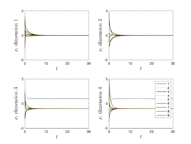
The leftmost subfigure in Figure 4 demonstrates that bipartite consensus is indeed achieved on network as predicted by Theorem 3.8. The simulation result in Figure 5 also shows that the bipartition occurs between and , and the agents converge to .
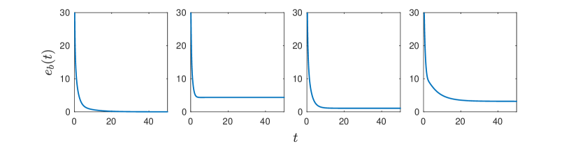
Example 4.2.
In Example 4.1, we can modify the structure or weight matrices of to construct a network that violates only one of the three conditions. The other three subfigures of Figure 4 depict the trajectory of on modified networks and where Condition (1) or Condition (3) or Condition (4) is not met, showing that bipartite consensus is not achieved.
Network , as depicted in Figure 2, also has two continents on and . The two continents are connected by a semidefinite path . The semidefinite edges have the following weights: , , , , where
We then check each assumption and condition. Assumption 1 holds as there exists a unique NBS between and . Condition (1) is violated because the semidefinite path is characterized by equation (I) in Lemma 3.6, while , which intersects nontrivially with . Conditions (2) and (3) apparently hold, while Condition (4) does not apply to this case as there is no edge on the semidefinite path belonging to the NBS. Figure 4 shows that by failing Condition (1) alone, network does not achieve bipartite consensus.
Network has the same structure as network , but changes the weight matrix of edge to . This gives and violates Condition (3) on semidefinite path . One can check that Assumption 1 and Conditions (1), (2), (4) are still satisfied. Figure 4 indicates that bipartite consensus is not achieved on network .
Network , as illustrated in Figure 3, also has the same structure as network , but assigns and . The semidefinite edges have the following weights: , , , , , , , . The unique NBS of is then , with , . One can check that Assumption 1 and Conditions (1), (2), (3) hold. For Condition (4), , but the bases of and , i.e.,
and the basis of , i.e.,
are linearly dependent. In this case, Figure 4 shows that bipartite consensus is not achieved on network .
These additional examples substantiate that the sufficient conditions presented in Theorem 3.8 are not overly conservative.
Remark 4.3.
Here we make a comparison between Theorem 3.8 and Theorem 4 in [20]. Much alike Theorem 3 in [11], Theorem 4 in [20] proposes a sufficient condition to decide if an agent can achieve bipartite consensus with respect to an agent of a continent, or “merge” with it, given the various paths connecting them. Therefore by applying this criterion to all agents outside the continent, one can determine if an overall bipartite consensus can be achieved.
The main idea of both sufficiency theorems in [20] and [11] is that all the connecting paths between and should have trivial intersection of null spaces, i.e., , so that the agents only yield or . In the case of where agents 4 and 5 naturally form consensus as part of a continent, Theorem 4 of [20] would take into account paths , and to verify if agent 2 will merge into the cluster . However, it is obvious that as edges , and all have the same null space to their weight matrices, despite that indeed forms a cluster as indicated in Figure 5.
This comparison indicates that Theorem 3.8 extends previous work by relaxing the requirement for the null spaces of connecting paths to intersect trivially. In fact, as is the Minkowski sum of the null spaces of its weight matrices, for there to be , the options for the semidefinite weight matrices on different paths easily run out when has many paths to reach . Therefore, though not explicitly stated as conditions, strict topological constraints on the semidefinite paths are implied in existing results. Meanwhile, our result offers more flexibility regarding network structure, such as the number and length of semidefinite paths, to achieve bipartite consensus.
5 Concluding Remarks
This work investigates sufficient conditions for achieving bipartite consensus on weakly connected matrix-weighted networks. Recognizing the difference between connections weighted by definite and semidefinite matrices, we first introduce the concept of a “continent” – a subgraph of the network spanned by a positive-negative tree that preserves its bipartite convergence regardless of the configuration of the rest of the graph. Consequently, sufficient conditions for achieving bipartite consensus on the entire network are presented, allowing continents to be connected via the semidefinite paths. Finally, the simulation results illustrate how to verify the proposed conditions and demonstrate that the sufficient conditions are not overly conservative.
Proof for Theorem 3.8.
Proof:
Due to Assumption 1 which states that has a unique NBS, we have established in Lemma 3.5 that agents on each continent converge bipartitely to . Moreover, due to Condition (1) and Lemma 3.6, bipartite consensus is achieved for agents from different continents as well. The ambiguity rests with the agents on the semidefinite paths that bridge the continents, for which we introduce Conditions (2) – (4).
A formal statement of Condition (2) is given as follows. Assume there are two semidefinite paths between continents where and , then we allow and/or without making it a necessity, but the rest of the path should be node-independent which means .
We would first consider the scenario where there is only one semidefinite path between two arbitrary continents, then extend to the general situation of having multiple paths.
Scenario 1:
Assume that there is only one semidefinite path between arbitrary continents . According to Proposition 2.10, Assumption 1 guarantees that is included in the solution space for where specifies the bipartition given by ; we will prove that the columns of actually span the solution space by solving (3) for . For the rest of the proof, we employ to indicate the bipartition of the agents that are on the semidefinite path given by the NBS. The sign pattern of conforms that of , i.e., when and denote the same agent.
For , since and converge bipartitely under Assumption 1 and Condition (1), there is . We denote this solution for the end points as the null space of some matrix , that is,
To simplify the notation, we assign , and its sign as . Then , . Also, denote for . Evaluate equation (3) for the agents on , there is
| (6) | ||||
Case 1: When , the bipartition of respects that of the NBS, which gives . Then after elementary column operations, can be turned into
| (7) |
where , , stands for the zero matrix. It is easy to see that is a solution of (6), and that if is of full rank, the nullity of in (6) is equal to that of , then under the constraints of , the nodes can only converge to . We then check if under Condition (3), there is
It is known that
| (8) |
where is the Moore-Penrose inverse of , and since , we have and . Therefore if has , we have the desired conclusion. Notice that
let and , one can check that for , take the -th row block for example,
which means , therefore . Suppose there exists such that and Equation is written as
where , which is equivalent to have for , meanwhile requires that for . However, the summation
implies that the nonzero ’s are linearly dependent which contradicts Condition (3). We are then left with and . Therefore and the asymptotic values of the agents on are in .
Case 2: If , it is easy to see that has exactly one edge in the NBS because it is node-independent. In this case, the bipartition of does not respect that of the NBS and we have , of (6) instead becomes equal in rank to
| (9) |
To deal with the rank of , suppose , first one could check that
| (10) |
where . denotes the NBS’s partition of which is not respected by the signs of their connecting weights at . This demands for , thus the convergence space for the agents will further take intersection with . Here we have
Instead of directly computing with (8), we now take a different approach by identifying
| (11) |
for block matrix , and partitioning as where , . The eigenvectors that span are readily obtained as the columns of
| (12) | ||||
within which we can find eigenvectors for that are for . As of now, we have shown the dimension of to be no less than as in eqn. (10). Suppose has any other eigenvector as a linear combination of (12), i.e., where , , , , and are not all zeros. Then Conditions (3) and (4) guarantee that such vectors do not exist. We have now proven that eqn. (10) is in fact
Scenario 2:
We now consider multiple semidefinite paths between and , i.e. , eqn. (6) is evaluated for every while the agents of the continents are further bound by the bipartite relation , , . It is then convenient to formulate these relations with the block matrix
| (13) |
for all the agents of and , where correspond to the constraints imposed by , and corresponds to the bipartite relation that couples the equations of the semidefinite paths. The overall solution of eqn. (13) is then found in the intersection of the null spaces of the blocks. As we have derived where or for each semidefinite path, and there is Condition (1) to guarantee the solution of the continents, it is easy to show that the agents of the continents and the semidefinite paths must converge bipartitely.
For the entire system where several continents are interconnected through the semidefinite paths, consider each pair of continents that sets up a constraint which eventually stacks up as . Similarly, we end up taking the intersection of the solution space for the set of constraints, and bipartite consensus is achieved due to the connectivity of the network. In this process, the intersection is taken with for all which means the agents’ states converge to . ∎
Claim .1.
Suppose Assumptions 1 holds. If Conditions (1) and (2) hold, Conditions (3) and (4) must be satisfied to achieve bipartite consensus.
Proof:
This can be validated by finding solutions other than the bipartite one in the Laplacian null space when Condition (3) or (4) does not hold, e.g., assume , then of eqn. (7) does not have full rank as ; applying the row operations inverse to what transforms eqn. (6) to eqn. (7) on this solution, it does not turn out to be bipartite since there are row blocks of both and . Notice that the agents in the middle of the semidefinite paths are not shared with each other, thus even after taking intersection of the solution spaces of the semidefinite paths, this non-bipartite solution does not disappear and stays in the Laplacian null space. The same reason applies to of eqn. (9) when Condition (3) does not hold, considering
If Condition (4) does not hold, there exist , , , such that
due to which bipartite consensus is not achieved for agents on the semidefinite path. ∎
References
- [1] C. Castellano, S. Fortunato, and V. Loreto, “Statistical physics of social dynamics,” Rev. Mod. Phys., vol. 81, pp. 591–646, May 2009.
- [2] A. V. Proskurnikov, A. S. Matveev, and M. Cao, “Opinion dynamics in social networks with hostile camps: Consensus vs. polarization,” IEEE Transactions on Automatic Control, vol. 61, no. 6, pp. 1524–1536, 2016.
- [3] F. Dörfler, M. Chertkov, and F. Bullo, “Synchronization in complex oscillator networks and smart grids,” Proceedings of the National Academy of Sciences, vol. 110, no. 6, pp. 2005–2010, 2013.
- [4] M. A. Kamel, X. Yu, and Y. Zhang, “Formation control and coordination of multiple unmanned ground vehicles in normal and faulty situations: A review,” Annual Reviews in Control, vol. 49, pp. 128–144, 2020.
- [5] A. Tahir, J. Böling, M.-H. Haghbayan, H. T. Toivonen, and J. Plosila, “Swarms of unmanned aerial vehicles a survey,” Journal of Industrial Information Integration, vol. 16, p. 100106, 2019.
- [6] G. Liu, L. Chen, K. Liu, and Y. Luo, “A swarm of unmanned vehicles in the shallow ocean: A survey,” Neurocomputing, vol. 531, pp. 74–86, 2023.
- [7] R. Olfati-Saber and R. M. Murray, “Consensus problems in networks of agents with switching topology and time-delays,” IEEE Transactions on Automatic Control, vol. 49, no. 9, pp. 1520–1533, 2004.
- [8] C. Altafini, “Consensus problems on networks with antagonistic interactions,” IEEE Transactions on Automatic Control, vol. 58, no. 4, pp. 935–946, 2012.
- [9] A. Jadbabaie, J. Lin, and A. S. Morse, “Coordination of groups of mobile autonomous agents using nearest neighbor rules,” IEEE Transactions on Automatic Control, vol. 48, no. 6, pp. 988–1001, 2003.
- [10] S. E. Tuna, “Synchronization under matrix-weighted laplacian,” Automatica, vol. 73, pp. 76–81, 2016.
- [11] M. H. Trinh, C. Van Nguyen, Y.-H. Lim, and H.-S. Ahn, “Matrix-weighted consensus and its applications,” Automatica, vol. 89, pp. 415 – 419, 2018.
- [12] L. Pan, H. Shao, M. Mesbahi, Y. Xi, and D. Li, “Bipartite consensus on matrix-valued weighted networks,” IEEE Transactions on Circuits and Systems II: Express Briefs, vol. 66, no. 8, pp. 1441–1445, 2019.
- [13] J. L. Ramirez, M. Pavone, E. Frazzoli, and D. W. Miller, “Distributed control of spacecraft formation via cyclic pursuit: Theory and experiments,” in 2009 American Control Conference, 2009, pp. 4811–4817.
- [14] S. Zhao and D. Zelazo, “Localizability and distributed protocols for bearing-based network localization in arbitrary dimensions,” Automatica, vol. 69, pp. 334–341, 2016.
- [15] B.-H. Lee and H.-S. Ahn, “Distributed formation control via global orientation estimation,” Automatica, vol. 73, pp. 125–129, 2016.
- [16] H. Hong and S. H. Strogatz, “Kuramoto model of coupled oscillators with positive and negative coupling parameters: An example of conformist and contrarian oscillators,” Phys. Rev. Lett., vol. 106, p. 054102, Feb 2011.
- [17] J. Hu and H. Zhu, “Adaptive bipartite consensus on coopetition networks,” Physica D: Nonlinear Phenomena, vol. 307, pp. 14–21, 2015.
- [18] C. Zong, Z. Ji, L. Tian, and Y. Zhang, “Distributed multi-robot formation control based on bipartite consensus with time-varying delays,” IEEE Access, vol. 7, pp. 144 790–144 798, 2019.
- [19] H. Su, J. Chen, Y. Yang, and Z. Rong, “The bipartite consensus for multi-agent systems with matrix-weight-based signed network,” IEEE Transactions on Circuits and Systems II: Express Briefs, 2019.
- [20] C. Wang, L. Pan, H. Shao, D. Li, and Y. Xi, “Characterizing bipartite consensus on signed matrix-weighted networks via balancing set,” Automatica, vol. 141, p. 110237, 2022.
- [21] S. E. Tuna, “Synchronization of small oscillations,” Automatica, vol. 107, pp. 154–161, 2019.
- [22] H.-S. Ahn, Q. V. Tran, M. H. Trinh, M. Ye, J. Liu, and K. L. Moore, “Opinion dynamics with cross-coupling topics: Modeling and analysis,” IEEE Transactions on Computational Social Systems, vol. 7, no. 3, pp. 632–647, 2020.