Development of a conditional diffusion model
to predict process parameters and microstructures
of dendrite crystals of matrix resin based on mechanical properties
Abstract
In this study, we develop a conditional diffusion model that proposes the optimal process parameters, such as processing temperature, and predicts the microstructure for the desired mechanical properties, such as the elastic constants of the matrix resin contained in carbon fiber reinforced thermoplastics (CFRTPs). In CFRTPs, not only the carbon fibers but also the matrix resin contribute to the macroscopic mechanical properties. Matrix resins contain a mixture of dendrites, which are crystalline phases, and amorphous phases even after crystal growth is complete, and it is important to consider the microstructures consisting of the crystalline structure and the remaining amorphous phase to achieve the desired mechanical properties. Typically, the temperature during forming affects the microstructures, which in turn affect the macroscopic mechanical properties. The training data for the conditional diffusion model in this study are the crystallization temperatures, microstructures and the elasticity matrix. The elasticity matrix is normalized and introduced into the model as a condition. The trained diffusion model can propose not only the processing temperature but also the microstructure when Young’s modulus and Poisson’s ratio are given. The capability of our conditional diffusion model to represent complex dendrites is also noteworthy.
keywords:
conditional diffusion model , extended finite element method , phase-field method , dendrite , matrix resin[inst1]organization=Graduate School of Science and Technology, Keio University,addressline=3-14-1, city=Hiyoshi, Kohoku-ku, Yokohama, postcode=223-8522, state=Kanagawa, country=Japan
[inst2]organization=Department of Aeronautics and Astronautics, The University of Tokyo,addressline=7-3-1, city=Hongo, Bunkyo-ku, postcode=113-8656, state=Tokyo, country=Japan
[inst3]organization=National Institute of Advanced Industrial Science and Technology,addressline=1-1-1, city=Umezono, Tsukuba, postcode=305-8568, state=Ibaraki, country=Japan
[inst4]organization=Department of Mechanical Engineering, Keio University,addressline=3-14-1, city=Hiyoshi, Kohoku-ku, Yokohama, postcode=223-8522, state=Kanagawa, country=Japan
1 Introduction
Carbon fiber reinforced thermosetting plastics (CFRTSs) and carbon fiber reinforced thermoplastics (CFRTPs) have excellent light weight and strength [1]. These materials are increasingly applied to structural components of aircraft and automobiles [2, 3]. However, aircraft and automobiles have different requirements. Therefore, it is important to develop materials with the desired properties for the application. CFRTSs have the property of stiffening upon heating and not returning to its original state, whereas CFRTPs have the property of stiffening upon cooling and softening again upon heating. CFRTSs have been applied to many structures, but the material and molding costs are high. In addition, it is difficult to recycle CFRTSs once stiffened, which poses a disposal problem [4, 5]. On the other hand, CFRTPs have been attracting attention as a sustainable material due to its low molding cost and recyclability [6]. In CFRTPs, the mechanical properties depend not only on the carbon fibers, but also on the matrix resin used as the base material. The thermoplastic resins used in CFRTPs are crystalline resins, such as polyphenylene sulfide (PPS) and polyether ether ketone (PEEK), which have significant rigidity [7, 8]. Crystalline and amorphous phases are mixed in matrix resins, and it is important to consider the microstructures consisting of the crystalline structure and the remaining amorphous phase to achieve the desired mechanical properties. As crystallization progresses, matrix resins become stronger and stiffer. This increases the overall strength and stiffness of the composite. On the other hand, the amorphous phase contributes to the ductility of the composite. Therefore, it is important to consider the balance of crystalline and amorphous phase and their arrangement.
In this study, we focus on PPS, a thermoplastic resin with low costs. PPS has a mixture of crystalline and amorphous phases even when the crystals are fully grown. It produces dendritic crystals called dendrites during solidification [9]. Process parameters such as temperature during forming and cooling rate affect the microstructure, which in turn affects the macroscopic mechanical properties [10, 11, 12, 13, 14, 15, 16]. Thus, a method of predicting the mechanical properties of resins is required. To improve the mechanical properties of composites such as CFRTP and CFRTS, various experiments have been tried [17, 18, 19, 20, 21, 22, 23]. It is important to investigate the properties of materials through experimentation. On the other hand, it is very expensive to try different conditions in the experiment. To solve this problem and to develop materials efficiently, simulation has been introduced.
Higuchi et al. [24] and Takashima et al. [25] developed a multiphysics analysis method for crystalline thermoplastic resins that links the forming conditions, the microstructure and the macroscopic mechanical properties. Crystallization analysis was performed by using the phase-field method [26, 27, 28, 29]. The homogenization analysis [30] of PPS, a crystalline thermoplastic resin, was conducted by using the extended finite element method (XFEM) [31, 32, 33, 34, 35, 36]. PPS was characterized to identify the parameters necessary for crystallization analysis. The simulation results were validated by comparing them with experimental data. The details of their studies [24, 25] are as follows. They measured properties such as the glass transition temperature, crystallization temperature and melting point by differential scanning calorimetry (DSC). Moreover, they examined the relationship between the processing temperature and the mechanical properties by tensile tests. The phase-field model they developed reproduced various types of nucleation and polycrystal growth. Conventional methods for dendrite simulation divide the analysis domain into cells and discretely assign states to them, e.g., the cellular automata [37, 38, 39, 40] and Monte Carlo [41, 42] methods. The other method represents the interface by connecting discrete points such as the front-tracking method [43, 44, 45]. Higuchi et al. [24] used the phase-field method to describe the crystal growth of dendrites in thermoplastic resins, in terms of the interface movement between two different phases. Then, they performed the homogenization analysis of the obtained microstructures using XFEM to determine the mechanical properties such as Young’s modulus. By comparing the analytical results with the experimental results, it is shown that their proposed method has a certain validity. Their method is limited to forward analysis, and it is not possible to predict the processing temperature or microstructure from the mechanical properties. In addition, machine learning is sometimes used for efficient material development because it takes a long time to try many patterns in a simulation.
In the field of mechanics of materials, machine learning has achieved significant results in the prediction of physical properties [46, 47, 48, 49, 50, 51, 52]. Jadhav et al. [46] proposed a StressD framework for predicting von Mises stress fields of structures based on the denoising diffusion model. They applied the StressD framework to four datasets. The datasets [53, 54] are coarse mesh, fine mesh, sparse and hyperelastic datasets. The coarse mesh dataset has cantilever structures composed of homogeneous and isotropic linear elastic materials. The fine mesh dataset has 50,000 data points sampled from the coarse mesh dataset. The sparse dataset has data randomly sampled from of the stress field in the material domain. The hyper elastic dataset has distinctive data based on a two-dimensional (2D) hyperelastic problem. The StressD framework has two models: the denoising diffusion model and auxiliary network. The denoising diffusion model generates a normalized stress map on the basis of a given geometry and other conditions. The auxiliary network determines the scaling information required to un-normalize the generated stress map. Compared with the conventional method of finite element analysis (FEA), the computational cost of the StressD framework is significantly reduced and the von Mises stress field is accurately predicted. In this way, machine learning contributes to the reduction of computational cost by using it for the prediction of physical properties.
In material development, machine learning has also contributed markedly [55, 56, 57, 58, 59, 60, 61, 62, 63, 64, 65]. Kumar et al. [55] developed a machine learning strategy for the inverse design of spinodoid topology. This strategy enables the creation of metamaterials with specific mechanical properties. Bastek et al. [56] developed a method for the inverse design of nonlinear mechanical metamaterials using a video denoising diffusion model. The video denoising diffusion model is trained on full-field data of periodic stochastic cellular structures. They showed that the model can predict and tune the nonlinear deformation and stress response under compression in the large-strain regime. Veasna et al. [57] developed a Pareto-based multiobjective machine learning method for efficiently identifying parameters of crystal plasticity models. The model parameters are identified for two steel alloys, the dual-phase (DP) steel DP780 and the stainless steel (SS) SS316L. Their method greatly reduces the number of expensive black-box function runs and allows the parameters to be accurately specified. Hiraide et al. [58] developed a framework for forward analysis to predict Young’s modulus from the phase-separated structure of polymer alloys and for inverse analysis to predict the structure from Young’s modulus. Forward analysis uses convolutional neural networks (CNNs) [66, 67]. For inverse analysis, random search is applied to the combined generative adversarial network (GAN) [68, 69] and CNN model. Moreover, Hiraide et al. [59] proposed a framework for designing material structures based on macroscopic properties. They use the results of the analysis of the two-dimensional phase separation structure of diblock copolymer melts as structural data. The stress data are obtained by FEA. The framework consists of a deep learning model that generates structures and a model that predicts the physical properties of the structures. It generates structures with desired physical properties using random search.
The denoising diffusion model, one of the machine learning models, is increasingly used in the design of materials [64]. Lee and Yun [64] proposed a framework for reconstructing anisotropic microstructures from 2D micrographs. They use the dataset from experimentally obtained 2D micrographs. The materials are a lithium-ion battery separator [70], carbon fiber composites [71] and lithium-ion nickel manganese cobalt (NMC) cathode samples [72]. To train conditional diffusion-based generative models (DGMs) for 2D-to-three-dimensional (3D) reconstruction, 2D micrographs from three orthogonal planes of each material are randomly sampled from the open-access tomographic data [70, 71, 72]. In this framework, 3D microstructures are generated from multiple 2D datasets using conditional DGMs. They validate the 3D reconstructed anisotropic microstructure samples by evaluating spatial correlation functions and physical material behavior.
Thus, machine learning has been used to predict physical properties and develop materials. Methods of predicting mechanical properties from microstructures and microstructures from mechanical properties have been developed. However, there is no scheme for proposing process parameters and material microstructures related to how materials should be made. If process parameters such as processing temperature and cooling rate are proposed to produce materials with the desired mechanical property, it will be possible to develop materials efficiently by eliminating the need for trial-and-error experiments using different parameters.
The purpose of this study is to develop a conditional diffusion model that proposes the optimal processing temperature and predicts the microstructure on the basis of the desired Young’s modulus and Poisson’s ratio. As an example, we analyzed PPS, a thermoplastic resin that is the base material of CFRTP, assuming composite applications.
This paper is organized as follows. The details of the methods for crystal growth, homogenization analysis using XFEM and conditional diffusion model are described in Section 2. The results and discussion of this study are given in Section 3. Finally, the conclusions are presented in Section 4.
2 Methods
2.1 Crystal growth
This study introduces two models for the crystal nucleation and growth. The models are used to generate the data of microstructures depending on the temperature. In this study, the crystallization and ambient temperatures are the same owing to the assumption of isothermal forming. Therefore, we consider the crystallization temperature as a parameter that can be specified in the process.
2.1.1 Crystal growth by phase-field method
The phase-field method is a method of describing the movement of surfaces by solving the time evolution equation of the phase-field variable . In this method, the dimensionless variable , which varies between and where for the crystalline phase and for the amorphous phase, is used to show the spatial distribution of the crystalline and amorphous phases.
The crystal growth is described by the Allen–Cahn and heat conduction equations respectively as follows [29]:
| (1) |
| (2) |
where is the phase-field variable, is the time, is the phase-field mobility, is the free energy of the system, is the field temperature, is the thermal diffusivity, is the latent heat and is the specific heat at a constant pressure. The total free energy of the system is expressed as follows [27]:
| (3) |
where is the double-well potential and is the gradient energy density. Here, , , and are respectively expressed as
| (4) |
| (5) |
| (6) |
| (7) |
where is the height of the energy barrier, is the dimensionless temperature and is the coefficient of interface energy gradient. The constants are set as and . From Eq. (7), we find that the crystal growth depends on the crystallization temperature .
2.1.2 Formation of crystal nuclei
For the modeling of crystal nucleation, in this study, we introduce the model proposed by Pantani et al. [73] as
| (8) |
where is the nucleation rate, is the nucleation density, is the field temperature, is the time, is a constant independent of temperature, is the temperature at which molecular motion stops completely, and are nucleation rate parameters and is the melting point obtained at a particular crystallization temperature . The Hoffman–Weeks plot shows the crystallization temperature on the horizontal axis and the melting point on the vertical axis. DSC [74] gives the melting point from the starting temperature of the melting peak of the DSC curve. Thus, nucleation depends on the crystallization temperature . In Eq. (8), , where is the crystallization temperature (ambient temperature), is the slope of the approximate line between the crystallization temperature and the melting point obtained from the Hoffman–Weeks plot, and is the intercept of the line [75]. Although this model assumes homogeneous nucleation in which the nucleation occurs stochastically on the basis of nucleation rate, the actual nucleation is heterogeneous because, for example, unknown inclusions can accelerate the nucleation. To consider this effect, a few initial nuclei are initially introduced in this study.
2.1.3 Generation of crystal microstructure by the phase-field method
To generate the microstructure of matrix resins for machine learning, we use the phase-field method. The size of a nucleus is equal to one grid for simplicity. The analysis is performed at three crystallization temperatures: 160 ∘C, 180 ∘C and 200 ∘C. Table 1 shows the conditions used in the analysis by the phase-field method. The condition parameters in the phase-field method are obtained from the references [29, 76].
| Number of calculation steps | 20,000 |
|---|---|
| Number of grid points | |
| Crystallization temperature | 160 ∘C, 180 ∘C, 200 ∘C |
| Temperature at maximum crystallization rate | 180 ∘C |
| Glass transition temperature | 100 ∘C |
| Number of initial nuclei | 2 |
| Boundary condition | Periodic boundary condition |
2.2 Homogenization analysis using XFEM
2.2.1 XFEM
The elasticity matrix used as the condition of the diffusion model is obtained by homogenization analysis using XFEM for matrix resins generated by the phase-field method. At the interface between the crystalline and amorphous phases, the strain is discontinuous and the local modification of the interpolation function allows accurate approximation. The nodes for XFEM are generated on the basis of the differentially discretized grid for the phase-field method and the triangular elements are generated by dividing the square grid into two parts. In addition, subelements are introduced for elements containing interfaces to integrate discontinuous functions with high accuracy. In XFEM, the displacement is expressed as
| (9) |
where is the node, is the shape functions, is the coordinates, is the vector of node displacement, is the enriched function to be introduced locally in the interpolating function and is the nodal degree of freedom for the basis function added by the enriched function. The ramp function proposed by Moës et al. [77], which is introduced as an enriched function, can express the continuity of displacement and its derivative, which is the discontinuity of strain, and is expressed as
| (10) |
where is the level set function at node and is expressed in terms of the phase-field variable as
| (11) |
Thus, , which means that the phase-field variable , is recognized as the interface between the crystalline and amorphous phases.
2.2.2 Elasticity matrix calculated by homogenization analysis using XFEM
In this study, we use microstructure analysis tools that combine XFEM and the homogenization method [35]. We obtain the stress distribution using XFEM. Then, we obtain the mean stress by the homogenization method assuming a homogeneous body. The key-degree-of-freedom method proposed by Li et al. [78], which imposes boundary conditions via the additional degree of freedom apart from the model mesh, makes it easier to treat macroscopic stresses and strains. In this study, we use the nonlinear XFEM code combined with phase-field simulation [36].
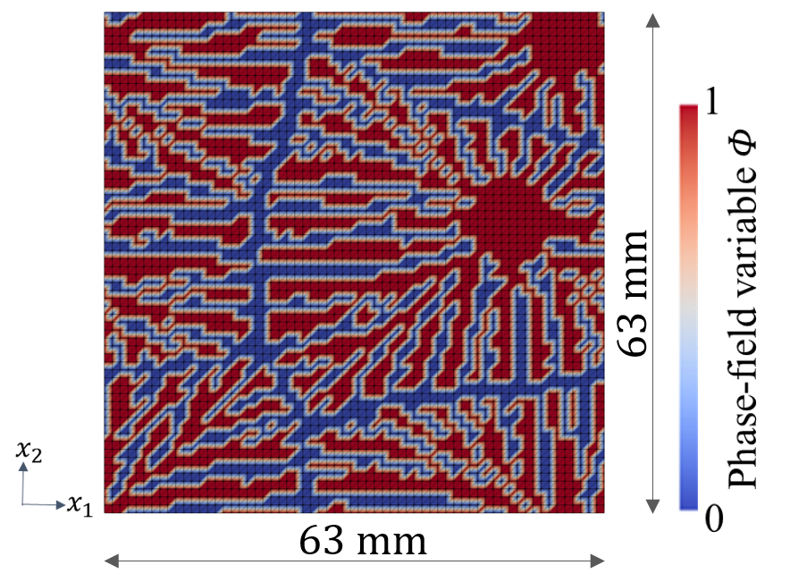
Table 2 shows the conditions for XFEM. The analysis size of XFEM is shown in Fig. 1. The length order of this phase-field method is nondimensionalized. Since dimensions are not relevant in homogenization analysis using XFEM, the dimensionless model is directly loaded into a program with an unit system and solved on the order. Table 3 shows the physical properties of the PPS used for XFEM. The elasticity matrix is obtained by the identified Young’s modulus and Poisson’s ratio [24, 25] (A).
| Size of analysis area | |
|---|---|
| Incremental time | 1.0 s |
| Newton–Raphson method convergence index | 0.1 |
| Boundary condition | Periodic boundary condition |
2.3 Conditional diffusion model
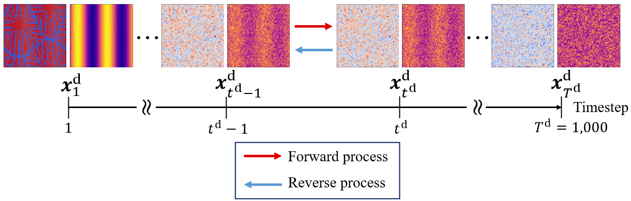
In this study, we employ a diffusion model for predicting the process parameters and the microstructures for the desired mechanical properties. The diffusion model [80, 81, 82, 83, 84, 85] was proposed by Sohl-Dickstein et al. [80] and improved as the denoising diffusion probabilistic model (DDPM) by Ho et al. [81]. The model used in this study is DDPM with condition, which is the called conditional diffusion model. The conditional diffusion model consists of the forward and reverse processes, as shown in Fig. 2. In the forward process, Gaussian noise is added to the images at each timestep using Markov chains. The forward process is defined as follows [81]:
| (12) |
| (13) |
where is the data, is the noise, are the latents, is the arbitrary timestep, is the total number of timesteps for noise addition and removal, is the stochastic process of the forward process, is the normal distribution, are the variance schedule, is the mean and is the variance. In the reverse process, U-Net is used to remove the noise at each timestep. During training, the model learns parameters for generating images from noise by repeatedly adding to and removing noise from images in the forward and reverse processes. The reverse process is defined as follows [81]:
| (14) |
| (15) |
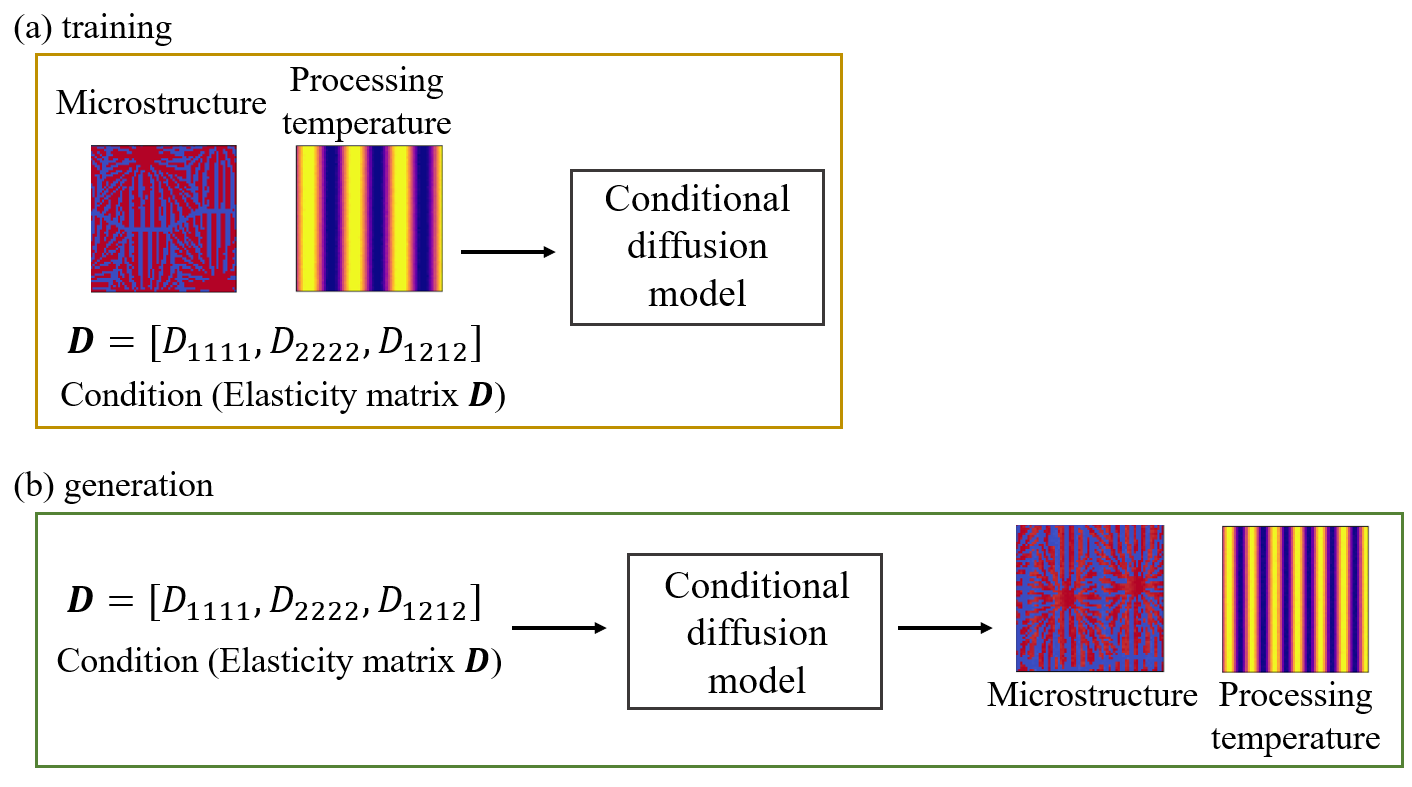
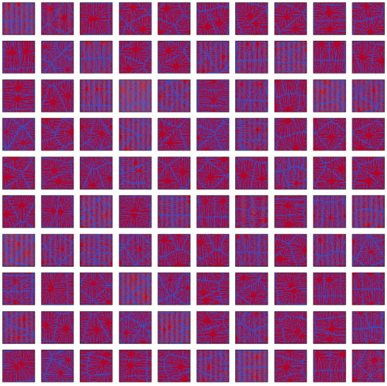
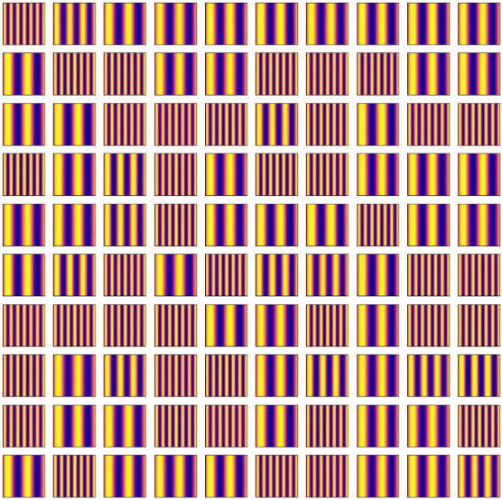
where is the stochastic process of the reverse process, is the stochastic process of the reverse process using the neural network and is parameterized as a neural network. As shown in Fig. 3, the training data are the microstructures of matrix resins generated by the phase-field method, the processing temperatures specified in the phase-field analysis and the elasticity matrix obtained by homogenization analysis using XFEM for the microstructure generated by the phase-field analysis. For the training data of processing temperature, we generate image patterns of processing temperature (IPPT). Note that IPPT does not mean the distribution of temperatures, but gives a pattern for temperature conditions.
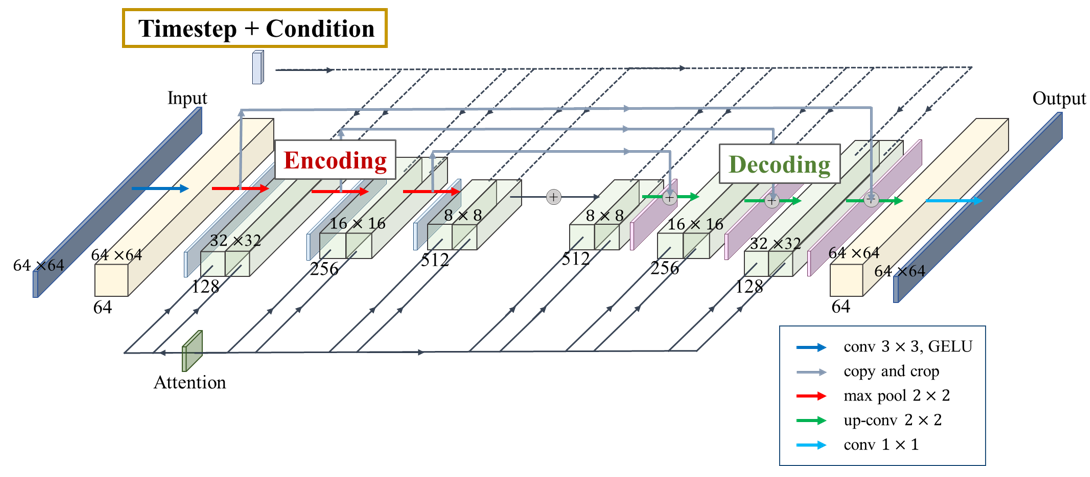
Noise is added to and removed from images of the microstructures and IPPTs. In the process of image generation, only the reverse process of the diffusion model is used to generate images from noise distributions. We use U-Net to remove the noise at each timestep. The U-Net used in this study is the spatiotemporal U-Net (ST-UNet) [86], which includes the time information of noise-adding and noise-removing steps, as shown in Fig. 4 [87]. U-Net is a method developed by Ronneberger et al. [88] for semantic segmentation, in which features are extracted from original images by an encoder and the obtained images are reconstructed in the same size as the original images by a decoder on the basis of the extracted features. Detailed information such as location information is not lost by maintaining feature maps with skip connections at each process. It is possible to change the method of removing for each condition by considering the information of the timestep in the processes of adding and removing noise. In this study, the component of the elasticity matrix is used as the condition. In U-Net, the condition and time information are added to the image at each of the encoding and decoding processes, as shown in Fig. 4. Then, the condition and time information are convolved with the image.
The training data are the microstructures of matrix resins, IPPTs and the elasticity matrix . The microstructures are generated by the phase-field method, IPPT means the temperature specified in the phase-field analysis and the elasticity matrix is obtained by homogenization analysis using XFEM for the microstructures generated by the phase-field method. We employ images of microstructures upon crystal growth completion. Images of the microstructures of dendrites are compressed for use in training machine learning. The mean values of regions are calculated for each analysis grid to be compressed to . In addition, continuous phase-field variables are binarized during compression. Moreover, we perform data augmentation on the microstructures generated by the phase-field method. The rotation, inversion with respect to the axis, inversion with respect to the axis and rotation are conducted for the same elasticity matrix value.
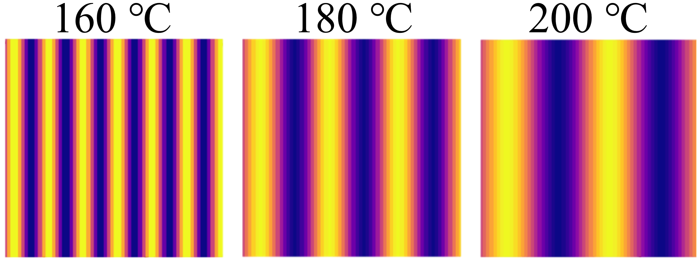
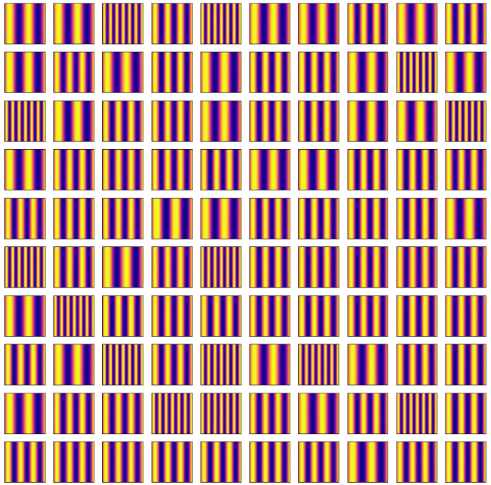
To classify the temperature on the basis of the images, we create different patterns of images of IPPT at each temperature. We specify so that the frequency is a function of the crystallization temperature and to produce the sinusoidal stripe image as IPPT shown in Fig. 5, where is the luminance, is the amplitude, is the frequency, is the abscissa coordinate and is the crystallization temperature. The reason for using sinusoidal stripe images as the training data is that these images can be used for determining the temperature through Fourier transform using the determined frequency. The data of microstructures and IPPT are , for a total of .
The elasticity matrix given as the condition is a vector with three components. The conditions used in training are , and , which are normalized from to . For the diffusion model, the time information during noise addition and removal is important. The model is trained by adding 256-dimensionally expanded conditions to 256-dimensionally expanded time information. Specifically, the original three-component condition values are repeated to extend the dimension, and the extra components are filled with zeros. The time information is extended to 256 dimensions by positional encoding. By adding the condition to the time information, we can change the weight of each condition so that the diffusion model learns a different way to remove noise depending on the condition.
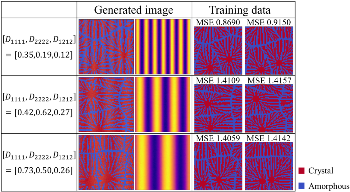
Table 4 shows the number and size of data used for training. To avoid overfitting, we stopped training before an upward trend in the loss of the validation data. By comparing the mean squared errors (MSEs) of the images generated using the trained model and the training data, we confirmed the generalization performance of the model. The value of MSE should be large because we want to generate data that is different from the training data. As shown in Fig. 6, MSE is sufficiently large to show that the generated microstructure is different from the microstructure used for training.
| Number of training data | 13,908 |
|---|---|
| Number of validation data | 1,728 |
| Number of test data | 432 |
| Image size | |
| Minibatch size | 15 |
| Number of epochs | 1,189 |
3 Results and Discussion
3.1 Dataset
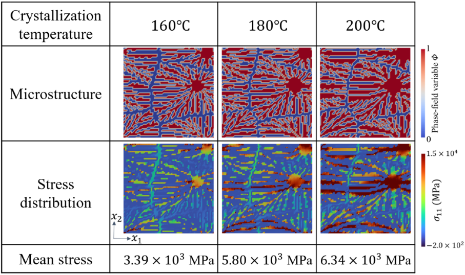
Fig. 7 shows examples of training data of the microstructures generated by the phase-field method, the distribution of the -directional tensile stress and the mean stress obtained by homogenization analysis using XFEM (under the condition of Eq. (17a)). The microstructures indicate that the higher the crystallization temperature, the thicker the crystal chains grow. The stress distribution shows that high stresses are generated near the nuclei toward the direction of the imposed strain. Moreover, increasing the crystallization temperature increases the values of stress distribution and mean stress.
3.2 Validation of proposed processing temperatures and microstructures
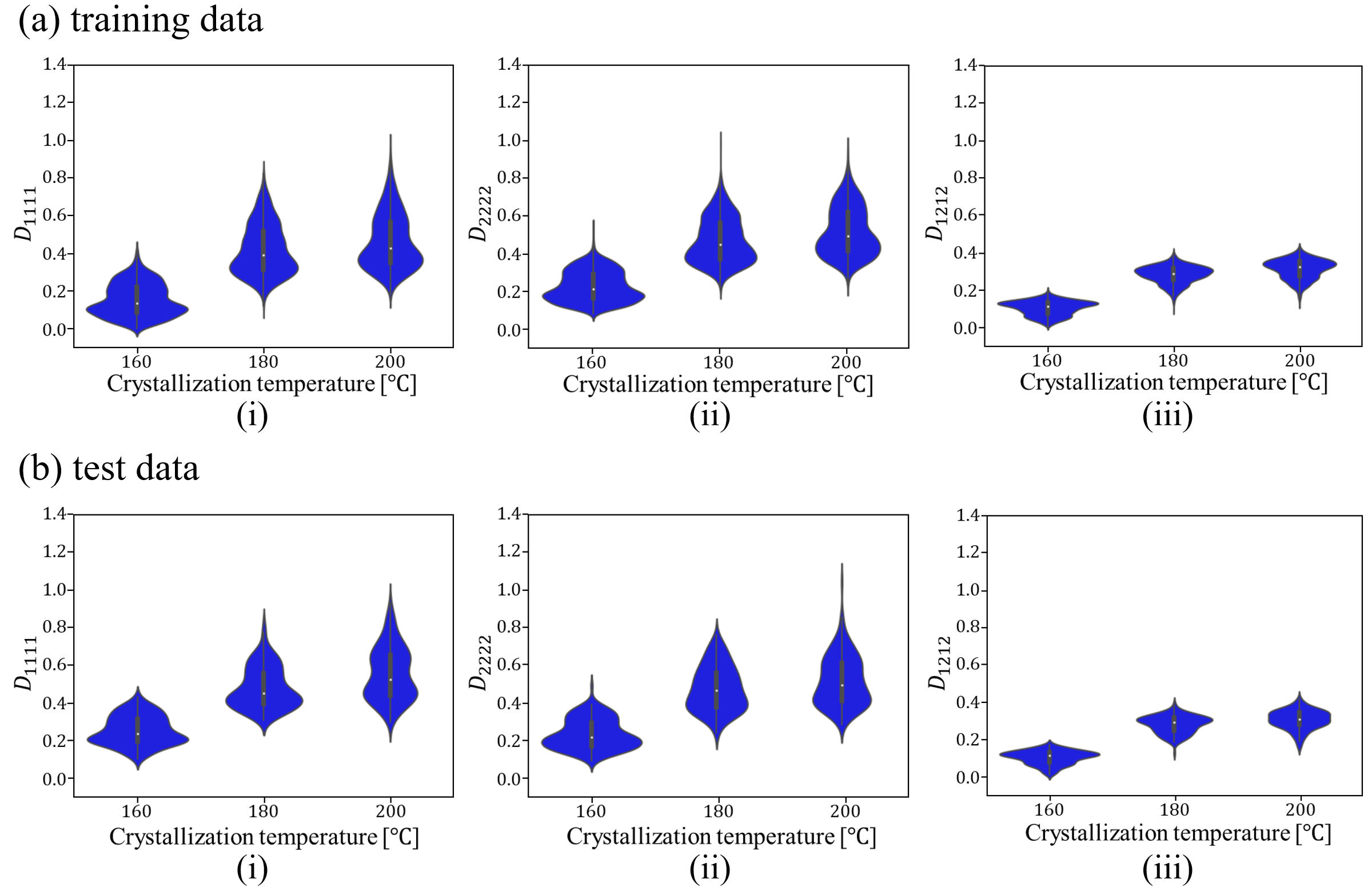
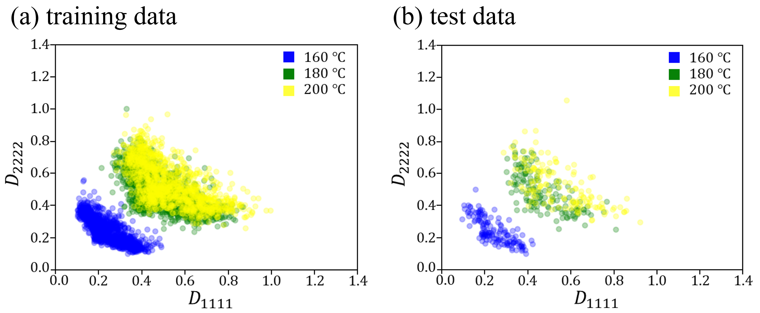
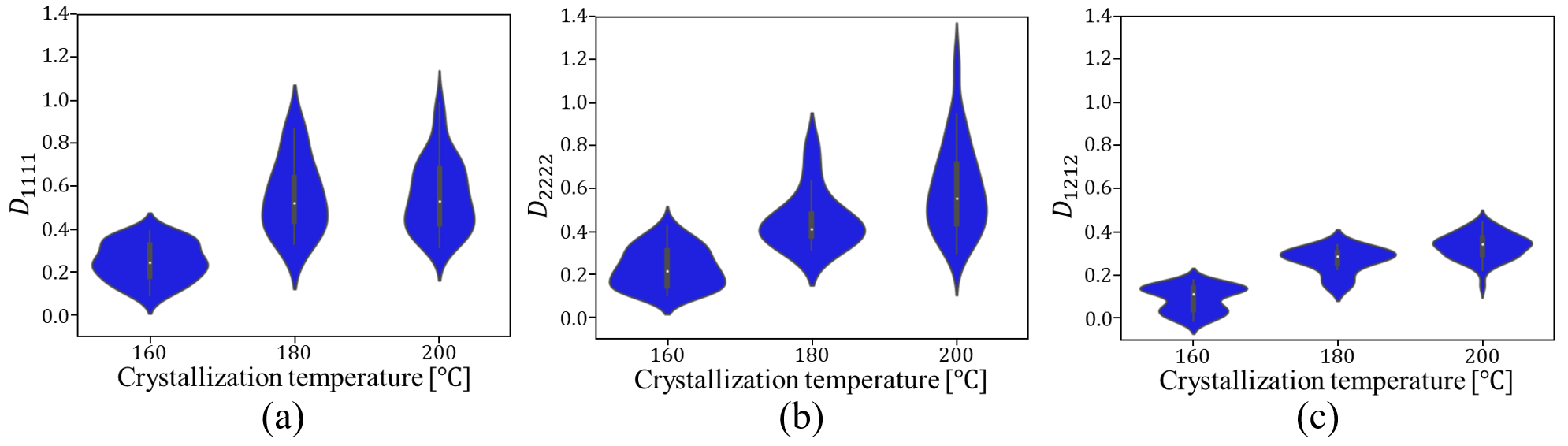
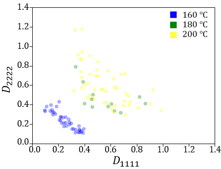
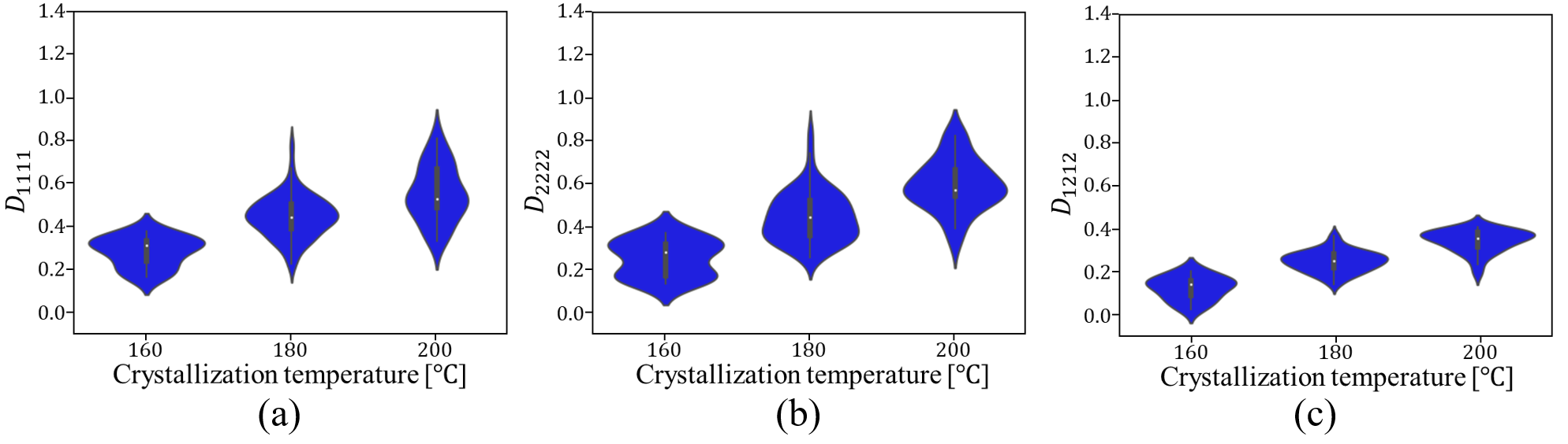
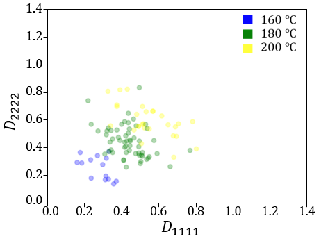
Figs. 8 and 9 show the relationship between the crystallization temperature specified in the phase-field analysis and the elasticity matrix obtained by XFEM for the microstructures generated by the phase-field method for (a) training and (b) test data, respectively. The violin plots in Fig. 8 show the distribution of the data with the horizontal axis for the crystallization temperature and the vertical axis for the value of each component of the elasticity matrix . Each violin plot shows that there is a large amount of data in the bulging part of the plot and a large scatter of data in the vertically long part of the plot. The black rectangle in the plot represents the interquartile range of the box plot, and the white dot at the center represents the median value. Fig. 9 shows scatter plots of on the horizontal axis and on the vertical axis, with different colors indicating the crystallization temperature. These plots show that the higher the crystallization temperature, the larger the value of each component of the elasticity matrix .
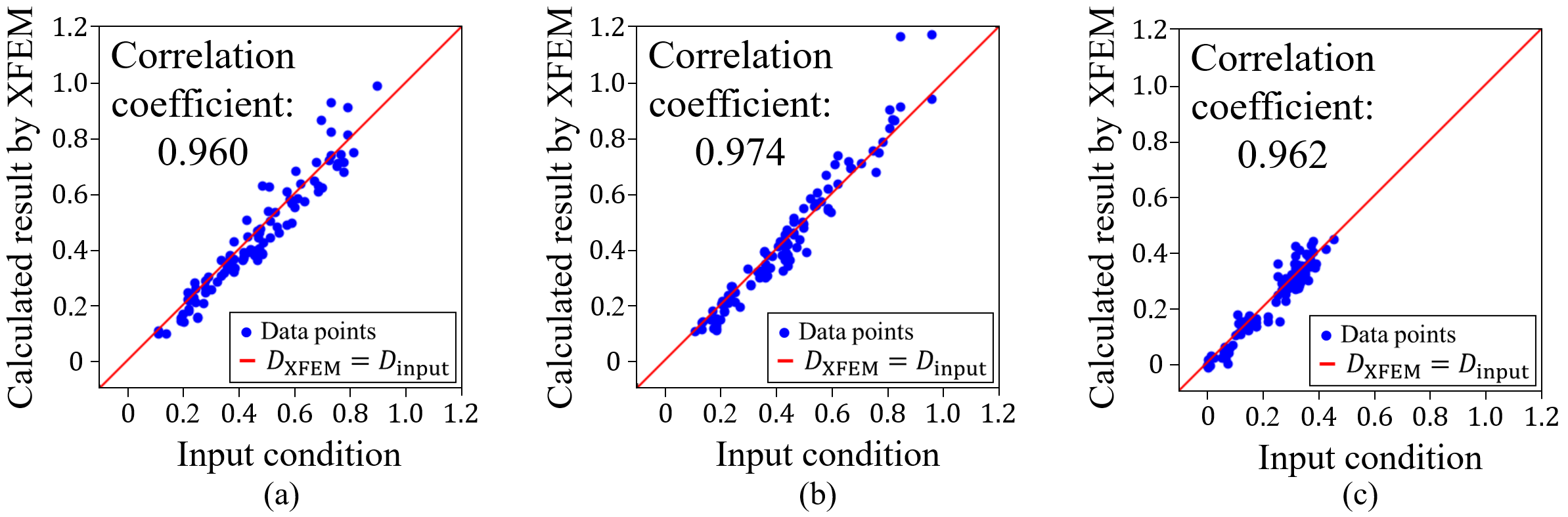
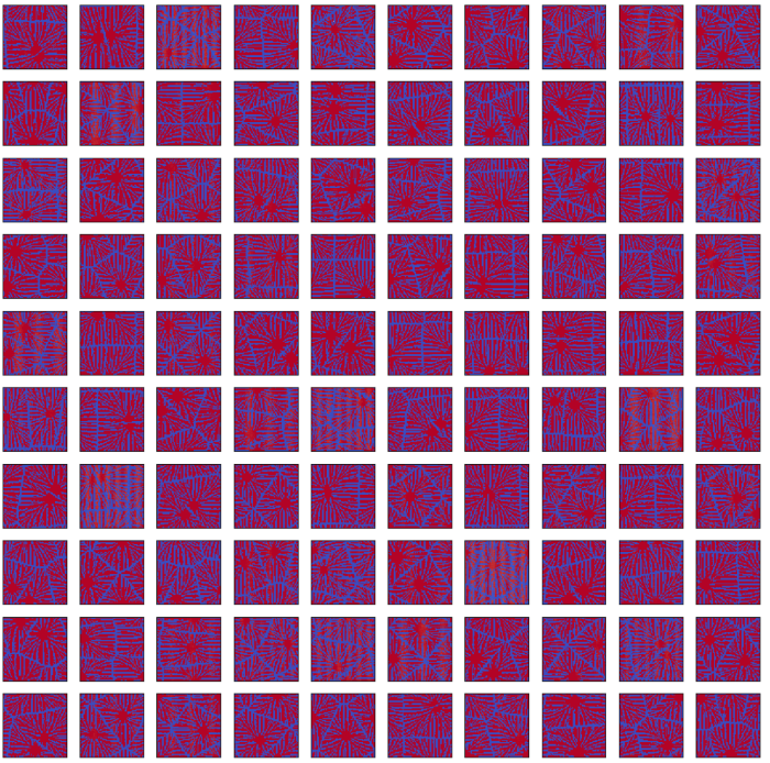
Firstly, we confirmed the trained model by using the condition of the test data. Figs. 10–14 show the results. Fig. 10 shows the generated images of microstructures and Fig. 11 shows the generated images that indicate the processing temperature. Fig. 12 shows the relationship between the proposed temperature and the elasticity matrix obtained by homogenization analysis using XFEM again for the generated microstructure. Fig. 13 is a scatter plot with on the horizontal axis and on the vertical axis, plotted in different colors for different crystallization temperature. From Figs. 12 and 13, the relationship between crystallization temperature and elasticity matrix is generally appropriate because the tendencies of the training data and test data are similar. Fig. 14 compares the values of each component of the elasticity matrix obtained by homogenization analysis using XFEM of the generated microstructure again with the condition given for generation. The red line indicates the ideal situation that the elasticity matrix obtained by homogenization analysis using XFEM for the generated microstructure is equal to the elasticity matrix given as the condition, i.e., when . Where is the element of the elasticity matrix obtained by homogenization analysis using XFEM of the generated microstructure again, is the element of the elasticity matrix given for generation. From the correlation coefficients and each plot, the elasticity matrix obtained by the homogenization analysis using XFEM shows good agreement with the condition given for generation. The correlation coefficients indicate a strong positive correlation, which is considered that the predicted microstructure is appropriate for the given condition.
3.3 Results for conditions not included in the dataset
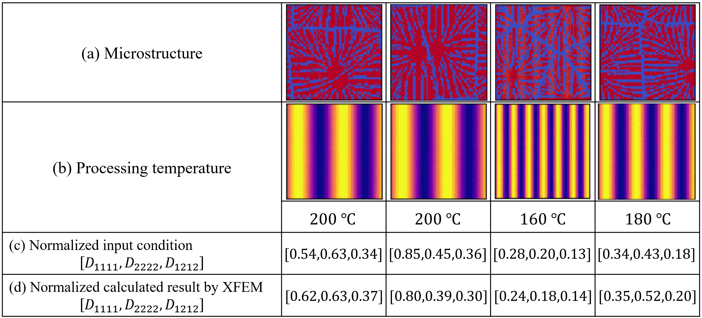
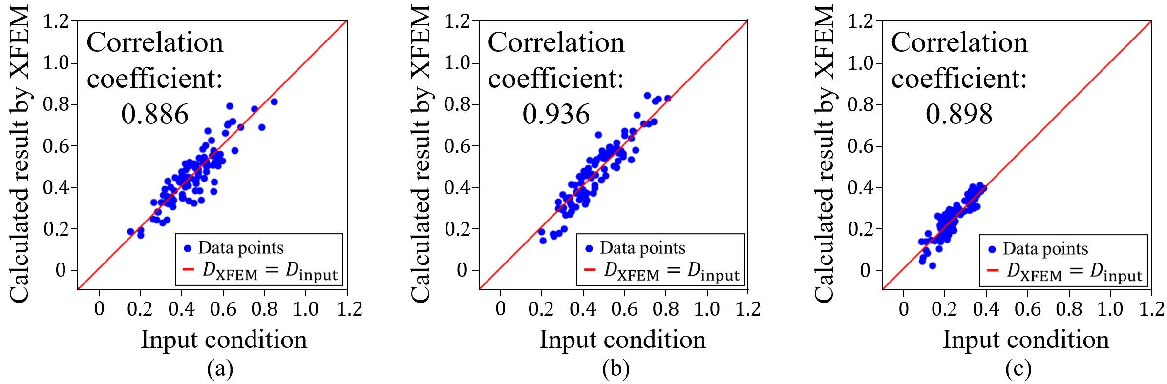
We confirm the results for the conditions not included in the dataset. The results are shown in Figs. 15–20. Fig. 15 shows the generated images of microstructures and Fig. 16 shows the generated images that indicate the processing temperature. Fig. 17 shows the relationship between the proposed temperature and the elasticity matrix obtained by homogenization analysis using XFEM for the generated microstructure. Fig. 18 is a scatter plot with on the horizontal axis and on the vertical axis, plotted in different colors for different crystallization temperatures. Figs. 17 and 18 show that the relationship between crystallization temperature and the elasticity matrix is generally similar to that of the training and test data, even when the data are generated using the conditions not included in the dataset. Fig. 19 shows examples of the generated results. The model developed outputs images of microstructures and IPPTs. Fig. 19 shows (a) the generated microstructures, (b) IPPTs, (c) the conditions and (d) the elasticity matrix values obtained by homogenization analysis using XFEM for the generated microstructure. As shown in Fig. 19(a), the conditional diffusion model can represent the detailed microstructure of dendrite crystals of matrix resins. By homogenization analysis with XFEM to obtain the elasticity matrix for the predicted microstructure, we find that elasticity matrix is close to the condition given for generation. Fig. 20 shows the elasticity matrix for each component. The horizontal axis represents the elasticity matrix obtained by homogenization analysis using XFEM for the generated microstructure, and the vertical axis is the condition given for generation. The correlation coefficients and each plot indicate that the values of elasticity matrix obtained by homogenization analysis using XFEM agree with the condition given for generation with good accuracy. The correlation coefficients imply a strong positive correlation between input condition and calculated result by XFEM, suggesting appropriate microstructure for the given condition.
3.4 Demonstration of the proposed conditional diffusion model
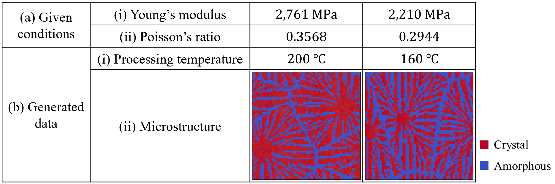
The conditional diffusion model developed in this study can propose the optimal processing temperature and predict the microstructure for given Young’s modulus and Poisson’s ratio. The advantage of this model is that it outputs not only the processing temperature but also the microstructure as images. Fig. 21 shows example of the model demonstration. Fig. 21 shows (a)(i) the specified values of Young’s modulus, (a)(ii) the specified values of Poisson’s ratio, (b)(i) the proposed temperatures and (b)(ii) the predicted microstructures of matrix resins. We train the model with the conditions obtained by homogenization analysis using XFEM on before image compression. Table 5 shows the number and size of data used for training. The relationship between Young’s modulus and Poisson’s ratio and the calculation of the elasticity matrix is described in A. As shown in Fig. 21, 200 ∘C is proposed for a large Young’s modulus of , whereas 160 ∘C is suggested for a small Young’s modulus of . Thus, the results show that the temperature tends to increase with Young’s modulus.
| Number of training data | 13,908 |
|---|---|
| Number of validation data | 1,728 |
| Number of test data | 432 |
| Image size | |
| Minibatch size | 5 |
| Number of epoch | 549 |
4 Conclusions
In this study, we developed a conditional diffusion model that can propose the optimal processing temperature and predict the microstructure for the desired elastic constants. As an example, we analyzed PPS, a thermoplastic resin that is the base material of CFRTP, under the assumption of composite material applications. As a result of using the developed model, the following three were confirmed:
-
1.
By training the pattern that indicates the processing temperature together with the images of the microstructure, the model could predict not only the processing temperature but also the microstructure when the elastic constants were given.
-
2.
The developed model proposed high temperatures with high Young’s modulus. At high temperatures, the predicted crystal structures were obtained with thicker crystal chains.
-
3.
Even when the conditions were not included in the dataset, complicated dendritic patterns whose elastic constants were reasonable were reproduced.
In conclusion, the conditional diffusion model developed in this study can propose the optimal processing temperature and predict the microstructure of matrix resins that satisfies the desired mechanical properties. This study enables us to realize an inverse design that proposes the process parameters related to how the material should be made so as to satisfy the mechanical properties. The model can be extended to composites by including fibers in the analysis. By replacing the training data of microstructure, process temperature and elasticity matrix, this model can be applied to other materials such as CFRTS containing polymer blends with phase-separated structures.
Acknowledgments
This study was partially supported by the Japan Society for the Promotion of Science (JSPS) KAKENHI (Grant Number 22K14489).
Appendix A Homogenization analysis and elasticity matrix
The input data for homogenization analysis using XFEM are phase-field variables, grid information, material properties and boundary conditions. The relationship between stress and strain is expressed as
| (16) |
where and are the normal stress, is the shear stress, , , , , and are the components of the elasticity matrix , and are the normal strain and is the shear strain. For each component of shear strain, the engineering shear strain , which is twice the amount of the shear component of the strain tensor, is used. By homogenization analysis using XFEM, we obtain , and by applying unit strain in the following three patterns:
| (17a) | |||
| (17b) | |||
| and | |||
| (17c) | |||
The mean stress distribution in each direction is written as macroscopic stress in the out-file output of homogenization analysis using XFEM. Since we provide unit strains, is when Eq. (17a) is substituted into Eq. (16), is when Eq. (17b) is substituted into Eq. (16) and is when Eq. (17c) is substituted into Eq. (16).
Owing to the assumption of isothermal forming as the simplest process condition, Young’s modulus and Poisson’s ratio are expressed using the mean values of and :
| (18) |
| (19) |
References
- [1] M. A. Karataş, H. Gökkaya, A review on machinability of carbon fiber reinforced polymer (CFRP) and glass fiber reinforced polymer (GFRP) composite materials, Defence Technology 14 (4) (2018) 318–326.
- [2] M. Hashish, W. Kent, TRIMMING OF CFRP AIRCRAFT COMPONENTS, WJTA-IMCA Conference and Expo (2013).
- [3] Y. Wan, J. Takahashi, Development of Carbon Fiber-Reinforced Thermoplastics for Mass-Produced Automotive Applications in Japan, Journal of Composites Science 5 (3) (2021) 86.
- [4] C.-H. Chen, C.-L. Chiang, J.-X. Wang, M.-Y. Shen, A circular economy study on the characterization and thermal properties of thermoplastic composite created using regenerated carbon fiber recycled from waste thermoset CFRP bicycle part as reinforcement, Composites Science and Technology 230 (2022) 109761.
- [5] A. M. Almushaikeh, S. O. Alaswad, M. S. Alsuhybani, B. M. AlOtaibi, I. M. Alarifi, N. B. Alqahtani, S. M. Aldosari, S. S. Alsaleh, A. S. Haidyrah, A. A. Alolyan, et al., Manufacturing of carbon fiber reinforced thermoplastics and its recovery of carbon fiber: A review, Polymer Testing (2023) 108029.
- [6] J. Teltschik, J. Matter, S. Woebbeking, K. Jahn, Y. B. Adasme, W. Van Paepegem, K. Drechsler, M. Tallawi, Review on recycling of carbon fibre reinforced thermoplastics with a focus on polyetheretherketone, Composites Part A: Applied Science and Manufacturing 184 (2024) 108236.
- [7] A. Waddon, M. Hill, A. Keller, D. Blundell, On the crystal texture of linear polyaryls (PEEK, PEK and PPS), Journal of Materials Science 22 (1987) 1773–1784.
- [8] L. B. Nohara, E. L. Nohara, A. Moura, J. M. Gonçalves, M. L. Costa, M. C. Rezende, Study of crystallization behavior of poly(phenylene sulfide), Polímeros 16 (2006) 104–110.
- [9] R. Trivedi, W. Kurz, Dendritic growth, International Materials Reviews 39 (2) (1994) 49–74.
- [10] L. Ye, T. Scheuring, K. Friedrich, Matrix morphology and fibre pull-out strength of T700/PPS and T700/PET thermoplastic composites, Journal of Materials Science 30 (1995) 4761–4769.
- [11] S.-L. Gao, J.-K. Kim, Cooling rate influences in carbon fibre/PEEK composites. Part 1. Crystallinity and interface adhesion, Composites Part A: Applied Science and Manufacturing 31 (6) (2000) 517–530.
- [12] S.-L. Gao, J.-K. Kim, Cooling rate influences in carbon fibre/PEEK composites. Part II: interlaminar fracture toughness, Composites Part A: Applied Science and Manufacturing 32 (6) (2001) 763–774.
- [13] S.-L. Gao, J.-K. Kim, Cooling rate influences in carbon fibre/PEEK composites. Part III: impact damage performance, Composites Part A: Applied Science and Manufacturing 32 (6) (2001) 775–785.
- [14] S. Oshima, A. Mamishin, M. Hojo, M. Nishikawa, N. Matsuda, M. Kanesaki, High-resolution in situ characterization of micromechanisms in CFRP laminates under mode II loading, Engineering Fracture Mechanics 260 (2022) 108189.
- [15] S. Oshima, R. Higuchi, M. Kato, S. Minakuchi, T. Yokozeki, T. Aoki, Experimental data for cooling rate-dependent properties of Polyphenylene Sulfide (PPS) and Carbon Fiber Reinforced PPS (CF/PPS), Data in Brief 46 (2023) 108817.
- [16] S. Oshima, R. Higuchi, M. Kato, S. Minakuchi, T. Yokozeki, T. Aoki, Cooling rate-dependent mechanical properties of polyphenylene sulfide (PPS) and carbon fiber reinforced PPS (CF/PPS), Composites Part A: Applied Science and Manufacturing 164 (2023) 107250.
- [17] B. B. Vatandaş, A. Uşun, N. Yıldız, C. Şimşek, Ö. N. Cora, M. Aslan, R. Gümrük, Additive manufacturing of PEEK-based continuous fiber reinforced thermoplastic composites with high mechanical properties, Composites Part A: Applied Science and Manufacturing 167 (2023) 107434.
- [18] X. Gu, X. Zhang, B. Qiu, Y. Chen, Z. Heng, M. Liang, H. Zou, Superior interlayer and compression properties of CFRPs due to inter-fiber “bridges” built by functionalized micro-nano scale graphene oxide synergistically, Composites Part A: Applied Science and Manufacturing 173 (2023) 107689.
- [19] S. Brown, C. Robert, V. Koutsos, D. Ray, Methods of modifying through-thickness electrical conductivity of CFRP for use in structural health monitoring, and its effect on mechanical properties–A review, Composites Part A: Applied Science and Manufacturing 133 (2020) 105885.
- [20] K. Katagiri, S. Honda, S. Minami, S. Yamaguchi, S. Kawakita, H. Sonomura, T. Ozaki, S. Uchida, M. Nedu, Y. Yoshioka, et al., Enhancement of the mechanical properties of the CFRP by cellulose nanofiber sheets using the electro-activated deposition resin molding method, Composites Part A: Applied Science and Manufacturing 123 (2019) 320–326.
- [21] P.-y. Hung, K.-t. Lau, K. Qiao, B. Fox, N. Hameed, Property enhancement of CFRP composites with different graphene oxide employment methods at a cryogenic temperature, Composites Part A: Applied Science and Manufacturing 120 (2019) 56–63.
- [22] X. Liu, X. Shao, Q. Li, G. Sun, Experimental study on residual properties of carbon fibre reinforced plastic (CFRP) and aluminum single-lap adhesive joints at different strain rates after transverse pre-impact, Composites Part A: Applied Science and Manufacturing 124 (2019) 105372.
- [23] X. Zhang, H. Hao, Y. Shi, J. Cui, X. Zhang, Static and dynamic material properties of CFRP/epoxy laminates, Construction and Building Materials 114 (2016) 638–649.
- [24] R. Higuchi, M. Kato, Y. Oya, S. Oshima, S. Minakuchi, T. Yokozeki, T. Aoki, Multiphysics Simulation of Cooling-Rate-Dependent Material Properties of Thermoplastic Composites, 20th European Conference on Composite Materials (ECCM20) (2022).
- [25] R. Takashima, R. Higuchi, S. Oshima, T. Yokozeki, T. Aoki, Prediction of mechanical properties of thermoplastic resins considering molding conditions, 21st European Conference on Composite Materials (ECCM21) (2024).
- [26] T. Takaki, Phase-field Modeling and Simulations of Dendrite Growth, ISIJ International 54 (2) (2014) 437–444.
- [27] R. Kobayashi, Modeling and numerical simulations of dendritic crystal growth, Physica D: Nonlinear Phenomena 63 (3-4) (1993) 410–423.
- [28] H. Xu, W. Keawwattana, T. Kyu, Effect of thermal transport on spatiotemporal emergence of lamellar branching morphology during polymer spherulitic growth, The Journal of Chemical Physics 123 (12) (2005).
- [29] A. Bahloul, I. Doghri, L. Adam, An enhanced phase field model for the numerical simulation of polymer crystallization, Polymer Crystallization 3 (4) (2020) e10144.
- [30] J. Guedes, N. Kikuchi, Preprocessing and postprocessing for materials based on the homogenization method with adaptive finite element methods, Computer Methods in Applied Mechanics and Engineering 83 (2) (1990) 143–198.
- [31] N. Moës, J. Dolbow, T. Belytschko, A finite element method for crack growth without remeshing, International Journal for Numerical Methods in Engineering 46 (1) (1999) 131–150.
- [32] N. Sukumar, N. Moës, B. Moran, T. Belytschko, Extended finite element method for three-dimensional crack modelling, International Journal for Numerical Methods in Engineering 48 (11) (2000) 1549–1570.
- [33] T. Belytschko, T. Black, Elastic crack growth in finite elements with minimal remeshing, International Journal for Numerical Methods in Egineering 45 (5) (1999) 601–620.
- [34] R. Higuchi, T. Okabe, T. Nagashima, Numerical simulation of progressive damage and failure in composite laminates using XFEM/CZM coupled approach, Composites Part A: Applied Science and Manufacturing 95 (2017) 197–207.
- [35] R. Higuchi, T. Yokozeki, T. Nagashima, T. Aoki, Evaluation of mechanical properties of noncircular carbon fiber reinforced plastics by using XFEM-based computational micromechanics, Composites Part A: Applied Science and Manufacturing 126 (2019) 105556.
- [36] T. Nagashima, M. Sawada, Development of a damage propagation analysis system based on level set XFEM using the cohesive zone model, Computers & Structures 174 (2016) 42–53.
- [37] Z. MF, A Modified Cellular Automaton Model for the Simulation of Dendritic Growth in Solidification of Alloys, Isij International 41 (5) (2001) 436–445.
- [38] L. Beltran-Sanchez, D. M. Stefanescu, Growth of solutal dendrites: A cellular automaton model and its quantitative capabilities, Metallurgical and Materials Transactions 34 (2) (2003) 367–382.
- [39] L. Beltran-Sanchez, D. M. Stefanescu, A quantitative dendrite growth model and analysis of stability concepts, Metallurgical and Materials Transactions A 35 (2004) 2471–2485.
- [40] K. Reuther, M. Rettenmayr, Perspectives for cellular automata for the simulation of dendritic solidification – A review, Computational Materials Science 95 (2014) 213–220.
- [41] M. Plapp, A. Karma, Multiscale Finite-Difference-Diffusion-Monte-Carlo Method for Simulating Dendritic Solidification, Journal of Computational Physics 165 (2) (2000) 592–619.
- [42] L. Lue, Volumetric Behavior of Athermal Dendritic Polymers: Monte Carlo Simulation, Macromolecules 33 (6) (2000) 2266–2272.
- [43] D. Juric, G. Tryggvason, A Front-Tracking Method for Dendritic Solidification, Journal of Computational Physics 123 (1) (1996) 127–148.
- [44] L. Tan, N. Zabaras, A level set simulation of dendritic solidification with combined features of front-tracking and fixed-domain methods, Journal of Computational Physics 211 (1) (2006) 36–63.
- [45] M. Zhu, D. Stefanescu, Virtual front tracking model for the quantitative modeling of dendritic growth in solidification of alloys, Acta Materialia 55 (5) (2007) 1741–1755.
- [46] Y. Jadhav, J. Berthel, C. Hu, R. Panat, J. Beuth, A. B. Farimani, StressD: 2D Stress estimation using denoising diffusion model, Computer Methods in Applied Mechanics and Engineering 416 (2023) 116343.
- [47] Y. Liu, T. Zhao, G. Yang, W. Ju, S. Shi, The onset temperature () of glasses transition prediction: A comparison of topological and regression analysis methods, Computational Materials Science 140 (2017) 315–321.
- [48] Y. Liu, J. Wu, G. Yang, T. Zhao, S. Shi, Predicting the onset temperature () of glass transition: a feature selection based two-stage support vector regression method, Science Bulletin 64 (16) (2019) 1195–1203.
- [49] A. Yamanaka, R. Kamijyo, K. Koenuma, I. Watanabe, T. Kuwabara, Deep neural network approach to estimate biaxial stress-strain curves of sheet metals, Materials & Design 195 (2020) 108970.
- [50] L. Cheng, G. J. Wagner, A representative volume element network (RVE-net) for accelerating RVE analysis, microscale material identification, and defect characterization, Computer Methods in Applied Mechanics and Engineering 390 (2022) 114507.
- [51] B. Eidel, Deep CNNs as universal predictors of elasticity tensors in homogenization, Computer Methods in Applied Mechanics and Engineering 403 (2023) 115741.
- [52] C. Liu, X. Li, J. Ge, X. Liu, B. Li, Z. Liu, J. Liang, A deep learning framework based on attention mechanism for predicting the mechanical properties and failure mode of embedded wrinkle fiber-reinforced composites, Composites Part A: Applied Science and Manufacturing 186 (2024) 108401.
- [53] Z. Nie, H. Jiang, L. B. Kara, Stress Field Prediction in Cantilevered Structures Using Convolutional Neural Networks, Journal of Computing and Information Science in Engineering 20 (1) (2020) 011002.
- [54] H. Jiang, Z. Nie, R. Yeo, A. B. Farimani, L. B. Kara, StressGAN: A Generative Deep Learning Model for 2D Stress Distribution Prediction, Journal of Applied Mechanics 88 (5) (2021) 051005.
- [55] S. Kumar, S. Tan, L. Zheng, D. M. Kochmann, Inverse-designed spinodoid metamaterials, npj Computational Materials 6 (1) (2020) 73.
- [56] J.-H. Bastek, D. M. Kochmann, Inverse design of nonlinear mechanical metamaterials via video denoising diffusion models, Nature Machine Intelligence 5 (12) (2023) 1466–1475.
- [57] K. Veasna, Z. Feng, Q. Zhang, M. Knezevic, Machine learning-based multi-objective optimization for efficient identification of crystal plasticity model parameters, Computer Methods in Applied Mechanics and Engineering 403 (2023) 115740.
- [58] K. Hiraide, K. Hirayama, K. Endo, M. Muramatsu, Application of deep learning to inverse design of phase separation structure in polymer alloy, Computational Materials Science 190 (2021) 110278.
- [59] K. Hiraide, Y. Oya, M. Suzuki, M. Muramatsu, Inverse design of polymer alloys using deep learning based on self-consistent field analysis and finite element analysis, Materials Today Communications 37 (2023) 107233.
- [60] Y. Liu, T. Zhao, W. Ju, S. Shi, Materials discovery and design using machine learning, Journal of Materiomics 3 (3) (2017) 159–177.
- [61] R. Ramprasad, R. Batra, G. Pilania, A. Mannodi-Kanakkithodi, C. Kim, Machine learning in materials informatics: recent applications and prospects, npj Computational Materials 3 (1) (2017) 1–13.
- [62] J. Gubernatis, T. Lookman, Machine learning in materials design and discovery: Examples from the present and suggestions for the future, Physical Review Materials 2 (12) (2018) 120301.
- [63] K. T. Butler, D. W. Davies, H. Cartwright, O. Isayev, A. Walsh, Machine learning for molecular and materials science, Nature 559 (7715) (2018) 547–555.
- [64] K.-H. Lee, G. J. Yun, Denoising diffusion-based synthetic generation of three-dimensional (3D) anisotropic microstructures from two-dimensional (2D) micrographs, Computer Methods in Applied Mechanics and Engineering 423 (2024) 116876.
- [65] N. N. Vlassis, W. Sun, Denoising diffusion algorithm for inverse design of microstructures with fine-tuned nonlinear material properties, Computer Methods in Applied Mechanics and Engineering 413 (2023) 116126.
- [66] T. Kattenborn, J. Leitloff, F. Schiefer, S. Hinz, Review on Convolutional Neural Networks (CNN) in vegetation remote sensing, ISPRS Journal of Photogrammetry and Remote Sensing 173 (2021) 24–49.
- [67] J. Gu, Z. Wang, J. Kuen, L. Ma, A. Shahroudy, B. Shuai, T. Liu, X. Wang, G. Wang, J. Cari, et al., Recent advances in convolutional neural networks, Pattern ecognition 77 (2018) 354–377.
- [68] K. Wang, C. Gou, F. Wang, K. Wang, C. Gou, Y. Duan, Y. Lin, X. Zheng, F.-Y. Wang, Generative adversarial networks: introduction and outlook, IEEE/CAA Journal of Automatica Sinica. 4 (4) (2017) 588–598.
- [69] J. Gui, Z. Sun, J. Ye, J. Gui, Z. Sun, Y. Wen, D. Tao, J. Ye, J. Gui, A Review on Generative Adversarial Networks: Algorithms, Theory, and Applications, IEEE Transactions on Knowledge and Data Engineering 35 (4) (2023-4-1) 3313–3332.
- [70] M. F. Lagadec, Microstructure of Celgard® PP1615 Lithium-Ion Battery Separator, ETH Zurich, 2018.
- [71] M. Mehdikhani, C. Breite, Y. Swolfs, M. Wevers, S. V. Lomov, L. Gorbatikh, A dataset of micro-scale tomograms of unidirectional glass fiber/epoxy and carbon fiber/epoxy composites acquired via synchrotron computed tomography during in-situ tensile loading, Data in Brief 34 (2021) 106672.
- [72] F. L. Usseglio-Viretta, A. Colclasure, A. N. Mistry, K. P. Y. Claver, F. Pouraghajan, D. P. Finegan, T. M. Heenan, D. Abraham, P. P. Mukherjee, D. Wheeler, et al., Resolving the Discrepancy in Tortuosity Factor Estimation for Li-Ion Battery Electrodes through Micro-Macro Modeling and Experiment, Journal of The Electrochemical Society 165 (14) (2018) A3403–A3426.
- [73] R. Pantani, I. Coccorullo, V. Speranza, G. Titomanlio, Modeling of morphology evolution in the injection molding process of thermoplastic polymers, Progress in Polymer Science 30 (12) (2005) 1185–1222.
- [74] C. Schick, Differential scanning calorimetry (DSC) of semicrystalline polymers, Analytical and Bioanalytical Chemistry 395 (2009) 1589–1611.
- [75] M. Kato, R. Higuchi, Y. Oya, S. Oshima, S. Minakuchi, T. Yokozaki, T. Aoki, Experimental and Numerical Investigation of the Crystallization Behavior of PPS Resin and CF/PPS, Journal of the Japan Society for Composite Materials 50 (1) (2024) 8–18.
- [76] A. J. Lovinger, D. Davis, F. Padden Jr, Kinetic analysis of the crystallization of poly (-phenylene sulphide), Polymer 26 (11) (1985) 1595–1604.
- [77] N. Moës, M. Cloirec, P. Cartraud, J.-F. Remacle, A computational approach to handle complex microstructure geometries, Computer Methods in Applied Mechanics and Engineering 192 (28-30) (2003) 3163–3177.
- [78] S. Li, N. Warrior, Z. Zou, F. Almaskari, A unit cell for FE analysis of materials with the microstructure of a staggered pattern, Composites Part A: Applied Science and Manufacturing 42 (7) (2011) 801–811.
- [79] T. Nishino, K. Tada, K. Nakamae, Elastic modulus of crystalline regions of poly (ether ether ketone), poly (ether ketone) and poly (-phenylene sulphide), Polymer 33 (4) (1992) 736–743.
- [80] J. Sohl-Dickstein, E. Weiss, N. Maheswaranathan, S. Ganguli, Deep Unsupervised Learning using Nonequilibrium Thermodynamics, in: International Conference on Machine Learning, PMLR, 2015, pp. 2256–2265.
- [81] J. Ho, A. Jain, P. Abbeel, Denoising Diffusion Probabilistic Models, Advances in Neural Information Processing Systems 33 (2020) 6840–6851.
- [82] L. Yang, Z. Zhang, Y. Song, S. Hong, R. Xu, Y. Zhao, W. Zhang, B. Cui, M.-H. Yang, Diffusion Models: A Comprehensive Survey of Methods and Applications, ACM Computing Surveys 56 (4) (2023) 1–39.
- [83] P. Dhariwal, A. Nichol, Diffusion Models Beat GANs on Image Synthesis, Advances in Neural Information Processing Systems 34 (2021) 8780–8794.
- [84] J. Ho, T. Salimans, Classifier-Free Diffusion Guidance, arXiv preprint arXiv:2207.12598, 2022.
- [85] F.-A. Croitoru, V. Hondru, R. T. Ionescu, M. Shah, Diffusion models in vision: A survey, IEEE Transactions on Pattern Analysis and Machine Intelligence (2023).
- [86] B. Yu, H. Yin, Z. Zhu, ST-UNet: A Spatio-Temporal U-Network for Graph-structured Time Series Modeling, arXiv preprint arXiv:1903.05631 (2019).
- [87] Q. Huang, D. S. Park, T. Wang, T. I. Denk, A. Ly, N. Chen, Z. Zhang, Z. Zhang, J. Yu, C. Frank, et al., Noise2Music: Text-conditioned Music Generation with Diffusion Models, arXiv preprint arXiv:2302.03917 (2023).
- [88] O. Ronneberger, P. Fischer, T. Brox, U-Net: Convolutional Networks for Biomedical Image Segmentation, in: Medical image computing and computer-assisted intervention–MICCAI 2015: 18th International Conference, Munich, Germany, October 5–9, 2015, proceedings, part III 18, Springer, 2015, pp. 234–241.