Evaluation of neural network algorithms for atmospheric turbulence mitigation

Abstract

A variety of neural networks architectures are being studied to tackle blur in images and videos caused by a non-steady camera and objects being captured. In this paper, we present an overview of these existing networks and perform experiments to remove the blur caused by atmospheric turbulence. Our experiments aim to examine the reusability of existing networks and identify desirable aspects of the architecture in a system that is geared specifically towards atmospheric turbulence mitigation. We compare five different architectures, including a network trained in an end-to-end fashion, thereby removing the need for a stabilization step.

1 INTRODUCTION

Atmospheric turbulence mitigation has attracted a lot of attention these last few decades with the achievement of long-range sensors (see for instance Ref. 1, 2, 3, 4 for some general reviews). The optical path going through the atmospheric is altered by the inhomogeneity of the refractive index created by the presence of turbulence. This results in the appearance of blur as well as geometric distortions of the image (the blur is commonly considered stationary compared to the geometric distortions, i.e. among several frames acquired within a few seconds, the blur does not change with time). A widely accepted general image formation model is given by

$$f_{i}=\Phi_{i}(H\ast u)+n_{i},$$

where $f_{i}$ is an observation at time $i$, $\Phi_{i}$ represents the geometric distortions induced at time $i$, $H$ corresponds to the transfer function of the atmosphere and imaging system combined inducing blur in images, $n_{i}$ is some noise, and $u$ is the underlying clean image we expect to recover. Inverting the operator $H$ corresponds to a deconvolution problem while inverting the sequence of operators $\Phi_{i}$ is usually seen as a stabilization/unwarping problem. Many different approaches have been proposed to address each step.
Stabilization is often modeled using elastic registration techniques. First, the deformation fields, $\Phi_{i}$, between each frame $f_{i}$ and a reference image (usually obtained using some temporal filtering like mean or median) are estimated. This information is then used to compensate the local geometric deformations. Optical flow based variational techniques 5, 6, 7, 8, 9, 10, 11, 12, 13, 14, 4, 15, 16, 17, block matching type approaches 18, 19, 20, 21, 22, 23, 4, or control points/grid 24, 25, 26, 27 are the most common used techniques to estimate the $\Phi_{i}$. They are then followed by some interpolation technique (like bilinear 24, 5, 9, sinc 6, B-spline 28, 8, 25, 22, 11, 29, 27, 30) to compute the final registration. Diffeomorphic mappings, as well as dynamical systems approaches have been considered in 31 and 32, respectively. Starting from the assumption that, across time, some local sharp version of the pristine image appears, image fusion techniques have also been investigated. The idea is to appropriately select patches of the image across space and time and to fusion them together to reconstruct the restored image. The two most used fusion methods are the lucky-imaging 33, 2, 23, 11, 34, 35 and centroid 36, 21, 32, 37 techniques, respectively.
In turbulence mitigation, the deconvolution step is usually challenging since the kernel $H$ is unknown. This leads to either use blind or semi-blind (i.e a model for $H$ is available where it is only needed to estimate its parameters) deconvolution techniques. Modeling the kernel $H$ has been addressed in 38, 39, 40, 41, 42, 43, 44, 45, 46, 47, 48, either combining optics laws with turbulence equations; or finding simpler generic models corresponding to measurements. Equipped with such kernel models, different semi-blind deconvolution methods were proposed: Maximum-Likelihood 39, Thikonov type minimization 42, 49, 50, Wiener filtering 51, 43, 49, 50, 18, 52, 44, 13, Principal Component Analysis 53, 18, 54. The most popular blind deconvolution algorithms used in the atmospheric mitigation literature are: Lucy-Richardson 18, 19, 44, 13, least-square minimization 5, 55, iterative methods 5, 18, 56, 19, 20, 57, 58, multi-frame blind deconvolution 51, 59, 60, Maximum Likelihood 50, 61, 62, 14, 27, and variational models 31, 63, 25, 64, 46, 10, 36, 29, 32, 13, 15, 30, 47, 65.
These last years, neural networks have became very popular to solve computer vision tasks, and in particular to perform deconvolution. Surprisingly, their use for turbulence mitigation has not been seriously investigated at the time we write this article. The only two available references simply use existing deconvolution neural network architectures to perform the last deblurring step. In 17, the authors implement a denoising convolutional neural network (DnCNN), while the authors of 66 investigate the use of either a fully convolutional network (FCN) or a conditional generative adversarial network (CGAN) to mitigate the blur (these approaches follow an initial stabilization step as the ones described above). To the best of our knowledge, no neural networks have been built to specifically address the turbulence mitigation problem. This is probably due to the fact that such neural networks need a very large amount of data (including the groundtruths) for their training, and that such large open dataset is currently not available and difficult/expensive to acquire. To remediate this question and open the door to the construction of such dedicated neural network architectures, we propose the creation of a publicly open dataset, called SOTIS, using a realistic turbulence simulator. Given the vast literature on turbulence mitigation, it also becomes crucial to propose some evaluation methodology to compare different algorithms. Such evaluation aspects have been very quickly addressed in 18, 67, 68, 13, 4, 69, 70 and we also propose to define such process.
The reminder of the paper is organized as follow. Section 2 is devoted to the creation of the simulated dataset and the definition of the evaluation methodology. Section 3 provides some background on the different neural network architectures we will use to perform the deblurring. Experimental results on both classic algorithms and deep learning based algorithms will be provided in Section 4. Finally, this work will be concluded in Section 5.

2 Performance evaluation: dataset and metrics

In this section, we briefly describe the process we use to create the Simulated Open Turbulence Image Set (SOTIS). We, then, define the evaluation method we propose to the community to assess turbulence mitigation algorithms performances.

2.1 Simulated dataset

Acquiring images through the atmospheric turbulence is a time consuming and expensive process, not mentioning that we can’t control the turbulence strength during these acquisitions. However, with the availability of deep learning algorithms, the need for large datasets is becoming critical. To train such algorithms, as well as to perform quantitative evaluations, ground-truth images are also needed, which are never available while doing acquisition on the field as they would correspond to have no turbulence. It is for all these reasons that atmospheric turbulence simulation tools have been studied in the literature 71, 72, 73, 57, 74, 75. The most popular approach to simulate turbulence is based on the generation of random phase screens. To create the SOTIS dataset, we used the method described in 75, its MATLAB code is available on the authors website  (we only modified the code to incorporate some parallelization to speed up the process). The simulation algorithm generates anisotropic random Zernike phase screens which are then used to distort the images. Long and short exposures, as well as spatial correlations are also taken into account, providing a very realistic simulator.
To guarantee enough variability in our dataset (i.e. images containing buildings, pedestrians, vehicles, vegetation, signs,…), we cropped 215 images of size 256$\times$256 to serve as ground-truth images from the Eurasian-Cities dataset 76. The simulator main parameters are: the focal length $d=0.3$, the aperture diameter $D=0.054$ (we kept these values to the default ones given by the authors of 75), the distance sensor/scene $L$, the refractive index $C_{n}^{2}$. To create a wide range of turbulence and observation scenarios, we sample $L$ and $C_{n}^{2}$ as follows: $L=1,2,3,4$ km, $C_{n}^{2}=a^{-b}$ where $a=1,3,5,7,9$ and $b=14,15,16,17$. We fix the number of frames in the generated sequences to $N=50$. These choices lead to the creation of 80 sequences for each ground-truth, resulting in a total of 17400 sequences in SOTIS. Figure 1, illustrates some frame examples from the available sequences in both weak and strong turbulence cases. The SOTIS dataset is made publicly available, all information can be found on the third author’s webpage.

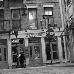
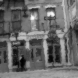
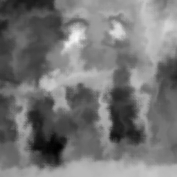
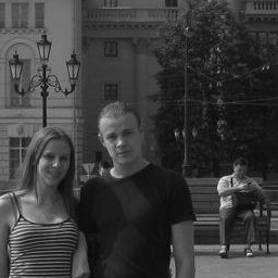
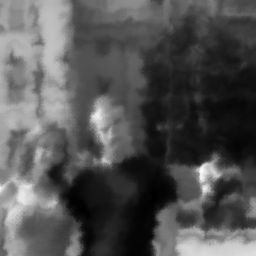
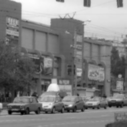
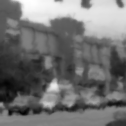
Figure 1: Examples of available sequences in the SOTIS dataset. The used ground-truth images are given in the left column. The corresponding weak and strong turbulence scenarios are illustrated in the center and right columns, respectively.

2.2 Evaluation protocol

Given the large literature on atmospheric turbulence mitigation, it becomes imperative to define some evaluation protocol to fairly and quantitatively compare the different algorithms. Algorithm evaluation has been considered in 18, 68, 13, 4, 69, 70. However, these articles do not really define a specific protocol, and mostly struggle of achieving their goal because of the lack of ground-truth images in most cases.
Since SOTIS provides the ground-truths images (which will be denoted $f_{gt}$ hereafter), we propose to use the widely accepted peak signal to noise ratio (PSNR) and structural similarity index measure (SSIM) metrics respectively defined by (we denote $f_{rest}$ the restored image):

$$PSNR(f_{gt},f_{rest})=10\log_{10}\left(\frac{\max_{im}}{\|f_{gt}-f_{rest}\|_{2}^{2}}\right),$$

where $\max_{im}$ is the maximum value an image can reach (255 for 8-bits encoded images); and

$$SSIM(f_{gt},f_{rest})=\frac{(2\mu_{gt}\mu_{rest}+c_{1})(2\sigma_{gt,rest}+c_{2})}{(\mu_{gt}^{2}+\mu_{rest}^{2}+c_{1})(\sigma_{gt}^{2}+\sigma_{rest}^{2}+c_{2})},$$

where $\mu_{gt}$ and $\mu_{rest}$ are respectively the average of $f_{gt}$ and $f_{rest}$; $\sigma_{gt},\sigma_{rest},\sigma_{gt,rest}$ their variances and covariance, $c_{1},c_{2}$ two constants defined from the images dynamic range. Notice that the SSIM metric provides values in the range $[0,1]$ (1 being the best performance).
With the SOTIS dataset, we provide several MATLAB scripts where the user can easily plug any stabilization, deblurring or combined algorithms and create the appropriate directory structure to store his results. We also provide a script that parses all the results and build a CSV file that contains the corresponding PSNR and SSIM values. Any statistical software like R can then extract all the useful evaluation statistics (we also provide the R script we wrote to generate the results in this article).

3 Deep learning and turbulence mitigation

Neural networks have gained a lot attention towards recovering images degraded by blur caused by camera shake. These networks use a variety of techniques (we refer the reader to the review paper 77), and particularly show significant success in dynamic scene deblurring; which incorporates blur caused by moving objects in addition to the blur due to camera shake. Such architecture inverts the effect of a blur kernel that is non-uniform, i.e. it varies from pixel to pixel. Because atmospheric turbulence induced blur can be seen as such anisoplanatic blur, we evaluate the three best ranked architectures from 77 on the SOTIS dataset. Furthermore, we chose two other models that were not mentioned in 77, in order to analyze different neural networks architectures. Most neural networks for deblurring are designed to process single images, therefore we use the stabilization results as our input for these neural networks. We also try end-to-end training on a neural network that aims to achieve video deblurring and takes an entire sequence of images as input, thereby forgoing the need of the stabilization step. We consider the following networks for evaluation,

• Scale-recurrent Network for Deep Image Deblurring (SRN) 78

• Deep Multi-scale Convolutional Neural Network for Dynamic Scene Deblurring (DSD) 79

• DeblurGAN-v2 (DGv2) 80

• Deblurring using Analysis-Synthesis Networks Pair (ASD) 81

• Cascaded Deep Video Deblurring Using Temporal Sharpness Prior (CDVD-TSP) 82

It is common for such neural networks to use a U-Net based architecture 83 along with residual layers. Increasing the receptive field plays a key role and has been emphasized by DSD, SRN and CDVD-TSP. However, each neural network has a different method of increasing the receptive field. Apart from the multi-scale information that is extracted by the U-Net, an extra multi-scale pyramid decomposition is used in SRN by applying a U-Net at each resolution of the image. Then, the corresponding loss function is able to take into account the reconstruction at each specific resolution. The DSD architecture builds an IIR (Infinite Impulse Response) filter, while CDVD-TSP learns a temporal sharpness prior that is able to take into account long range dependency among the input sequence. Networks used for object detection and image segmentation, such as VGG16 84, have shown to be useful for deblurring since they can identify regions of uniform blur. Such strategy is used in DGv2 and DSD to better estimate the blur kernel. The DSD and ASD networks have a separate kernel estimation module, whereas other networks do not separate the process of kernel estimation and image deblurring. The networks ASD and DGv2 introduced the use of novel concepts such as cross correlation layers, and adapting relativistic warping to the LS GAN 80 loss.

4 Experimental evaluations

In this section, we present some evaluation results for both classic (i.e non-deep learning) and deep-learning based mitigation algorithms. Every algorithms are based on an initial stabilization step followed by some deblurring.

4.1 Non-Deep Learning case

We test two main approaches for the stabilization: 1) a temporal average, 2) the Mao-Gilles 9 algorithm based on optical flow. For the later, we experiment the use of two different regularizations: $TV$ (total variation) or $NLTV$ (non-local total variation); and two variations of the optical flow: Lucas-Kanade or $TVL^{1}$ (total variation + $L^{1}$). These different stabilization methods will be denoted, Temporal_Average, $TV-LK,TV-TVL1,NLTV-LK$ and $NLTV-TVL1$, respectively.
The used deblurring techniques are BATUD 47, CLS (framelet based deconvolution) 85, and ZWZ ($\ell^{2}-\ell_{p}$ sparse prior based variational model) 86.
We also test the wavelet fusion based algorithm proposed by 23, denoted ATM, and the lucky imaging approach developed in 35, denoted IRAT. These algorithms are combined approaches, i.e they have their own stabilization and deconvolution approaches.
The evaluation results are given in Figure 2. Figure 2(a) provides the overall results, i.e averaged over all stabilization algorithms. If clearly the CLS algorithm does not perform well compared with the others, we can see that all other methods perform quite equivalently. It is interesting to notice that the SSIM metric always remains below 0.6, i.e. there is room to improve the existing algorithms. Figure 2(b) shows the influence of the distance between the target and the sensor. As expected, the further the target (hence the worse the degradation), the lower the performances. Figure 2(c) illustrates the impact of the chosen stabilization algorithm. Surprisingly, the simple temporal averaging performs as good as more advanced stabilization algorithms. This tends to confirm the idea, that a simple mean transforms the degradation in an isotropic blur that can be managed by efficient standard deconvolution algorithms. Finally, Figures 2(d) and 2(e) give the performances with respect to the turbulence strength ($C_{n}^{2}$). Here again, as expected, the stronger the turbulence, the worse the degradation, and the lower the performances.

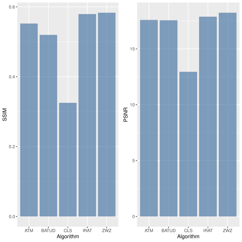
(a) Overall performances (averaged across all stabilization algorithms).

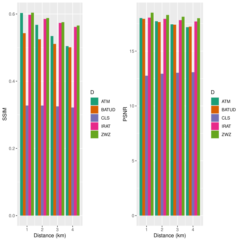
(b) Performance with respect to the sensor-target distance $L$.

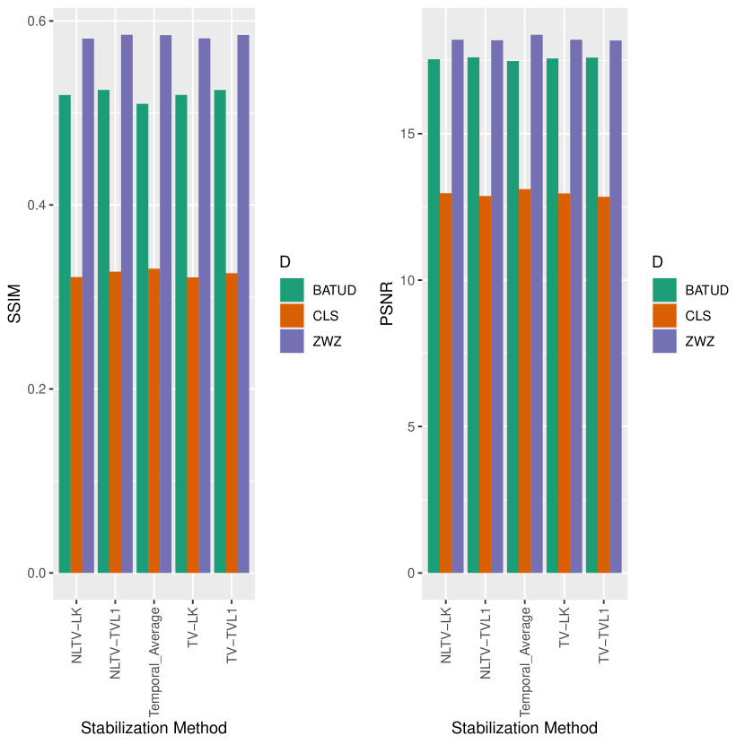
(c) Performance with respect stabilization.

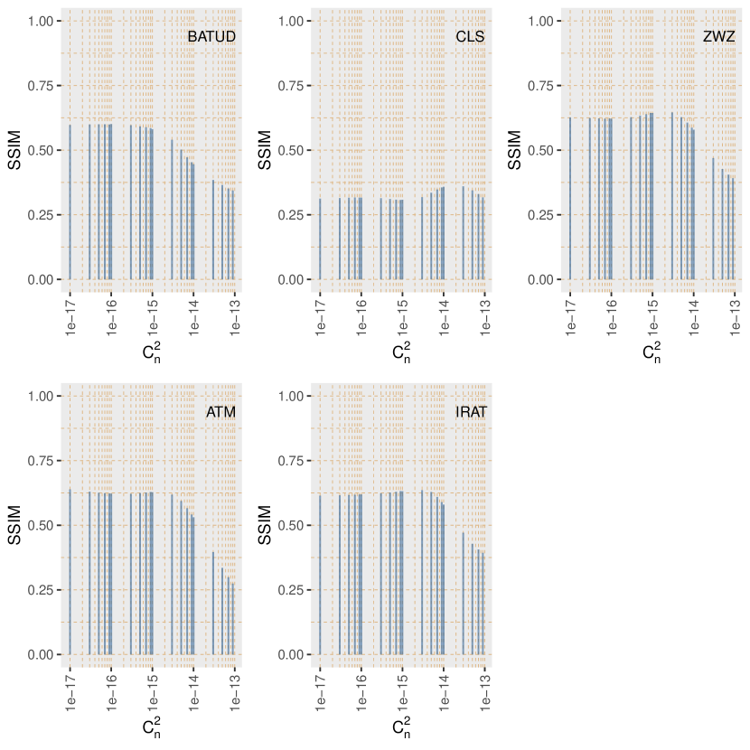
(d) Performance (SSIM) with respect to turbulence strength ($C_{n}^{2}$).

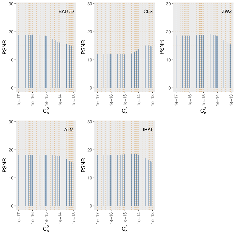
(e) Performance (PSNR) with respect to turbulence strength ($C_{n}^{2}$).

Figure 2: Performances results for Non-Deep Learning algorithms.

4.2 Deep learning case

We evaluate the performance of the five selected neural network models mentioned in Section 3 on the SOTIS dataset. Unlike the more popular GoPro dataset that was created by averaging a sequence of frames and geared towards simulating motion-blur, the SOTIS dataset contains images that are simulated using real physics and is geared towards providing realistic atmospheric turbulence scenarios. Thus by using the SOTIS dataset, we wish to observe how well the networks adapt to mitigating atmospheric turbulence, instead of removing blur caused by camera shake as originally intended. Because the SOTIS dataset contains a larger number of samples, we perform less epochs for training compared to the original papers. Note that, due to a lack of time, we only ran the evaluations on the $NLTV-LK$ and $NLTV-TVL1$ stabilized sequences. The number of iterations performed by the authors are indicated in Table 1 and the number of iterations we performed are indicated in Table 2 (using $NLTV-LK$), Table 3 (using $NLTV-TVL1$) and Table 4. Except for the number of epochs, we used default settings for all models as provided by their respective authors. Another difference compared to the original papers is the number of channels used for the input images to the networks. The networks used RGB images for their training, however since SOTIS only contains grayscale images, we converted the grayscale images to RGB images by copying the same values across all three channels. However, we noticed that such conversion caused convergence problems for ASD using $NLTV-LK$. To circumvent this issue, we stopped the algorithm one step before we detected a sign of divergence.
We first evaluate the testing set on the pre-trained networks provided by their respective authors. Because the SOTIS dataset is significantly different from the GoPro dataset, we re-train all networks using SOTIS and present how well re-training compares against the pre-trained network parameters. Using pre-trained parameters would make sense if we expect the probability distribution of the blur kernel for motion deblurring to be comparable to the blur kernel causing atmospheric turbulence. Comparing the results from Figure 4 and Figure 3, we observe that re-training significantly improves the quality of the estimated image.

Second, we split the SOTIS dataset for training and testing in a 75:25 ratio. We use the sequence of blury frames to train CDVD-TSP, while we feed the stabilized images to all other deblurring networks.

Table 1: Parameters Used for Pre-Training Evaluation

Method	Batch Size	Steps	Epochs	Training Examples	Total
DSD	20	200000	1887	2103	4000000
DGv2	5	600000	300	10000	3000000
ASD	4	1100000	105	42000	4400000
SRN	16	264000	2000	2103	4206000
CDVD-TSP	8	381500	500	6100	3050000

Table 2: Parameters Used for Re-Training Evaluation NLTV-LK

Method	Batch Size	Steps	Epochs	Training Examples	Total
DSD	14	200000	217	12900	2800000
DGv2	5	288960	112	12900	1444800
ASD	6	120400	56	12900	722400
SRN	10	983000	763	12900	9830000

Table 3: Parameters Used for Re-Training Evaluation NLTV-TVL1

Method	Batch Size	Steps	Epochs	Training Examples	Total
DSD	14	187500	204	12900	2625000
DGv2	5	774000	300	12900	3870000
ASD	6	290250	135	12900	1741500
SRN	10	1022000	793	12900	10220000

Table 4: Parameters Used for Re-Training Evaluation CDVD-TSP

Method	Batch Size	Steps	Epochs	Training Examples	Total
CDVD-TSP	1	4515000	7	645000	4515000

The performances of each algorithms are very different from each other for re-training. Looking at the overall performance in Figure 3(a), we see that ASD performed much better than the rest of the algorithms. We notice that DGv2 performs better than SRN, whereas the results in  77 suggested that SRN performed better at mitigating motion blur. This seems to indicate that the task of atmospheric turbulence mitigation is indeed different from removing a camera shake induced blur. The overall performance of all re-trained networks shows better results than non-deep learning algorithms. This recommends that investigating the use of neural networks for atmospheric turbulence mitigation could lead to better algorithms than the current state of the art.
The difference in the choice of stabilization method for pre-training is less significant as shown in Figure 4(c) compared to that for re-training in Figure 3(c). However, $NLTV-TVLK$ performs much better for SRN after retraining.
The performances of all networks decrease with respect to distance as indicated in Figure 3(b) (for re-training) and Figure 4(b) (for pre-training). A similar decline in performance can also be seen with respect to $C_{n}^{2}$ in Figures 3(d) and 3(e) (for re-training) and in Figures 4(d) and 4(e) (for pre-training).

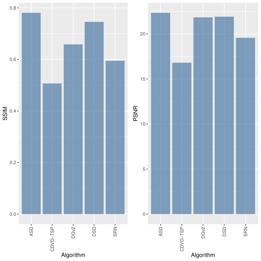
(a) Overall performances (averaged across all stabilization algorithms).

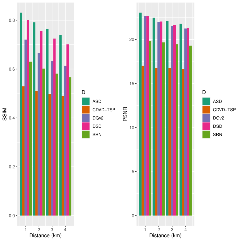
(b) Performance with respect to the sensor-target distance $L$.

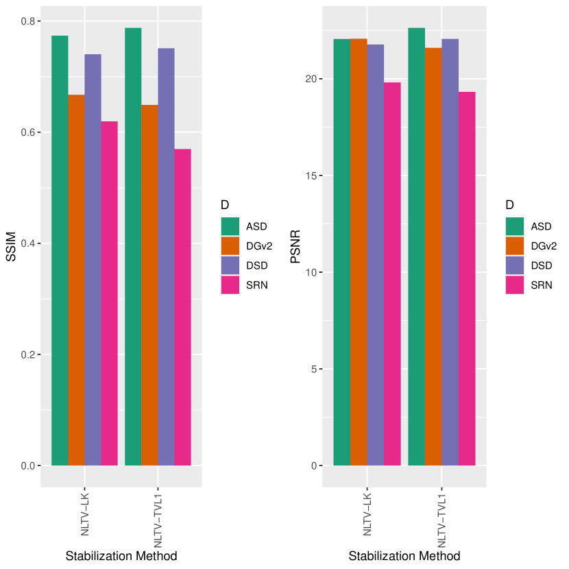
(c) Performance with respect to stabilization.

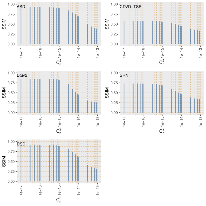
(d) Performance (SSIM) with respect to turbulence strength ($C_{n}^{2}$).

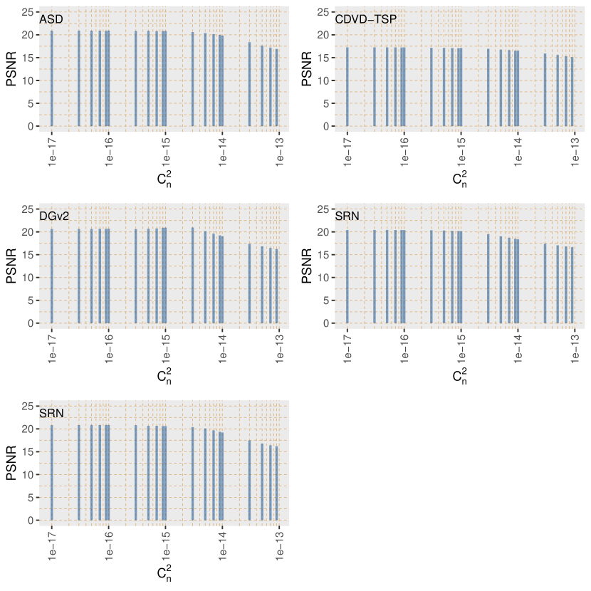
(e) Performance (PSNR) with respect to turbulence strength ($C_{n}^{2}$).

Figure 3: Performances results for Re-trained Deep Learning algorithms.

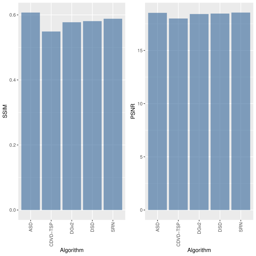
(a) Overall performances (averaged across all stabilization algorithms).

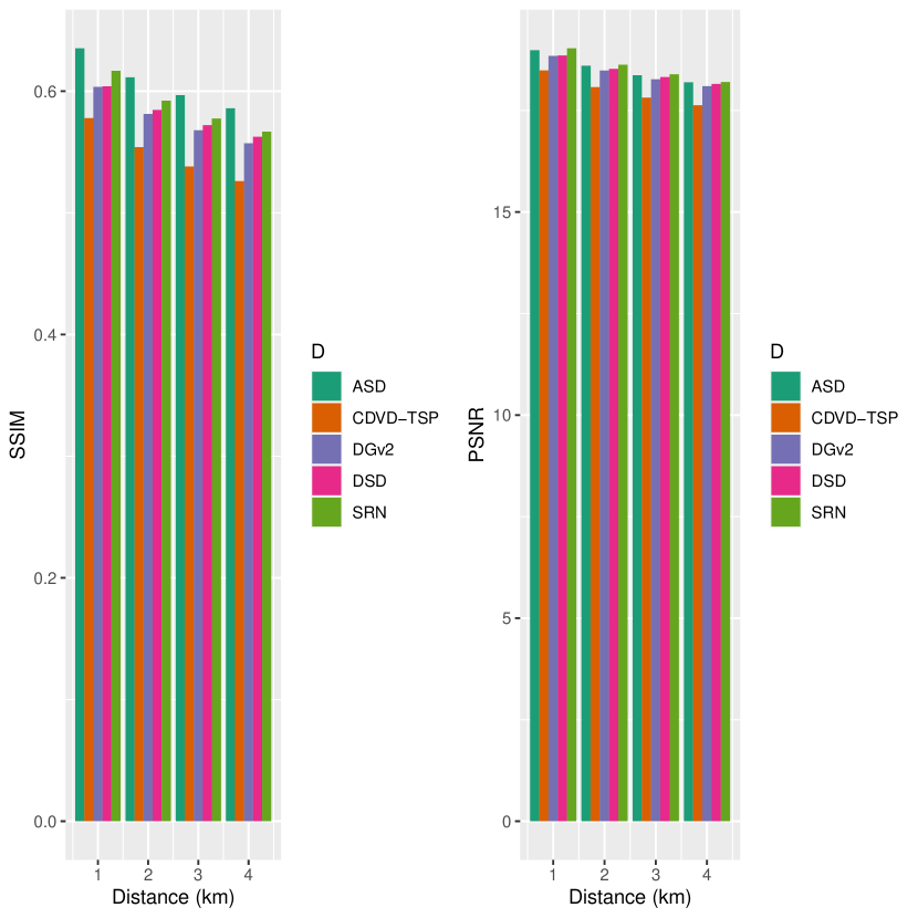
(b) Performance with respect to the sensor-target distance $L$.

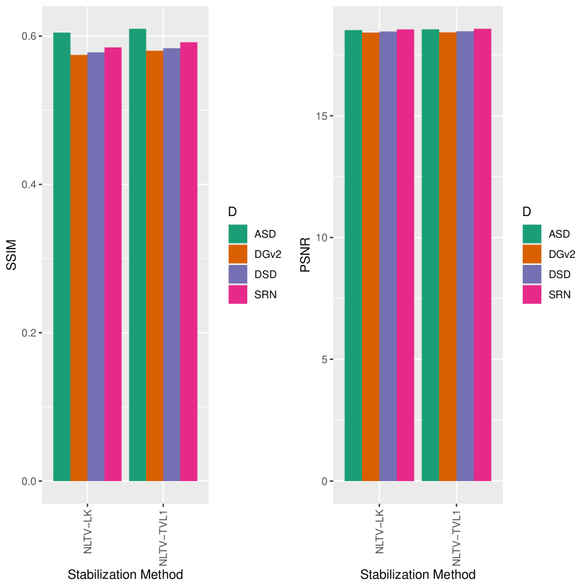
(c) Performance with respect to stabilization.

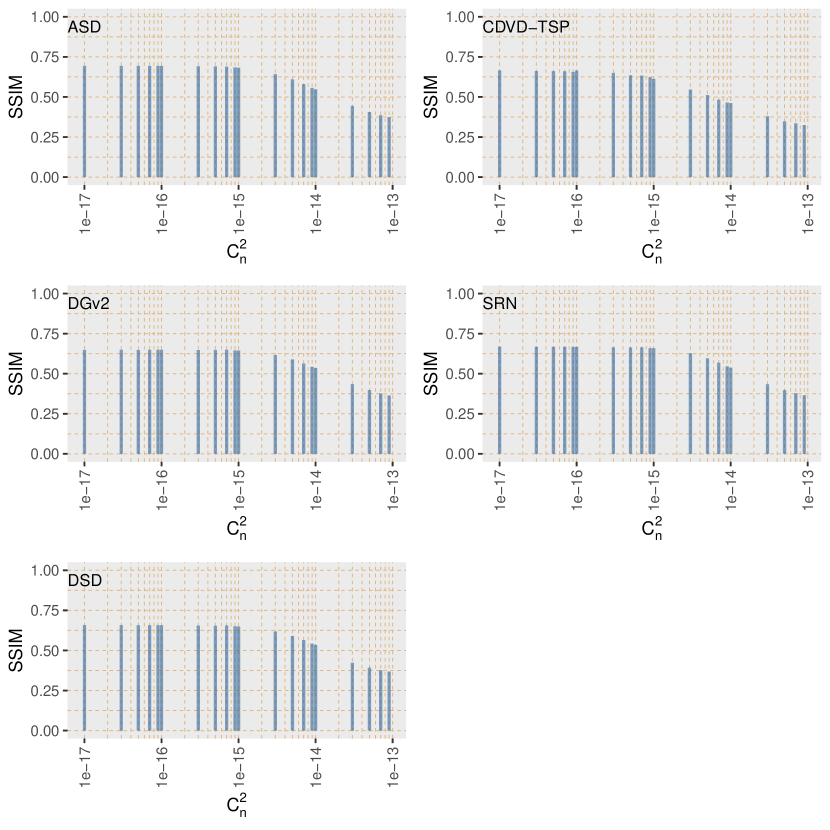
(d) Performance (SSIM) with respect to turbulence strength ($C_{n}^{2}$).

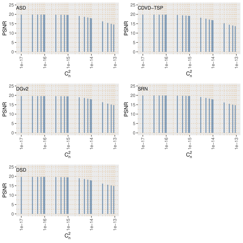
(e) Performance (PSNR) with respect to turbulence strength ($C_{n}^{2}$).

Figure 4: Performances results for Pre-trained Deep Learning algorithms.

The observed performances of CDVD-TSP indicate that either a separate stabilization stage is needed, or specific neural networks based stabilization architectures must be developed. For instance, end-to-end training could be improved by potentially incorporating some of the traditional stabilization algorithms into the network. Although our experiments are able to tell how the networks compare against each other, experiments could be performed to study which aspect of the networks contribute to its deblurring power. That could involve removing aspects of the network and seeing how much the performance deteriorates. This could further be used to create networks that are more efficient to tackle atmospheric turbulence in images.

5 Conclusion

In this article, we have introduced a new publicly available large dataset, SOTIS, intended to provide simulated sequences impacted by different scenarios of atmospheric turbulence. It also provides the corresponding ground-truth images which can be used for both performing qualitative evaluations of mitigation algorithms, as well as to train neural network architectures for future research. We have presented a first set of evaluation results in both the non-deep learning and deep learning cases. We observe that such systematic evaluation permits to better understand the importance and role of each stage in the restoration process.
In future work, we expect to run many more algorithm evaluations to have a clear picture of today’s achievements. We also plan to use the learned knowledge to develop more specific deep learning based architectures.

- [1] Mugnier, L., Besnerais, G. L., and Meimon, S., [Bayesian Approach to Inverse Problems ], ch. 10 - Inversion in optical imaging through atmospheric turbulence, John Wiley (2008).
- [2] Schutte, K., van Eekeren, A. W. M., Dijk, J., Schwering, P. B. W., van Iersel, M., and Doelman, N. J., “An overview of turbulence compensation,” in [Electro-Optical Remote Sensing, Photonic Technologies, and Applications VI ], Kamerman, G. W., Steinvall, O., Bishop, G. J., Gonglewski, J., Gruneisen, M. T., Dusek, M., Rarity, J. G., Lewis, K. L., Hollins, R. C., and Merlet, T. J., eds., 8542, 212 – 221, International Society for Optics and Photonics, SPIE (2012).
- [3] Yao, L., Shang, Y., and Fu, D., “Influence of atmospheric turbulence on optical measurement: a case report and review of literature,” in [Selected Papers of the Photoelectronic Technology Committee Conferences held November 2015 ], Bao, W. and Lv, Y., eds., 9796, 14 – 21, International Society for Optics and Photonics, SPIE (2016).
- [4] Huebner, C. S., “Local motion compensation in image sequences degraded by atmospheric turbulence: a comparative analysis of optical flow vs. block matching methods,” in [Optics in Atmospheric Propagation and Adaptive Systems XIX ], Stein, K. U. and Gonglewski, J. D., eds., 10002, 122 – 132, International Society for Optics and Photonics, SPIE (2016).
- [5] Fraser, D., Lambert, A., Jahromi, M. R. S., Tahtali, M., and Clyde, D., “Anisoplanatic image restoration at adfa,” in [Proc. VIIth Digital Image Computing: Techniques and Applications ], C., S., H., T., S., O., and T., A., eds., 19–28 (2003).
- [6] Gepshtein, S., Shtainman, A., and Fishbain, B., “Restoration of atmospheric turbulent video containing real motion using rank filtering and elastic image registration,” in [Proceedings of EUSIPCO ], (September 2004).
- [7] Zamek, S. and Yitzhaky, Y., “Turbulence strength estimation and super-resolution from an arbitrary set of atmospherically degraded images,” in [Atmospheric Optical Modeling, Measurement, and Simulation II ], Hammel, S. M. and Kohnle, A., eds., 6303, 27 – 37, International Society for Optics and Photonics, SPIE (2006).
- [8] Shimizu, M., Yoshimura, S., Tanaka, M., and Okutomi, M., “Super-resolution from image sequence under influence of hot-air optical turbulence,” in [IEEE Conference on Computer Vision and Pattern Recognition, 2008 (CVPR 2008) ], 1–8 (23-28 June 2008).
- [9] Mao, Y. and Gilles, J., “Non rigid geometric distortions correction - application to atmospheric turbulence stabilization,” Journal of Inverse Problems and Imaging 6(3), 531–546 (2012).
- [10] van Eekeren, A. W. M., Kruithof, M. C., Schutte, K., Dijk, J., van Iersel, M., and Schwering, P. B. W., “Patch-based local turbulence compensation in anisoplanatic conditions,” in [Infrared Imaging Systems: Design, Analysis, Modeling, and Testing XXIII ], Holst, G. C. and Krapels, K. A., eds., 8355, 263 – 270, International Society for Optics and Photonics, SPIE (2012).
- [11] Yang, B., Zhang, W., Xie, Y., and Li, Q., “Distorted image restoration via non-rigid registration and lucky-region fusion approach,” in [Proceedings of the Third International Conference on Information Science and Technology ], 414–418 (March 23-25 2013).
- [12] Gilles, J., “Mao-Gilles stabilization algorithm,” Image Processing On Line 2013, 173–182 (July 2013).
- [13] Gal, R., Kiryati, N., and Sochen, N., “Progress in the restoration of image sequences degraded by atmospheric turbulence,” Pattern Recognition Letters 48, 8–14 (October 2014).
- [14] Song, C., Ma, K., Li, A., Chen, X., and Xu, X., “Diffraction-limited image reconstruction with SURE for atmospheric turbulence removal,” Infrared Physics & Technology 71, 171–174 (2015).
- [15] Xie, Y., Zhang, W., Tao, D., Hu, W., Qu, Y., and Wang, H., “Removing turbulence effect via hybrid total variation and deformation-guided kernel regression,” IEEE Transaction on Image Processing 25(10), 4943–4958 (2016).
- [16] Nieuwenhuizen, R. P. J., van Eekeren, A. W. M., Dijk, J., and Schutte, K., “Dynamic turbulence mitigation with large moving objects,” in [Electro-Optical and Infrared Systems: Technology and Applications XIV ], Huckridge, D. A., Ebert, R., and Bürsing, H., eds., 10433, 196 – 207, International Society for Optics and Photonics, SPIE (2017).
- [17] Nieuwenhuizen, R. and Schutte, K., “Deep learning for software-based turbulence mitigation in long-range imaging,” in [Artificial Intelligence and Machine Learning in Defense Applications ], Dijk, J., ed., 11169, 153–162, International Society for Optics and Photonics, SPIE (2019).
- [18] Huebner, C. S. and Greco, M., “Blind deconvolution algorithms for the restoration of atmospherically degraded imagery: a comparative analysis,” in [Optics in Atmospheric Propagation and Adaptive Systems XI ], Kohnle, A., Stein, K., and Gonglewski, J. D., eds., 7108, 166 – 177, International Society for Optics and Photonics, SPIE (2008).
- [19] Huebner, C. S., “Compensating image degradation due to atmospheric turbulence in anisoplanatic conditions,” in [Mobile Multimedia/Image Processing, Security, and Applications 2009 ], Agaian, S. S. and Jassim, S. A., eds., 7351, 43 – 53, International Society for Optics and Photonics, SPIE (2009).
- [20] Huebner, C. S. and Scheifling, C., “Software-based mitigation of image degradation due to atmospheric turbulence,” in [Optics in Atmospheric Propagation and Adaptive Systems XIII ], Stein, K. and Gonglewski, J. D., eds., 7828, 198 – 209, International Society for Optics and Photonics, SPIE (2010).
- [21] Halder, K. K., Tahtali, M., and Anavatti, S. G., “High precision restoration method for non-uniformly warped images,” in [Advanced Concepts for Intelligent Vision Systems - 15th International Conference, ACIVS, Proceedings ], Lecture Notes in Computer Science 8192, 60–67, Springer, Poznan, Poland (October 28-31 2013).
- [22] Halder, K., Tahtali, M., and Anavatti, S., “A fast restoration method for atmospheric turbulence degraded images using non-rigid image registration,” in [2013 International Conference on Advances in Computing, Communications and Informatics (ICACCI) ], 394–399 (2013).
- [23] Anantrasirichai, N., Achim, A., Kingsbury, N. G., and Bull, D. R., “Atmospheric turbulence mitigation using complex wavelet-based fusion,” IEEE Transaction in Image Processing 22, 2398–2408 (June 2013).
- [24] Frakes, D. H., Monaco, J. W., and Smith, M. J. T., “Suppression of atmospheric turbulence in video using an adaptive control grid interpolation approach,” Proceedings of the IEEE International Conference on Acoustics, Speech, and Signal Processing. 3, 1881–1884 (2001).
- [25] Zhu, X. and Milanfar, P., “Image reconstruction from videos distorted by atmospheric turbulence,” in [Visual Information Processing and Communication ], Said, A. and Guleryuz, O. G., eds., 7543, 228 – 235, International Society for Optics and Photonics, SPIE (2010).
- [26] Zwart, C. M., Pracht, R. J., and Frakes, D. H., “Improved motion estimation for restoring turbulence distorted video,” in [Proceedings of SPIE ], Infrared Imaging Systems: Design, Analysis, Modeling, and Testing XXIII 8355, 83550E–1–83550E–9 (2012).
- [27] He, R., Wang, Z., Fan, Y., and Fengg, D., “Atmospheric turbulence mitigation based on turbulence extraction,” in [2016 IEEE International Conference on Acoustics, Speech and Signal Processing (ICASSP) ], 1442–1446 (March 2016).
- [28] Unser, M., Trus, B. L., and Eden, M., “Iterative restoration of noisy elastically distorted periodic images.,” Signal Processing 17, 191–200 (July 1989).
- [29] Zhu, X. and Milanfar, P., “Removing atmospheric turbulence via space-invariant deconvolution,” IEEE Transactions on Pattern Analysis and Machine Intelligence 35, 157–170 (January 2013).
- [30] Furhad, M. H., Tahtali, M., and Lambert, A., “Restoring atmospheric-turbulence-degraded images,” Applied Optics 55, 5082–5090 (July 2016).
- [31] Gilles, J., Dagobert, T., and Franchis, C. D., “Atmospheric turbulence restoration by diffeomorphic image registration and blind deconvolution,” in [Advanced Concepts for Intelligent Vision Systems (ACIVS) ], (October 2008).
- [32] Micheli, M., Lou, Y., Soatto, S., and Bertozzi, A. L., “A linear systems approach to imaging through turbulence,” Journal of Mathematical Imaging and Vision 48(1), 185–201 (2013).
- [33] Aubailly, M., Vorontsov, M. A., Carhart, G. W., and Valley, M. T., “Automated video enhancement from a stream of atmospherically-distorted images: the lucky-region fusion approach,” in [Atmospheric Optics: Models, Measurements, and Target-in-the-Loop Propagation III ], Hammel, S. M., van Eijk, A. M. J., and Vorontsov, M. A., eds., 7463, 104 – 113, International Society for Optics and Photonics, SPIE (2009).
- [34] Lou, Y., Kang, S. H., Soatto, S., and Bertozzi, A. L., “Video stabilization of atmospheric turbulence distortion,” Inverse Problems and Imaging 7(3), 839–861 (2013).
- [35] Mao, Z., Chimitt, N., and Chan, S. H., “Image reconstruction of static and dynamic scenes through anisoplanatic turbulence,” IEEE Transactions on Computational Imaging 6, 1415–1428 (October 2020).
- [36] Micheli, M., “The centroid method for imaging through turbulence,” tech. rep., MAP5, Université Paris Descartes (June 2012).
- [37] Meinhardt-Llopis, E. and Micheli, M., “Implementation of the Centroid Method for the Correction of Turbulence,” Image Processing On Line 4, 187–195 (2014).
- [38] Sadot, D., Rosenfeld, A., Shuker, G., and Kopeika, N. S., “High-resolution restoration of images distorted by the atmosphere, based on an average atmospheric modulation transfer function,” Optical Engineering 34(6), 1799 – 1807 (1995).
- [39] Schulz, T. J., “Nonlinear models and methods for space-object imaging through atmospheric turbulence,” in [IEEE Workshop on Nonlinear Signal and Image Processing ], 1(423) (1997).
- [40] Bondeau, C. and Bourennane, E.-B., “Comparison of classical and multiscale spatially adaptive filters for the restoration of images degraded by atmospheric turbulence,” in [Applications of Digital Image Processing XXI ], Tescher, A. G., ed., 3460, 761 – 766, International Society for Optics and Photonics, SPIE (1998).
- [41] Xu, J.-Y. and Wang, Y.-J., “Deconvolution method of atmospheric spectra and its application in atmospheric remote sensing,” in [Proc. SPIE 3501, Optical Remote Sensing of the Atmosphere and Clouds ], 390–400 (1998).
- [42] Cochran, W., Plemmons, R., and Torgersen, T., “Algorithms and software for atmospheric image reconstruction,” in [Proceedings of the AMOS Technical Conference ], (1999).
- [43] Li, D., Mersereau, R. M., Frakes, D. H., and Smith, M. J. T., “A new method for suppressing optical turbulence in video,” in [2005 13th European Signal Processing Conference ], 1–4 (2005).
- [44] van Iersel, M. and van Eijk, A. M. J., “Estimating turbulence in images,” in [Free-Space Laser Communications X ], Majumdar, A. K. and Davis, C. C., eds., 7814, 197 – 206, International Society for Optics and Photonics, SPIE (2010).
- [45] Droege, D. R., Hardie, R. C., Allen, B. S., Dapore, A. J., and Blevins, J. C., “A real-time atmospheric turbulence mitigation and super-resolution solution for infrared imaging systems,” in [Infrared Imaging Systems: Design, Analysis, Modeling, and Testing XXIII ], Holst, G. C. and Krapels, K. A., eds., 8355, 234 – 250, International Society for Optics and Photonics, SPIE (2012).
- [46] Gilles, J. and Osher, S., “Fried deconvolution,” in [SPIE Defense, Security and Sensing conference ], (April 2012).
- [47] Deledalle, C.-A. and Gilles, J., “Blind Atmospheric TUrbulence Deconvolution,” IET Image Processing 14(14), 3422–3432 (2020).
- [48] Gao, X., Jiang, Z., He, X., Kong, Y., Wang, S., and Liu, C., “Iterative imaging through strong dynamic turbulence media,” Optics and Lasers in Engineering 149, 106779 (2022).
- [49] Lemaitre, M., Mériaudeau, F., Laligant, O., and Blanc-Talon, J., “Distant horizontal ground observation: atmospheric perturbation simulation and image restoration,” in [Conférence Signal Image Technologie and Internet Based Systems (SITIS) ], (2005).
- [50] Lemaitre, M., Mériaudeau, F., Laligant, O., and Blanc-Talon, J., “Evaluation of infrared image restoration techniques,” in [European SPIE Conference ], (2006).
- [51] Denker, C., Tritschler, A., and Löfdahl, M., [Encyclopedia of Optical Engineering ], ch. Image reconstruction, 1–19, Marcel Dekker Inc. (2004).
- [52] Li, D. and Simske, S., “Atmospheric turbulence degraded image restoration by kurtosis minimization,” IEEE Geoscience and Remote Sensing Letters 6(2), 244–247 (2009).
- [53] Li, D., Mersereau, R. M., and Simske, S., “Atmospheric turbulence-degraded image restoration using principal components analysis,” IEEE Geoscience and Remote Sensing Letters 4, 340–344 (July 2007).
- [54] Lu, Q., Zhuoma, S., Ge, B., and Tian, Q., “Turbulent-degraded image restoration via improved principal component analysis method,” Journal of Modern Optics 68(17) (2021).
- [55] Hong, H., Li, L., and Zhang, T., “Blind restoration of real turbulence-degraded image with complicated backgrounds using anisotropic regularization,” Optics Communications 285(24), 4977–4986 (2012).
- [56] Zuo, H., Zhang, Q., and Zhao, R., “An efficiency restoration method for turbulence-degraded image base on improved SeDDaRA method,” in [International Symposium on Photoelectronic Detection and Imaging 2009: Advances in Infrared Imaging and Applications ], Puschell, J., mei Gong, H., Cai, Y., Lu, J., and dong Fei, J., eds., 7383, 1090 – 1097, International Society for Optics and Photonics, SPIE (2009).
- [57] Huebner, C. S. and Gladysz, S., “Simulation of atmospheric turbulence for a qualitative evaluation of image restoration algorithms with motion detection,” in [Optics in Atmospheric Propagation and Adaptive Systems XV ], Stein, K. and Gonglewski, J., eds., 8535, 128 – 136, International Society for Optics and Photonics, SPIE (2012).
- [58] Holmes, R. and Gudimetla, V. S. R., “Image reconstructions with active illumination in strong-turbulence scenarios with single-frame blind deconvolution approaches,” Appl. Opt. 58, 7823–7835 (Oct 2019).
- [59] Gilles, J. and Osher, S., “Wavelet burst accumulation for turbulence mitigation,” Journal of Electronic Imaging 25(3), 033003–1–033003–9 (2016).
- [60] Hajmohammadi, S., Nooshabadi, S., Archer, G. E., and Bos, J. P., “Parallel hybrid bispectrum-multi-frame blind deconvolution image reconstruction technique,” Journal of Real-Time Image Processing 16(4) (2019).
- [61] Chunsheng, L., Hanyu, H., and Tianxu, Z., “Research on a novel restoration algorithm of turbulence-degraded images with alternant iterations,” Journal of Systems Engineering and Electronics 17(3), 477–482 (2006).
- [62] Harmeling, S., Sra, S., Hirsch, M., and Schölkopf, B., “Multiframe blind deconvolution, super-resolution, and saturation correction via incremental EM,” in [Proceedings of 2010 IEEE 17th International Conference on Image Processing ], 3313–3316 (September 2010).
- [63] Hirsch, M., Sra, S., Scholkopf, B., and Harmeling, S., “Efficient filter flow for space-variant multiframe blind deconvolution,” in [Computer Vision and Pattern Recognition Conference ], (2010).
- [64] liang Wang, L., wei Tao, Z., Li, M., and Gao, X., “Restoration algorithm of heavy turbulence degraded image for space target based on regularization,” in [International Symposium on Photoelectronic Detection and Imaging 2011: Space Exploration Technologies and Applications ], Zarnecki, J. C., Nardell, C. A., Shu, R., Yang, J., and Zhang, Y., eds., 8196, 214 – 221, International Society for Optics and Photonics, SPIE (2011).
- [65] Duan, L., Sun, S., Zhang, J., and Xu, Z., “Deblurring turbulent images via maximizing regularization,” Symmetry 13 (2021).
- [66] Bai, X., Liu, M., He, C., Dong, L., Zhao, Y., and Liu, X., “Restoration of turbulence-degraded images based on deep convolutional network,” in [Proceedings of SPIE Optical Engineering + Applications ], Michael E. Zelinski, Tarek M. Taha, J. H. A. A. S. A. K. M. I., ed., Applications of Machine Learning 11139 - 111390B, 111390B–1–111390B–9 (2019).
- [67] Espinola, R. L., Aghera, S., Thompson, R., and Miller, J., “Turbulence degradation and mitigation performance for handheld weapon ID,” in [Infrared Imaging Systems: Design, Analysis, Modeling, and Testing XXIII ], Holst, G. C. and Krapels, K. A., eds., 8355, 251 – 262, International Society for Optics and Photonics, SPIE (2012).
- [68] van Eekeren, A. W. M., Huebner, C. S., Dijk, J., Schutte, K., and Schwering, P. B. W., “Evaluation of turbulence mitigation methods,” in [Infrared Imaging Systems: Design, Analysis, Modeling, and Testing XXV ], Holst, G. C., Krapels, K. A., Ballard, G. H., Jr., J. A. B., and Jr., R. L. M., eds., 9071, 362 – 375, International Society for Optics and Photonics, SPIE (2014).
- [69] Kozacik, S., Paolini, A., Sherman, A., Bonnett, J., and Kelmelis, E., “Quantifying the improvement of turbulence mitigation technology,” in [Long-Range Imaging II ], Kelmelis, E. J., ed., 10204, 40 – 48, International Society for Optics and Photonics, SPIE (2017).
- [70] Yang, T. and Maraev, A. A., “Comparison of restoration methods for turbulence-degraded images,” in [Optoelectronic Imaging and Multimedia Technology V ], Dai, Q. and Shimura, T., eds., 10817, 302 – 309, International Society for Optics and Photonics, SPIE (2018).
- [71] Pigois, L., Simulation de turbulence en imagerie flash laser, Master’s thesis, Université de Cergy-Pontoise (2004).
- [72] Thomas, S., “A simple turbulence simulator for adaptive optics,” in [Advancements in Adaptive Optics ], Calia, D. B., Ellerbroek, B. L., and Ragazzoni, R., eds., 5490, 766 – 773, International Society for Optics and Photonics, SPIE (2004).
- [73] Repasi, E. and Weiss, R., “Computer simulation of image degradations by atmospheric turbulence for horizontal views,” in [Infrared Imaging Systems: Design, Analysis, Modeling, and Testing XXII ], Holst, G. C. and Krapels, K. A., eds., 8014, 279 – 287, International Society for Optics and Photonics, SPIE (2011).
- [74] Rampy, R., Gavel, D., Dillon, D., and Thomas, S., “Production of phase screens for simulation of atmospheric turbulence,” Applied Optics 51, 8769–8778 (Dec 2012).
- [75] Chimitt, N. and Chan, S. H., “Simulating anisoplanatic turbulence by sampling correlated zernike coefficients,” in [2020 IEEE International Conference on Computational Photography (ICCP) ], 1–12 (24-26 April 2020).
- [76] Tretiak, E., Barinova, O., Kohli, P., and Lempitsky, V., “Geometric image parsing in man-made environments,” International Journal of Computer Vision 97, 305–321 (2012).
- [77] Koh, J., Lee, J., and Yoon, S., “Single-image deblurring with neural networks: A comparative survey,” Computer Vision and Image Understanding 203, 103134 (2021).
- [78] Tao, X., Gao, H., Wang, Y., Shen, X., Wang, J., and Jia, J., “Scale-recurrent network for deep image deblurring,” CoRR abs/1802.01770 (2018).
- [79] Nah, S., Kim, T. H., and Lee, K. M., “Deep multi-scale convolutional neural network for dynamic scene deblurring,” CoRR abs/1612.02177 (2016).
- [80] Kupyn, O., Martyniuk, T., Wu, J., and Wang, Z., “Deblurgan-v2: Deblurring (orders-of-magnitude) faster and better,” CoRR abs/1908.03826 (2019).
- [81] Kaufman, A. and Fattal, R., “Deblurring using analysis-synthesis networks pair,” CoRR abs/2004.02956 (2020).
- [82] Pan, J., Bai, H., and Tang, J., “Cascaded deep video deblurring using temporal sharpness prior,” CoRR abs/2004.02501 (2020).
- [83] Ronneberger, O., Fischer, P., and Brox, T., “U-net: Convolutional networks for biomedical image segmentation,” CoRR abs/1505.04597 (2015).
- [84] Simonyan, K. and Zisserman, A., “Very deep convolutional networks for large-scale image recognition,” (2015).
- [85] Cai, J.-F., Ji, H., Liu, C., and Shen, Z., “Framelet-based blind motion deblurring from a single image,” IEEE Transactions on Image Processing 21, 562–572 (February 2012).
- [86] Zhang, H., Wipf, D., and Zhang, Y., “Multi-image blind deblurring using a coupled adaptive sparse prior,” in [2013 IEEE Conference on Computer Vision and Pattern Recognition ], IEEE, Portland, OR, USA (June 2013).