Mode sensitivity: Connecting Lagrangian coherent structures with modal analysis for fluid flows

Abstract

We consider the relationship between modal representations obtained from data-driven decomposition methods and Lagrangian Coherent Structures (LCSs). Mode sensitivity is used to describe this analysis as an extension of the model sensitivity framework developed by Kaszás and Haller [2020]. The method, based on the computation of the finite-time-Lyapunov exponent, uses modes from fluid data to compute the amplitude perturbations experienced by fluid particle trajectories along with their sensitivity to initial conditions. Demonstrations of the method are presented with both periodic and turbulent flows, including a kinematic flow model, experimental data from the wake past an oscillating foil, numerical data of the classical cylinder wake flow, and a direct numerical simulation (DNS) of a turbulent channel flow. Mode sensitivity fields reveal both quantitatively and qualitatively how the finite-time Lyapunov exponent fields used to visualize LCSs change due to the influence of modes or external perturbations.

Keywords — Lagrangian coherent structures, chaos, low-dimensional models

1 Introduction

Fluid flow is often characterized by the presence of complex processes such as instabilities, turbulent mixing, and vortex interactions. When many of these features are present, it is often useful to interpret and visualize fluid flows in terms of dominant patterns or coherent structures. Two of the leading representations used for understanding coherent structures are modal decompositions and Lagrangian Coherent Structure (LCS) analyses.

Modal decomposition methods have advanced over the past decade in finding reduced-complexity models from fluid flow data. These approaches can capture the coherent structures of interest in the form of modes. In practice, one may visualize contributions from individual modes (or small subsets of modes) to better understand the dominant features of the flow field. Techniques such as proper orthogonal decomposition (POD) and dynamic mode decomposition (DMD) used to identify energetically or dynamically important modes that can be linearly superposed to reconstruct the flow field [Taira et al., 2017]. The linear properties of this approximation are attractive from a mathematical point of view, and for interpreting modes as an additive component of the full flow field. These algorithms, as well as extensions such as spectral POD, balanced POD, and many variants of DMD, have been used successfully to identify flow patterns such as vortex shedding, vortex pairing and merging, Kelvin-Helmholtz instabilities, and very large scale motions (VLSMs) in turbulent flows [Taira et al., 2020, Saxton-Fox et al., 2022, Jones et al., 2024].

In practice, mode structures are extracted from Eulerian measurements of flow variables such as velocity, vorticity, or pressure. However, it has been argued that the identification of instantaneous flow features that are dynamically influential from such Eulerian analyses are generally frame-dependent and heuristic, which limits their reliability [Green et al., 2007, Haller, 2015]. Moreover, these representations often require a user-defined threshold for visualization, which can lead to difficulties in analyses such as vortex identification. Despite the limitations, modal analysis techniques have enabled significant progress towards the development of computationally efficient control-oriented models [Brunton and Noack, 2015, Taira et al., 2020].

Fluid flow can alternatively be analyzed in terms of Lagrangian Coherent Structures (LCSs), which are flow patterns that characterize fluid particle motion and transport. A data-driven method for computing LCSs is with the Finite-Time Lyapunov Exponent (FTLE) as described by Shadden et al. [2005], Haller [2015]. FTLEs characterize regions of maximum strain in the flow with respect to particle initial conditions. Thus an FTLE field can be interpreted as stable and unstable manifolds for particle trajectories. For fluid flows, the FTLE field can be useful for characterizing mixing regions and identifying vortices in an objective frame [Green et al., 2011, 2007]. In a sense, LCSs are the hidden skeleton of fluid flow that dictate fluid particle motion and transport. However, unlike modal representations, LCS fields lack clear hierarchical structures, which makes them less amenable to reduced-complexity modeling.

Techniques that combine the benefits of modal decompositions and LCS analyses have the potential to significantly further our understanding of coherent structures in fluid flows. Although under-explored in the fluid mechanics community, there have been prior efforts involving such hybrid analyses. MacMillan and Ouellette [2022] for instance demonstrated a Lagrangian-based decomposition method using a graph Fourier transform approach, whereby the eigenvalues of the graph Laplacian corresponded to structures with specific spatial scales. Similarly, Xie et al. [2020], proposed a decomposition method using a Lagrangian inner product encompassing both Eulerian and FTLE data to build a reduced order model. Approaches such as these hold significant potential for revealing new coherent structures relevant to particle trajectories while also capturing multi-scale features embedded within the flow.

The aim of this paper is to extend these concepts by studying how certain modes obtained from Eulerian measurements relate to the LCS of the fluid flow. We use an extension of the model sensitivity framework developed by Kaszás and Haller [2020]. While the FTLE field characterizes the sensitivity of particle trajectories to initial conditions, the model sensitivity framework can be used to account for stochastic and deterministic perturbations to the dynamical system itself. In the context of modal decomposition, these perturbations could be interpreted as the impact of individual modes on particle trajectories, or the collective influence of any modes neglected in a reduced complexity model.

The following section provides a brief review of the model sensitivity framework developed by Kaszás and Haller [2020]. As an illustrative example, the framework is used to evaluate the influence of a cross-stream perturbation on the LCS fields for a simple kinematic double gyre model. Subsequent examples extend the model sensitivity framework to assess the link between modal representations and LCSs for experimental and numerical flow field data. This includes modes obtained from: oscillating foil experiments [Jones et al., 2024]; direct numerical simulation (DNS) of the canonical cylinder flow wake at low Reynolds number [$Re=100$, see e.g., Kutz et al., 2016, Taira et al., 2020]; and DNS data for a broadbanded turbulent channel flow from the Johns Hopkins Turbulence Database [Graham et al., 2016].

This extended analysis, results in a Mode Sensitivity (MS) field, where the flow structure is represented in a Lagrangian space relative to a baseline (unperturbed) FTLE field. In comparison to coherent structures obtained via FTLEs, the MS provides additional insight and indicate regions in the flow field where the sensitivity from fluid particles is affected by Eulerian modes. The complementary flow structure which we term in this paper as the Lagrangian response can, in some sense, be considered as an LCS "mode" that effects particle motion and transport and could therefore inform flow control. While the modal analysis algorithms used in this paper include POD, DMD and optimized DMD, we emphasize that this analysis can also be used to consider the influence of other techniques that yield modal representations of the flow field, including spectral POD (SPOD), balanced POD (bPOD), and operator-based methods such as resolvent analysis [Towne et al., 2018, Rowley and Dawson, 2017, Herrmann et al., 2021].

2 Model Sensitivity

This section provides a brief review of the model sensitivity framework developed by Kaszás and Haller [2020]. The framework generates an upper-bound estimate for the difference between an unperturbed trajectory and a perturbed trajectory subject to stochastic or coherent disturbances. Let us first consider the dynamical system for the unperturbed particle trajectory $\mathbf{x}^{0}(t)$:

$$\dot{\mathbf{x}}^{0}(t)=\mathbf{f}(\mathbf{x}^{0},t).$$ (1)

The resulting trajectory, or flow map is

$$\boldsymbol{\Phi}_{t_{0}}^{t}=\mathbf{x}_{0}+\int_{t_{0}}^{t}\mathbf{f}(\mathbf{x}^{0}(\tau),\tau)d\tau.\$$ (2)

where $\mathbf{x}_{0}$ is the initial condition at time $t_{0}$, $t$ is a time between $t\in[t_{0},t_{0}+T]$, and $T$ is an period of integration. Next, we consider a purely deterministic perturbation to the dynamics which yield a system:

$$\dot{\mathbf{x}}^{\epsilon}(t)=\mathbf{f}(\mathbf{x}^{\epsilon},t)+\epsilon\mathbf{g}(\mathbf{x}^{\epsilon},t;\epsilon),$$ (3)

where $\epsilon$ is a small scalar parameter such that:

$$0\leq\epsilon\ll 1.$$ (4)

In the context of the present paper, the baseline system $\mathbf{f}$ can be considered the reduced-order modal representation while the perturbation $\mathbf{g}$ represents the modes of interest.

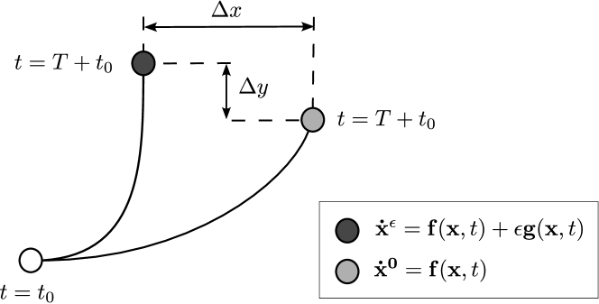
Figure 1: Illustration of perturbed (black) and unperturbed (gray) trajectories for a single fluid particle.

The aim is to find a closed form expression for the bounded error or trajectory uncertainty, $|\mathbf{x}^{\epsilon}(t)-\mathbf{x}^{0}(t)|$, as illustrated for a single fluid particle in figure 1. Assuming the flow map is smooth in $\epsilon$, we consider a Taylor series expansion about $\epsilon=0$ for the trajectory:

$$\mathbf{x}^{\epsilon}=\mathbf{x}^{0}+\epsilon\frac{\partial\mathbf{x}^{\epsilon}}{\partial\epsilon}\Bigg{|}_{\epsilon=0}+O(\epsilon^{2}),$$ (5)

where $\mathbf{x}^{0}$ is the trajectory solution for $\epsilon=0$, as in equation (2). For convenience, the partial derivative is rewritten as $\frac{\partial\mathbf{x}^{\epsilon}}{\partial\epsilon}=\boldsymbol{\eta}$. This also implies from equation (3) that:

$$\begin{split}\dot{\mathbf{x}}^{0}(t)+\epsilon\dot{\boldsymbol{\eta}}=\mathbf{f}(\mathbf{x}^{0},t)+\epsilon\boldsymbol{\eta}\nabla\mathbf{f}(\mathbf{x}^{0},t)+\epsilon\mathbf{g}(\mathbf{x}^{0},t)+O(\epsilon^{2}).\end{split}$$ (6)

The order $O$($\epsilon$) equation for the expansion of $x^{\epsilon}$ is therefore:

$$\dot{\boldsymbol{\eta}}=\nabla\mathbf{f}(\mathbf{x}^{0},t)\boldsymbol{\eta}+\mathbf{g}(\mathbf{x}^{0},t).$$ (7)

The above equation is an initial value problem (IVP) for $\boldsymbol{\eta}$ with the initial condition

$$\boldsymbol{\eta}(t_{0},\mathbf{x}_{0})=0,$$ (8)

and a homogeneous solution of the form

$$\boldsymbol{\eta}=\boldsymbol{\eta}_{0}e^{\int_{t_{0}}^{t}\nabla\mathbf{f}(\mathbf{x}^{0},s)ds}.$$ (9)

Following Kaszás and Haller [2020], the solution to the IVP of equation (7) can be expressed as

$$\boldsymbol{\eta}(t;t_{0},\mathbf{x}_{0})=\int_{t_{0}}^{t}\boldsymbol{D\Phi}_{s}^{t}\mathbf{g}(\mathbf{x}^{0}(s);0)ds,$$ (10)

where $\boldsymbol{D\Phi}_{s}^{t}$ is the flow map derivative of the unperturbed $\mathbf{f}(\mathbf{x}^{0},t)$ system. The term $\mathbf{g}(\mathbf{x}^{0}(s);0)$ represents the perturbation experienced by a fluid particle along the unperturbed trajectory $\boldsymbol{x^{0}}$ at time $s$.

2.1 Definition of Upper Bound

Early estimates of an upper bound for the trajectory uncertainty [see e.g., Kirchaber, 1976, Brauer, 1966] either required a priori knowledge of the perturbed trajectory or relied on Gronwall’s inequality [Guckenheimer and Holmes, 1983]. While Gronwall-type estimates yield a strict upper bound, they often overestimate the error, particularly for long term or spatially complex systems [Kaszás and Haller, 2020]. To estimate the leading order uncertainty in equation (10), a stronger upper limit can be identified using quantities that relate directly to the dynamics of the system. Choosing $t=t_{0}+T$, as our end interval, the solution can be bounded as

$$\begin{split}\epsilon|\boldsymbol{\eta}|\leq\epsilon\ \int_{t_{0}}^{t}|\boldsymbol{D\Phi_{s}^{t}}(\mathbf{x}^{0}(s))||\mathbf{g}(\mathbf{x}^{0}(s);0)ds|=\Delta_{\infty}\int_{t_{0}}^{t}\sqrt{\lambda_{s}^{t}(\mathbf{x}^{0}(s))}ds,\end{split}$$ (11)

where

$$\Delta_{\infty}=\epsilon\max\limits_{s\in[t_{0},\ t_{0}+T]}|\mathbf{g}(\mathbf{x}^{0}(s);0)|$$ (12)

is the maximum value of the perturbation field ($\epsilon\mathbf{g}$) along the unperturbed trajectory and $\lambda_{s}^{t}$ is the largest eigenvalue of the Cauchy-Stress Tensor $\boldsymbol{[D\Phi_{s}^{t}]^{*}D\Phi_{s}^{t}}$. Here, $[\cdot]^{*}$ is the conjugate transpose of $[\cdot]$.

Equation (11) is considered the universal error bound for the perturbed dynamical system shown in equation (3) relative to the unperturbed system from equation (1). It was shown by Kaszás and Haller [2020] that this error bound is a more rigorous estimate of the trajectory uncertainty in comparison to the Gronwall-type upper bound. Model Sensitivity (MS) is defined and related to the trajectory uncertainty as

$$(\epsilon|\mathbf{x}^{\epsilon}-\mathbf{x}^{0}|)^{2}\leq MS_{t_{0}}^{t}=\left(\Delta_{\infty}\int_{t_{0}}^{t}\sqrt{\lambda_{s}^{t}(\mathbf{x}^{0}(s))}ds\right)^{2}.$$ (13)

Thus, MS can be interpreted as the product of the amplitude uncertainty in the system, $\Delta_{\infty}$ caused by the perturbation $\epsilon\mathbf{g}(\mathbf{x}^{0},t)$, and the sensitivity with respect to initial conditions, which is characterized by the integral of the largest eigenvalue $\int_{t_{0}}^{t}\sqrt{\lambda_{s}^{t}(\mathbf{x}^{0}(s))}ds$.

2.2 Connection to the FTLE

The FTLE characterizes the material line elements in a flow over a finite time interval. To compute FTLE fields, particle motion is integrated over a time interval $T$ using standard techniques (e.g., the Runge-Kutta method). This process yields the flow map shown in equation (2). The forward FTLE is computed as:

$$\mathrm{FTLE}_{t_{0}}^{t}=\frac{1}{|T|}\log\sqrt{\lambda_{t_{0}}^{t}},$$ (14)

where $\lambda_{t_{0}}^{t}$ is the maximum eigenvalue of $[\boldsymbol{D\Phi}_{t_{0}}^{t}]^{*}\boldsymbol{D\Phi}_{t_{0}}^{t}$. When integrated forwards in time, the FTLE field reveals unstable or diverging manifolds of trajectories. Particles can also be integrated in backward time (from $t_{0}$ to $t$) to reveal stable or converging manifolds. This yields the backward FTLE:

$$\mathrm{FTLE}_{t}^{t_{0}}=\frac{1}{|T|}\log\sqrt{\lambda_{t}^{t_{0}}}.$$ (15)

Model Sensitivity (MS) for a perturbed dynamical system, as shown in equation (13), has a particular relationship to the forward FTLE for the baseline (unperturbed) system. Specifically, Kaszás and Haller [2020] show that:

$$\frac{\log\mathrm{MS}_{t_{0}}^{t}}{2|T|}=\mathrm{FTLE}_{t_{0}}^{t}+\zeta_{t_{0}}^{t},$$ (16)

where

$$\zeta_{t_{0}}^{t}=\frac{1}{|T|}\log\left(\Delta_{\infty}\int_{t_{0}}^{t}{\sqrt{\frac{\lambda_{s}^{t}}{\lambda_{t_{0}}^{t}}}}ds\right).$$ (17)

Thus, $\mathrm{MS}_{t_{0}}^{t}$ is the summation of two different effects: the sensitivity of the unperturbed system, as quantified by $\mathrm{FTLE}_{t_{0}}^{t}$, and the impact of disturbances along the unperturbed trajectory, which is characterized by $\zeta_{t_{0}}^{t}$. Since $\mathrm{MS}_{t_{0}}^{t}$ represents an upper bound on the trajectory uncertainty, the contribution from $\zeta_{t_{0}}^{t}$ can be interpreted as a potential perturbation to the FTLE field. In other words, $\mathrm{MS}_{t_{0}}^{t}$ and $\zeta_{t_{0}}^{t}$ provide complementary insights into system sensitivity, with the latter isolating the influence of the perturbation field. Note that equation (16) also holds for the backward FTLE field if the MS field in equation (13) is computed in backward time as $\mathrm{MS}_{t}^{t_{0}}$.

2.3 Example 1: Sensitivity for a model kinematic system

We now demonstrate the MS framework for a simple kinematic system. The model is first constructed using the double gyre flow field, which is an idealized two-dimensional model for large-scale ocean circulations and adheres to the continuity equation. The velocity field for the double gyre flow is expressed as:

$$\begin{split}\mathbf{u}(\mathbf{x},t)=\left[\begin{matrix}-\pi A\sin(\pi h(x,t))\cos(\pi y)\\ \pi A\cos(\pi h(x,t))\sin(\pi y)\end{matrix}\right],\end{split}$$ (18)

where $h(x,t)$ is a time dependent variable

$$h(x,t)=a(t)x^{2}+b(t)x,$$ (19)

containing the coefficients:

$$a(t)=\gamma\sin(\omega_{f}t),\ \ b(t)=1-2\gamma\sin(\omega_{f}t).$$ (20)

In the above equations, $A$ affects the velocity magnitude, while $\gamma$ and $\omega_{f}$ respectively represent the magnitude and frequency of the gyre-oscillations in the $x$ direction. We add a background flow $U_{0}$ to the model, so that the flow primarily moves in the positive $x$ direction. Further, for simplicity we choose $\omega_{f}=0$ and $\gamma=0$ $(h=0)$ such that our baseline system is steady in time. Our unperturbed dynamical system $\mathbf{f}(\mathbf{x},t)$ is therefore:

$$\mathbf{f}(\mathbf{x},t)=\left[\begin{matrix}U_{0}-\pi A\sin(\pi x)\cos(\pi y)\\ \pi A\cos(\pi x)\sin(\pi y)\end{matrix}\right].$$ (21)

The velocity parameters are set to $A=0.1$ and $U_{0}=0.2$. This baseline system yields manifold structures that are relevant to wavy-walled channel flows, trailing edge vortices, and geophysical flows [Ralph, 1986, Rom-Kedar et al., 1990, Gérard-Varet and Dormy, 2006]. Following equation (3), we introduce a crossflow perturbation $\mathbf{g}(\mathbf{x},t)$ in the form of a jet that oscillates in the $y$ direction:

$$\mathbf{g}(\mathbf{x},t)=\left[\begin{matrix}0\\ \operatorname{sech}^{2}(c(x-d))\sin(\omega t)\end{matrix}\right],$$ (22)

where $c$ and $d$ are parameters describing the jet width and position respectively. The perturbed dynamical system $\mathbf{f}(\mathbf{x},t)+\epsilon\mathbf{g}(\mathbf{x},t)$ also satisfies the continuity equation. We set the spatial parameters to $c=4$ and $d=1.4$, and choose a frequency of $\omega=2\pi/5$, i.e., the dimensionless oscillation period is $T_{p}=5$. For the FTLE and MS calculations presented below, the grid and time resolutions were $dx=0.006$, $dt=0.025$ and the integration period was set to $|t-t_{0}|=T=15$.

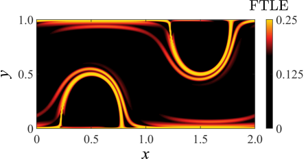
Figure 2: Forward FTLE field showing LCS structure of the unperturbed kinematic system with $\epsilon=0$.

Figure 2 shows the forward FTLE field for the unperturbed system $\mathbf{f}(\mathbf{x},t)$ on the non-dimensional grid $[0,2]\times[0,1]$. Two dominant horseshoe ridges centered at $x=0.5$ (lower left) and $x=1.5$ (upper right) are observed. Fluid particles outside the horseshoe boundaries generally travel in the positive $x$ direction due the background flow $U_{0}$. In contrast, particles inside the horseshoe structures do not exit and continuously circulate.

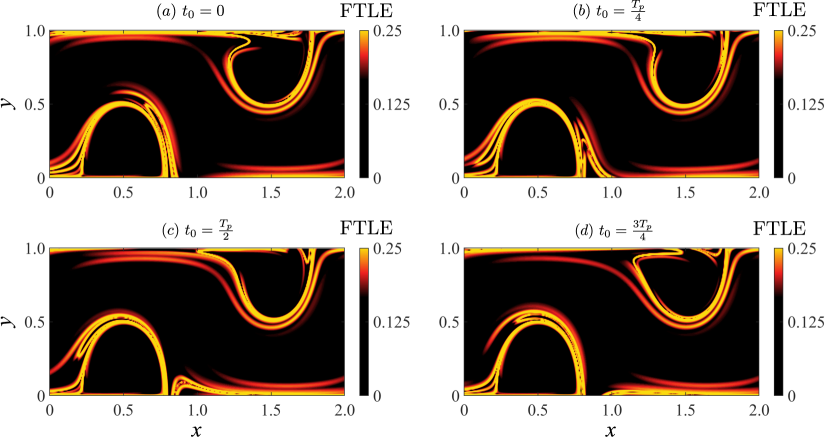
Figure 3: LCS structure of the perturbed kinematic system $f(x,t)+\epsilon g(x,t)$ for various initial times $t_{0}$ with $\epsilon=0.03$.

Applying the perturbation $\mathbf{g}(\mathbf{x},t)$ with $\epsilon=0.03$, as in figure 3, creates additional loops around the lower-left horseshoe and deform the upper-right horseshoe. Despite the moderate effects from the perturbations, the original features from the FTLE field in figure 2 are retained in figure 3.

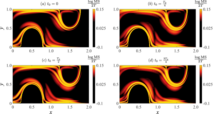
Figure 4: Mode sensitivity ($\mathrm{MS}_{t_{0}}^{t}$) structure of the perturbed kinematic system for various initial times $t_{0}$ with $\epsilon=0.03$.

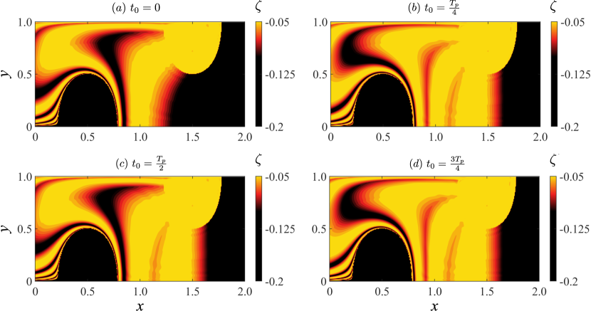
Figure 5: Perturbations ($\zeta_{t_{0}}^{t}$) to the FTLE flow field in figure 2 at various phases ($T_{p}=5$) with $\epsilon=0.03$.

Regions where the LCS should change from the perturbation $\mathbf{g}(\mathbf{x},t)$ are indicated by the MS field in figure 4. High MS values coincide with the lobe perturbations observed for the lower-left horseshoe. High MS values near the upper-right boundary represent the locations where deformation of the LCSs is expected.

Since the baseline system is steady in this case, the time dependence of the MS field arises solely from the perturbation amplitude, $\Delta_{\infty}$. This unsteadiness is observed in the perturbation field defined in equation (17). Note how from $t=0$ and $t=3T/4$, the magnitude of the MS field rises around the upper-right horseshoe ($x\approx 1.5$). An increase in the MS magnitude reflects the perturbations experienced by particles in subsequent times. This can be further observed in the FTLE perturbation field $\zeta_{t_{0}}^{t}$ in figure 5. Because the perturbation $\mathbf{g}(\mathbf{x},t)$ acting in the $y$ direction is centered at $x=d=1.4$, the magnitude of $\zeta_{t_{0}}^{t}$ increases rapidly across the $y$-axis at this location. Additional transient characteristics of the perturbation field include the sharp bands around the lower-left horseshoe that travel in the positive $x-$direction. These are responsible for forming the traveling lobes around the lower-left horseshoe in the MS field (figure 4) and the perturbed FTLE field (3). These results are illustrative for offering insight into the effects of introduced perturbations on the initial LCS structures.

3 Mode Sensitivity

We now consider a particular definition of model sensitivity in the context of modal decomposition. A detailed overview of modal analysis techniques is provided by Taira et al. [2020] and Rowley and Dawson [2017]. Consider a set of snapshots of velocity, $\mathbf{u}(\mathbf{x},t)$, which can be have either two or three-dimensions. The general aim of modal representations is to take the high dimensional dataset $\mathbf{u}$ and compress the data into a lower dimensional form $\hat{\mathbf{u}}$ that represents the main dynamics. Thus, $\hat{\mathbf{u}}$ is expressed as a limited set of $r$ linearly independent modes (i.e., a rank $r$ approximation):

$$\mathbf{u}\approx\hat{\mathbf{u}}=\sum_{k=1}^{r}a_{k}\boldsymbol{\psi}_{k},$$ (23)

where $\psi_{k}$ is the spatial basis function (i.e., a POD or DMD mode) with a corresponding amplitude coefficient $a_{k}$. Now consider that the dynamics of passive tracer particles in the flow field can be given by:

$$\frac{d\mathbf{x}}{dt}=\mathbf{u}(\mathbf{x},t).$$ (24)

Combining the above equation with equation (3), we can then express the set of modes as a combination of dynamical systems $\mathbf{f}(\mathbf{x},t)$ and $\mathbf{g}(\mathbf{x},t)$:

$$\frac{d\mathbf{x}}{dt}=\mathbf{u}(\mathbf{x},t)\approx\sum_{k=0}^{r}a_{k}\boldsymbol{\psi}_{k}=\mathbf{f}(\mathbf{x},t)+\epsilon\mathbf{g}(\mathbf{x},t),$$ (25)

where $\mathbf{f}(\mathbf{x},t)$ and $\epsilon\mathbf{g}(\mathbf{x},t)$ can each represent a linear combination of modes in different combinations so long as $|\epsilon\mathbf{g}|\ll|\mathbf{f}|$. Thus, if $\epsilon$ is small enough such that $\mathbf{f}(\mathbf{x},t)$ contains most of the dynamics in $\mathbf{f}(\mathbf{x},t)+\epsilon\mathbf{g}(\mathbf{x},t)$, we can quantify this contribution by considering the ratio:

$$\epsilon=\frac{||\epsilon\mathbf{g}(\mathbf{x},t)||_{F}}{||\mathbf{f}(\mathbf{x},t)||_{F}},$$ (26)

where $||\cdot||_{F}$ represents the Frobenius norm. We note that as long as $\epsilon\mathbf{g}(\mathbf{x},t)$ can be defined by a certain number of modes from equation 25, the above equation can be computed without the knowledge of $\epsilon$ apriori.

Depending on the dataset $\mathbf{u}(\mathbf{x},t)$ and the modal decomposition method used, the definition of mode components in $\epsilon\mathbf{g}(\mathbf{x},t)$ relative to the full system $\mathbf{f}(\mathbf{x},t)+\epsilon\mathbf{g}(\mathbf{x},t)$ can be framed in a variety of ways. For instance, the primary or baseline dynamical system $\mathbf{f}(\mathbf{x},t)$ can represent a highly truncated modal representation and $\epsilon\mathbf{g}(\mathbf{x},t)$ can represent the neglected modes. Further, variants of the decomposition methods described by equation (23) lead to different basis functions $\boldsymbol{\psi}_{k}$, and thus different expressions for $\mathbf{f}(\mathbf{x},t)$ and $\epsilon\mathbf{g}(\mathbf{x},t)$. The Proper Orthogonal Decomposition (POD) [Berkooz et al., 1993] for example uses orthonormal spatial basis vectors for the modes. In this case, the basis vectors of equation 25 follow the condition:

$$\langle\boldsymbol{\psi}_{i},\boldsymbol{\psi}_{j}\rangle=\int_{\Omega}\boldsymbol{\psi}_{i}(\mathbf{x})\boldsymbol{\psi}_{j}(\mathbf{x})\,d\mathbf{x}=\begin{cases}1&\text{if }i=j\\ 0&\text{if }i\neq j\end{cases}$$ (27)

Alternatively, Dynamic Mode Decomposition (DMD) as introduced by Schmid [2010] consist of basis vectors such that each mode contains a particular frequency and growth rate. For a reconstruction of $\mathbf{u}$ based on DMD modes, equation (23) becomes:

$$\hat{\mathbf{u}}=\sum_{k=0}^{r}b_{k}\exp{(\omega_{k}t)}\boldsymbol{\psi}_{k},$$ (28)

where $b_{k}$ is the mode amplitude coefficient and $\omega_{k}$ is the eigenvalue corresponding to the vector $\boldsymbol{\psi}_{k}$.

We aim to characterize how the Eulerian modes of $\epsilon\mathbf{g}(\mathbf{x},t)$ influence the LCS. For the remainder of this paper, therefore, the term Model Sensitivity (MS) can be interpreted as Mode Sensitivity. In this context, the term $\zeta$ in equation (16) can be thought of as a Lagrangian response that characterizes the sensitivity of the LCS field specifically to the modes in $\mathbf{g}(\mathbf{x},t)$.

For the unsteady shear flows considered in this paper, most decomposition methods explicitly yield a mean (or time-averaged) flow as one of the leading modes. Often, the the mean flow contains more energy (in the $L_{2}$ sense) than other modes. Thus, for all cases in this study, we will consider the mean flow $\bar{\mathbf{u}}$ as part of the main dynamical system $\mathbf{f}(\mathbf{x},t)$.

One property that must be considered for the amplitude uncertainty $\Delta_{\infty}$ in equation (12) is the error bound due to the superposition of modes. For example, consider contributions from two modes $\mathbf{u}_{n}$ and $\mathbf{u}_{m}$ which do not follow any particular order. One can compute the term $\Delta_{\infty}$ using either $\mathbf{u}_{n}$ and $\mathbf{u}_{m}$ separately as:

$$\Delta_{\infty}^{\mathbf{u}_{n}}=\epsilon\max\limits_{s\in[t_{0},t]}|\mathbf{u}_{n}(\mathbf{x}^{0}(s),s))|,$$ (29)

and

$$\Delta_{\infty}^{\mathbf{u}_{m}}=\epsilon\max\limits_{s\in[t_{0},t]}|\mathbf{u}_{m}(\mathbf{x}^{0}(s),s))|,$$ (30)

or as a combination of modes:

$$\Delta_{\infty}^{\mathbf{u}_{n}+\mathbf{u}_{m}}=\epsilon\max\limits_{s\in[t_{0},t]}|\mathbf{u}_{n}(\mathbf{x}^{0}(s),s)+\mathbf{u}_{m}(\mathbf{x}^{0}(s),s)|.$$ (31)

Using the triangle inequality $|\mathbf{u}_{n}+\mathbf{u}_{m}|\leq|\mathbf{u}_{n}|+|\mathbf{u}_{m}|$, the amplitude and trajectory uncertainties can then be bounded as:

$$\Delta_{\infty}^{\mathbf{u}_{n}+\mathbf{u}_{m}}\leq\Delta_{\infty}^{\mathbf{u}_{n}}+\Delta_{\infty}^{\mathbf{u}_{m}},$$ (32)

and

$$\epsilon|\boldsymbol{\eta}|\leq\Delta_{\infty}^{\mathbf{u}_{n}+\mathbf{u}_{m}}\int_{t_{0}}^{t}\sqrt{\lambda_{s}^{t}(\mathbf{x}^{0}(s))}ds\leq\left(\Delta_{\infty}^{\mathbf{u}_{n}}+\Delta_{\infty}^{\mathbf{u}_{m}}\right)\int_{t_{0}}^{t}\sqrt{\lambda_{s}^{t}(\mathbf{x}^{0}(s))}ds.$$ (33)

Thus, an upper bound for the sensitivity field can be computed by adding the amplitude uncertainty associated with individual modes in $\epsilon\mathbf{g}(\mathbf{x},t)$. From a physical perspective, the above inequalities arise from the fact that superimposing modes in both time and space can result in lower magnitudes in comparison to the the sum of their absolute values.

3.1 Computing the MS field

Often, flow fields acquired from numerical simulations or experiments have a limited interrogation region. Pertinent to the FTLE and MS calculations, this affects how long passive tracers are advected before exiting the domain. One approach for circumventing this issue is to select a subdomain to initialize the passive tracers in the existing data. However, this is typically not a full solution since it is preferred that the integration $T$ must be long enough for a sufficient number of particles to exit the subdomain. Another practical approach is to assign particles that exit the domain an approximation of the velocity, based on the appropriate boundary conditions from the data [Rockwood et al., 2019].

For flow fields that have a dominant advection direction, passive tracers that exit a distance $\Delta\mathbf{x}$ from the domain can continue to advect based on the mean flow field, expressed as:

$$\mathbf{u}(\mathbf{x}+\Delta\mathbf{x},t)=\bar{\mathbf{u}}(\mathbf{x},t).$$ (34)

Alternatively, one may use Taylor’s frozen eddy hypothesis, which assumes that a passive tracer that exits the domain a distance $\mathbf{x}+\Delta\mathbf{x}$ and earlier time $t$ experiences the same velocity at a distance $\mathbf{x}$ and time $t-\frac{\Delta x}{u_{a}}$; that is:

$$\mathbf{u}(\mathbf{x}+\Delta\mathbf{x},t)=\mathbf{u}\left(\mathbf{x},\ t-\frac{\Delta x}{u_{a}(\mathbf{x},\ t)}\right),$$ (35)

where $u_{a}$ is an advection speed. In the following sections, we compute the Lyapunov exponent $\lambda_{s}^{t}$ in equation (13) using equation (34) to approximate particle trajectories that exit the domain. Similarly, the computation of $\Delta_{\infty}$ also requires a flow field approximation for particles that leave the domain due to the limited domain of the perturbation $\epsilon\mathbf{g}(\mathbf{x},t)$. Unless stated otherwise, the values of $\epsilon\mathbf{g}(\mathbf{x},t)$ were extrapolated using Taylor’s frozen eddy hypothesis as in equation (35).

4 Applications and Results

4.1 Example 2: Flow past the wake of an oscillating foil

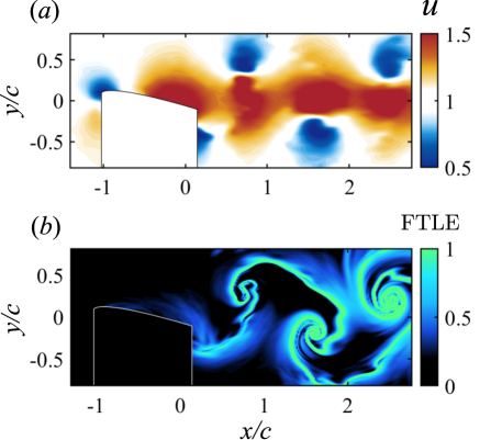
Figure 6: ($a$) Streamwise velocity field from an oscillating foil ($St=0.29$) and ($b$) backward FTLE structure at the phase $t=T_{p}/4$.

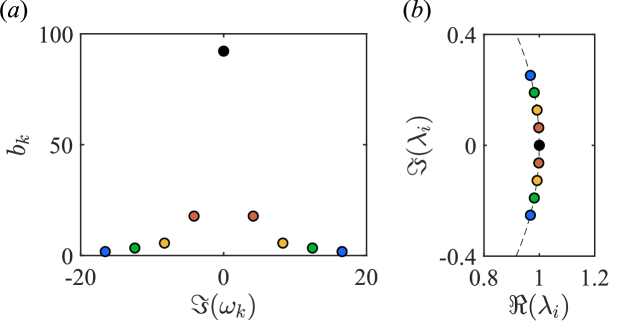
Figure 7: ($a$) amplitude and ($b$) eigenvalue spectrum of the opt-DMD modes for the flow past an oscillating foil. The modes pair are highlighted in red ($\mathbf{u}_{1}$), orange ($\mathbf{u}_{2}$), green ($\mathbf{u}_{3}$), and blue ($\mathbf{u}_{4}$). The mean flow highlighted in black is denoted as $\bar{\mathbf{u}}$.

We first show how the mode sensitivity field is useful for the analysis of vortex-dominated flows. In particular, we use Particle Image Velocimetry (PIV) data for the wake of an oscillating foil at a Strouhal number of $St=\omega A/2\pi U_{\infty}=0.29$ from Jones et al. [2024]. Here, $\omega$ is the oscillation frequency, $A$ is the amplitude of oscillation at the trailing edge and $U_{\infty}$ is the freestream velocity. This oscillation frequency results in peak propulsive efficiency for fixed heave and pitch amplitudes, and a constant phase difference between the sinusoidal pitching and heaving motions. PIV data were obtained in the wake of the oscillating foil over the domain $(x/c,\ y/c)\in[0.35,\ 2.76]\times[-0.82,\ 0.82]$, where the coordinates are relative to the tip of the foil at pitch angle and heave position of $0^{\circ}$ and $0$ respectively, and $c$ is chord length. An additional field-of-view centered on the foil was used to better capture the wake structures produced around the foil. A dynamic mask was used to remove erroneous velocity vectors within or near the foil region. After removing erroneous velocity vectors, both datasets were combined in post-processing using a moving-average filter to reduce the signal-to-noise ratio. The combined data extended the PIV domain to $(x/c,\ y/c)\in[-2,\ 2.76]\times[-0.82,\ 0.82]$ and contained $141\times 49$ velocity vectors. The streamwise component of the combined flow field is shown in figure 6($a$).

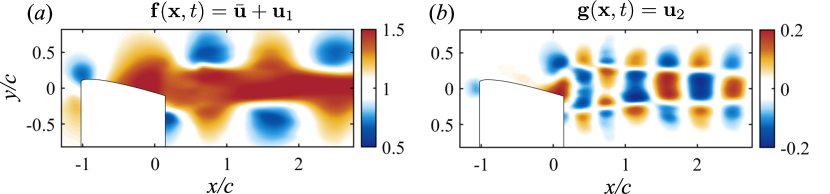
Figure 8: Streamwise component for a) the primary flow field and b) mode perturbation for the flow past an oscillating foil at the phase $t=T_{p}/4$.

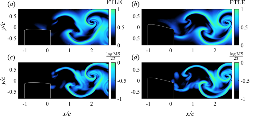
Figure 9: LCSs of the flow past an oscillating foil for the system $\mathbf{f}(\mathbf{x},t)$ ($a,b$) as described in equation (36) and ($c,d$) Mode sensitivity fields at the phases (left) $t=0$ and (right) $t=T_{p}/4$.

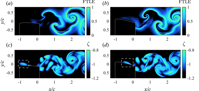
Figure 10: LCSs of the flow past an oscillating foil for the system $\mathbf{f}(\mathbf{x},t)+\epsilon\mathbf{g}(\mathbf{x},t)$ ($a,b$) as described in equation (36) and ($c,d$) Lagrangian response fields at the phases (left) $t=0$ and (right) $t=T_{p}/4$. The dashed box highlights a component of the leading edge vortex.

The aim in this example is to understand how particular modes that relate to high propulsive efficiency affect the LCS structure. Previous work [Jones et al., 2024] showed that opt-DMD modes obtained from this flow field highlight thrust and drag producing effects at different Strouhal numbers, $St$. Here, we use the same opt-DMD method for the combined dataset. The spectrum of opt-DMD modes is shown in figure 7. The four leading unsteady modes, ordered in terms of frequency, are denoted $\mathbf{u}_{1}-\mathbf{u}_{4}$. Consistent with the previous study, the primary mode $\mathbf{u}_{1}$ for this dataset corresponds to the oscillation frequency of the foil and, together with the mean flow $\bar{\mathbf{u}}$, represents a majority of the wake dynamics. The secondary mode $\mathbf{u}_{2}$ contributes to the shear layer roll up of the vortices.

For this Strouhal number case, both $\mathbf{u}_{1}$ and $\mathbf{u}_{2}$ yielded positive induced velocities in the wake (i.e., contributed to thrust generation) and high efficiency. Because we are interested in characterizing the effect of mode $\mathbf{u}_{2}$ on the primary LCS structure of the wake, we choose the unperturbed dynamical system and the perturbation to be

$$\mathbf{f}(\mathbf{x},t)=\boldsymbol{\bar{\mathbf{u}}(x)}+\mathbf{u}_{1}(\mathbf{x},t),\ \ \ \epsilon\mathbf{g}(\mathbf{x},t)=\mathbf{u}_{2}(\mathbf{x},t).$$ (36)

The streamwise velocity components ($u$) for these flow fields are shown in figure 8. Note that the amplitude coefficients for the mean flow $\bar{\mathbf{u}}$ and modes $\mathbf{u}_{1}-\mathbf{u}_{2}$ are $b_{0}=72.3$, $b_{1}=34.2$, and $b_{2}=10.6$ respectively. Following equation (32), the corresponding value of $\epsilon$ for equation (36) can be estimated as $\epsilon\approx 0.1$. In other words, mode $\mathbf{u}_{2}$ represents a small amplitude perturbation to the baseline flow field. However, as shown below, it does modify the FTLE field in a meaningful way.

LCS and MS fields for this dataset are computed in backward time, (FTLE${}_{t}^{t_{0}}$ and $MS_{t}^{t_{0}}$). Given the uniform flow field upstream, we assume that particles that exit the limited domain in the negative $x-$direction and either $y-$direction experience a perturbation of $\epsilon\mathbf{g}=0$, and a freestream velocity of $u_{\infty}=1$. These assumptions are used to approximate the amplitude $\Delta_{\infty}$.

The backward FTLE field for the original (full) flow field is shown in figure 6($b$). Vortex roll-up is observed where the manifolds spiral inwards, as also found from the results of [Green et al., 2011]. The FTLE field for the baseline (unperturbed) velocity field is shown in figures 9$(a,b)$, which comprises the mean flow and the first leading modal contribution. A set of weakened vortex rollers are observed in this reduced model. As expected, the mode sensitivity fields in figures 9$(c,d)$ effectively reflect the dynamics of original FTLE field. Specifically, the MS field highlights the lower spiral which is weakened in the reduced model as well as the sections of the shear layers that show reduced undulation. These effects from the secondary mode $\mathbf{u}_{2}$ on the wake structure are further highlighted in figures 10$(a,b)$, where adding the mode strengthens the roll-up and leads to increased corrugation of the shear layer.

The response field $\zeta$ (figures 10$c,d$) provides additional insight into how mode $\mathbf{u}_{2}$ relates to the flow structure. Notably, components of the leading edge vortex are observed close to the foil which advect into the LCS structure downstream. This particular feature is not present in any of the FTLE fields presented. The Lagrangian response $\zeta$ suggests that the leading edge vortex advecting into the wake contributes to the shear layer corrugation present in both the perturbed model $\mathbf{f}(\mathbf{x},t)+\epsilon\mathbf{g}(\mathbf{x},t)$ (figures LABEL:fig:osc-ftle-pert$a,b$) and the original flow field (figure 6$b$). Indeed, the $\zeta$ fields capture both the intensification of the vortex roll-up (see e.g., $x/c\approx 1.0-1.5$ and $y/c<0$) and the corrugation of the shear layer. These physical insights complement prior work [e.g., Quinn et al., 2015, Lentink et al., 2008] aiming to characterize the impact of local flow features around oscillating foils on the downstream wake structure. In general, these results show that the MS and $\zeta$ fields serve as useful tools for finding specific Eulerian flow features in relation to Lagrangian transport.

4.2 Example 3: Flow past the wake of a circular cylinder

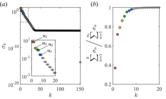
Figure 11: ($a$) SVD spectrum and ($b$) cumulative energy spectrum for the cylinder wake. The dotted line is the zoomed-in plot in ($a$), highlighting the mode pairs in red ($\mathbf{u}_{1}$), orange ($\mathbf{u}_{2}$), green ($\mathbf{u}_{3}$), and blue ($\mathbf{u}_{4}$).

Next, we study the mode sensitivity of the canonical cylinder wake flow ($Re=u_{\infty}d/\nu=100$ and $St=0.16$) from Kutz et al. [2016], where d is the cylinder diameter. The simulation was developed using an immersed boundary projection method fluid solver, as described by Taira and Colonius [2007]. Data were obtained over a dimensionless subdomain of $(x,y)\in[-1,\ 8]\times[-2,\ 2]$ and constituted a grid of $449\times 199$ velocity vectors. POD was used on this dataset for the mode sensitivity analysis. The POD modes were then interpolated in time using a Makima spline to increase the number of snapshots from $n_{t}=151$ ($\Delta t=0.2u_{\infty}/d$) to $n_{t}=755$ ($\Delta t=0.04u_{\infty}/d$). This increased time resolution in the data improves the accuracy for particle trajectories and the computation of $\Delta_{\infty}$. The approach is reasonable for approximating times in between the sampled snapshots because the modes for this flow field are linear. The spectrum of the POD modes is shown in figure 11. The mode pair with the highest energy (denoted as $\mathbf{u}_{1}$) corresponds to the shedding frequency of the wake, while subsequent modes are higher-order harmonics [Taira et al., 2020]. To better understand how the harmonic modes affect the vortex street, we consider the two different perturbed systems, representing different levels of model reduction, for the mode sensitivity analysis:

$$\mathbf{f}(\mathbf{x},t)=\bar{\mathbf{u}}(\mathbf{x})+\mathbf{u}_{1}(\mathbf{x},t)+\mathbf{u}_{2}(\mathbf{x},t),\ \ \ \epsilon\mathbf{g}(\mathbf{x},t)=\mathbf{u}_{3}(\mathbf{x},t),$$ (37)

and

$$\mathbf{f}(\mathbf{x},t)=\bar{\mathbf{u}}(\mathbf{x})+\mathbf{u}_{1}(\mathbf{x},t)+\mathbf{u}_{2}(\mathbf{x},t)+\mathbf{u}_{3}(\mathbf{x},t),\ \ \ \epsilon\mathbf{g}(\mathbf{x},t)=\mathbf{u}_{4}(\mathbf{x},t).$$ (38)

The primary flow fields $\mathbf{f}(\mathbf{x},t)$ and the perturbations $\epsilon\mathbf{g}(\mathbf{x},t)$ for these two cases are shown in figure 12. Similar to the case of the oscillating foil in section 4.1, we compute the FTLE and mode sensitivity fields in backward time, using the same assumptions for approximating the velocity field outside the domain.

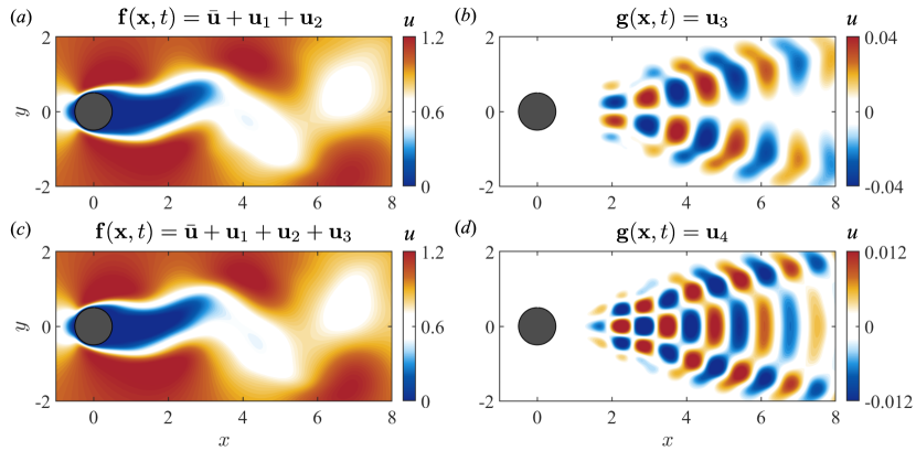
Figure 12: streamwise velocity of the primary fluid structures $\mathbf{f}(\mathbf{x},t)$ and perturbations $\epsilon\mathbf{g}(\mathbf{x},t)$ used for the sensitivity of the cylinder wake. ($a,b$) First and ($c,d$) second mode sensitivity cases.

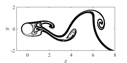
Figure 13: Dominant backward FTLE structure original flow field for the cylinder wake. Backward FTLE values that were less than 38% of the max value were removed.

The backward FTLE field of the original flow field is shown in figure 13, illustrating the dynamics of the classical von Karman vortex street. Figure 14 considers the effect of model reduction on the FTLE fields for this narrow-banded flow. Figure 14($a,c$) in the left column shows the Lagrangian response $\zeta$ of the FTLE field. Note that the full field of $\zeta$ covers a wide region in the vortex street. To find where these perturbations overlap with the dominant manifolds, we superimpose the response $\zeta$ onto the FTLE field for the baseline systems $\mathbf{f}(x,t)$ (described in equations 37–38). Thus, from figures 14($b,d$), we observe that mode $\mathbf{u}_{3}$ shifts the FTLE ridges between the vortices by a subtle amount and moves the roll-up of the vortices closer to the centerline $y=0$. This response is highlighted in the regions where the baseline FTLE fields coincide with large values of $\zeta$ in figure 14$b$. The response field in 14$d$ suggests that mode $\mathbf{u}_{4}$ improves the roll up by an even smaller margin, as expected from the energy of distribution in figure 11$b$. Thus, both modal representations contain the LCS dynamics of the flow field reasonably well.

Recall that the MS field combines information from the baseline FTLE field as well as the Lagrangian response to the disturbance $\zeta$. The cylinder flow results further confirm that the response field $\zeta$ is useful for identifying local effects from individual modes, particularly when interpreted in conjunction with the sharp and narrow FTLE ridges of the baseline system, $\mathbf{f}(\mathbf{x},t)$.

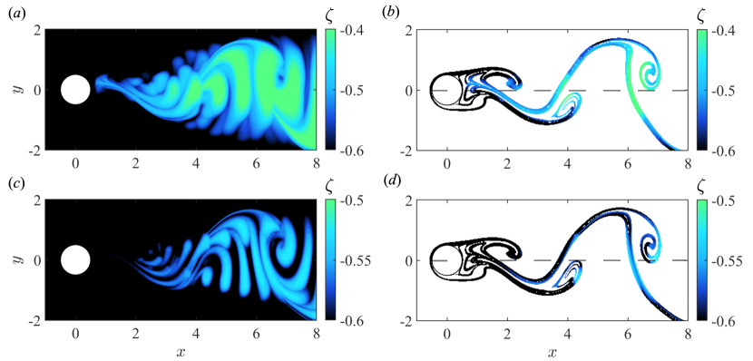
Figure 14: (left) Lagrangian responses $\zeta$ for the cylinder wake flow field. (right) Magnitudes of $\zeta$ superposed onto the backward FTLE field for the baseline flow field $\mathbf{f}(x,t)$. Backward FTLE values that were less than 38% of the max value were removed. Each row corresponds to the flow structure cases in figure 12. The dotted line is the center line of the flow field ($y=0$).

4.3 Example 4: Turbulent channel flow

The previous sections have demonstrated the utility of the MS framework in the context of model reduction. Here, we use it to highlight the effect of specific dynamically important features (or modes) on LCS for a flow field with broadband length and time scales.

In particular, we use turbulent channel flow with a friction Reynolds number $Re_{\tau}=u_{\tau}h/\nu=1000$ from the John Hopkins Turbulence Database [Graham et al., 2016], where $u_{\tau}$ is the friction velocity and $h$ is the channel half height. Two-dimensional data were extracted over the domain of $(x,y)\in[-\pi,\ 3\pi]\times[-1,\ 1]$ and yielded $1024\times 160$ velocity vectors. Here, the dimensions are normalized by $h$. A set of $n_{t}=565$ snapshots were extracted with a time step of $\Delta t=0.02h/u_{b}$, where $u_{b}$ is the bulk velocity. Figure 15a shows the streamwise component of the velocity field for the first snapshot. We recognize that the use of a two-dimensional (2D) slice for LCS analyses is a substantial simplification as out-of-plane motion can significantly alter particle trajectories. However, prior work from [Green et al., 2007] has shown that this 2D approximation still provides substantial insight.

Tracer particles were advected for an integration time of $T=2.9$ in the subdomain of $(x,y)\in[0,\ 2\pi]\times[-1,\ 1]$. The initial grid comprised $514\times 160$ particles. The selected subdomain allows for a majority of the particles to advect with the velocity field before exiting the domain at $x=3\pi$. Particles that exited the domain early continued to advect with the time-averaged flow field (as in equation 34) at the respective $y-$location. The forward FTLE field of the original flow field is shown in figure 15$b$, small-scale filament structures that are observed.

Research over the past two decades has highlighted the energetic and dynamic importance of the so-called Large-Scale Motions (LSMs) and Very Large Scale Motions (VLSMs) on wall bounded turbulent flows [Hutchins and Marusic, 2007, Marusic et al., 2010]. It has been shown that LSMs and VLSMs have increasing spectral contributions as the Reynolds number increases, and that these large-scale structures have an organizing influence on small-scale turbulence [Marusic et al., 2010]. VLSMs exhibit streamwise coherence over distances of up to 30 times the channel half-height (typically $6-10h$), while LSMs have streamwise length scales of 2-3 times the channel half-height [Smits et al., 2011]. Previous studies have shown that modal analysis techniques such as SPOD and resolvent analysis can effectively capture these large-scale structures [Towne et al., 2022, Saxton-Fox et al., 2022]. The aim in this example is to use mode sensitivity to understand how these large scale structures influence smaller scale features.

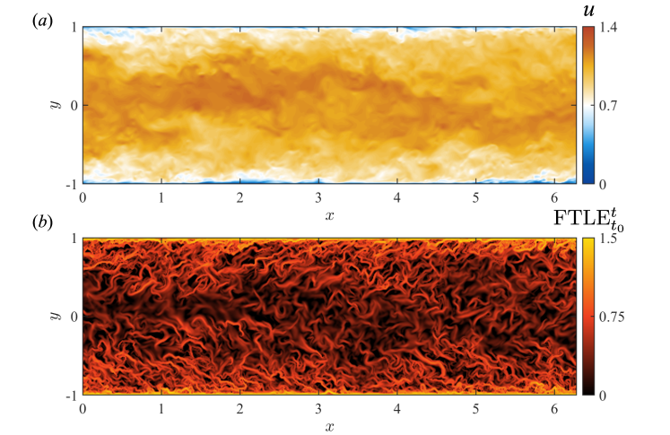
Figure 15: ($a$) Streamwise velocity component of the turbulent channel flow field at $t=0$ and ($b$) the corresponding forward FTLE field.

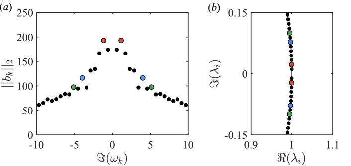
Figure 16: ($a$) Amplitude and ($b$) eigenvalue spectrum of the DMD modes for the turbulent channel flow field. The mode pairs highlighted in red ($\Im(\omega)=1.1$), blue ($\Im(\omega)=4.0$), and green ($\Im(\omega)=5.1$) are separately chosen as the perturbations $\epsilon\mathbf{g}(\mathbf{x},t)$.

For the present data, we use the DMD algorithm on the full domain to extract the large-scale structures of interest. As a result of the spatial homogeneity and statistical stationarity expected in channel flow, it should be expected that the modes neither grow or decay in time or space (specifically the streamwise direction). We therefore perform DMD on the dataset with the time-averaged flow field subtracted, which results in decay rates of 0 for all modes. The modes obtained are therefore equivalent to that from a temporal Fourier transform [Chen et al., 2012].

As considered in the previous examples, we treat modes with the same oscillation frequency as pairs. Several local peaks in amplitude for each mode pair are highlighted in figure 16. These modes have streamwise wavelengths of $\lambda_{x}/h\approx 6,\ 1.5-2.0$, and $1.0$, where $h$ is the channel half-height, as shown in figure 17. These wavelengths may be reminiscent of VLSMs and LSMs that affect the smaller scale LCS filaments in figure 15$b$. To better understand this interaction, we consider three separate mode sensitivity cases, where each of the highlighted mode pairs, denoted as $\mathbf{u}_{s}$, are considered as the perturbation $\mathbf{g}$ in three separate cases. The main fluid structure $\mathbf{f}(\mathbf{x},t)$ and perturbation $\mathbf{g}(\mathbf{x},t)$ are constructed as:

$$\mathbf{f}(\mathbf{x},t)=\bar{\mathbf{u}}(\mathbf{x})+\sum_{\begin{subarray}{c}k=1\\ k\neq s\end{subarray}}^{n_{t}}\mathbf{u}_{n}(\mathbf{x},t),\ \ \ \mathbf{g}(\mathbf{x},t)=\mathbf{u}_{s}(\mathbf{x},t),$$ (39)

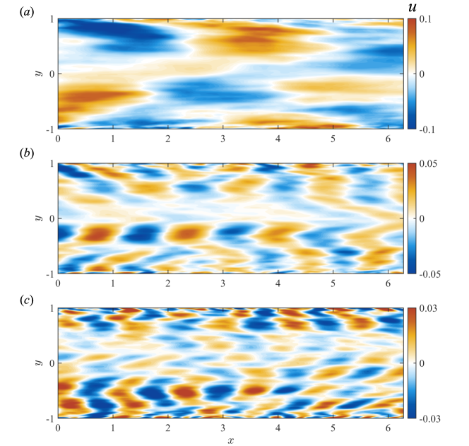
Figure 17: Mode structures for the turbulent channel flow field with the following wavelengths and frequencies: ($a$) $\Im(\omega)=1.1$,  $\lambda_{x}/h\approx 6$,  ($b$) $\Im(\omega)=4.0,\ \lambda_{x}/h\approx 1.5-2.0$,  ($c$) $\Im(\omega)=5.1,\ \lambda_{x}/h\approx 1.0$.

for each case, where $n_{t}$ are the total number of modes. We note how this constructed model differentiates from the periodic flow field examples since we consider an eigenvalue decomposition on the data with all snapshots rather than that on a truncated linear operator $\tilde{A}$ described by Tu et al. [2014], which may filter out some important length scales.

Regions where the smaller scale structures are affected by these modes are shown in figure 18. While the FTLE field in figure 15$b$ highlights persisting ridges of sensitivity in all locations, the MS field results in more robust structures for each case and focuses on ridges that are influenced by the mode structure $\mathbf{u}_{s}$. The structures that are most sensitive to each of the modes are closest to the walls of the channel, which may suggest that most of the energy in these modes attenuate the small scale features in the inner region, while the remaining energy amplifies the LCSs in the outer region. The results compliment the observations found in experiments and simulations on the organization between small and large scale structures [Hutchins and Marusic, 2007, Chung and McKeon, 2010, Howland and Yang, 2018].

Patches of the mode structures can be more clearly seen in the Lagrangian response field $\zeta$ (figure 18$c$). Higher magnitudes are concentrated closer to the wall for the case of $\lambda_{x}/h\approx 6$, compared to the smaller-wavelength modes ($\lambda_{x}/h\approx\ 1.5-2.0$, and $1.0$), as expected from the amplitudes coefficient. However, since the MS defines the upper bound where FTLE fields change due to finite perturbations, these smaller-wavelength modes could potentially affect the LCS filaments close to the wall more than the mode with $\lambda_{x}/h\approx 6$. The observations of these fields show that both the MS and Lagrangian responses effectively isolate both the regions and the specific streaks that VLSMs and LSMs may affects in the LCS.

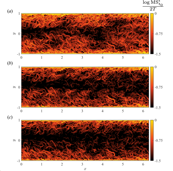
Figure 18: Mode sensitivity of dominant structures for the turbulent channel flow. ($a$) $\Im(\omega)=1.1$,  $\lambda_{x}/h\approx 6$,  ($b$) $\Im(\omega)=4.0,\ \lambda/h\approx 1.5-2.0$,  ($c$) $\Im(\omega)=5.1,\ \lambda_{x}/h\approx 1.0$.

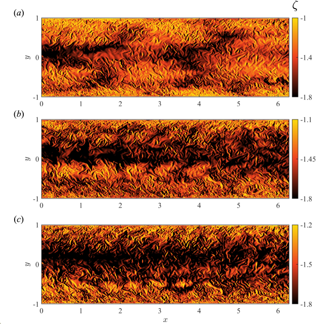
Figure 19: FTLE perturbation fields $\zeta$ of dominant structures for the turbulent channel flow. Modes are ordered as in figure 17.

5 Discussion and Conclusions

This paper presents an algorithm for finding dominant LCSs that are affected by mode structures. The framework yields two important flow field metrics: 1) The mode sensitivity field (MS) which highlights parts of the LCS structure in the fluid flow that a given mode $\epsilon\mathbf{g}(\mathbf{x},t)$ is likely to affect, and 2) the Lagrangian response $\zeta$ which provides more explicit details on where the mode perturbs the FTLE field. While these coherent structures relate to the FTLE, their patterns pertain more to the dynamic interactions between the mode and the LCS, adding a new perspective to modal decompositions.

The method is demonstrated on both experimental and numerical data, with a focus towards understanding cross-stream perturbations, shear layer instabilities, and LSMs and VLSMs in turbulent flows. For these examples, and many other fluid flows that are not presented in this paper (e.g., stationary or isotropic flows), the choice of the reconstructed flow field $\mathbf{f}(\mathbf{x},t)$ (as defined in equation (25)) has considerable flexibility, as it is not limited to one modal representation. Although it should be ensured that $\mathbf{f}(\mathbf{x},t)$, and hence its FTLE field, contains a majority of the dynamics from the original flow field. Consequently, the definition of the perturbation $\epsilon\mathbf{g}(\mathbf{x},t)$ used in mode sensitivity can also be openly defined, such as a single mode or a collection of modes with different dynamical properties (e.g, frequencies, growth rates, topologies etc). The examples considered in this paper considered perturbations as modes pairs based on conjugate eigenvalues. The method can also be extended to other decomposition methods that use different basis functions from the POD or DMD algorithm.

An important aspect of the Lagrangian response $\zeta$ is that it represents the Eulerian modes in a different feature space. For example, while decomposition approaches derived from stability analyses often represent mode perturbations with respect to a mean flow structure, the Lagrangian response represents perturbations to the FTLE flow structure of $\mathbf{f}(\mathbf{x},t)$. In two of these examples, we use the DMD algorithm, which enforces each mode with a frequency of oscillation and growth rate. The corresponding Lagrangian response may not entirely preserve these characteristics, but rather, represents DMD modes in a feature space based on the FTLE structure. This transformation space may have useful implications for flow control applications.

The mode sensitivity analysis can also be expanded to mode truncations or filtered computational models such as Large-Eddy Simulations, which may be useful for quantifying uncertainty in flow dynamics. It is worth noting that the algorithm is computationally expensive when applied to three-dimensional flow fields. Approximate methods such as the flow map composition can improve the speed by avoiding redundant computations of the flow map [Brunton and Rowley, 2010]. The presented method is robust to both experiments and simulations and may serve as a tool to help better understand how modes obtained from data driven decomposition techniques affect the coherent structure of the complete flow field.

References

- Berkooz et al. [1993] G. Berkooz, P. Holmes, and J. L. Lumley. The Proper Orthogonal Decomposition in the Analysis of Turbulent Flows. Annual Review of Fluid Mechanics, 25(1):539–575, Jan. 1993. ISSN 0066-4189, 1545-4479. doi: 10.1146/annurev.fl.25.010193.002543. URL https://www.annualreviews.org/doi/10.1146/annurev.fl.25.010193.002543.
- Brauer [1966] F. Brauer. Perturbations of nonlinear systems of differential equations. Journal of Mathematical Analysis and Applications, 14(2):198–206, May 1966. ISSN 0022-247X. doi: 10.1016/0022-247X(66)90021-7. URL https://www.sciencedirect.com/science/article/pii/0022247X66900217.
- Brunton and Noack [2015] S. L. Brunton and B. R. Noack. Closed-Loop Turbulence Control: Progress and Challenges. Applied Mechanics Reviews, 67(5):050801, Sept. 2015. ISSN 0003-6900, 2379-0407. doi: 10.1115/1.4031175. URL https://asmedigitalcollection.asme.org/appliedmechanicsreviews/article/doi/10.1115/1.4031175/369906/ClosedLoop-Turbulence-Control-Progress-and.
- Brunton and Rowley [2010] S. L. Brunton and C. W. Rowley. Fast computation of finite-time Lyapunov exponent fields for unsteady flows. Chaos: An Interdisciplinary Journal of Nonlinear Science, 20(1):017503, Mar. 2010. ISSN 1054-1500. doi: 10.1063/1.3270044. URL https://aip.scitation.org/doi/abs/10.1063/1.3270044. Publisher: American Institute of Physics.
- Chen et al. [2012] K. K. Chen, J. H. Tu, and C. W. Rowley. Variants of Dynamic Mode Decomposition: Boundary Condition, Koopman, and Fourier Analyses. Journal of Nonlinear Science, 22(6):887–915, Dec. 2012. ISSN 0938-8974, 1432-1467. doi: 10.1007/s00332-012-9130-9. URL http://link.springer.com/10.1007/s00332-012-9130-9.
- Chung and McKeon [2010] D. Chung and B. J. McKeon. Large-eddy simulation of large-scale structures in long channel flow. Journal of Fluid Mechanics, 661:341–364, Oct. 2010. ISSN 0022-1120, 1469-7645. doi: 10.1017/S0022112010002995. URL https://www.cambridge.org/core/product/identifier/S0022112010002995/type/journal_article.
- Graham et al. [2016] J. Graham, K. Kanov, X. I. A. Yang, M. Lee, N. Malaya, C. C. Lalescu, R. Burns, G. Eyink, A. Szalay, R. D. Moser, and C. Meneveau. A Web services accessible database of turbulent channel flow and its use for testing a new integral wall model for LES. Journal of Turbulence, 17(2):181–215, Feb. 2016. ISSN 1468-5248. doi: 10.1080/14685248.2015.1088656. URL http://www.tandfonline.com/doi/full/10.1080/14685248.2015.1088656.
- Green et al. [2007] M. A. Green, C. W. Rowley, and G. Haller. Detection of Lagrangian coherent structures in three-dimensional turbulence. Journal of Fluid Mechanics, 572:111–120, Feb. 2007. ISSN 0022-1120, 1469-7645. doi: 10.1017/S0022112006003648. URL https://www.cambridge.org/core/product/identifier/S0022112006003648/type/journal_article.
- Green et al. [2011] M. A. Green, C. W. Rowley, and A. J. Smits. The unsteady three-dimensional wake produced by a trapezoidal pitching panel. Journal of Fluid Mechanics, 685:117–145, Oct. 2011. ISSN 1469-7645, 0022-1120. doi: 10.1017/jfm.2011.286. URL https://www.cambridge.org/core/journals/journal-of-fluid-mechanics/article/unsteady-threedimensional-wake-produced-by-a-trapezoidal-pitching-panel/527CA5A9CFC7DE5A6171493354738D7D. Publisher: Cambridge University Press.
- Guckenheimer and Holmes [1983] J. Guckenheimer and P. Holmes. Nonlinear Oscillations, Dynamical Systems, and Bifurcations of Vector Fields, volume 42 of Applied Mathematical Sciences. Springer, New York, NY, 1983. ISBN 978-1-4612-7020-1 978-1-4612-1140-2. doi: 10.1007/978-1-4612-1140-2. URL http://link.springer.com/10.1007/978-1-4612-1140-2.
- Gérard-Varet and Dormy [2006] D. Gérard-Varet and E. Dormy. Ekman layers near wavy boundaries. Journal of Fluid Mechanics, 565:115, Oct. 2006. ISSN 0022-1120, 1469-7645. doi: 10.1017/S0022112006001856. URL http://www.journals.cambridge.org/abstract_S0022112006001856.
- Haller [2015] G. Haller. Lagrangian Coherent Structures. Annual Review of Fluid Mechanics, 47(1):137–162, 2015. doi: 10.1146/annurev-fluid-010313-141322. URL https://doi.org/10.1146/annurev-fluid-010313-141322. _eprint: https://doi.org/10.1146/annurev-fluid-010313-141322.
- Herrmann et al. [2021] B. Herrmann, P. J. Baddoo, R. Semaan, S. L. Brunton, and B. J. McKeon. Data-driven resolvent analysis. Journal of Fluid Mechanics, 918:A10, July 2021. ISSN 0022-1120, 1469-7645. doi: 10.1017/jfm.2021.337. URL https://www.cambridge.org/core/journals/journal-of-fluid-mechanics/article/datadriven-resolvent-analysis/0FA58F03E774C7402EA188D3B8F34B0F.
- Howland and Yang [2018] M. F. Howland and X. I. A. Yang. Dependence of small-scale energetics on large scales in turbulent flows. Journal of Fluid Mechanics, 852:641–662, Oct. 2018. ISSN 0022-1120, 1469-7645. doi: 10.1017/jfm.2018.554. URL https://www.cambridge.org/core/product/identifier/S0022112018005542/type/journal_article.
- Hutchins and Marusic [2007] N. Hutchins and I. Marusic. Large-scale influences in near-wall turbulence. Philosophical Transactions of the Royal Society A: Mathematical, Physical and Engineering Sciences, 365(1852):647–664, Mar. 2007. ISSN 1364-503X, 1471-2962. doi: 10.1098/rsta.2006.1942. URL https://royalsocietypublishing.org/doi/10.1098/rsta.2006.1942.
- Jones et al. [2024] M. R. Jones, E. Kanso, and M. Luhar. Connections between propulsive efficiency and wake structure via modal decomposition. Journal of Fluid Mechanics, 988:A35, 2024. doi: 10.1017/jfm.2024.446.
- Kaszás and Haller [2020] B. Kaszás and G. Haller. Universal upper estimate for prediction errors under moderate model uncertainty. Chaos: An Interdisciplinary Journal of Nonlinear Science, 30(11):113144, Nov. 2020. ISSN 1054-1500, 1089-7682. doi: 10.1063/5.0021665. URL https://pubs.aip.org/cha/article/30/11/113144/1077428/Universal-upper-estimate-for-prediction-errors.
- Kirchaber [1976] U. Kirchaber. Error bounds for perturbation methods. Celestial mechanics, 14(3):351–362, Nov. 1976. ISSN 1572-9478. doi: 10.1007/BF01228521. URL https://doi.org/10.1007/BF01228521.
- Kutz et al. [2016] J. N. Kutz, S. L. Brunton, B. W. Brunton, and J. L. Proctor. Dynamic Mode Decomposition: Data-Driven Modeling of Complex Systems. Society for Industrial and Applied Mathematics, Philadelphia, PA, Nov. 2016. ISBN 978-1-61197-449-2 978-1-61197-450-8. doi: 10.1137/1.9781611974508. URL http://epubs.siam.org/doi/book/10.1137/1.9781611974508.
- Lentink et al. [2008] D. Lentink, F. T. Muijres, F. J. Donker-Duyvis, and J. L. van Leeuwen. Vortex-wake interactions of a flapping foil that models animal swimming and flight. Journal of Experimental Biology, 211(2):267–273, Jan. 2008. ISSN 0022-0949. doi: 10.1242/jeb.006155. URL https://doi.org/10.1242/jeb.006155.
- MacMillan and Ouellette [2022] T. MacMillan and N. Ouellette. Lagrangian scale decomposition via the graph Fourier transform. Physical Review Fluids, 7, Dec. 2022. doi: 10.1103/PhysRevFluids.7.124401.
- Marusic et al. [2010] I. Marusic, R. Mathis, and N. Hutchins. Predictive Model for Wall-Bounded Turbulent Flow. Science, 329(5988):193–196, July 2010. ISSN 0036-8075, 1095-9203. doi: 10.1126/science.1188765. URL https://www.science.org/doi/10.1126/science.1188765.
- Quinn et al. [2015] D. B. Quinn, G. V. Lauder, and A. J. Smits. Maximizing the efficiency of a flexible propulsor using experimental optimization. Journal of Fluid Mechanics, 767:430–448, 2015. doi: 10.1017/jfm.2015.35.
- Ralph [1986] M. E. Ralph. Oscillatory flows in wavy-walled tubes. Journal of Fluid Mechanics, 168(-1):515, July 1986. ISSN 0022-1120, 1469-7645. doi: 10.1017/S0022112086000496. URL http://www.journals.cambridge.org/abstract_S0022112086000496.
- Rockwood et al. [2019] M. P. Rockwood, T. Loiselle, and M. A. Green. Practical concerns of implementing a finite-time Lyapunov exponent analysis with under-resolved data. Experiments in Fluids, 60(4):74, Apr. 2019. ISSN 0723-4864, 1432-1114. doi: 10.1007/s00348-018-2658-1. URL http://link.springer.com/10.1007/s00348-018-2658-1.
- Rom-Kedar et al. [1990] V. Rom-Kedar, A. Leonard, and S. Wiggins. An analytical study of transport, mixing and chaos in an unsteady vortical flow. Journal of Fluid Mechanics, 214(-1):347, May 1990. ISSN 0022-1120, 1469-7645. doi: 10.1017/S0022112090000167. URL http://www.journals.cambridge.org/abstract_S0022112090000167.
- Rowley and Dawson [2017] C. W. Rowley and S. T. Dawson. Model Reduction for Flow Analysis and Control. Annual Review of Fluid Mechanics, 49(1):387–417, 2017. doi: 10.1146/annurev-fluid-010816-060042. URL https://doi.org/10.1146/annurev-fluid-010816-060042. _eprint: https://doi.org/10.1146/annurev-fluid-010816-060042.
- Saxton-Fox et al. [2022] T. Saxton-Fox, A. Lozano-Durán, and B. J. McKeon. Amplitude and wall-normal distance variation of small scales in turbulent boundary layers. Physical Review Fluids, 7(1):014606, Jan. 2022. ISSN 2469-990X. doi: 10.1103/PhysRevFluids.7.014606. URL https://link.aps.org/doi/10.1103/PhysRevFluids.7.014606.
- Schmid [2010] P. J. Schmid. Dynamic mode decomposition of numerical and experimental data. Journal of Fluid Mechanics, 656:5–28, Aug. 2010. ISSN 1469-7645, 0022-1120. doi: 10.1017/S0022112010001217. URL https://www.cambridge.org/core/journals/journal-of-fluid-mechanics/article/dynamic-mode-decomposition-of-numerical-and-experimental-data/AA4C763B525515AD4521A6CC5E10DBD4. Publisher: Cambridge University Press.
- Shadden et al. [2005] S. C. Shadden, F. Lekien, and J. E. Marsden. Definition and properties of Lagrangian coherent structures from finite-time Lyapunov exponents in two-dimensional aperiodic flows. Physica D: Nonlinear Phenomena, 212(3-4):271–304, Dec. 2005. ISSN 01672789. doi: 10.1016/j.physd.2005.10.007. URL https://linkinghub.elsevier.com/retrieve/pii/S0167278905004446.
- Smits et al. [2011] A. J. Smits, B. J. McKeon, and I. Marusic. High–Reynolds Number Wall Turbulence. Annual Review of Fluid Mechanics, 43(1):353–375, Jan. 2011. ISSN 0066-4189, 1545-4479. doi: 10.1146/annurev-fluid-122109-160753. URL https://www.annualreviews.org/doi/10.1146/annurev-fluid-122109-160753.
- Taira and Colonius [2007] K. Taira and T. Colonius. The immersed boundary method: A projection approach. Journal of Computational Physics, 225(2):2118–2137, 2007. ISSN 0021-9991. doi: https://doi.org/10.1016/j.jcp.2007.03.005. URL https://www.sciencedirect.com/science/article/pii/S0021999107001234.
- Taira et al. [2017] K. Taira, S. L. Brunton, S. T. M. Dawson, C. W. Rowley, T. Colonius, B. J. McKeon, O. T. Schmidt, S. Gordeyev, V. Theofilis, and L. S. Ukeiley. Modal Analysis of Fluid Flows: An Overview. AIAA Journal, 55(12):4013–4041, Dec. 2017. ISSN 0001-1452, 1533-385X. doi: 10.2514/1.J056060. URL https://arc.aiaa.org/doi/10.2514/1.J056060.
- Taira et al. [2020] K. Taira, M. S. Hemati, S. L. Brunton, Y. Sun, K. Duraisamy, S. Bagheri, S. T. M. Dawson, and C.-A. Yeh. Modal Analysis of Fluid Flows: Applications and Outlook. AIAA Journal, 58(3):998–1022, Mar. 2020. ISSN 0001-1452, 1533-385X. doi: 10.2514/1.J058462. URL https://arc.aiaa.org/doi/10.2514/1.J058462.
- Towne et al. [2018] A. Towne, O. T. Schmidt, and T. Colonius. Spectral proper orthogonal decomposition and its relationship to dynamic mode decomposition and resolvent analysis. Journal of Fluid Mechanics, 847:821–867, July 2018. ISSN 0022-1120, 1469-7645. doi: 10.1017/jfm.2018.283. URL https://www.cambridge.org/core/product/identifier/S0022112018002835/type/journal_article.
- Towne et al. [2022] A. Towne, S. T. M. Dawson, G. A. Brès, A. Lozano-Durán, T. Saxton-Fox, A. Parthasarathy, A. R. Jones, H. Biler, C.-A. Yeh, H. D. Patel, and K. Taira. A Database for Reduced-Complexity Modeling of Fluid Flows, June 2022. URL http://arxiv.org/abs/2206.11801. arXiv:2206.11801 [physics].
- Tu et al. [2014] J. H. Tu, C. W. Rowley, D. M. Luchtenburg, S. L. Brunton, and J. N. Kutz. On dynamic mode decomposition: Theory and applications. Journal of Computational Dynamics, 1(2):391–421, Nov. 2014. ISSN 2158-2491. doi: 10.3934/jcd.2014.1.391. URL https://www.aimsciences.org/en/article/doi/10.3934/jcd.2014.1.391. Publisher: Journal of Computational Dynamics.
- Xie et al. [2020] X. Xie, P. J. Nolan, S. D. Ross, C. Mou, and T. Iliescu. Lagrangian Reduced Order Modeling Using Finite Time Lyapunov Exponents. Fluids, 5(4):189, Dec. 2020. ISSN 2311-5521. doi: 10.3390/fluids5040189. URL https://www.mdpi.com/2311-5521/5/4/189. Number: 4 Publisher: Multidisciplinary Digital Publishing Institute.