Maneuvering measurement-coherence into measurement-entanglement

Abstract

Quantum coherence, fundamental to the distinct behavior of quantum systems, serves as a static resource in both quantum states and measurements, the latter termed measurement-coherence. Previous studies have established the conversion of static quantum coherence into entanglement for states and measurements, and the conversion from coherence generating power to entanglement-generating power in quantum dynamics. In this work, we extend this framework by demonstrating that a quantum channel’s measurement-coherence generating power can also be converted to measurement-entanglement generating power without requiring additional measurement-coherence. This result completes the coherence-to-entanglement conversion picture at the dynamical level, incorporating the static cases. We formulate resource theories for both measurement-coherence and measurement-entanglement generating powers, and elucidate the structure of incoherent measurements to facilitate our investigation into measurement-coherence generating powers. Furthermore, we establish that a quantum channel’s coherence generating power is equivalent to the measurement-coherence generating power of its adjoint map, with a corresponding, though weaker, relation for quantum entanglement.

Introduction.—Quantum coherence, an essential property of quantum physics inscribed in the linear space framework of quantum theory [1], is synonymous with quantum superposition. This concept underpins quantum phenomena such as Schrödinger’s cat and wave-particle duality in the double-slit experiment. Its significance also spans a wide range of applications, including quantum sensing [2, 3], quantum computation [4, 5, 6], and quantum correlation [7], and quantum thermodynamics [8, 9] among others. In recent years, quantum coherence has been rigorously studied within the framework of quantum resource theory [10, 11, 12, 13, 14, 15, 16, 17, 18, 19, 20], an approach developed from the study of quantum entanglement.

Quantum entanglement, described by Schrödinger as “the very” quantum feature, has been extensively investigated in relation to various information tasks, including quantum communication [21], quantum cryptography [22], quantum sensing [23], quantum computing [24, 25], and quantum learning [26, 27, 28, 29]. It has also advanced our understanding of the structure of quantum many-body states [30, 31, 32] and the classical simulation of them [33, 34]. Indeed, entanglement can be viewed as quantum coherence spread across multipartite systems, where quantum coherence serves as a necessary prerequisite for entanglement.

The relation between quantum coherence and entanglement has been a long-standing subject of investigation. Early studies in quantum optics demonstrated that the non-classicality of light fields serves as a source of entanglement [35, 36, 37, 38]. With the advent of qubit-based quantum information, both quantum coherence and entanglement have been rigorously analyzed within the quantum resource theory framework, utilizing information-theoretic tools such as various entropy measures [39, 40, 41, 42, 20, 43, 16, 44]. These frameworks have quantitatively shown that quantum coherence of quantum states can be transformed into entanglement under incoherent operations, which do not introduce additional coherence [45, 46, 47, 48].

This coherence-entanglement relation extends beyond quantum states to quantum measurements. Quantum measurements, beyond simply providing outcome probabilities via the Born rule, are independently significant as carriers of quantum resources [49, 50, 51, 52, 53, 54, 55, 56, 57]. In the context of quantum coherence, measurements with POVM elements that are diagonal in the computational basis cannot fully capture the information present in quantum states [53, 58]. To extract complete state information, coherent POVM elements are required. Recent advances in measurement-resource theories have shown that measurement-coherence, similar to state coherence, can be converted into measurement-entanglement [56].

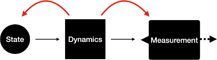
Figure 1: Quantum dynamics can modify static quantum resources either in quantum states or in quantum measurements.

Lastly, quantum dynamics, as a fundamental component of quantum theory alongside quantum states and quantum measurements, plays a more intricate role in the context of quantum resources. First, quantum dynamics can modify static quantum resources in both states and measurements, as illustrated in Fig. 1, encompassing their generation [59, 60, 61, 62, 63], preservation [64], and destruction [65, 66]. In this regard, the conversion of coherence generating power to entanglement-generating power has been demonstrated for quantum dynamics acting on states [67]. Second, static quantum resources can be utilized to implement quantum dynamics [68, 69, 70, 71]. Finally, quantum dynamics itself can serve as a resource, enabling the simulation of other quantum dynamics using operations devoid of quantum resources [72, 73]. In fact, this perspective offers an alternative framing of quantum simulation [74, 75, 76]—one of the most promising applications of quantum computing—emphasizing the interplay between experimental capabilities and the quantum resources required. Despite significant progress, these intricate relations between quantum dynamics and quantum resources are only partially understood.

In this Letter, we complete the coherence-entanglement relation at the dynamics level by establishing the effect of quantum channels on measurement-resources. We develop a resource theory of measurement-resource generating powers for quantum dynamics, building upon existing resource theories of quantum measurements [56]. During our investigation, we reveal that any incoherent measurement is essentially the canonical incoherent basis measurement. We demonstrate that the coherence-entanglement relation is still valid for measurement-resource generating powers of quantum channels. Furthermore, we demonstrate the equivalence between a unital quantum channel’s coherence generating power and its adjoint map’s measurement-coherence generating power, with a weaker relation holding for entanglement. These results reduce to the results on the measurement-resources when quantum measurements are considered as special quantum channels with classical outputs.

Resource theory of measurement-coherence and measurement-entanglement.—In the resource theory of quantum coherence [20], quantum coherence of an operator is quantified with respect to a fixed orthonormal basis, which is referred to as the incoherent basis. The choice of an incoherent basis is contingent upon the experimental or physical constraints imposed on the system under consideration. We set an incoherent basis of a system $A$ and denote it as $\mathcal{I}_{A}=\{\lvert i\rangle_{A}:i=0,\dots,d-1\}$, with respect to which quantum coherence is considered. An operator $O_{A}$ that is diagonal in the incoherent basis is referred to as incoherent. Any incoherent operator is a fixed point under the dephasing channel $\Delta_{A}(O_{A})=\sum_{i=0}^{d-1}\langle i\rvert O_{A}\lvert i\rangle_{A}\left|i\right\rangle\!\left\langle i\right|_{A}=O_{A}$. Similarly, a quantum state $\rho_{A}$ is incoherent if $\Delta_{A}(\rho_{A})=\rho_{A}$. In this paper, we consider constituent systems of dimension $d$ and assume that a quantum measurement for each system would be assumed to have $n$ outcomes, which can be described as a positive operator valued measure (POVM) given by $\mathcal{M}_{A}=\{M_{x}\geq 0:\sum_{x=0}^{n-1}M_{x}=I_{A},x=0,\dots,n-1\}$, where $I_{A}$ is the identity operator. A quantum measurement $\mathcal{M}_{A}$ can be equivalently described by a quantum channel with classical outputs as

$$\mathcal{M}_{A}(\rho_{A})=\sum_{x=0}^{n-1}\operatorname{Tr}_{A}(M_{x}\rho_{A})\left|x\right\rangle\!\left\langle x\right|_{A^{\prime}},$$ (1)

where $\rho_{A}$ is a quantum state and $A^{\prime}$ denotes the output system [77]. The output of a quantum measurement is regarded as being classical implying that $\{\left|x\right\rangle\!\left\langle x\right|_{A^{\prime}}:x=0,\dots,n-1\}$ being an incoherent basis for the system $A^{\prime}$. A quantum measurement $\mathcal{M}_{A}=\{M_{x}\geq 0:\sum_{x=}^{n-1}M_{x}=I_{A},x=0,\dots,n-1\}$ is called an incoherent measurement if its POVM elements are incoherent $\Delta_{A}(M_{x})=M_{x}$ for all $x=0,\dots,n-1$. If a quantum measurement $\mathcal{M}_{A}$ is incoherent, the probability of an outcome is solely dependent on the incoherent information of input states, disregarding the coherent component [53, 78], as demonstrated by the following equation:

$$p(x)=\operatorname{Tr}_{A}M_{x}\rho_{A}=\operatorname{Tr}M_{x}\Delta_{A}(\rho_{A}).$$ (2)

We denote the set of incoherent measurements as $\mathbf{IM}$. Measurement-coherence of a quantum measurement $\mathcal{M}_{A}$ is quantified by the measurement relative entropy of measurement-coherence $C_{m}(\cdot)$, as defined in [56]:

$$C_{m}(\mathcal{M}_{A})=\min_{\mathcal{F}_{A}\in\mathbf{IM}}D_{m}(\mathcal{M}_{A}\|\mathcal{F}_{A}),$$ (3)

where the measurement relative entropy between two quantum measurements $D_{m}(\cdot\|\cdot)$ is proportional to the average relative entropy between POVM elements as

$$D_{m}(\mathcal{M}_{A}\|\mathcal{N}_{A})\coloneqq\dfrac{1}{d}\sum_{x=0}^{n-1}D(M_{x}\|N_{x}),$$ (4)

with the quantum relative entropy $D(\cdot\|\cdot)$. The measurement relative entropy of measurement-coherence of a quantum measurement is found to be equal to the average relative entropy of coherence of each POVM element, up to a multiplicative constant [56]:

$$C_{m}(\mathcal{M}_{A})=\dfrac{1}{d}\sum_{x=0}^{n-1}\{S(\Delta_{A}(M_{x}))-S(M_{x})\},$$ (5)

where $S(X_{A})=-\operatorname{Tr}_{A}X_{A}\log X_{A}$ for $X_{A}\geq 0$ is the von Neumann entropy.

Figure 2: A quantum measurement $\mathcal{M}_{A}$ transforms to another quantum measurement $\widetilde{\mathcal{M}}_{A}$ under a pre-processing channel $\mathcal{E}_{A}$ and a classical processing channel $\mathcal{S}_{A}$. The pre-processing channel can generate measurement-coherence.

A quantum measurement $\mathcal{M}_{A}$ undergoes a transformation into another quantum measurement $\widetilde{\mathcal{M}}_{A}$ when a pre-processing channel is appended and a classical post-processing channel is appended as illustrated in Fig. 2 [49]. This can be described as follows:

$$\widetilde{\mathcal{M}}_{A}=\mathcal{S}_{A^{\prime}}\circ\mathcal{M}_{A}\circ\mathcal{E}_{A},$$ (6)

where a classical post-processing channel $\mathcal{S}_{A^{\prime}}(\rho_{A^{\prime}})=\sum_{x,x^{\prime}=0}^{n-1}p(x^{\prime}|x)\langle x\rvert\rho_{A^{\prime}}\lvert x\rangle_{A^{\prime}}\left|x^{\prime}\right\rangle\!\left\langle x^{\prime}\right|_{A^{\prime}}$ sends an outcome $x$ to another outcome $x^{\prime}$ with a conditional probability distribution $p(x^{\prime}|x)$ satisfying $\sum_{x^{\prime}}p(x^{\prime}|x)=1$ for all $x$. At this point, we demonstrate that an incoherent measurement is, in essence, the incoherent basis measurement:

Theorem 1.

An incoherent measurement $\mathcal{M}_{A}\in\mathbf{IM}$ can be implemented by the incoherent basis measurement $\mathcal{I}_{A}=\{\left|i\right\rangle\!\left\langle i\right|_{A}:i=0,\dots,d-1\}$ followed by a classical post-processing channel $\mathcal{S}_{A}$:

$$\mathcal{M}_{A}=\mathcal{S}_{A}\circ\mathcal{I}_{A}$$ (7)

We defer proofs of the above and subsequent results to the Supplemental Material. The set of quantum channels that do not generate any measurement-coherence is known to be detection-incoherent operations ($\mathbf{DIO}$) [53]. These serve as free operations for measurement-coherence. A quantum channel $\mathcal{E}_{A}$ is in $\mathbf{DIO}$ if and only if it satisfies the equation $\Delta_{A}\circ\mathcal{E}_{A}=\Delta_{A}\circ\mathcal{E}_{A}\circ\Delta_{A}$. This characterization is analogous to the characterization of a quantum channel in the maximal incoherent operations ($\mathbf{MIO}$), which is the largest set of quantum channels that send incoherent states to incoherent states. A quantum channel $\mathcal{E}_{A}$ is in $\mathbf{MIO}$ if it satisfies the equation $\mathcal{E}_{A}\circ\Delta_{A}=\Delta_{A}\circ\mathcal{E}_{A}\circ\Delta_{A}$.

In the resource theory of measurement-entanglement, we take the set of separable measurements ($\mathbf{SepM}$) whose POVMs are separable operators as our free resources. The set of separable channels ($\mathbf{SepC}$) corresponds to the free operations that preserve $\mathbf{SepM}$. Measurement-entanglement of a bipartite quantum measurement $\mathcal{M}_{AB}$ is quantified by the measurement relative entropy of measurement-entanglement of a bipartite quantum measurement $\mathcal{M}_{AB}$ defined as follows [56]:

$$E_{m}(\mathcal{M}_{AB})\coloneqq\min_{\mathcal{F}\in\mathbf{SepM}(A:B)}D_{m}(\mathcal{M}_{AB}\|\mathcal{F}_{AB}).$$ (8)

We remark that, despite the similarities between the resource theories of quantum coherence and entanglement, there is no entanglement-destroying channel that destroys entanglement while holding every separable state as its fixed point [79]. This is in contrast to the case of quantum coherence, where the dephasing channel destroys static quantum coherence while holding every incoherent state as a fixed point of the channel. As a result of this limitation, there is no straightforward operational interpretation or concise formula for $E_{m}$ as there is for the measurement-relative entropy of measurement-coherence reduced in Eq. (5).

Resource theory of measurement-resource generating powers of quantum dynamics.—Now we focus on the capacity of quantum dynamics to generate measurement-resources. Quantum channels are capable of generating measurement-coherence and measurement-entanglement by acting as a pre-processing channel prior to a quantum measurement. In contrast, classical post-processing after a quantum measurement is unable to generate any measurement-resources.

As previously introduced, $\mathbf{DIO}$ is the largest set of quantum channels under which incoherent measurements remain incoherent measurements [56]. In light of this, we define the measurement-coherence generating power of a quantum channel $\mathcal{E}_{A}$ as follows:

$$C(\mathcal{E}_{A})\coloneqq\min_{\mathcal{F}_{A}\in\mathbf{DIO}}\max_{\mathcal{M}_{A\widetilde{A}}\in\mathbf{IM}}D_{m}(\mathcal{M}_{A\widetilde{A}}\circ\mathcal{E}_{A}\|\mathcal{M}_{A\widetilde{A}}\circ\mathcal{F}_{A}),$$ (9)

where the ancillary system $\widetilde{A}$ can be arbitrary. In fact, we find that the measurement-coherence generating power of a quantum channel $\mathcal{E}_{A}$ is equal to the amount of the measurement-coherence generated by the quantum channel $\mathcal{E}_{A}$ from the incoherent basis measurement $\mathcal{I}_{A}$:

Theorem 2.

For a quantum channel $\mathcal{E}_{A}$, the measurement-coherence generating power of the quantum channel is given by

$$C(\mathcal{E}_{A})=C_{m}(\mathcal{I}_{A}\circ\mathcal{E}_{A}),$$ (10)

where $\mathcal{I}_{A}=\{\left|i\right\rangle\!\left\langle i\right|_{A}:i=0,\dots,d-1\}$ is the incoherent-basis measurement.

Similarly, the free resource in measurement-entanglement generating power corresponds to separable channels that send separable operators to themselves in a complete sense [80, 72]. We define the measurement-entanglement generating power of a quantum channel $\mathcal{E}_{AB}$ as follows:

$$E(\mathcal{E}_{AB})\coloneqq\min_{\mathcal{F}\in\mathbf{SepC}(A:B)}\max_{\mathcal{M}\in\mathbf{SepM}(A\widetilde{A}:B\widetilde{B})}\\ D_{m}(\mathcal{M}_{A\widetilde{A}B\widetilde{B}}\circ\mathcal{E}_{AB}\|\mathcal{M}_{A\widetilde{A}B\widetilde{B}}\circ\mathcal{F}_{AB}),$$ (11)

where the ancillary systems $\widetilde{A}$ and $\widetilde{B}$ can be arbitrary. As previously noted, there is no resource-destroying dynamics that fixes any separable state in entanglement theory. Thus, the the aforementioned simplification as in Eq. (10) is not applicable.

The measurement-resource generating powers in Eq. (9) and Eq. (11) are legitimate resource monotones that satisfy the following properties [43]: i) the measurement-coherence generating power $C(\mathcal{E}_{A})$ is non-negative and faithful, that is, $C(\mathcal{E}_{A})$ is zero if and only if $\mathcal{E}_{A}$ is in $\mathbf{DIO}$. ii) The measurement-coherence generating power is monotone under a DIO $\mathcal{K}_{A}$ and a unital $\mathbf{DIO}$ $\mathcal{L}_{A}$ such that $C(\mathcal{K}_{A}\circ\mathcal{E}_{A}\circ\mathcal{L}_{A})\leq C(\mathcal{E}_{A})$. iii) The measurement-coherence generating power is convex, that is, $C(p\mathcal{E}_{A}+(1-p)\mathcal{G}_{A})\leq pC(\mathcal{E}_{A})+(1-p)C(\mathcal{G}_{A})$ for $0\leq p\leq 1$.

Similarly, the measurement-entanglement generating power $E$ also satisfies the three properties: i) $E(\mathcal{E}_{AB})\geq 0$, with equality holding if and only if $\mathcal{E}_{AB}\in\mathbf{SepC}(A\!:\!B)$. ii) The measurement-entanglement generating power $E$ is monotone under the composition by a separable channel $\mathcal{K}_{AB}$ and a unital separable channel $\mathcal{L}_{AB}$ such that $E(\mathcal{K}_{AB}\circ\mathcal{E}_{AB}\circ\mathcal{L}_{AB})\leq E(\mathcal{E}_{AB})$. iii) The measurement-entanglement generating power $E$ is convex, that is, $E(p\mathcal{E}_{AB}+(1-p)\mathcal{G}_{AB})\leq pE(\mathcal{E}_{AB})+(1-p)E(\mathcal{G}_{AB})$ for $0\leq p\leq 1$.

Measurement-coherence generating power conversion to measurement-entanglement generating power.—Having established the concepts of measurement-coherence and measurement-entanglement generating powers of quantum channels, we now present our main result: quantum coherence can be converted to entanglement at the level of dynamics generating measurement resources. First, we demonstrate that the measurement-coherence generating power of a quantum channel $\mathcal{E}_{A}$ serves as an upper bound on the measurement-entanglement generating power of a composite channel constructed using the quantum channel $\mathcal{E}_{A}$, without any additional measurement-coherence generating resources:

Theorem 3.

Let $\mathcal{E}_{A}$ be a quantum channel. Then we have that

$$E(\Delta_{AB}\circ\mathcal{K}_{AB}\circ\mathcal{E}_{A}\circ\mathcal{L}_{AB})\leq C(\mathcal{E}_{A})$$ (12)

for a $\mathbf{DIO}$ channel $\mathcal{K}_{AB}$ and a unital $\mathbf{DIO}$ channel $\mathcal{L}_{AB}$.

Given that the quantum channels surrounding the quantum channel $\mathcal{E}_{A}$ are $\mathbf{DIO}$s, they do not contribute measurement-coherence generating power. Consequently, Theorem 5 implies that measurement-coherence generating power of a quantum channel $\mathcal{E}_{A}$ is the sole source of measurement-entanglement generating power of the composite quantum channel $\widetilde{\mathcal{E}}_{AB}$. Indeed, there exists a configuration that allows for complete conversion of measurement-coherence generating power to measurement-entanglement generating power although we restrict the pre-processing channel $\mathcal{L}_{AB}$ to be unital as the following result shows:

Theorem 4.

For a quantum channel $\mathcal{E}_{A}$, its measurement-coherence generating power can be fully converted to measurement-entanglement generating power under a pre-processing by the adjoint channel of the generalized CNOT channel $\mathcal{U}_{\mathrm{CNOT}}^{{\dagger}}$ and a post-processing dephasing channel:

$$E(\Delta_{AB}\circ\mathcal{E}_{A}\circ\mathcal{U}_{\mathrm{CNOT}}^{{\dagger}})=C(\mathcal{E}_{A}),$$ (13)

where $U_{\mathrm{CNOT}}=\sum_{i,j=0}^{d-1}\left|i,i\oplus j\right\rangle\!\left\langle ij\right|_{AB}$ with $\oplus$ denoting addition modulo $d$.

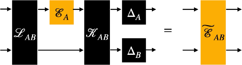
(a)

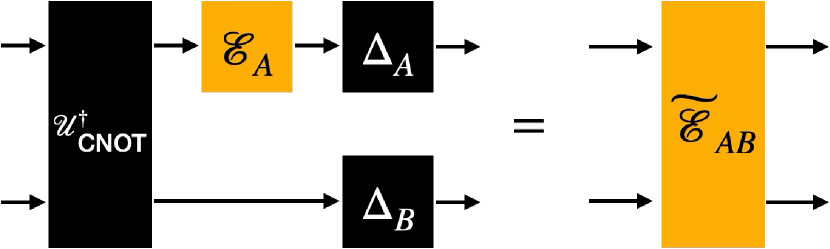
(b)

Figure 3: (a) Measurement-coherence generating power of a quantum channel $\mathcal{E}_{A}$ can convert to measurement-entanglement generating power of a quantum channel $\widetilde{\mathcal{E}}_{AB}$ under a $\mathbf{DIO}$ channel $\mathcal{K}_{AB}$, a unital $\mathbf{DIO}$ channel $\mathcal{L}_{AB}$, and the dephasing channel $\Delta_{AB}$. (b) The optimal conversion can be achieved by employing the adjoint channel of the generalized CNOT channel as a pre-processing channel $\mathcal{L}_{AB}=\mathcal{U}_{\mathrm{CNOT}}^{{\dagger}}$, and the dephasing channel $\Delta_{AB}$ as post-processing.

This result completes the picture of quantum coherence being convertible to quantum entanglement at the dynamic level, specifically by addressing the previously missing element: the conversion of a quantum channel’s measurement-coherence generating power to measurement-entanglement generating power. It is noteworthy that the dephasing channels in this configuration serve to render the subsequent measurement incoherent and align the incoherent basis, thereby enabling the adjoint channel of the generalized CNOT channel to optimally convert the measurement-coherence generating power of the quantum channel $\mathcal{E}_{A}$ into the measurement-entanglement generating power in that incoherent basis.

The convertibility of measurement-coherence generating power to measurement-entanglement generating power implies that a measurement-entanglement generating power monotone induces a measurement-coherence generating power monotone, as demonstrated by the following result:

Theorem 5.

A measurement-entanglement generating power monotone $\widetilde{E}$ induces a measurement-coherence generating power monotone $\widetilde{C}$ given by

$$\widetilde{C}(\mathcal{E}_{A})=\max_{\mathcal{K}_{AB},\mathcal{L}_{AB}}\widetilde{E}(\Delta_{AB}\circ\mathcal{K}_{AB}\circ\mathcal{E}_{A}\cdot\mathcal{L}_{AB}),$$ (14)

where the maximization is over $\mathbf{DIO}$ channels $\mathcal{K}_{AB}$ and unital $\mathbf{DIO}$ channels $\mathcal{L}_{AB}$.

This is the analogous part for the measurement-resource generating powers to a coherence resource monotone induced by an entanglement monotone, as previously demonstrated for static and dynamic resources [45, 67, 56].

Our results reduce to the case of static measurement-resources when considering measurement-resource generating powers for a quantum measurement described as a quantum channel, as in Eq. (1). A quantum measurement $\mathcal{N}_{A}$ is a quantum channel whose output is incoherent, satisfying that $\mathcal{N}_{A}=\Delta_{A}\circ\mathcal{N}_{A}$. This, along with the observation that the dephasing channel corresponds to the incoherent basis measurement, leads to the following result:

Theorem 6.

For a quantum measurement $\mathcal{N}_{A}$ and a bipartite quantum measurement $\mathcal{N}_{AB}$, measurement-coherence generating power and measurement-entanglement generating power reduce to the measurement relative entropy of measurement-coherence and the measurement relative entropy of measurement-entanglement, respectively, as follows:

$$C(\mathcal{N}_{A})=C_{m}(\mathcal{N}_{A}),\quad E(\mathcal{N}_{AB})=E_{m}(\mathcal{N}_{AB}).$$ (15)

We now proceed to investigate the relation between the generating powers of quantum channels with respect to both static quantum resources.

Resource generating power versus measurement-resource generating power.—A quantum channel $\mathcal{E}_{A}$ can generate static quantum resources in both quantum states and measurements. The coherence generating power of a quantum channel $\mathcal{E}_{A}$ is defined as the maximum coherence it can generate from incoherent states:

$$C_{g}(\mathcal{E}_{A})\coloneqq\max_{\sigma_{A\widetilde{A}}\in\mathbf{I}}C_{R}(\mathcal{E}_{A}(\sigma_{A\widetilde{A}})),$$ (16)

where $C_{R}(\rho_{A})\coloneqq\max_{\sigma_{A}\in\mathbf{I}}D(\rho_{A}\|\sigma_{A})$ is the relative entropy of coherence [13], and $\mathbf{I}$ denotes the set of incoherent states.

Are there relations between the two static resource generating powers of a quantum channel? In general, there is no relation between a channel’s resource-generating power and its measurement-resource generating powers. Consider a preparation channel $\mathcal{E}_{A}(\rho_{A})=\operatorname{Tr}_{A}(\rho_{A})\left|+\right\rangle\!\left\langle+\right|_{A}$ for any input state $\rho_{A}$. This quantum channel has the maximum coherence generating power as $C_{g}(\mathcal{E}_{A})=1$ but no measurement-coherence generating power as $C(\mathcal{E}_{A})=0$. Another quantum channel $\mathcal{G}_{A}(\rho_{A})=\langle+\rvert\rho_{A}\lvert+\rangle_{A}\left|0\right\rangle\!\left\langle 0\right|_{A}+\langle-\rvert\rho_{A}\lvert-\rangle_{A}\left|1\right\rangle\!\left\langle 1\right|_{A}$ shows the opposite case where it can generate no quantum coherence as $C_{g}(\mathcal{G}_{A})=0$ while it can generate the maximum measurement-coherence $C(\mathcal{G}_{A})=1$. However, for unital quantum channels, we establish a connection between coherence generation and measurement-coherence generation:

Theorem 7.

For a unital quantum channel $\mathcal{E}_{A}$, the coherence generating power $C_{g}(\mathcal{E}_{A})$ and the measurement-coherence generating power $C(\mathcal{E}_{A}^{{\dagger}})$ of its adjoint channel $\mathcal{E}_{A}^{{\dagger}}$ satisfy the following:

$$\dfrac{1}{d}C_{g}(\mathcal{E}_{A})\leq C(\mathcal{E}_{A}^{{\dagger}})\leq C_{g}(\mathcal{E}_{A}).$$ (17)

This result implies that for a unital quantum channel, the coherence generating power of the channel and the measurement-coherence generating power of its adjoint channel are equivalent in the sense that one is non-zero if and only if the other is non-zero.

For entanglement, we find a weaker relation. The entanglement generating power of a quantum channel $\mathcal{E}_{AB}$ is defined as

$$E_{g}(\mathcal{E}_{AB})\coloneqq\max_{\sigma\in\mathbf{SepD}(A\widetilde{A}:B\widetilde{B})}E_{R}(\mathcal{E}_{AB}(\sigma_{A\widetilde{A}B\widetilde{B}})),$$ (18)

where $E_{R}(\rho_{AB})\coloneqq\min_{\sigma\in\mathbf{SepD}(A:B)}D(\rho_{AB}\|\sigma_{AB})$ is the relative entropy of entanglement [39]. The entanglement generating power of a unital quantum channel upper-bounds the measurement-entanglement generating power of its adjoint channel:

Theorem 8.

For a unital quantum channel $\mathcal{E}_{AB}$, the entanglement-generating power $E_{g}(\mathcal{E}_{AB})$ and the measurement-entanglement generating power $E(\mathcal{E}_{AB}^{{\dagger}})$ of its adjoint channel $\mathcal{E}_{AB}^{{\dagger}}$ satisfy the following:

$$E(\mathcal{E}_{AB}^{{\dagger}})\leq E_{g}(\mathcal{E}_{AB}).$$ (19)

Conclusion.—We have completed the picture of quantum coherence conversion to quantum entanglement across static and dynamic levels as shown in Fig. 4. Our work establishes resource theories for quantum channels’ measurement-coherence and measurement-entanglement generating power, demonstrating that measurement-coherence generating power can be converted to measurement-entanglement generating power. This finding complements the previously known conversions of quantum coherence to quantum entanglement in static resources, such as quantum states and measurements, and the conversion of a quantum channel’s coherence generating power to entanglement generating power. In achieving our main results, we utilized the newly characterized structure of an incoherent measurement as an incoherent basis measurement followed by a classical post-processing channel.

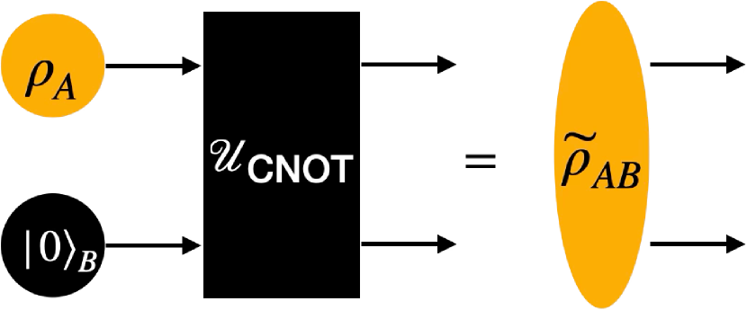
(a) Optimal conversion of quantum coherence of a quantum state $\rho_{A}$ to entanglement of a quantum state $\widetilde{\rho}_{AB}$ [45].

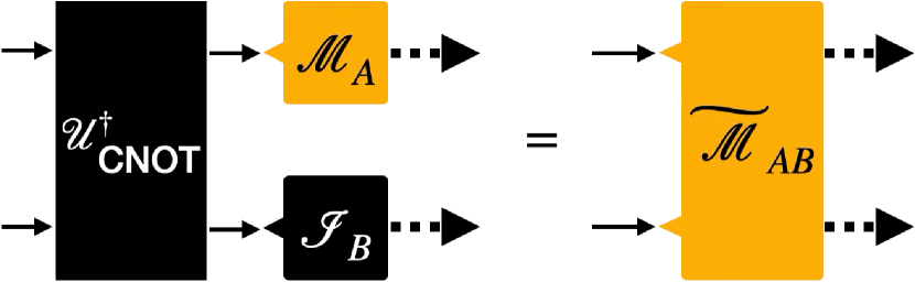
(b) Optimal conversion of measurement-coherence of a quantum measurement $\mathcal{M}_{A}$ to measurement-entanglement of a quantum measurement $\widetilde{\mathcal{M}}_{AB}$ [56].

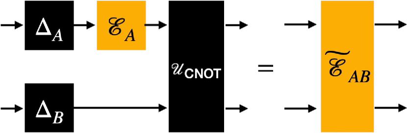
(c) Optimal conversion of coherence generating power of a quantum channel $\mathcal{E}_{A}$ to entanglement generating power of a quantum channel $\widetilde{\mathcal{E}}_{AB}$ [67].

(d) Optimal conversion of measurement-coherence generating power of a quantum channel $\mathcal{E}_{A}$ to measurement-entanglement generating power of a quantum channel $\widetilde{\mathcal{E}}_{AB}$.

Figure 4: Optimal conversion of quantum coherence to entanglement at static and dynamic levels. The left and right columns correspond to the state resource and measurement resource, respectively. The top and bottom rows represent, respectively, static and dynamic resources.

Moreover, we showed that a unital quantum channel’s coherence generating power is essentially equivalent to its adjoint map’s measurement-coherence generating power, while a unital bipartite quantum channel’s entanglement generating power imposes an upper bound on its adjoint channel’s measurement-entanglement generating power. We also present an interpretation of the role of additional dephasing channels in resource-generating power conversion [67] as acting as a pre-processing step to remove incoming static coherence, enabling the conversion of a quantum channel’s static coherence generating power into static entanglement generating power.

Our work encompasses previous findings regarding the conversion of measurement-resources. When a quantum measurement is treated as a quantum channel with classical outputs, our results reproduce the previous results on measurement-coherence and measurement-entanglement.

Despite the significant progress in understanding static and dynamic quantum coherence and entanglement, several open questions remain. While the conversion of quantum coherence to quantum entanglement is well-established, the reverse process remains poorly understood. The primary challenge in this regard is that entanglement does not exhibit a preference for specific bases, making the conversion from entanglement to coherence a non-trivial problem. Moreover, the relation between quantum coherence and multipartite entanglement is still largely unexplored [47], possibly due to the incomplete understanding of multipartite entanglement itself.

Another important aspect to consider is that static resource generating powers do not fully capture all the aspects of quantum dynamics in relation to quantum resources. In fact, quantum dynamics itself can be considered a quantum resource under restricted quantum superchannels [81, 82, 83, 84]. For instance, the generalized Hadamard gate has been studied as a dynamic coherence resource [71], while the SWAP gate has been used as a dynamic entanglement resource to simulate any bipartite quantum channel [73, 84, 85], much like how Bell states can be employed to generate any bipartite quantum state. This problem can be regarded as an instance of quantum simulation with a specific emphasis on quantum resources. However, the relation between these dynamic quantum resources is not as well-understood as the relation between static resource generating powers. A deeper understanding of these dynamic quantum resources could potentially lead to the development of more efficient quantum information processing algorithms, such as quantum simulation.

Addressing these questions will deepen our understanding of the fundamental properties of quantum resources and advance the development of resource-efficient quantum information processing techniques.

I Supplemental material

This supplemental material provides the technical details and proofs for the theorems in the main article. We assume that the systems under consideration have dimension $d$ and that a measurement outputs $n$ outcomes for each system. The symbols $\mathbf{IO}$, $\mathbf{MIO}$, and $\mathbf{DIO}$ are employed to denote the set of incoherent operations, the set of maximally incoherent operations, and the set of detection-incoherent operations, respectively [20]. The set of incoherent measurements is written as $\mathbf{IM}$. For the sake of clarity, the identity channel $\mathsf{id}_{A}$ on a system $A$ is often omitted for clarity.

I.1 Resource theory of measurement-coherence and measurement-entanglement

This section provides a concise overview of the essential elements of measurement-resource theories, primarily developed in [56]: We quantify measurement-resources using the measurement relative entropy $D_{m}(\mathcal{M}_{A}\|\mathcal{N}_{A})$ between measurements $\mathcal{M}_{A}=\{M_{x}\}_{x=0}^{n-1}$ and $\mathcal{N}_{A}=\{N_{x}\}_{x=0}^{n-1}$ defined by

$$D_{m}(\mathcal{M}_{A}\|\mathcal{N}_{A})=\dfrac{1}{d}\sum_{x=0}^{n-1}D(M_{x}\|N_{x}).$$ (20)

Some properties of the measurement relative entropy are as follows:

Lemma 1.

Let $\mathcal{M}_{A},\mathcal{N}_{A},\mathcal{K}_{A},\mathcal{L}_{A}$ be quantum measurements with the output system $A^{\prime}$, $\mathcal{E}_{A}$ a unital quantum channel, and $\mathcal{U}_{A}$ a unitary channel. Let $\mathcal{S}_{A^{\prime}}$ be a classical channel that sends $\lvert x\rangle_{A^{\prime}}$ to $\lvert y\rangle_{A^{\prime}}$ with a probability $p(y|x)$ that satisfies $\sum_{y}p(y|x)=1$ for all $x$. Let $0\leq p\leq 1$. The following holds:

1. $D_{m}(\mathcal{M}_{A}\|\mathcal{N}_{A})\geq 0$; the equality holds if and only if $\mathcal{M}_{A}=\mathcal{N}_{A}$,

2. $D_{m}(\mathcal{M}_{A}\circ\mathcal{E}_{A}\|\mathcal{N}_{A}\circ\mathcal{E}_{A})\leq D_{m}(\mathcal{M}_{A}\|\mathcal{N}_{A}),$

3. $D_{m}(\mathcal{M}_{A}\circ\mathcal{U}_{A}\|\mathcal{N}_{A}\circ\mathcal{U}_{A})=D_{m}(\mathcal{M}_{A}\|\mathcal{N}_{A}),$

4. $D_{m}(\mathcal{S}_{A^{\prime}}\circ\mathcal{M}_{A}\|\mathcal{S}_{A^{\prime}}\circ\mathcal{N}_{A})\leq D_{m}(\mathcal{M}_{A}\|\mathcal{N}_{A})$,

5. $D_{m}(\mathcal{M}_{A}\otimes\mathcal{N}_{B}\|\mathcal{K}_{A}\otimes\mathcal{L}_{B})=D_{m}(\mathcal{M}_{A}\|\mathcal{K}_{A})+D_{m}(\mathcal{N}_{B}\|\mathcal{L}_{B}),$

6. $D_{m}(p\mathcal{M}_{A}+(1-p)\mathcal{N}_{A}\|p\mathcal{K}_{A}+(1-p)\mathcal{L}_{A})\leq pD_{m}(\mathcal{M}_{A}\|\mathcal{K}_{A})+(1-p)D_{m}(\mathcal{N}_{A}\|\mathcal{L}_{A}).$

In measurement-coherence resource theory, the set of incoherent measurements ($\mathbf{IM}$) is the free resource and the detection-incoherent operations ($\mathbf{DIO}$) with classical post-processing channels correspond to the free operations that do not generate any measurement-coherence from incoherent measurements. The measurement-coherence of a measurement $\mathcal{M}_{A}=\{M_{x}\}$ is quantified by the measurement relative entropy of measurement-coherence defined as

$$C_{m}(\mathcal{M}_{A}) \coloneqq\min_{\mathcal{F}_{A}\in\mathbf{IM}}D_{m}(\mathcal{M}_{A}\|\mathcal{F}_{A})$$ (21)

$$=\dfrac{1}{d}\sum_{x=0}^{n-1}\{S(\Delta(M_{x}))-S(M_{x})\},$$ (22)

where $S(X_{A})=-\operatorname{Tr}_{A}X_{A}\log X_{A}$ for $X_{A}\geq 0$ is the von Neumann entropy. In measurement-entanglement resource theory, the set of separable measurement ($\mathbf{SepM}$) is the free resources and the set of separable channels ($\mathbf{SepC}$) with classical post-processing channels does the role of free operations. The measurement-entanglement is quantified by the measurement relative entropy of measurement-entanglement defined as

$$E_{m}(\mathcal{M}_{AB})\coloneqq\min_{\mathcal{F}\in\mathbf{SepM}(A\!:\!B)}D_{m}(\mathcal{M}_{AB}\|\mathcal{F}_{AB}).$$ (23)

We demonstrate that an incoherent measurement is the incoherent basis measurement followed by a classical post-processing channel. It employs the observation that the dephasing channel can be seen as the incoherent basis measurement as below:

Proposition 1.

The dephasing channel $\Delta_{A}$ with respect to the incoherent basis $\mathcal{I}_{A}=\{\lvert i\rangle_{A}:i=0,\dots,d-1\}$ is equivalent to the quantum measurement in the incoherent basis $\mathcal{I}_{A}$ as a quantum channel, that is, $\mathcal{I}_{A}(\rho_{A})=\sum_{i=0}^{d-1}\operatorname{Tr}_{A}(\left|i\right\rangle\!\left\langle i\right|_{A}\rho_{A})\left|i\right\rangle\!\left\langle i\right|_{A}$.

Lemma 2 (Structure of an incoherent measurement).

An incoherent measurement $\mathcal{M}_{A}=\{M_{x}\}_{x=0}^{n-1}\in\mathbf{IM}$ is equivalent to an incoherent basis measurement $\mathcal{I}_{A}=\{\left|i\right\rangle\!\left\langle i\right|_{A}:i=0,\dots,d-1\}$ followed by a classical post-processing channel represented as $\mathcal{S}_{A}\circ\mathcal{I}_{A}$, where

$$\mathcal{S}_{A}(X_{A})=\sum_{x,i}p(x|i)\operatorname{Tr}_{A}\left(\left|i\right\rangle\!\left\langle i\right|_{A}X_{A}\right)\left|x\right\rangle\!\left\langle x\right|_{A^{\prime}}$$ (24)

with a conditional probability distribution $p(x|i)=\langle i\rvert M_{x}\lvert i\rangle_{A}\geq 0$ satisfying $\sum_{x}p(x|i)=1$ for all $i$ is a classical post-processing channel.

Proof.

We employ Proposition 1 that the dephasing channel $\Delta_{A}$ is equivalent to the quantum measurement in the incoherent basis $\mathcal{I}_{A}$:

$$\mathcal{M}_{A}(\mathcal{\rho_{A}}) =\mathcal{M}_{A}\circ\Delta_{A}(\rho_{A})$$ (25)

$$=\mathcal{M}_{A}\circ\mathcal{I}_{A}(\rho_{A})$$ (26)

$$=\sum_{i}\operatorname{Tr}_{A}(\left|i\right\rangle\!\left\langle i\right|_{A}\rho_{A})\mathcal{M}_{A}(\left|i\right\rangle\!\left\langle i\right|_{A})$$ (27)

$$=\sum_{i}\operatorname{Tr}_{A}(\left|i\right\rangle\!\left\langle i\right|_{A}\rho_{A})\sum_{x}\operatorname{Tr}_{A}(M_{x}\left|i\right\rangle\!\left\langle i\right|_{A})\left|x\right\rangle\!\left\langle x\right|_{A^{\prime}}$$ (28)

$$=\sum_{x}\sum_{i}p(x|i)\operatorname{Tr}_{A}(\left|i\right\rangle\!\left\langle i\right|_{A}\rho_{A})\left|x\right\rangle\!\left\langle x\right|_{A^{\prime}}$$ (29)

$$=\mathcal{S}_{A}\circ\mathcal{I}_{A}(\rho_{A}).$$ (30)

$\mathcal{M}_{A}$ is a POVM, hence it holds that $p(x|i)=\langle i\rvert M_{x}\lvert i\rangle_{A}\geq 0$ and $\sum_{x}p(x|i)=1$ for all $i$. ∎

Corollary 2.

A bipartite incoherent measurement $\mathcal{M}_{AB}\in\mathbf{IM}$ is equal to the incoherent basis measurement $\mathcal{I}_{AB}=\{\left|ij\right\rangle\!\left\langle ij\right|_{AB}:i,j=0,\dots,d-1\}$ followed by a classical post-processing channel $\mathcal{S}_{AB}\circ\mathcal{I}_{AB}$, where $\mathcal{S}_{AB}(X_{AB})=\sum_{x,y,i,j}p(x,y|i,j)\operatorname{Tr}_{AB}(\left|ij\right\rangle\!\left\langle ij\right|_{AB}X_{AB})\left|xy\right\rangle\!\left\langle xy\right|_{A^{\prime}B^{\prime}}$ with a conditional probability distribution $p(x,y|i,j)=\langle i,j\rvert M_{xy}\lvert ij\rangle_{AB}$ is a classical post-processing channel.

Proof.

A similar calculation as in Lemma 2 shows the result. ∎

Note that Lemma 2 and Corollary 2 hold for any measurement $\mathcal{M}$ with an arbitrary number of measurement outcomes.

I.2 Resource theory of measurement-resource generating powers

I.2.1 Measurement-coherence generating power

The free static resource regarding measurement-coherence is the set of incoherent measurements $\mathbf{IM}$, and the largest set of the free operations is $\mathbf{DIO}$. We define the measurement-coherence generating power of a quantum channel as below:

Definition 1.

The measurement-coherence generating power of a quantum channel $\mathcal{E}_{A}$ is defined as

$$C(\mathcal{E}_{A})\coloneqq\min_{\mathcal{F}_{A}\in\mathbf{DIO}}\max_{\mathcal{M}_{A\widetilde{A}}\in\mathbf{IM}}D_{m}(\mathcal{M}_{A\widetilde{A}}\circ\mathcal{E}_{A}\|\mathcal{M}_{A\widetilde{A}}\circ\mathcal{F}_{A}),$$ (31)

where the maximization is over $\mathbf{IM}$ with an arbitrary ancillary system $\widetilde{A}$.

The following lemma demonstrates that the optimizations in the definition of the measurement-coherence generating power are unnecessary:

Lemma 3.

The measurement-coherence generating power of a quantum channel $\mathcal{E}_{A}$ is equal to the maximum measurement-coherence that can be generated via the quantum channel $\mathcal{E}_{A}$ from incoherent measurements. Furthermore, it is equal to the measurement relative entropy of measurement-coherence of the incoherent basis measurement $\mathcal{I}_{A}=\{\left|i\right\rangle\!\left\langle i\right|_{A}:i=0,\dots,d-1\}$ with the pre-processing channel $\mathcal{E}_{A}$:

$$C(\mathcal{E}_{A})=\max_{\mathcal{M}_{A}\in\mathbf{IM}}C_{m}(\mathcal{M}_{A}\circ\mathcal{E}_{A})=C_{m}(\mathcal{I}_{A}\circ\mathcal{E}_{A}).$$ (32)

For the proof of Lemma 3, we need the following result:

Lemma 4.

For quantum channels $\mathcal{E}_{A}$ and $\mathcal{F}_{A}$, it holds that

$$\max_{\mathcal{M}_{A\widetilde{A}}\in\mathbf{IM}}D_{m}(\mathcal{M}_{A\widetilde{A}}\circ\mathcal{E}_{A}\|\mathcal{M}_{A\widetilde{A}}\circ\mathcal{F}_{A})=\max_{\mathcal{M}_{A}\in\mathbf{IM}}D_{m}(\mathcal{M}_{A}\circ\mathcal{E}_{A}\|\mathcal{M}_{A}\circ\mathcal{F}_{A}),$$ (33)

where the ancillary system $\widetilde{A}$ can be arbitrary.

Proof.

The left-hand side (LHS) is equal to or greater than the right-hand side (RHS) due to the broader domain being considered for maximization. The opposite direction is demonstrated below by employing the structure of a bipartite incoherent measurement as stated in Corollary 2. Denoting the set of classical post-processing channels as $\mathbf{S}$, it follows that

$$\max_{\mathcal{M}_{A\widetilde{A}}\in\mathbf{IM}}D_{m}(\mathcal{M}_{A\widetilde{A}}\circ\mathcal{E}_{A}\|\mathcal{M}_{A\widetilde{A}}\circ\mathcal{F}_{A}) =\max_{\mathcal{S}_{A\widetilde{A}}\in\mathbf{S}}D_{m}(\mathcal{S}_{A\widetilde{A}}\circ\mathcal{I}_{A\widetilde{A}}\circ\mathcal{E}_{A}\|\mathcal{S}_{A\widetilde{A}}\circ\mathcal{I}_{A\widetilde{A}}\circ\mathcal{F}_{A})$$ (34)

$$\leq D_{m}(\mathcal{I}_{A\widetilde{A}}\circ\mathcal{E}_{A}\|\mathcal{I}_{A\widetilde{A}}\circ\mathcal{F}_{A})$$ (35)

$$=D_{m}(\mathcal{I}_{A}\circ\mathcal{E}_{A}\|\mathcal{I}_{A}\circ\mathcal{F}_{A})$$ (36)

$$\leq\max_{\mathcal{M}_{A}\in\mathbf{IM}}D_{m}(\mathcal{M}_{A}\circ\mathcal{E}_{A}\|\mathcal{M}_{A}\circ\mathcal{F}_{A}),$$ (37)

where the first inequality follows from the monotonicity of $D_{m}$ under classical post-processing channels. ∎

Here’s the proof of Lemma 3:

Proof.

A quantum channel $\mathcal{F}_{A}$ is $\mathbf{DIO}$ if $\mathcal{F}_{A}^{{\dagger}}\circ\Delta_{A}=\Delta_{A}\circ\mathcal{F}_{A}^{{\dagger}}\circ\Delta_{A}$. The measurement-coherence generating power of a quantum channel $\mathcal{E}_{A}$ is given by

$$C(\mathcal{E}_{A}) \coloneqq\min_{\mathcal{F}_{A}\in\mathbf{DIO}}\max_{\mathcal{M}_{A\widetilde{A}}\in\mathbf{IM}}D_{m}(\mathcal{M}_{A\widetilde{A}}\circ\mathcal{E}_{A}\|\mathcal{M}_{A\widetilde{A}}\circ\mathcal{F}_{A})$$ (38)

$$=\min_{\mathcal{F}_{A}\in\mathbf{DIO}}\max_{\mathcal{M}_{A}\in\mathbf{IM}}D_{m}(\mathcal{M}_{A}\circ\mathcal{E}_{A}\|\mathcal{M}_{A}\circ\mathcal{F}_{A})$$ (39)

$$=\min_{\mathcal{F}_{A}\in\mathbf{DIO}}\max_{\mathcal{M}_{A}\in\mathbf{IM}}\dfrac{1}{d}\sum_{x}D(\mathcal{E}_{A}^{{\dagger}}(M^{x}_{A})\|\mathcal{F}_{A}^{{\dagger}}(M^{x}_{A})),$$ (40)

where we used Lemma 4 for the second equality. For $\mathcal{M}_{A}\in\mathbf{IM}$, we have that $\mathcal{F}_{A}^{{\dagger}}(M^{x}_{A})=\mathcal{F}_{A}^{{\dagger}}\circ\Delta_{A}(M^{x}_{A})=\Delta_{A}\circ\mathcal{F}_{A}^{{\dagger}}(M^{x}_{A})$. Using $D(X\|\Delta(Y))=S(\Delta(X))-S(X)+D(\Delta(X)\|\Delta(Y))$, we find that

$$C(\mathcal{E}_{A}) =\min_{\mathcal{F}_{A}\in\mathbf{DIO}}\max_{\mathcal{M}_{A}\in\mathbf{IM}}\dfrac{1}{d}\sum_{x}\{S(\Delta_{A}\circ\mathcal{E}_{A}^{{\dagger}}(M^{x}_{A}))-S(\mathcal{E}_{A}^{{\dagger}}(M^{x}_{A}))$$ (41)

$$\qquad+D(\Delta_{A}\circ\mathcal{E}_{A}^{{\dagger}}(M^{x}_{A})\|\Delta_{A}\circ\mathcal{F}_{A}^{{\dagger}}(M^{x}_{A}))\}$$ (42)

$$=\max_{\mathcal{M}_{A}\in\mathbf{IM}}\dfrac{1}{d}\sum_{x}\left\{S(\Delta_{A}\circ\mathcal{E}_{A}^{{\dagger}}(M^{x}_{A}))-S(\mathcal{E}_{A}^{{\dagger}}(M^{x}_{A}))\right\}$$ (43)

$$=\max_{\mathcal{M}_{A}\in\mathbf{IM}}C_{m}(\mathcal{M}_{A}\circ\mathcal{E}_{A})$$ (44)

$$=\max_{\mathcal{S}_{A}\in\mathbf{S}}C_{m}(\mathcal{S}_{A}\circ\mathcal{I}_{A}\circ\mathcal{E}_{A})$$ (45)

$$=C_{m}(\mathcal{I}_{A}\circ\mathcal{E}_{A}),$$ (46)

where we choose $\mathcal{F}_{A}=\mathcal{E}_{A}\circ\Delta_{A}\in\mathbf{DIO}$ in the second equality regarding the non-negativity of the relative entropy. The fourth equality follows from Lemma 2, and the final equality holds from the monotonicity of $C_{m}$ under classical post-processing channels. ∎

Theorem 3.

The measurement-coherence generating power $C(\mathcal{E}_{A})$ of a quantum channel $\mathcal{E}_{A}$ is a resource monotone satisfying

1. Non-negativity and faithfulness: $C(\mathcal{E}_{A})\geq 0$. $C(\mathcal{E}_{A})=0$ if and only if $\mathcal{E}_{A}\in\mathbf{DIO}$.

2. Monotonicity: For a detection-incoherent channel $\mathcal{K}_{A}$ and a unital detection-incoherent channel $\mathcal{L}_{A}$, it holds that

   $$C(\mathcal{K}_{A}\circ\mathcal{E}_{A}\circ\mathcal{L}_{A})\leq C(\mathcal{E}_{A}).$$ (47)

3. Convexity: For quantum channels $\mathcal{E}_{A}$ and $\mathcal{G}_{A}$, it holds that $C(p\mathcal{E}_{A}+(1-p)\mathcal{G}_{A})\leq pC(\mathcal{E}_{A})+(1-p)C(\mathcal{G}_{A})$ for $0\leq p\leq 1$.

Proof.

1. Non-negativity and faithfulness can be shown as follows: $C(\mathcal{E}_{A})\geq 0$ due to the non-negativity of $D_{m}$. $C(\mathcal{E}_{A})=0$ for $\mathcal{E}_{A}\in\mathbf{DIO}$ from the definition. If $\mathcal{E}_{A}\notin\mathbf{DIO}$, there exists $\mathcal{M}_{A\widetilde{A}}\in\mathbf{IM}$ such that $\mathcal{M}_{A\widetilde{A}}\circ\mathcal{E}_{A}\notin\mathbf{IM}$ implying $C(\mathcal{E}_{A})>0$ since $\mathbf{DIO}$ is the largest set that preserves $\mathbf{IM}$. Therefore, it holds that $C(\mathcal{E}_{A})=0$ if and only if $\mathcal{E}_{A}\in\mathbf{DIO}$.

2. For a detection-incoherent channel $\mathcal{K}_{A}$ and a unital detection-incoherent channel $\mathcal{L}_{A}$, it follows that

   $$C(\mathcal{K}_{A}\circ\mathcal{E}_{A}\circ\mathcal{L}_{A}) =\max_{\mathcal{M}_{A}\in\mathbf{IM}}C_{m}(\mathcal{M}_{A}\circ\mathcal{K}_{A}\circ\mathcal{E}_{A}\circ\mathcal{L}_{A})$$ (48)

   $$\leq\max_{\mathcal{M}_{A}\in\mathbf{IM}}C_{m}(\mathcal{M}_{A}\circ\mathcal{E}_{A}\circ\mathcal{L}_{A})$$ (49)

   $$\leq\max_{\mathcal{M}_{A}\in\mathbf{IM}}C_{m}(\mathcal{M}_{A}\circ\mathcal{E}_{A})$$ (50)

   $$=C(\mathcal{E}_{A}),$$ (51)

   where the first inequality follows due to $\mathcal{M}_{A}\circ\mathcal{K}_{A}\in\mathbf{IM}$, and the second inequality holds from the monotonicity of $C_{m}$ under unital detection-incoherent channels. The last equality is given by Lemma 3.

3. Convexity follows from the convexity of $C_{m}$ and Lemma 3: We first show that $C_{m}$ is convex: for a set of quantum measurements $\{\mathcal{M}_{i}\}$, let $C_{m}(\mathcal{M}_{i})=D_{m}(\mathcal{M}_{i}\|\mathcal{F}_{i}^{\ast})$ for an incoherent measurement $\mathcal{F}_{i}^{\ast}$. Then, we have that, for a probability vector $\vec{p}$ satisfying $\sum_{i}p_{i}=1$, it follows that

   $$C_{m}\left(\sum_{i}p_{i}\mathcal{M}_{i}\right) =\min_{\mathcal{F}\in\mathbf{IM}}D_{m}\left(\sum_{i}p_{i}\mathcal{M}_{i}\|\mathcal{F}\right)$$ (52)

   $$\leq D_{m}\left(\sum_{i}p_{i}\mathcal{M}_{i}\|\sum_{i}p_{i}\mathcal{F}_{i}^{\ast}\right)$$ (53)

   $$\leq\sum_{i}p_{i}D_{m}\left(\mathcal{M}_{i}\|\mathcal{F}_{i}^{\ast}\right)$$ (54)

   $$=\sum_{i}p_{i}C_{m}(\mathcal{M}_{i}),$$ (55)

   where the second inequality follows from the joint convexity of the measurement relative entropy $D_{m}$. Now Lemma 3 and convexity of $C_{m}$ imply that

   $$C(p\mathcal{E}_{A}+(1-p)\mathcal{G}_{A}) =C_{m}(\mathcal{I}_{A}\circ(p\mathcal{E}_{A}+(1-p)\mathcal{G}_{A}))$$ (56)

   $$\leq pC_{m}(\mathcal{I}_{A}\circ\mathcal{E}_{A})+(1-p)C_{m}(\mathcal{I}_{A}\circ\mathcal{G}_{A})$$ (57)

   $$\leq pC(\mathcal{E}_{A})+(1-p)C(\mathcal{G}_{A}).$$ (58)

∎

I.2.2 Measurement-entanglement generating power

For measurement-entanglement, the free static resource is the set of separable measurements ($\mathbf{SepM}$). Taking free dynamic resource as the set of separable channels ($\mathbf{SepC}$), we define the measurement-entanglement generating power of a quantum channel as follows:

Definition 2.

The measurement-entanglement generating power of a quantum channel $\mathcal{E}_{AB}$ is defined as

$$E(\mathcal{E}_{AB})\coloneqq\min_{\mathcal{F}\in\mathbf{SepC}(A\!:\!B)}\max_{\mathcal{M}\in\mathbf{SepM}(A\widetilde{A}\!:\!B\widetilde{B})}D_{m}(\mathcal{M}_{A\widetilde{A}B\widetilde{B}}\circ\mathcal{E}_{AB}\|\mathcal{M}_{A\widetilde{A}B\widetilde{B}}\circ\mathcal{F}_{AB}),$$ (59)

where the ancillary systems $\widetilde{A}$ and $\widetilde{B}$ can be arbitrary.

There is no preferred basis for entanglement, which is the cause of lack of simplified expression like Lemma 3 for the measurement-coherence generating power.

Theorem 4.

The measurement-entanglement generating power of a quantum channel $\mathcal{E}_{A}$ is a resource monotone satisfying

1. Non-negativity and faithfulness: $E(\mathcal{E}_{AB}\geq 0)$. $E(\mathcal{E}_{AB})=0$ if and only if $\mathcal{E}_{AB}\in\mathbf{SepC}(A\!:\!B)$.

2. Monotonicity: For a separable channel $\mathcal{K}_{AB}$ and a unital separable channel $\mathcal{L}_{AB}$, it follows that

   $$E(\mathcal{K}_{AB}\circ\mathcal{E}_{AB}\circ\mathcal{L}_{AB})\leq E(\mathcal{E}_{AB}).$$ (60)

3. Convexity: For quantum channels $\mathcal{E}_{AB}$ and $\mathcal{G}_{AB}$, it holds that $E(p\mathcal{E}_{AB}+(1-p)\mathcal{G}_{AB})\leq pE(\mathcal{E}_{AB})+(1-p)E(\mathcal{G}_{AB})$ for $0\leq p\leq 1$.

Proof.

1. Non-negativity and faithfulness can be shown as follows: $E(\mathcal{E}_{AB})\geq 0$ due to the non-negativity of $D_{m}$. $E(\mathcal{E}_{AB})=0$ for $\mathcal{E}_{AB}\in\mathbf{SepC}(A\!:\!B)$ from the definition. If $\mathcal{E}_{AB}\notin\mathbf{SepC}(A\!:\!B)$, there exists $\mathcal{M}_{A\widetilde{A}B\widetilde{B}}\in\mathbf{SepM}(A\widetilde{A}\!:\!B\widetilde{B})$ such that $\mathcal{M}_{A\widetilde{A}B\widetilde{B}}\circ\mathcal{E}_{AB}\notin\mathbf{SepM}(A\widetilde{A}\!:\!B\widetilde{B})$ since $\mathbf{SepC}(A\!:\!B)$ is the largest set that preserves $\mathbf{SepM}(A\widetilde{A}\!:\!B\widetilde{B})$ even when acting on subsystems. Therefore, it holds that $E(\mathcal{E}_{AB})=0$ if and only if $\mathcal{E}_{AB}\in\mathbf{SepC}(A\!:\!B)$.

2. For a separable channel $\mathcal{K}_{AB}$ and a unital separable channel $\mathcal{L}_{AB}$, it follows that

   $$E(\mathcal{K}_{AB}\circ\mathcal{E}_{AB}\circ\mathcal{L}_{AB}) =\min_{\mathcal{F}\in\mathbf{SepC}(A\!:\!B)}\max_{\mathcal{M}\in\mathbf{SepM}(A\widetilde{A}\!:\!B\widetilde{B})}$$ (61)

   $$\qquad D_{m}(\mathcal{M}_{A\widetilde{A}B\widetilde{B}}\circ\mathcal{K}_{AB}\circ\mathcal{E}_{AB}\circ\mathcal{L}_{AB}\|\mathcal{M}_{A\widetilde{A}B\widetilde{B}}\circ\mathcal{F}_{AB})$$ (62)

   $$\leq\min_{\mathcal{F}\in\mathbf{SepC}(A\!:\!B)}\max_{\mathcal{M}\in\mathbf{SepM}(A\widetilde{A}\!:\!B\widetilde{B})}$$ (63)

   $$\qquad D_{m}(\mathcal{M}_{A\widetilde{A}B\widetilde{B}}\circ\mathcal{K}_{AB}\circ\mathcal{E}_{AB}\circ\mathcal{L}_{AB}\|\mathcal{M}_{A\widetilde{A}B\widetilde{B}}\circ\mathcal{K}_{AB}\circ\mathcal{F}_{AB}\circ\mathcal{L}_{AB})$$ (64)

   $$\leq\min_{\mathcal{F}\in\mathbf{SepC}(A\!:\!B)}\max_{\mathcal{M}\in\mathbf{SepM}(A\widetilde{A}\!:\!B\widetilde{B})}$$ (65)

   $$\qquad D_{m}(\mathcal{M}_{A\widetilde{A}B\widetilde{B}}\circ\mathcal{K}_{AB}\circ\mathcal{E}_{AB}\|\mathcal{M}_{A\widetilde{A}B\widetilde{B}}\circ\mathcal{K}_{AB}\circ\mathcal{F}_{AB})$$ (66)

   $$\leq\min_{\mathcal{F}\in\mathbf{SepC}(A\!:\!B)}\max_{\mathcal{M}\in\mathbf{SepM}(A\widetilde{A}\!:\!B\widetilde{B})}$$ (67)

   $$\qquad D_{m}(\mathcal{M}_{A\widetilde{A}B\widetilde{B}}\circ\mathcal{E}_{AB}\|\mathcal{M}_{A\widetilde{A}B\widetilde{B}}\circ\mathcal{F}_{AB})$$ (68)

   $$=E(\mathcal{E}_{AB}),$$ (69)

   where the first inequality follows because $\mathcal{K}_{AB}\circ\mathcal{F}_{AB}\circ\mathcal{L}_{AB}\in\mathbf{SepC}(A\!:\!B)$, the second inequality holds from the monotonicity of $D_{m}$, and the third inequality is due to $\mathcal{M}_{A\widetilde{A}B\widetilde{B}}\circ\mathcal{K}_{AB}\in\mathbf{SepM}(A\widetilde{A}\!:\!B\widetilde{B})$.

3. Convexity:

   $$E(p\mathcal{E}_{AB}+(1-p)\mathcal{G}_{AB}) =\min_{\mathcal{F}\in\mathbf{SepC}(A\!:\!B)}\max_{\mathcal{M}\in\mathbf{SepM}(A\widetilde{A}\!:\!B\widetilde{B})}$$ (70)

   $$\qquad D_{m}(\mathcal{M}_{A\widetilde{A}B\widetilde{B}}\circ\{p\mathcal{E}_{AB}+(1-p)\mathcal{G}_{AB}\}\|\mathcal{M}_{A\widetilde{A}B\widetilde{B}}\circ\mathcal{F}_{AB})$$ (71)

   $$=\min_{\mathcal{F},\mathcal{F}^{\prime}\in\mathbf{SepC}(A\!:\!B)}\max_{\mathcal{M}\in\mathbf{SepM}(A\widetilde{A}\!:\!B\widetilde{B})}$$ (72)

   $$\qquad D_{m}(\mathcal{M}_{A\widetilde{A}B\widetilde{B}}\circ\{p\mathcal{E}_{AB}+(1-p)\mathcal{G}_{AB}\}\|$$ (73)

   $$\qquad\qquad\mathcal{M}_{A\widetilde{A}B\widetilde{B}}\circ\{p\mathcal{F}_{AB}+(1-p)\mathcal{F^{\prime}}_{AB})$$ (74)

   $$\leq\min_{\mathcal{F},\mathcal{F}^{\prime}\in\mathbf{SepC}(A\!:\!B)}\max_{\mathcal{M}\in\mathbf{SepM}(A\widetilde{A}\!:\!B\widetilde{B})}$$ (75)

   $$\qquad\{pD_{m}(\mathcal{M}_{A\widetilde{A}B\widetilde{B}}\circ\mathcal{E}_{AB}\|\mathcal{M}_{A\widetilde{A}B\widetilde{B}}\circ\mathcal{F}_{AB})$$ (76)

   $$\qquad+(1-p)D_{m}(\mathcal{M}_{A\widetilde{A}B\widetilde{B}}\circ\mathcal{G}_{AB}\|\mathcal{M}_{A\widetilde{A}B\widetilde{B}}\circ\mathcal{F^{\prime}}_{AB})\}$$ (77)

   $$\leq\min_{\mathcal{F},\mathcal{F}^{\prime}\in\mathbf{SepC}(A\!:\!B)}$$ (78)

   $$\quad\bigg{\{}\max_{\mathcal{M}\in\mathbf{SepM}(A\widetilde{A}\!:\!B\widetilde{B})}pD_{m}(\mathcal{M}_{A\widetilde{A}B\widetilde{B}}\circ\mathcal{E}_{AB}\|\mathcal{M}_{A\widetilde{A}B\widetilde{B}}\circ\mathcal{F}_{AB})$$ (79)

   $$\quad+\max_{\mathcal{M}^{\prime}\in\mathbf{SepM}(A\widetilde{A}\!:\!B\widetilde{B})}(1-p)D_{m}(\mathcal{M}_{A\widetilde{A}B\widetilde{B}}^{\prime}\circ\mathcal{G}_{AB}\|\mathcal{M}_{A\widetilde{A}B\widetilde{B}}^{\prime}\circ\mathcal{F^{\prime}}_{AB})\bigg{\}}$$ (80)

   $$=pE(\mathcal{E}_{AB})+(1-p)E(\mathcal{G}_{AB}),$$ (81)

   where the joint convexity of $D_{m}$ is used for the first inequality.

∎

I.2.3 Main results

Measurement-coherence generating power conversion to measurement-entanglement generating power

Here we demonstrate our main results that the measurement-coherence generating power of a quantum channel can be converted to the measurement-entanglement generating power in composition with free channels. The following lemma will be used to prove the main results:

Lemma 5.

For quantum channels $\mathcal{E}_{AB}$ and $\mathcal{F}_{AB}$, it holds that

$$\max_{\mathcal{M}\in\mathbf{SepM}(A\widetilde{A}\!:\!B\widetilde{B})} D_{m}(\mathcal{M}_{A\widetilde{A}B\widetilde{B}}\circ\Delta_{AB}\circ\mathcal{E}_{AB}\|\mathcal{M}_{A\widetilde{A}B\widetilde{B}}\circ\Delta_{AB}\circ\mathcal{F}_{AB})$$

$$=\max_{\mathcal{M}\in\mathbf{SepM}(A\!:\!B)}D_{m}(\mathcal{M}_{AB}\circ\Delta_{AB}\circ\mathcal{E}_{AB}\|\mathcal{M}_{AB}\circ\Delta_{AB}\circ\mathcal{F}_{AB})$$ (82)

Proof.

The left-hand side (LHS) is equal to or greater than the right-hand side (RHS) due to the broader domain being considered for maximization. The opposite direction is demonstrated below:

$$\max_{\mathcal{M}\in\mathbf{SepM}(A\widetilde{A}:B\widetilde{B})}D_{m}(\mathcal{M}_{A\widetilde{A}B\widetilde{B}}\circ\Delta_{AB}\circ\mathcal{E}_{AB}\|\mathcal{M}_{A\widetilde{A}B\widetilde{B}}\circ\Delta_{AB}\circ\mathcal{F}_{AB})$$ (83)

$$=\max_{\mathcal{M}\in\mathbf{SepM}(A\widetilde{A}:B\widetilde{B})}\dfrac{1}{d^{4}}\sum_{x}D(\mathcal{E}_{AB}^{{\dagger}}\circ\Delta_{AB}(M_{A\widetilde{A}B\widetilde{B}}^{x})\|\mathcal{F}_{AB}^{{\dagger}}\circ\Delta_{AB}(M_{A\widetilde{A}B\widetilde{B}}^{x}))$$ (84)

$$=\max_{\mathcal{M}\in\mathbf{SepM}(A\widetilde{A}:B\widetilde{B})}\dfrac{1}{d^{4}}\sum_{x}D\bigg{(}\sum_{i,j}\mathcal{E}_{AB}^{{\dagger}}(\left|ij\right\rangle\!\left\langle ij\right|_{AB})\otimes\langle ij\rvert M_{A\widetilde{A}B\widetilde{B}}^{x}\lvert ij\rangle_{AB}\bigg{\|}$$ (85)

$$\qquad\qquad\qquad\qquad\quad\sum_{i,j}\mathcal{F}_{AB}^{{\dagger}}(\left|ij\right\rangle\!\left\langle ij\right|_{AB})\otimes\langle ij\rvert M_{A\widetilde{A}B\widetilde{B}}^{x}\lvert ij\rangle_{AB}\bigg{)}$$ (86)

$$\leq\max_{\mathcal{M}\in\mathbf{SepM}(A\widetilde{A}:B\widetilde{B})}\dfrac{1}{d^{4}}\sum_{x}\sum_{i,j}\operatorname{Tr}_{\widetilde{A}\widetilde{B}}(\langle ij\rvert M_{A\widetilde{A}B\widetilde{B}}^{x}\lvert ij\rangle_{AB})$$ (87)

$$\qquad\qquad\qquad\qquad\quad D(\mathcal{E}_{AB}^{{\dagger}}(\left|ij\right\rangle\!\left\langle ij\right|_{AB})\|\mathcal{F}_{AB}^{{\dagger}}(\left|ij\right\rangle\!\left\langle ij\right|_{AB}))$$ (88)

$$\leq\dfrac{1}{d^{2}}\sum_{i,j}D(\mathcal{E}_{AB}^{{\dagger}}(\left|ij\right\rangle\!\left\langle ij\right|_{AB})\|\mathcal{F}_{AB}^{{\dagger}}(\left|ij\right\rangle\!\left\langle ij\right|_{AB}))$$ (89)

$$=D_{m}(\mathcal{I}_{AB}\circ\mathcal{E}_{AB}\|\mathcal{I}_{AB}\circ\mathcal{F}_{AB})$$ (90)

$$=D_{m}(\mathcal{I}_{AB}\circ\Delta_{AB}\circ\mathcal{E}_{AB}\|\mathcal{I}_{AB}\circ\Delta_{AB}\circ\mathcal{F}_{AB})$$ (91)

$$\leq\max_{\mathcal{M}\in\mathbf{SepM}(A\!:\!B)}D_{m}(\mathcal{M}_{AB}\circ\Delta_{AB}\circ\mathcal{E}_{AB}\|\mathcal{M}_{AB}\circ\Delta_{AB}\circ\mathcal{F}_{AB}),$$ (92)

where the first inequality follows from the two facts [77]:

$$D(P_{0}+P_{1}\|Q_{0}+Q_{1})\leq D(P_{0}\|Q_{0})+D(P_{1}\|Q_{1})$$ (93)

for positive semidefinite matrices $P_{0},P_{1},Q_{0}$, and $Q_{1}$, and,

$$D(X\otimes Y\|K\otimes L)=\operatorname{Tr}(Y)D(X\|K)+\operatorname{Tr}(X)D(Y\|L)$$ (94)

for positive semidefinite matrices $X\neq 0,Y\neq 0,K$ and $L$. ∎

Theorem 5.

For a quantum channel $\mathcal{E}_{A}$, a $\mathbf{DIO}$ channel $\mathcal{K}_{AB}$, and a unital $\mathbf{DIO}$ channel $\mathcal{L}_{AB}$, it holds that

$$C(\mathcal{E}_{A})\geq E(\Delta_{AB}\circ\mathcal{K}_{AB}\circ\mathcal{E}_{A}\circ\mathcal{L}_{AB}).$$ (95)

Proof.

Let $\mathcal{K}_{AB}$ be a $\mathbf{DIO}$ channel and $\mathcal{L}_{AB}$ be a unital $\mathbf{DIO}$ channel. We have that

$$C(\mathcal{E}_{A}) \geq\min_{\mathcal{F}_{A}\in\mathbf{DIO}}\max_{\mathcal{M}_{AB}\in\mathbf{IM}}D_{m}\left(\mathcal{M}_{AB}\circ\mathcal{E}_{A}\|\mathcal{M}_{AB}\circ\mathcal{F}_{A}\right)$$ (96)

$$\geq\min_{\mathcal{F}_{A}\in\mathbf{DIO}}\max_{\mathcal{M}_{AB}\in\mathbf{IM}}D_{m}\left(\mathcal{M}_{AB}\circ\mathcal{K}_{AB}\circ\mathcal{E}_{A}\|\mathcal{M}_{AB}\circ\mathcal{K}_{AB}\circ\mathcal{F}_{A}\right)$$ (97)

$$\geq\min_{\mathcal{F}_{A}\in\mathbf{DIO}}\max_{\mathcal{M}_{AB}\in\mathbf{IM}}D_{m}\left(\mathcal{M}_{AB}\circ\mathcal{K}_{AB}\circ\mathcal{E}_{A}\circ\mathcal{L}_{AB}\|\mathcal{M}_{AB}\circ\mathcal{K}_{AB}\circ\mathcal{F}_{A}\circ\mathcal{L}_{AB}\right)$$ (98)

$$=\min_{\mathcal{F}_{A}\in\mathbf{DIO}}\max_{\mathcal{M}_{AB}\in\mathbf{IM}}D_{m}\left(\mathcal{M}_{AB}\circ\Delta_{AB}\circ\mathcal{K}_{AB}\circ\mathcal{E}_{A}\circ\mathcal{L}_{AB}\|\mathcal{M}_{AB}\circ\Delta_{AB}\circ\mathcal{K}_{AB}\circ\mathcal{F}_{A}\circ\mathcal{L}_{AB}\right)$$ (99)

$$=\min_{\mathcal{F}_{A}\in\mathbf{DIO}}\max_{\mathcal{M}\in\mathbf{SepM}(A:B)}D_{m}\left(\mathcal{M}_{AB}\circ\Delta_{AB}\circ\mathcal{K}_{AB}\circ\mathcal{E}_{A}\circ\mathcal{L}_{AB}\|\mathcal{M}_{AB}\circ\Delta_{AB}\circ\mathcal{K}_{AB}\circ\mathcal{F}_{A}\circ\mathcal{L}_{AB}\right)$$ (100)

$$=\min_{\mathcal{F}_{A}\in\mathbf{DIO}}\max_{\mathcal{M}\in\mathbf{SepM}(A\widetilde{A}:B\widetilde{B})}D_{m}\left(\mathcal{M}_{A\widetilde{A}B\widetilde{B}}\circ\Delta_{AB}\circ\mathcal{K}_{AB}\circ\mathcal{E}_{A}\circ\mathcal{L}_{AB}\|\mathcal{M}_{A\widetilde{A}B\widetilde{B}}\circ\Delta_{AB}\circ\mathcal{K}_{AB}\circ\mathcal{F}_{A}\circ\mathcal{L}_{AB}\right)$$ (101)

$$\geq\min_{\mathcal{F}\in\mathbf{SepC}(A:B)}\max_{\mathcal{M}\in\mathbf{SepM}(A\widetilde{A}:B\widetilde{B})}D_{m}\left(\mathcal{M}_{A\widetilde{A}B\widetilde{B}}\circ\Delta_{AB}\circ\mathcal{K}_{AB}\circ\mathcal{E}_{A}\circ\mathcal{L}_{AB}\|\mathcal{M}_{A\widetilde{A}B\widetilde{B}}\circ\Delta_{AB}\circ\mathcal{K}_{AB}\circ\mathcal{F}_{AB}\circ\mathcal{L}_{AB}\right)$$ (102)

$$=E(\Delta_{AB}\circ\mathcal{K}_{AB}\circ\mathcal{E}_{A}\circ\mathcal{L}_{AB}),$$ (103)

where the second inequality holds for $\mathcal{M}_{AB}\circ\mathcal{K}_{AB}\in\mathbf{IM}$, the third inequality follows from the data-processing inequality of $D_{m}$. The third equality holds due to Lemma 5. ∎

Theorem 6.

For a quantum channel $\mathcal{E}_{A}$, it holds that

$$C(\mathcal{E}_{A})\leq E(\Delta_{AB}\circ\mathcal{E}_{A}\circ\mathcal{U}^{{\dagger}}_{\mathrm{CNOT}}),$$ (104)

where the generalized CNOT channel $\mathcal{U}_{\mathrm{CNOT}}$ is a unitary channel given by the unitary operator

$$U_{\mathrm{CNOT}}=\sum_{i,j=0}^{d-1}\left|i,i\oplus j\right\rangle\!\left\langle ij\right|_{AB}$$ (105)

with $\oplus$ denoting addition modulo $d$.

The proof of Theorem 6 needs a bound for the relative entropy of entanglement of a positive semidefinite operator as given below:

Lemma 6.

For a positive semidefinite matrix $X_{AB}\geq 0$, the relative entropy of entanglement of $X_{AB}$ is defined as

$$E_{R}(X_{AB})=\min_{Y\in\mathbf{Sep}(A:B),\operatorname{Tr}{Y}=\operatorname{Tr}{X}}D(X_{AB}\|Y_{AB}),$$ (106)

where $\mathbf{Sep}(A\!:\!B)$ is the set of separable operators [77]. The relative entropy of entanglement of $X_{AB}$ is lower-bounded as follows:

$$E_{R}(X_{AB})\geq\max\{S(X_{A})-S(X_{AB}),S(X_{B})-S(X_{AB})\}.$$ (107)

For the proof of the above lemma, see Lemma 12 of [56]. The proof of Theorem 6 is stated below:

Proof.

$$E(\Delta_{AB}\circ\mathcal{E}_{A}\circ\mathcal{U}^{\mathrm{CNOT}{\dagger}}_{AB}) =\min_{\mathcal{F}\in\mathbf{SepC}(A:B)}\max_{\mathcal{M}\in\mathbf{SepM}(A\widetilde{A}:B\widetilde{B})}$$ (108)

$$\qquad D_{m}(\mathcal{M}_{A\widetilde{A}B\widetilde{B}}\circ\Delta_{AB}\circ\mathcal{E}_{A}\circ\mathcal{U}^{\mathrm{CNOT}{\dagger}}_{AB}\|\mathcal{M}_{A\widetilde{A}B\widetilde{B}}\circ\mathcal{F}_{AB})$$ (109)

$$\geq\min_{\mathcal{F}\in\mathbf{SepC}(A:B)}\max_{\mathcal{M}\in\mathbf{SepM}(A\widetilde{A}:B\widetilde{B})}$$ (110)

$$\qquad D_{m}(\mathcal{M}_{A\widetilde{A}B\widetilde{B}}\circ\Delta_{AB}\circ\mathcal{E}_{A}\circ\mathcal{U}^{\mathrm{CNOT}{\dagger}}_{AB}\|\mathcal{M}_{A\widetilde{A}B\widetilde{B}}\circ\Delta_{AB}\circ\mathcal{F}_{AB})$$ (111)

$$=\min_{\mathcal{F}\in\mathbf{SepC}(A:B)}\max_{\mathcal{M}_{AB}\in\mathbf{SepM}(A:B)}$$ (112)

$$\qquad D_{m}(\mathcal{M}_{AB}\circ\Delta_{AB}\circ\mathcal{E}_{A}\circ\mathcal{U}^{\mathrm{CNOT}{\dagger}}_{AB}\|\mathcal{M}_{AB}\circ\Delta_{AB}\circ\mathcal{F}_{AB})$$ (113)

$$=\min_{\mathcal{F}\in\mathbf{SepC}(A:B)}\max_{\mathcal{M}_{AB}\in\mathbf{IM}}D_{m}(\mathcal{M}_{AB}\circ\mathcal{E}_{A}\circ\mathcal{U}^{\mathrm{CNOT}{\dagger}}_{AB}\|\mathcal{M}_{AB}\circ\mathcal{F}_{AB})$$ (114)

$$=\min_{\mathcal{F}\in\mathbf{SepC}(A:B)}D_{m}(\mathcal{I}_{AB}\circ\mathcal{E}_{A}\circ\mathcal{U}^{\mathrm{CNOT}{\dagger}}_{AB}\|\mathcal{I}_{AB}\circ\mathcal{F}_{AB})$$ (115)

$$=\min_{\mathcal{M}\in\mathbf{SepM}(A:B)}D_{m}(\mathcal{I}_{AB}\circ\mathcal{E}_{A}\circ\mathcal{U}^{\mathrm{CNOT}{\dagger}}_{AB}\|\mathcal{M}_{AB})$$ (116)

$$\geq\dfrac{1}{d^{2}}\sum_{i,j}E_{R}(\mathcal{U}_{AB}^{\mathrm{CNOT}}\circ\mathcal{E}_{A}^{{\dagger}}(\left|ij\right\rangle\!\left\langle ij\right|_{AB}))$$ (117)

$$=\dfrac{1}{d}\sum_{i,j}E_{R}(\mathcal{U}_{AB}^{\mathrm{CNOT}}\circ\mathcal{E}_{A}^{{\dagger}}(\left|i0\right\rangle\!\left\langle i0\right|_{AB}))$$ (118)

$$\geq\dfrac{1}{d}\sum_{i}\{S(\Delta_{A}\circ\mathcal{E}_{A}^{{\dagger}}(\left|i\right\rangle\!\left\langle i\right|_{A}))-S(\mathcal{E}_{A}^{{\dagger}}(\left|i\right\rangle\!\left\langle i\right|_{A}))\}$$ (119)

$$=C(\mathcal{E}_{A}),$$ (120)

where in the first inequality we maximize over $\mathcal{M}_{AA^{\prime}BB^{\prime}}\circ\Delta_{AB}$ instead of $\mathcal{M}_{AA^{\prime}BB^{\prime}}$ reducing the domain of the maximization. The second equality follows from Lemma 5. The fourth equality holds for Corollary 2 and the monotonicity of the measurement relative entropy for classical post-processing channels. The fifth equality holds since any separable measurement having $d^{2}$ outcomes can be implemented by a separable channel followed by the incoherent basis measurement. The final inequality follows from Lemma 6. ∎

Theorem 5 and Theorem 6 combine to the main result:

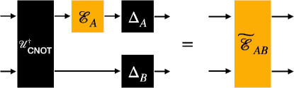
Figure 5: Measurement-coherence generating power of a quantum channel $\mathcal{E}_{A}$ is converted to the measurement-entanglement generating power of a bipartite channel $\widetilde{\mathcal{E}}_{AB}$.

Theorem 7.

For a quantum channel $\mathcal{E}_{A}$, it holds that

$$C(\mathcal{E}_{A})=\max_{\mathcal{\mathcal{K_{AB},\mathcal{L}_{AB}}}}E(\Delta_{AB}\circ\mathcal{K}_{AB}\circ\mathcal{E}_{A}\circ\mathcal{L}_{AB}),$$ (121)

where the maximum is taken over a detection-incoherent operation $\mathcal{K}_{AB}$ and a unital detection-incoherent operation $\mathcal{L}_{AB}$. The maximum is achieved as follows:

$$C(\mathcal{E}_{A})=E(\Delta_{AB}\circ\mathcal{E}_{A}\circ\mathcal{U}^{{\dagger}}_{\mathrm{CNOT}}).$$ (122)

Note that $\mathcal{U}_{\mathrm{CNOT}}^{{\dagger}}$ is in $\mathbf{DIO}$ since $\mathcal{U}_{\mathrm{CNOT}}$ is in $\mathbf{MIO}$. This result says that the measurement-coherence generating power of a quantum channel $\mathcal{E}_{A}$ can be converted into the measurement-entanglement generating power of a bipartite channel without any additional measurement-coherence generating powers. The post-dephasing channels on the right-hand side act on a quantum measurement, making it incoherent with respect to the incoherent basis. This allows the adjoint channel of the generalized CNOT channel $\mathcal{U}_{\mathrm{CNOT}}^{{\dagger}}$ to effectively entangle each POVM element.

Next, we show that a measurement-entanglement generating power induces a measurement-coherence generating power.

Theorem 8.

A measurement-entanglement generating power monotone $\widetilde{E}$ induces a measurement-coherence generating power monotone $\widetilde{C}$ given by

$$\widetilde{C}(\mathcal{E}_{A})=\max_{\mathcal{\mathcal{K_{AB},\mathcal{L}_{AB}}}}\widetilde{E}(\Delta_{AB}\circ\mathcal{K}_{AB}\circ\mathcal{E}_{A}\circ\mathcal{L}_{AB}),$$ (123)

where the maximum is taken over a detection-incoherent operation $\mathcal{K}_{AB}$ and a unital detection-incoherent operation $\mathcal{L}_{AB}$.

The proof of Theorem 8 needs the following fact:

Proposition 9.

For a bipartite quantum channel $\mathcal{E}_{AB}$, $\Delta_{AB}\circ\mathcal{E}_{AB}\circ\Delta_{AB}\in\mathbf{SepC}(A\!:\!B)$.

Proof.

A quantum channel $\mathcal{N}_{A}$ is a classical channel if it satisfies the equation $\mathcal{N}_{A}=\Delta_{A}\circ\mathcal{N}_{A}\circ\Delta_{A}$ [71]. Since $\Delta_{AB}\circ\mathcal{E}_{AB}\circ\Delta_{AB}$ is a classical channel, its Choi-Jamiołkowski state is incoherent because

$$J^{AA^{\prime}BB^{\prime}}_{\mathcal{E}_{AB}} =\Delta_{AB}\circ\mathcal{E}_{AB}\circ\Delta_{AB}(\Phi^{d}_{AA^{\prime}}\otimes\Phi^{d}_{BB^{\prime}})$$ (124)

$$=\Delta_{AB}\otimes\Delta_{A^{\prime}B^{\prime}}\circ\mathcal{E}_{AB}(\Phi^{d}_{AA^{\prime}}\otimes\Phi^{d}_{BB^{\prime}}).$$ (125)

Thus, $J_{AA^{\prime}BB^{\prime}}^{\mathcal{E}_{AB}}$ is separable. A separable Choi-Jamiołkowski state corresponds to a separable channel. ∎

Here’s the proof of Theorem 8:

Proof.

1. Non-negativity and faithfulness can be shown as follows: $\widetilde{C}(\mathcal{E}_{A})\geq 0$ due to the non-negativity of the entanglement monotone $\widetilde{E}$. If $\mathcal{E}_{A}\in\mathbf{DIO}$, then

   $$\Delta_{AB}\circ\mathcal{K}_{AB}\circ\mathcal{E}_{A}\circ\mathcal{L}_{AB}=\Delta_{AB}\circ\mathcal{K}_{AB}\circ\mathcal{E}_{A}\circ\mathcal{L}_{AB}\circ\Delta_{AB}$$ (126)

   is a separable channel by Proposition 9. Therefore $\widetilde{C}(\mathcal{E_{A}})=0$. If $\mathcal{E}_{A}\notin\mathbf{DIO}$, then Theorem 7 implies that $\Delta_{AB}\circ\mathcal{E}_{A}\circ\mathcal{U}_{\mathrm{CNOT}}\notin\mathbf{SepC}(A\!:\!B)$, thereby $\widetilde{C}(\mathcal{E}_{A})>0$.

2. Convexity holds due to convexity of the entanglement monotone $\widetilde{E}$.

3. For a detection-incoherent channel $\mathcal{K}^{\prime}_{A}$ and a unital detector-incoherent channel $\mathcal{L}^{\prime}_{A}$, the monotonicity holds as

   $$\widetilde{C}(\mathcal{K}^{\prime}_{A}\circ\mathcal{E}_{A}\circ\mathcal{L}^{\prime}_{A}) =\max_{\mathcal{\mathcal{K_{AB},\mathcal{L}_{AB}}}}E(\Delta_{AB}\circ\mathcal{K}_{AB}\circ(\mathcal{K}^{\prime}_{A}\circ\mathcal{E}_{A}\circ\mathcal{L}^{\prime}_{A})\circ\mathcal{L}_{AB})$$ (127)

   $$\leq\widetilde{C}(\mathcal{E}_{A}),$$ (128)

   because $\mathcal{K}^{\prime}_{A}$ and $\mathcal{L}^{\prime}_{A}$ reduce the domain of maximization of $\mathcal{K}_{AB}$ and $\mathcal{L}_{AB}$, respectively.

∎

Reduction of measurement-resource generating power to measurement-resource

When we consider a measurement channel $\mathcal{N}_{A}$ with output system $A^{\prime}$, Theorem 7 reduces to the measurement-coherence conversion to measurement-entanglement [56]. It holds because $\mathcal{N}_{A}=\Delta_{A^{\prime}}\circ\mathcal{N}_{A}=\mathcal{I}_{A^{\prime}}\circ\mathcal{N}_{A}$.

The measurement-coherence generating power of a measurement channel $\mathcal{N}_{A}$ reduces to the measurement-coherence of the measurement channel $\mathcal{N}_{A}$ by Lemma 3 as follows:

$$C(\mathcal{N}_{A}) =C_{m}(\mathcal{I}_{A^{\prime}}\circ\mathcal{N}_{A})$$ (129)

$$=C_{m}(\mathcal{N}_{A}).$$ (130)

Similarly, the measurement-entanglement generating power $E(\mathcal{N}_{AB})$ of a measurement channel $\mathcal{N}_{AB}$ reduces to the measurement-entanglement $E_{m}(\mathcal{N}_{AB})$ of a measurement channel $\mathcal{N}_{AB}$. We first prove that $E(\mathcal{N}_{AB})\leq E_{m}(\mathcal{N}_{AB})$:

$$E(\mathcal{N}_{AB}) \coloneqq\min_{\mathcal{F}\in\mathbf{SepC}(A:B)}\max_{\mathcal{M}\in\mathbf{SepM}(A\widetilde{A}:B\widetilde{B})}$$ (131)

$$\qquad D_{m}(\mathcal{M}_{A\widetilde{A}B\widetilde{A}}\circ\mathcal{N}_{AB}\|\mathcal{M}_{A\widetilde{A}B\widetilde{B}}\circ\mathcal{F}_{AB})$$ (132)

$$\leq\min_{\mathcal{F}\in\mathbf{SepM}(A:B)}\max_{\mathcal{M}\in\mathbf{SepM}(A\widetilde{A}:B\widetilde{B})}$$ (133)

$$\qquad D_{m}(\mathcal{M}_{A\widetilde{A}B\widetilde{A}}\circ\mathcal{N}_{AB}\|\mathcal{M}_{A\widetilde{A}B\widetilde{B}}\circ\mathcal{F}_{AB})$$ (134)

$$=\min_{\mathcal{F}\in\mathbf{SepM}(A:B)}\max_{\mathcal{M}\in\mathbf{SepM}(A\widetilde{A}:B\widetilde{B})}$$ (135)

$$\qquad D_{m}(\mathcal{M}_{A\widetilde{A}B\widetilde{B}}\circ\Delta_{AB}\circ\mathcal{N}_{AB}\|\mathcal{M}_{A\widetilde{A}B\widetilde{B}}\circ\Delta_{AB}\circ\mathcal{F}_{AB})$$ (136)

$$=\min_{\mathcal{F}\in\mathbf{SepM}(A:B)}\max_{\mathcal{M}\in\mathbf{SepM}(A:B)}$$ (137)

$$\qquad D_{m}(\mathcal{M}_{AB}\circ\Delta_{AB}\circ\mathcal{N}_{AB}\|\mathcal{M}_{AB}\circ\Delta_{AB}\circ\mathcal{F}_{AB})$$ (138)

$$=\min_{\mathcal{F}\in\mathbf{SepM}(A\!:\!B)}\max_{\mathcal{S}_{A},\mathcal{S}_{B}\in\mathbf{S}}$$ (139)

$$\qquad D_{m}(\mathcal{S}_{A}\otimes\mathcal{S}_{B}\circ\Delta_{AB}\circ\mathcal{N}_{AB}\|\mathcal{S}_{A}\otimes\mathcal{S}_{B}\circ\Delta_{AB}\circ\mathcal{F}_{AB})$$ (140)

$$=\min_{\mathcal{F}\in\mathbf{SepM}(A\!:\!B)}D_{m}(\mathcal{N}_{AB}\|\mathcal{F}_{AB})$$ (141)

$$=E_{m}(\mathcal{N}_{AB}),$$ (142)

where the third equality follows from Lemma 5 and the fact that measurement channels output incoherent states. The fourth equality holds from Corollary 2. The fifth equality follows from the monotonicity of $D_{m}$ under classical post-processing channel.

The opposite direction is proved as follows:

$$E(\mathcal{N}_{AB}) \coloneqq\min_{\mathcal{F}\in\mathbf{SepC}(A:B)}\max_{\mathcal{M}\in\mathbf{SepM}(A\widetilde{A}:B\widetilde{B})}$$ (143)

$$\qquad D_{m}(\mathcal{M}_{A\widetilde{A}B\widetilde{A}}\circ\mathcal{N}_{AB}\|\mathcal{M}_{A\widetilde{A}B\widetilde{B}}\circ\mathcal{F}_{AB})$$ (144)

$$\geq\min_{\mathcal{F}\in\mathbf{SepC}(A:B)}\max_{\mathcal{M}\in\mathbf{SepM}(A\widetilde{A}:B\widetilde{B})}$$ (145)

$$\qquad D_{m}(\mathcal{M}_{A\widetilde{A}B\widetilde{B}}\circ\Delta_{AB}\circ\mathcal{N}_{AB}\|\mathcal{M}_{A\widetilde{A}B\widetilde{B}}\circ\Delta_{AB}\circ\mathcal{F}_{AB})$$ (146)

$$=\min_{\mathcal{F}\in\mathbf{SepC}(A:B)}\max_{\mathcal{M}\in\mathbf{SepM}(A:B)}$$ (147)

$$\qquad D_{m}(\mathcal{M}_{AB}\circ\Delta_{AB}\circ\mathcal{N}_{AB}\|\mathcal{M}_{AB}\circ\Delta_{AB}\circ\mathcal{F}_{AB})$$ (148)

$$=\min_{\mathcal{F}\in\mathbf{SepM}(A:B)}\max_{\mathcal{M}\in\mathbf{SepM}(A:B)}$$ (149)

$$\qquad D_{m}(\mathcal{M}_{AB}\circ\Delta_{AB}\circ\mathcal{N}_{AB}\|\mathcal{M}_{AB}\circ\Delta_{AB}\circ\mathcal{F}_{AB})$$ (150)

$$=E_{m}(\mathcal{N}_{AB}),$$ (151)

where the first inequality holds due to $\mathcal{M}_{A\widetilde{A}B\widetilde{B}}\circ\Delta_{AB}\in\mathbf{SepM}(A\widetilde{A}:B\widetilde{B})$, the second equality follows from Lemma 5. The third equality holds because of $\Delta_{AB}\circ\mathcal{F}_{AB}\in\mathbf{SepM}(A\!:\!B)$.

Relation between coherence generating power and measurement-coherence generating power

Here we investigate the relation between a quantum channel’s state-resource and measurement-resource generating powers. We begin by defining the coherence generating power of a quantum channel $\mathcal{E}_{A}$ as

$$C_{g}(\mathcal{E}_{A})\coloneqq\max_{\sigma_{A\widetilde{A}}\in\textbf{I}}C_{R}(\mathcal{E}_{A}(\sigma_{A\widetilde{A}})),$$ (152)

where $C_{R}(\rho_{A})\coloneqq\min_{\sigma_{A}\in\mathbf{I}}D(\rho_{A}|\sigma_{A})$ is the relative entropy of coherence [12], and $\mathbf{I}$ is the set of incoherent states. The coherence generating power of a quantum channel $\mathcal{E}_{A}$ can be written as

$$C_{g}(\mathcal{E}_{A})=\max_{\left|i\right\rangle\!\left\langle i\right|_{A}\in\textbf{I}}C_{R}(\mathcal{E}_{A}(\left|i\right\rangle\!\left\langle i\right|_{A})).$$ (153)

This can be shown as follows:

$$C_{g}(\mathcal{E}_{A}) \coloneqq\max_{\sigma_{A\widetilde{A}}\in\textbf{I}}C_{R}(\mathcal{E}_{A}(\sigma_{A\widetilde{A}}))$$ (154)

$$=C_{R}(\mathcal{E}_{A}(\sigma_{A\widetilde{A}}^{\ast}))$$ (155)

$$=C_{R}\left(\mathcal{E}_{A}\left(\sum_{i,j}p_{ij}\left|ij\right\rangle\!\left\langle ij\right|_{A\widetilde{A}}\right)\right)$$ (156)

$$\leq\sum_{i,j}p_{ij}C_{R}(\mathcal{E}_{A}(\left|ij\right\rangle\!\left\langle ij\right|_{A\widetilde{A}}))$$ (157)

$$\leq\max_{\left|i\right\rangle\!\left\langle i\right|_{A}\in\textbf{I}}C_{R}(\mathcal{E}_{A}(\left|i\right\rangle\!\left\langle i\right|_{A})),$$ (158)

where $\sigma_{A\widetilde{A}}^{\ast}$ is an optimal argument in the definition of $C_{g}(\mathcal{E}_{A})$. The other direction $C_{g}(\mathcal{E}_{A})\geq\max_{\left|i\right\rangle\!\left\langle i\right|_{A}\in\textbf{I}}C_{R}(\mathcal{E}_{A}(\left|i\right\rangle\!\left\langle i\right|_{A}))$ holds because the domain of the maximization in the definition of $C_{g}$ includes the incoherent basis.

In general, there is no relation between a quantum channel’s coherence generating power and measurement-coherence generating power. This can be seen by examining some quantum channels. Consider the following preparation channel:

$$\mathcal{E}_{A}(\rho_{A})=\langle 0\rvert\rho_{A}\lvert 0\rangle_{A}\left|+\right\rangle\!\left\langle+\right|_{A}+\langle 1\rvert\rho_{A}\lvert 1\rangle_{A}\left|+\right\rangle\!\left\langle+\right|_{A}=\left|+\right\rangle\!\left\langle+\right|_{A}.$$ (159)

The quantum channel $\mathcal{E}_{A}$ has maximum coherence generating power as

$$C_{g}(\mathcal{E}_{A})=\max_{\sigma_{A}\in\text{I}}C_{R}(\mathcal{E}_{A}(\rho)_{A})=1,$$ (160)

while its measurement-coherence generating power is zero as

$$C(\mathcal{E}_{A})=C_{m}(\mathcal{I}_{A}\circ\mathcal{E}_{A})=0,$$ (161)

because $\mathcal{I}_{A}\circ\mathcal{E}_{A}=\{\frac{I_{A}}{2},\frac{I_{A}}{2}\}$.

Similarly, one can conceive a quantum channel $\mathcal{G}_{A}$ such that

$$\mathcal{G}_{A}(\rho_{A})=\langle+\rvert\rho_{A}\lvert+\rangle_{A}\left|0\right\rangle\!\left\langle 0\right|_{A}+\langle-\rvert\rho_{A}\lvert-\rangle_{A}\left|1\right\rangle\!\left\langle 1\right|_{A}.$$ (162)

The quantum channel $\mathcal{G}_{A}$ does not generate any quantum coherence while it can generate measurement-coherence as

$$\mathcal{I}_{A}\circ\mathcal{G}_{A}=\{\left|+\right\rangle\!\left\langle+\right|_{A},\left|-\right\rangle\!\left\langle-\right|_{A}\}.$$ (163)

Thus, it is not possible to assert a relation between the coherence generating power and measurement-coherence generating power of a quantum channel. However, it can be observed that a unital quantum channel is related to its adjoint channel in terms of static resource generating powers as follows:

Theorem 10.

For a unital quantum channel $\mathcal{E}_{A}$, the coherence generating power of $\mathcal{E}_{AB}$ and measurement-coherence generating power of its adjoint channel $\mathcal{E}_{A}^{{\dagger}}$ satisfy the following relation:

$$\dfrac{1}{d}C_{g}(\mathcal{E}_{A})\leq C(\mathcal{E}_{A}^{{\dagger}})\leq C_{g}(\mathcal{E}_{A}).$$ (164)

Proof.

It holds that

$$C(\mathcal{E}_{A}^{{\dagger}}) =C_{m}(\mathcal{I}_{A}\circ\mathcal{E}_{A}^{{\dagger}})$$ (165)

$$=\dfrac{1}{d}\sum_{i=0}^{d-1}C_{R}(\mathcal{E}_{A}(\left|i\right\rangle\!\left\langle i\right|_{A}))$$ (166)

$$\leq C_{g}(\mathcal{E}_{A}),$$ (167)

where the inequality follows from Eq. (153). The lower bound follows from Eq. (153) and the non-negativity of $C_{R}$. ∎

This shows that a unital quantum channel having no coherence generating power can not generate measurement-coherence neither, vice versa.

Entanglement generating power of a quantum channel $\mathcal{E}_{AB}$ can be defined as

$$E_{g}(\mathcal{E}_{AB})=\max_{\sigma\in\mathbf{SepD}(A\widetilde{A}:B\widetilde{B})}E_{R}(\mathcal{E}_{AB}(\sigma_{A\widetilde{A}B\widetilde{B}})).$$ (168)

The ancillary system in the definition is necessary to capture the entanglement generating power of a quantum channel in a situation where the quantum channel acts on subsystems of a large system. Typical example is the SWAP gate on system $AB$. It does not generate entanglement from $\sigma_{AB}\in\mathbf{SepD}(A\!:\!B)$ while it can generate the maximum entanglement from $\sigma_{A\widetilde{A}B\widetilde{B}}\in\mathbf{SepD}(A\widetilde{A}\!:\!B\widetilde{B})$ [72].

A quantum channel’s entanglement generating power bounds its adjoint channel’s measurement-entanglement generating power as follows:

Theorem 11.

For a unital quantum channel $\mathcal{E}_{AB}$, entanglement generating power is equal or larger than measurement-entanglement generating power of its adjoint channel $\mathcal{E}_{AB}^{{\dagger}}$:

$$E(\mathcal{E}_{AB}^{{\dagger}})\leq E_{g}(\mathcal{E}_{AB}).$$ (169)

Proof.

Let $\mathbf{USepC}(A:B)=\{\mathcal{F}_{AB}\in\mathbf{SepC}(A:B):\mathcal{F}_{AB}(I_{AB})=I_{AB}\}$ be the set of unital separable channels. The following holds that:

$$E(\mathcal{E}_{AB}^{{\dagger}}) =\min_{\mathcal{F}\in\mathbf{SepC}(A:B)}\max_{\mathcal{M}\in\mathbf{SepM}(A\widetilde{A}:B\widetilde{B})}$$ (170)

$$\qquad D_{m}(M_{A\widetilde{A}B\widetilde{B}}\circ\mathcal{E}_{AB}^{{\dagger}}\|\mathcal{M}_{A\widetilde{A}B\widetilde{B}}\circ\mathcal{F}_{AB})$$ (171)

$$\leq\min_{\mathcal{F}\in\mathbf{USepC}(A:B)}\max_{\mathcal{M}\in\mathbf{SepM}(A\widetilde{A}:B\widetilde{B})}$$ (172)

$$\qquad D_{m}(M_{A\widetilde{A}B\widetilde{B}}\circ\mathcal{E}_{AB}^{{\dagger}}\|\mathcal{M}_{A\widetilde{A}B\widetilde{B}}\circ\mathcal{F}_{AB})$$ (173)

$$=D_{m}(\mathcal{E}_{AB}(\mathcal{M}_{A\widetilde{A}B\widetilde{B}}^{\ast})\|\mathcal{F}_{AB}^{\ast{\dagger}}(\mathcal{M}_{A\widetilde{A}B\widetilde{B}}^{\ast}))$$ (174)

$$=\dfrac{1}{d^{4}}\sum_{x,y}D(\mathcal{E}_{AB}(M_{xy}^{\ast})\|\mathcal{F}_{AB}^{\ast{\dagger}}(M_{xy}^{\ast}))$$ (175)

$$\leq\max_{x,y}D\left(\mathcal{E}_{AB}\left(\dfrac{M_{xy}^{\ast}}{d^{4}}\right)\bigg{\|}\mathcal{F}_{AB}^{\ast{\dagger}}\left(\dfrac{M_{xy}^{\ast}}{d^{4}}\right)\right)$$ (176)

$$=D(\mathcal{E}_{AB}(M_{0}^{\ast})\|\mathcal{F}_{AB}^{\ast{\dagger}}(M_{0}^{\ast})).$$ (177)

Let $M_{0}^{\ast}=q_{0}\sigma_{A\widetilde{A}B\widetilde{B}}$, where $q_{0}=\operatorname{Tr}M_{0}^{\ast}\leq 1$ and $\sigma_{A\widetilde{A}B\widetilde{B}}=M_{0}^{\ast}/q_{0}$ is a separable state in $\mathbf{SepD}(A\widetilde{A}\!:\!B\widetilde{B})$. Then it follows that

$$E(\mathcal{E}_{AB}^{{\dagger}}) \leq D(\mathcal{E}_{AB}(q_{0}\sigma_{A\widetilde{A}B\widetilde{B}})\|\mathcal{F}_{AB}^{\ast{\dagger}}(q_{0}\sigma_{A\widetilde{A}B\widetilde{B}}))$$ (178)

$$=q_{0}D(\mathcal{E}_{AB}(\sigma_{A\widetilde{A}B\widetilde{B}})\|\mathcal{F}_{AB}^{\ast{\dagger}}(\sigma_{A\widetilde{A}B\widetilde{B}}))$$ (179)

$$\leq E_{g}(\mathcal{E}_{AB}).$$ (180)

∎

References

[1]
Johann von Neumann and Robert T. Beyer.
Mathematische Grundlagen Der Quantenmechanik.
Mathematical Foundations of Quantum Mechanics … Translated …
by Robert T. Beyer.
1955.
[2]
Norman F. Ramsey.
A Molecular Beam Resonance Method with Separated Oscillating
Fields.
Physical Review, 78(6):695–699, June 1950.
[3]
Chao Zhang, Thomas R. Bromley, Yun-Feng Huang, Huan Cao, Wei-Min Lv, Bi-Heng
Liu, Chuan-Feng Li, Guang-Can Guo, Marco Cianciaruso, and Gerardo Adesso.
Demonstrating Quantum Coherence and Metrology that is
Resilient to Transversal Noise.
Physical Review Letters, 123(18):180504, November 2019.
[4]
Mark Hillery.
Coherence as a resource in decision problems: The Deutsch-Jozsa
algorithm and a variation.
Physical Review A, 93(1):012111, January 2016.
[5]
Hai-Long Shi, Si-Yuan Liu, Xiao-Hui Wang, Wen-Li Yang, Zhan-Ying Yang, and Heng
Fan.
Coherence depletion in the Grover quantum search algorithm.
Physical Review A, 95(3):032307, March 2017.
[6]
Felix Ahnefeld, Thomas Theurer, Dario Egloff, Juan Mauricio Matera, and
Martin B. Plenio.
Coherence as a Resource for Shor’s Algorithm.
Physical Review Letters, 129(12):120501, September 2022.
[7]
C. K. Hong, Z. Y. Ou, and L. Mandel.
Measurement of subpicosecond time intervals between two photons by
interference.
Physical Review Letters, 59(18):2044–2046, November 1987.
[8]
Gilad Gour.
Role of Quantum Coherence in Thermodynamics.
PRX Quantum, 3(4):040323, November 2022.
[9]
Gilad Gour.
Erratum: Role of Quantum Coherence in Thermodynamics
[PRX Quantum 3, 040323 (2022)].
PRX Quantum, 4(4):040901, October 2023.
[10]
Federico Levi and Florian Mintert.
A quantitative theory of coherent delocalization.
New Journal of Physics, 16(3):033007, 2014.
[11]
Johan Aberg.
Quantifying Superposition.
arXiv:quant-ph/0612146, December 2006.
arXiv: quant-ph/0612146.
[12]
T. Baumgratz, M. Cramer, and M. B. Plenio.
Quantifying Coherence.
Physical Review Letters, 113(14):140401, September 2014.
[13]
Andreas Winter and Dong Yang.
Operational Resource Theory of Coherence.
Physical Review Letters, 116(12):120404, March 2016.
[14]
Eric Chitambar and Gilad Gour.
Comparison of incoherent operations and measures of coherence.
Physical Review A, 94(5):052336, November 2016.
[15]
T. Theurer, N. Killoran, D. Egloff, and M. B. Plenio.
Resource Theory of Superposition.
Physical Review Letters, 119(23):230401, December 2017.
[16]
Felix Bischof, Hermann Kampermann, and Dagmar Bruß.
Resource Theory of Coherence Based on
Positive-Operator-Valued Measures.
Physical Review Letters, 123(11):110402, September 2019.
[17]
Kok Chuan Tan, Tyler Volkoff, Hyukjoon Kwon, and Hyunseok Jeong.
Quantifying the Coherence between Coherent States.
Physical Review Letters, 119(19):190405, November 2017.
[18]
Huangjun Zhu, Zhihao Ma, Zhu Cao, Shao-Ming Fei, and Vlatko Vedral.
Operational one-to-one mapping between coherence and entanglement
measures.
Physical Review A, 96(3):032316, September 2017.
[19]
Huangjun Zhu, Masahito Hayashi, and Lin Chen.
Coherence and entanglement measures based on Rényi relative
entropies.
Journal of Physics A: Mathematical and Theoretical,
50(47):475303, 2017.
[20]
Alexander Streltsov, Gerardo Adesso, and Martin B. Plenio.
Colloquium: Quantum coherence as a resource.
Reviews of Modern Physics, 89(4):041003, October 2017.
[21]
Charles H. Bennett, Gilles Brassard, Claude Crépeau, Richard Jozsa, Asher
Peres, and William K. Wootters.
Teleporting an unknown quantum state via dual classical and
einstein-podolsky-rosen channels.
Physical Review Letters, 70(13):1895, 1993.
[22]
Artur K. Ekert and Peter L. Knight.
Relationship between semiclassical and quantum-mechanical
input-output theories of optical response.
Physical Review A, 43(7):3934–3938, April 1991.
[23]
Benjamin K. Malia, Yunfan Wu, Julián Martínez-Rincón, and Mark A.
Kasevich.
Distributed quantum sensing with mode-entangled spin-squeezed atomic
states.
Nature, 612(7941):661–665, December 2022.
[24]
Robert Raussendorf and Hans J. Briegel.
A one-way quantum computer.
Physical Review Letters, 86(22):5188–5191, May 2001.
[25]
H. J. Briegel, D. E. Browne, W. Dur, R. Raussendorf, and M. Van den Nest.
Measurement-based quantum computation.
Nat Phys, pages 19–26, online January 02, 2009.
[26]
Hsin-Yuan Huang.
Information-Theoretic Bounds on Quantum Advantage in
Machine Learning.
Physical Review Letters, 126(19), 2021.
[27]
Hsin-Yuan Huang, Michael Broughton, Jordan Cotler, Sitan Chen, Jerry Li, Masoud
Mohseni, Hartmut Neven, Ryan Babbush, Richard Kueng, John Preskill, and
Jarrod R. McClean.
Quantum advantage in learning from experiments.
Science (New York, N.Y.), 376(6598):1182–1186, June 2022.
[28]
Dorit Aharonov, Jordan Cotler, and Xiao-Liang Qi.
Quantum algorithmic measurement.
Nature Communications, 13(1):887, February 2022.
[29]
Sitan Chen, Jordan Cotler, Hsin-Yuan Huang, and Jerry Li.
Exponential Separations Between Learning With and Without
Quantum Memory.
In 2021 IEEE 62nd Annual Symposium on Foundations of
Computer Science (FOCS), pages 574–585, February 2022.
[30]
G. Vidal, J. I. Latorre, E. Rico, and A. Kitaev.
Entanglement in Quantum Critical Phenomena.
Physical Review Letters, 90(22):227902, June 2003.
[31]
J. Ignacio Cirac, David Pérez-García, Norbert Schuch, and Frank
Verstraete.
Matrix product states and projected entangled pair states:
Concepts, symmetries, theorems.
Reviews of Modern Physics, 93(4):045003, December 2021.
[32]
A.Yu. Kitaev.
Fault-tolerant quantum computation by anyons.
Annals of Physics, 303(1):2–30, January 2003.
[33]
Guifré Vidal.
Efficient Classical Simulation of Slightly Entangled Quantum
Computations.
Physical Review Letters, 91(14):147902, October 2003.
[34]
Guifré Vidal.
Efficient Simulation of One-Dimensional Quantum Many-Body
Systems.
Physical Review Letters, 93(4):040502, July 2004.
[35]
M. S. Kim, W. Son, V. Bužek, and P. L. Knight.
Entanglement by a beam splitter: Nonclassicality as a
prerequisite for entanglement.
Physical Review A, 65(3):032323, February 2002.
[36]
János K. Asbóth, John Calsamiglia, and Helmut Ritsch.
Computable Measure of Nonclassicality for Light.
Physical Review Letters, 94(17):173602, May 2005.
[37]
W. Vogel and J. Sperling.
Unified quantification of nonclassicality and entanglement.
Physical Review A, 89(5):052302, May 2014.
[38]
N. Killoran, F. E. S. Steinhoff, and M. B. Plenio.
Converting Nonclassicality into Entanglement.
Physical Review Letters, 116(8):080402, February 2016.
[39]
V. Vedral, M. B. Plenio, M. A. Rippin, and P. L. Knight.
Quantifying entanglement.
Physical Review Letters, 78(12):2275–2279, 1997.
[40]
Ryszard Horodecki, Paweł Horodecki, Michał Horodecki, and Karol
Horodecki.