Implicit-explicit time discretization schemes for a class of semilinear wave equations with nonautonomous dampings

Abstract

This paper is concerned about the implicit-explicit (IMEX) methods for a class of dissipative wave systems with time-varying velocity feedbacks and nonlinear potential energies, equipped with different boundary conditions. Firstly, we approximate the problems by using a vanilla IMEX method, which is a second-order scheme for the problems when the damping terms are time-independent. However, rigors analysis shows that the error rate declines from second to first order due to the nonautonomous dampings. To recover the convergence order, we propose a revised IMEX scheme and apply it to the nonautonomous wave equations with a kinetic boundary condition. Our numerical experiments demonstrate that the revised scheme can not only achieve second-order accuracy but also improve the computational efficiency.

Introduction

In this paper we consider numerical solutions for the following semilinear evolution equation of second-order

$$\ddot{u}(t)+B(t)\dot{u}(t)+Au(t)=f(t,u(t))$$

in a suitable Hilbert space. Such evolution equation is renowned for their prevalence in a spectrum of mathematical models derived from physics, elastodynamics, acoustics etc, for example, the propagation of dislocations in crystals [1], wave motions in a dissipative medium [2], and structural acoustic interactions [3], thereby providing a versatile abstract framework that encompasses a multitude of wave-type equations wave-type equations with a diverse array of boundary conditions such as Dirichlet, Neumann, Robin and dynamic boundary conditions.

The theoretical exploration of the semilinear evolution equation has attracted many researchers’ attention over an extended period. (cf. [4, 5, 6, 7, 8, 9, 10]), while the numerical analysis on this evolution equation can be broadly classified into two main categories based on the boundary conditions. In the first category, it is concerned with wave-type equations subject to Dirichlet, Neumann or Robin boundary conditions. There are numerous investigations on numerical methods for these equations including finite difference methods [11, 12], finite element methods [13, 14], characteristic methods [15, 16], spectral methods [17, 18] and the methods of lines [19, 20], among others. The second category focuses on wave equations with dynamic boundary conditions. A series of papers [21, 22, 23, 24] have been published recently to provide a comprehensive error analysis on some discrete schemes for this type of wave equations. It is noteworthy that the damping terms are time-independent in all these papers. In light of this, this paper is aimed to investigate the numerical schemes for semilinear wave-type equations with time-varying dampings and subject to dynamic boundary conditions, addressing a gap in the current literature.

It is a well-established fact that explicit schemes usually suffer severe time step restrictions despite their computational simplicity, and full implicit schemes are always unconditionally stable but rather taxing and time consuming. Against this backdrop, the focus of this paper is on an IMEX time discretization scheme. This approach is a popular and widely-used approach (cf. [25, 26, 27, 28]), which leverages an implicit treatment for the unbounded linear components and an explicit treatment for the nonlinear aspects of a differential equation. For‌ an in-depth investigation of the IMEX scheme, we direct the readers to seminal works: [29] for IMEX Runge-Kutta schemes, [30] for IMEX multistep schemes, [31] for Crank-Nicolson-leapfrog IMEX scheme, and references therein.

Closely pertinent to our investigation, we refer to a recent study [32], where an IMEX scheme is introduced. This scheme is crafted by merging the Crank-Nicolson method for linear segments and the leapfrog method for nonlinear components, culminating in a second-order numerical scheme. However, when this IMEX scheme is applied to a class of semilinear wave equations with nonautonomous damping terms, it is noted that the error rate descends to the first order, as will be elaborated in Section 4. Thus, it is both natural and necessary to delve into the influence that nonautonomous damping terms exert on the convergence rate of the IMEX scheme.

Motivated by previous research, this paper aims to present a comprehensive discretization of the aforementioned semilinear evolution equation in an abstract manner. The key contributions of this study are encapsulated as follows: The major contributions of this article can be summarized as follows: (i) Our methodology offers a cohesive approach to solve a class of wave-type equations with time-dependent dampings and subject to different types of boundary conditions. (ii) We conduct an error analysis on the full discretization with a vanilla IMEX scheme, which reveals the time-varying damping coefficients play a fundamental role in making the error oder decrease to be one. (iii) The full discretization with a revised IMEX scheme is a second-order method that is more computationally efficient without compromising the order of convergence. We collect the obtained error estimates for the temporal discretization in Table 1, and mark whether these results are discussed theoretically or illustrated numerically.

Scheme	autonomous damping	nonautonomous damping	Discussed in	illustrated
IMEX	$\tau^{2}$	$\tau$	Theorem 3.1	✓
Revised IMEX	$\tau^{2}$	$\tau^{2}$	✗	✓

Table 1: Overview of convergence rate for time discretization schemes with step size $\tau$.

This paper is structured as follows. In Section 2, we begin by introducing semilinear evolution equations as an abstract framework for wave-type equations with time-dependent damping, and then present three exemplary wave equations with distinct boundary conditions. Section 3 commences with an overview of a general space discretization. Subsequently, we develop two full discrete schemes by combing the vanilla and revised IMEX with the abstract space discretization. An error analysis of these full discretizations will be also given. Numerical examples are presented in Section 4 to substantiate the error bounds derived from our main theorem. These examples will not only highlight the error rate but also showcase the efficacy of the proposed schemes. The focus of Section 5 is on the detailed proof of our main result. For better readability, the Crank-Nicolson scheme and the vanilla IMEX scheme for the semilinear wave equations with nonautonomous dampings are detailed in A and B, respectively.

Preliminary

Let $V$, $H$ be Hilbert spaces with norms $\|\cdot\|_{V}$ and $\|\cdot\|_{H}$. The second norm induced by an inner product $m(\cdot,\cdot)$ on $H$, and $V$ is densely embedded in $H$. Moreover, we identify $H$ with its dual $H^{\ast}$ which gives the Gelfand triple

$$V\hookrightarrow H\equiv H^{\ast}\hookrightarrow V^{\ast}.$$

Here, the notation $\hookrightarrow$ means the dense embedding. Thus, there exists an embedding constant $C_{\mathrm{em}}>0$ such that $\|\upsilon\|_{H}\leqslant C_{\mathrm{em}}\|\upsilon\|_{V}$, and the duality $\langle\cdot,\cdot\rangle_{V}:V^{\ast}\times V\rightarrow\mathbb{R}$ coincide with $m(\cdot,\cdot)$ on $H\times V$.

The abstract wave equation that covers all examples in this paper can be written as follows.

$$\langle\ddot{u},\phi\rangle_{V}+b(\dot{u},\phi)+\gamma(t)m(\dot{u},\phi)+a(u,\phi) =\langle f(t,u),\phi\rangle_{V}\quad\textrm{for all $\phi\in V$, and $t\in(0,T]$,}$$ (1)

$$u(0)=u^{0},\quad\dot{u}(0) =v^{0}.$$

where the initial data $u^{0}\in V$, $v^{0}\in H$, $a:V\times V\rightarrow\mathbb{R}$ and $b:V\times V\rightarrow\mathbb{R}$ are continuous bilinear forms, and the nonlinearity $f:[0,T]\times V\rightarrow V^{\ast}$ is continuous. The notations $\dot{}=\frac{\mathrm{d}}{\mathrm{d}t}$ and $\ddot{}=\frac{\mathrm{d}^{2}}{\mathrm{d}t^{2}}$ denote the first and second temporal derivatives, respectively.

We define operators $A,B\in\mathcal{L}(V,V^{\ast})$ induced by the bilinear forms $a$ and $b$ via

$$\langle A\varphi,\phi\rangle_{V}=a(\varphi,\phi)\quad\textrm{and}\quad\langle B\varphi,\phi\rangle_{V}=b(\varphi,\phi)\quad\textrm{for all $\varphi,\phi\in V$}.$$

The variational equation (1) can be equivalently stated as an second-order evolution equation in $V^{\ast}$

$$\ddot{u}(t)+B(t)\dot{u}(t)+Au(t) =f(t,u(t)),\quad t\geqslant 0,$$ (2)

$$u(0)=u^{0},\quad\dot{u}(0) =v^{0}$$

with $B(t)=B+\gamma(t)I$. In addition, if we set $\dot{u}=v$ and define

$$\mathbf{u}=\left[\begin{array}[]{c}u\\ v\end{array}\right],\quad S=\left[\begin{array}[]{cc}0&-I\\ A&B\end{array}\right],\quad g(t,\mathbf{u})=\left[\begin{array}[]{c}0\\ f(t,u)-\gamma(t)v\end{array}\right],\quad\mathbf{u}^{0}=\left[\begin{array}[]{c}u^{0}\\ v^{0}\end{array}\right],$$

then (2) can be reformulated to be the following first-order equation in the Hilbert space $X=V\times H$.

$$\dot{\mathbf{u}}(t)+S\mathbf{u}(t) =g(t,\mathbf{u}(t)),\quad t\geqslant 0,$$ (3)

$$\mathbf{u}(0) =\mathbf{u}^{0}.$$

We need the following assumptions to guarantee the evolution equation (2) is locally wellposed.

• The bilinear form $a(\cdot,\cdot)$ is symmetric and there exists a constant $\alpha>0$ such that

  $$\mathrm{p}(\cdot,\cdot)=a(\cdot,\cdot)+\alpha m(\cdot,\cdot)$$

  is a inner product on $V$. Let the norm $\|\cdot\|_{V}$ be generated by this inner product.

• The bilinear form $b$ is bounded, that is,

  $$b(\upsilon,\omega)\leqslant C_{\mathrm{b}}\|\upsilon\|_{V}\|\omega\|_{H}\quad\textrm{for any $\upsilon\in V$, $\omega\in H$}$$

  and quasi-monotone which means there exists a constant $\beta>0$ for any $\upsilon\in V$

  $$b(\upsilon,\upsilon)+\beta m(\upsilon,\upsilon)\geqslant 0.$$

• The nonlinearity $f$ belongs to $C(V;H)$ and also is locally Lipschitz-continuous, that is, for any $\upsilon,\omega\in V$ satisfying $\|\upsilon\|_{V},\|\omega\|_{V}\leqslant\delta$ there exists a constant $C_{\delta}>0$ such that

  $$\|f(t,\upsilon)-f(t,\omega)\|_{H}\leqslant C_{\delta}\|\upsilon-\omega\|_{V}.$$

• The damping coefficient $\gamma(t)\in C^{2}_{loc}([0,\infty);\mathbb{R})$ satisfies

  $$\max_{t\in\mathcal{O}}\{\gamma(t),\dot{\gamma}(t),\ddot{\gamma}(t)\}\leqslant C_{\gamma},$$

  where $\mathcal{O}\subset[0,\infty)$ is any compact domain and $C_{\gamma}\geqslant 0$.

By the semigroup theory (e.g., [33, Section 6.1]) and regarding $f(t,u)-\gamma(t)v$ as a perturbation term, one can show the following lemma collecting a weak and a strong wellposedness result.

Lemma 2.1.

Let Assumptions $\mathrm{(H1)}$-$\mathrm{(H4)}$ be satisfied. Then for all $u^{0}\in V$, $v^{0}\in H$, (2) has a unique weak solution

$$u\in C^{2}\left([0,T];H^{\ast}\right)\cap C^{1}\left([0,T];H\right)\cap C\left([0,T];V\right)$$

with $T=T(u^{0},v^{0})$. Moreover, if $u^{0}\in D(A)$, $v^{0}\in V$, there exists a strong solution to (2)

$$u\in C^{2}\left([0,T];H\right)\cap C^{1}\left([0,T];V\right)\cap C\left([0,T];D(A)\right).$$

We present some examples of wave-type equation that can be written in the form of (1). First, we briefly introduce some notations. Let $\Omega$ be a bounded open region in $\mathbb{R}^{d}$, $d=2$ or $3$, with smooth boundary $\Gamma$. We denote by $\bigtriangledown_{\Gamma}$ the gradient on $\Gamma$, and the Laplace–Beltrami operator on $\Gamma$ is given by $\triangle_{\Gamma}=\bigtriangledown_{\Gamma}\cdot\bigtriangledown_{\Gamma}$. The outer normal is denoted by $\nu$.

• We consider the wave equation with a homogeneous Dirichlet boundary condition

$$u_{tt}+\gamma(t)u_{t}-c_{\Omega}\triangle u =f(t,u),\quad\textrm{in $\mathbb{R}^{+}\times\Omega$,}$$ (4)

$$u =0,\quad\textrm{on $\mathbb{R}^{+}\times\Gamma$,}$$

$$u(0,x)=u_{0}(x),\quad u_{t}(0,x) =u_{1}(x),\quad\textrm{in $\overline{\Omega}$.}$$

For the corresponding abstract formulation of (4), we choose $V=H^{1}_{0}(\Omega)$ and $H=L^{2}(\Omega)$. The product $m(\cdot,\cdot)$ is the standard $L^{2}(\Omega)$ inner product, the bilinear form $a(\cdot,\cdot)$ is given by $a(\upsilon,\omega)=c_{\Omega}\int_{\Omega}\bigtriangledown\upsilon\cdot\bigtriangledown\omega\mathrm{d}x$ and $b(\cdot,\cdot)$ equals to zero. Finally, the domain of $A$ is given by $D(A)=H^{1}_{0}(\Omega)\bigcap H^{2}(\Omega)$.

• The wave equation with kinetic boundary condition is considered

$$u_{tt}+\left[\alpha_{\Omega}+\beta_{\Omega}\cdot\bigtriangledown+\gamma(t)\right]u_{t}-c_{\Omega}\triangle u =f_{1}(t,u),\quad\textrm{in $\mathbb{R}^{+}\times\Omega$,}$$ (5)

$$\mu u_{tt}+(\alpha_{\Gamma}+\beta_{\Gamma}\cdot\bigtriangledown_{\Gamma})u_{t}-c_{\Gamma}\triangle_{\Gamma}u =-c_{\Omega}\partial_{\nu}u+f_{2}(t,u),\quad\textrm{on $\mathbb{R}^{+}\times\Gamma$,}$$

$$u(0,x)=u_{0}(x),\quad u_{t}(0,x) =u_{1}(x),\quad\textrm{in $\overline{\Omega}$.}$$

To write (5) as the abstract wave equation, we set $V=\{v\in H^{1}(\Omega):v|_{\Gamma}\in H^{1}(\Gamma)\}$ and $H=L^{2}(\Omega)\times L^{2}(\Gamma)$. The domain of $A$ is equal to the space $\{v\in H^{2}(\Omega):v|_{\Gamma}\in H^{2}(\Gamma)\}$. The inner product $m(\cdot,\cdot)$ is given by

$$m((v,\upsilon),(w,\omega))=\int_{\Omega}vw\mathrm{d}x+\mu\int_{\Gamma}\upsilon\omega\mathrm{d}\Gamma\quad\textrm{for any $(v,\upsilon),(w,\omega)\in H$}$$

and the bilinear forms

$$\begin{split}a(\upsilon,\omega)&=c_{\Omega}\int_{\Omega}\bigtriangledown\upsilon\cdot\bigtriangledown\omega\mathrm{d}x+c_{\Gamma}\int_{\Gamma}\bigtriangledown_{\Gamma}\upsilon\cdot\bigtriangledown_{\Gamma}\omega\mathrm{d}\Gamma\quad\textrm{for any $\upsilon\in V$, $\omega\in V$,}\\ b(\upsilon,\omega)&=\int_{\Omega}(\alpha_{\Omega}\upsilon+\beta_{\Omega}\cdot\bigtriangledown\upsilon)\omega\mathrm{d}x+\int_{\Gamma}(\alpha_{\Gamma}\upsilon+\beta_{\Gamma}\cdot\bigtriangledown_{\Gamma}\upsilon)\omega\mathrm{d}\Gamma\quad\textrm{for any $\upsilon\in V$, $\omega\in V$.}\end{split}$$

• Consider the wave equations with acoustic boundary conditions

$$u_{tt}+\gamma(t)u_{t}-c_{\Omega}\triangle u =f_{1}(t,u),\quad\textrm{in $\mathbb{R}^{+}\times\Omega$,}$$ (6)

$$\mu w_{tt}+dw_{t}+k_{\Gamma}w-c_{\Gamma}\triangle_{\Gamma}w =-c_{\Omega}u_{t}+f_{2}(t,u),\quad\textrm{on $\mathbb{R}^{+}\times\Gamma$,}$$

$$\partial_{\nu}u =w_{t},\quad\textrm{on $\mathbb{R}^{+}\times\Gamma$,}$$

$$u(0,x)=u_{0}(x),\quad u_{t}(0,x)=u_{1}(x),\quad w(0,x) =w_{0}(x),\quad w_{t}(0,x)=w_{1}(x),\quad\textrm{in $\overline{\Omega}$.}$$

We use the product spaces $V=H^{1}(\Omega)\times H^{1}(\Gamma)$, $H=L^{2}(\Omega)\times L^{2}(\Gamma)$ and $D(A)\subseteq H^{2}(\Omega)\times H^{2}(\Gamma)$. For any $\mathbf{v}=(v,\upsilon)\in H$, $\mathbf{w}=(w,\omega)\in H$, the inner product and and the bilinear forms are defined via

$$\begin{split}m(\mathbf{v},\mathbf{w})&=\int_{\Omega}vw\mathrm{d}x+\mu\int_{\Gamma}\upsilon\omega\mathrm{d}\Gamma,\\ a(\mathbf{v},\mathbf{w})&=c_{\Omega}\int_{\Omega}\bigtriangledown v\cdot\bigtriangledown w\mathrm{d}x+\int_{\Gamma}(k_{\Gamma}\upsilon\omega+c_{\Gamma}\bigtriangledown_{\Gamma}\upsilon\cdot\bigtriangledown_{\Gamma}\omega)\mathrm{d}\Gamma,\\ b(\mathbf{v},\mathbf{w})&=c_{\Omega}\int_{\Gamma}(v\omega-\upsilon w)\mathrm{d}\Gamma.\end{split}$$

Then we can write (6) as the abstract formulation.

Abstract full discretization

In this section, we integrate a vanilla or revised IMEX time scheme with an abstract space discretization to formulate a fully discrete scheme.

Abstract space discretization

Let $(V_{h})_{h}$ be a family of finite dimensional vector spaces for the spatial approximation with respect to a discretization parameter $h$. Then we consider the semidiscretized equation of (1)

$$\langle\ddot{u}_{h},\phi_{h}\rangle_{V_{h}}+b_{h}(\dot{u}_{h},\phi_{h})+\gamma(t)m_{h}(\dot{u}_{h},\phi_{h})+a_{h}(u_{h},\phi_{h}) =\langle f_{h}(t,u_{h}),\phi_{h}\rangle_{V_{h}}\quad t\in(0,T],$$ (7)

$$u_{h}(0)=u_{h}^{0},\quad\dot{u}_{h}(0) =v_{h}^{0}.$$

for all $\phi_{h}\in V_{h}$. Here, $a_{h}$, $b_{h}$ $f_{h}$, $m_{h}$, $\mathrm{p}_{h}$, $u_{h}^{0}$ and $v_{h}^{0}$ are the approximations of their corresponding continuous counterparts and share the similar properties as in Assumptions (H1)-(H3). The corresponding constants used in the discrete case are denoted by $\hat{\alpha}$, $\hat{\beta}$, $\hat{C}_{\mathrm{em}}$, $\hat{C}_{\mathrm{b}}$ and $\hat{C}_{\delta}$.

The semidiscretized equation (7) is equivalent to

$$\ddot{u}_{h}(t)+B_{h}\dot{u}_{h}(t)+\gamma(t)\dot{u}_{h}(t)+A_{h}u_{h}(t) =f_{h}(t,u_{h}(t)),\quad t\geqslant 0,$$ (8)

$$u_{h}(0)=u_{h}^{0},\quad\dot{u}_{h}(0) =v_{h}^{0}.$$

Analogously to the continuous case in Section 2, we set $\mathbf{u}_{h}=[u_{h},v_{h}]^{\top}$, $\mathbf{u}^{0}=[u^{0}_{h},v^{0}_{h}]^{\top}$ and

$$S_{h}=\left[\begin{array}[]{cc}0&-I\\ A_{h}&B_{h}\end{array}\right],\quad g_{h}(t,\mathbf{u}_{h})=\left[\begin{array}[]{c}0\\ f_{h}(t,u_{h})-\gamma(t)v_{h}\end{array}\right].$$

Let $H_{h}$ be the space $V_{h}$ equipped with the scalar product $m_{h}(\cdot,\cdot)$. Then we have the spatial discretization for the first-order evolution equation (3) in $X_{h}=V_{h}\times H_{h}$ as follows.

$$\dot{\mathbf{u}}_{h}+S_{h}\mathbf{u}_{h} =g_{h}(t,\mathbf{u}_{h}),\quad t\geqslant 0,$$ (9)

$$\mathbf{u}_{h}(0) =\mathbf{u}_{h}^{0}.$$

In the numerical experiments (see Section 4), we utilize the bulk-surface finite element method, as initially proposed in reference [34], to discretize semilinear wave equations within space $\Omega$. It is worth noting that the computational domain $\Omega_{h}$ is not identical to $\Omega$ but serves as an approximation. Consequently, the finite element functions in $X_{h}$ are defined in $\Omega_{h}$, not in $\Omega$. Then we have $X_{h}\nsubseteq X$, which complicates direct comparison between the approximation $\mathbf{u}_{h}\in X_{h}$ and the true solution $\mathbf{u}\in X$. To conduct an error analysis, some suitable operators are required to be a bridge to link the approximation $\mathbf{u}_{h}$ and the solution $\mathbf{u}$.

• A lift operator $\mathcal{L}^{V}_{h}:V_{h}\rightarrow V$ is a bounded linear operator satisfying

  $$\|\mathcal{L}^{V}_{h}\upsilon_{h}\|_{H}\leqslant C_{\mathrm{H}}\|\upsilon_{h}\|_{H_{h}},\quad\|\mathcal{L}^{V}_{h}\upsilon_{h}\|_{V}\leqslant C_{\mathrm{V}}\|\upsilon_{h}\|_{V_{h}},\quad\forall\upsilon_{h}\in V_{h}$$

  with constants $C_{\mathrm{V}},C_{\mathrm{H}}>0$, and the adjoint lift operator $\mathcal{L}^{H^{\ast}}_{h}:H\rightarrow V_{h}$ and $\mathcal{L}^{V^{\ast}}_{h}:V\rightarrow V_{h}$ are defined via

  $$\begin{split}m_{h}(\mathcal{L}^{H^{\ast}}_{h}\upsilon,\omega_{h})&=m(\upsilon,\mathcal{L}^{V}_{h}\omega_{h}),\quad\forall\upsilon\in H,\omega_{h}\in H_{h}\\ \mathrm{p}_{h}(\mathcal{L}^{V^{\ast}}_{h}\upsilon,\omega_{h})&=\mathrm{p}(\upsilon,\mathcal{L}^{V}_{h}\omega_{h}),\quad\forall\upsilon\in V,\omega_{h}\in V_{h}.\end{split}$$

• An interpolation operator $\mathcal{I}_{h}$ is a bounded linear operator from a dense subspace $Z^{V}$ of $V$ to $V_{h}$.

Full discretization with vanilla IMEX scheme

Let us denote by $\tau>0$ the step size of the time discretization and set $t_{n}=n\tau$, $n\geqslant 0$. The full discrete approximations of $u$ and $\dot{u}$ are denoted by $u_{h}^{n}=u_{h}(t_{n})\approx u(t_{n})$ and $v_{h}^{n}=v_{h}(t_{n})\approx\dot{u}(t_{n})$, respectively. To simplify the following presentation, we use the short notation

$$v_{h}^{n+\frac{1}{2}}=\frac{1}{2}(v_{h}^{n+1}+v_{h}^{n}),\quad f_{h}^{n}=f_{h}(t_{n},u_{h}^{n}),\quad\gamma^{n}=\gamma(t_{n}).$$

We apply the vanilla IMEX time discrete scheme (43)-(45) in B to (9), and obtain the following full discrete scheme

$$v_{h}^{n+\frac{1}{2}} =v_{h}^{n}-\frac{\tau}{2}A_{h}u_{h}^{n}-\frac{\tau^{2}}{4}A_{h}v_{h}^{n+\frac{1}{2}}-\frac{\tau}{2}B_{h}v_{h}^{n+\frac{1}{2}}-\frac{\tau}{2}\gamma^{n+1}v_{h}^{n+\frac{1}{2}}+\frac{\tau}{4}(\gamma^{n+1}-\gamma^{n})v_{h}^{n}+\frac{\tau}{2}f_{h}^{n},$$ (10)

$$u_{h}^{n+1} =u_{h}^{n}+\tau v_{h}^{n+\frac{1}{2}},$$

$$v_{h}^{n+1} =v_{h}^{n+\frac{1}{2}}-\frac{\tau}{2}A_{h}u_{h}^{n}-\frac{\tau^{2}}{4}A_{h}v_{h}^{n+\frac{1}{2}}-\frac{\tau}{2}B_{h}v_{h}^{n+\frac{1}{2}}-\frac{\tau}{2}\gamma^{n+1}v_{h}^{n+\frac{1}{2}}+\frac{\tau}{4}(\gamma^{n+1}-\gamma^{n})v_{h}^{n}+\frac{\tau}{2}f_{h}^{n+1}.$$

To derive an error bounds for this full discrete scheme, we define the data, the interpolation and the conformity error as follows

$$\small\begin{split}\epsilon^{\mathrm{data}}_{h}&:=\left\|u^{0}_{h}-\mathcal{L}^{V^{\ast}}_{h}u^{0}\right\|_{V_{h}}+\left\|v^{0}_{h}-\mathcal{I}_{h}v^{0}\right\|_{V_{h}}+\left\|\mathcal{L}^{H^{\ast}}_{h}f(u)-f_{h}(\mathcal{L}^{V^{\ast}}_{h}u)\right\|_{L^{\infty}([0,T];H_{h})},\\ \epsilon^{\mathrm{ip}}_{h}&:=\left\|(\mathcal{L}^{V}_{h}\circ\mathcal{I}_{h}-I)u\right\|_{L^{\infty}([0,T];V)}+\left\|(\mathcal{L}^{V}_{h}\circ\mathcal{I}_{h}-I)\dot{u}\right\|_{L^{\infty}([0,T];V)}+\left\|(\mathcal{L}^{V}_{h}\circ\mathcal{I}_{h}-I)\ddot{u}\right\|_{L^{\infty}([0,T];H)},\\ \epsilon^{\mathrm{p}}_{h}&:=\left\|\max_{\|\varphi_{h}\|_{V_{h}}=1}\left\{|\mathrm{p}(\mathcal{L}^{V}_{h}\circ\mathcal{I}_{h}u,\mathcal{L}^{V}_{h}\varphi_{h})-\mathrm{p}_{h}(\mathcal{I}_{h}u,\varphi_{h})|+|\mathrm{p}(\mathcal{L}^{V}_{h}\circ\mathcal{I}_{h}\dot{u},\mathcal{L}^{V}_{h}\varphi_{h})-\mathrm{p}_{h}(\mathcal{I}_{h}\dot{u},\varphi_{h})|\right\}\right\|_{L^{\infty}[0,T]},\\ &\quad+\left\|\max_{\|\phi_{h}\|_{H_{h}}=1}\left\{|m(\mathcal{L}^{V}_{h}\circ\mathcal{I}_{h}u,\mathcal{L}^{V}_{h}\phi_{h})-m_{h}(\mathcal{I}_{h}u,\phi_{h})|+|m(\mathcal{L}^{V}_{h}\circ\mathcal{I}_{h}\ddot{u},\mathcal{L}^{V}_{h}\phi_{h})-m_{h}(\mathcal{I}_{h}\ddot{u},\phi_{h})|\right\}\right\|_{L^{\infty}[0,T]},\\ \epsilon^{\mathrm{b}}_{h}&:=\left\|\max_{\|\phi_{h}\|_{H_{h}}=1}|b(\dot{u},\mathcal{L}^{V}_{h}\phi_{h})-b(\mathcal{I}_{h}\dot{u},\phi_{h})|\right\|_{L^{\infty}[0,T]}.\end{split}$$

Based on these preparations above, we now give the statement of our main result.

Theorem 3.1.

Suppose that there exist a lift operator $\mathcal{L}^{V}_{h}$ and an interpolation operator $\mathcal{I}_{h}$ defined as above. Let $u\in C^{4}\left([0,T];H\right)\cap C^{3}\left([0,T];V\right)\cap C^{2}\left([0,T];D(A)\right)$ be the solution of equation (2) with $u$, $\dot{u}$, $\ddot{u}\in L^{\infty}\left([0,T];Z^{V}\right)$. If we set

$$\delta=\max\left\{\max_{t_{n}\leqslant T}\|u_{h}^{n}\|_{V_{h}},C_{\mathrm{V}}\|u\|_{L^{\infty}([0,T];V)}\right\}$$

and the step size $\tau$ satisfies

$$\max\left\{\frac{\tau}{2}\left(\hat{\alpha}\frac{\hat{C}_{\mathrm{em}}}{2}+\hat{\beta}\right),\frac{\tau^{2}}{2}\hat{\alpha}+\tau\hat{\beta},\tau\left((1+\sqrt{3})\hat{C}_{\delta}+C_{\gamma}+\frac{3\sqrt{2}}{4}\hat{C}_{\delta}C_{\gamma}\right),\tau\right\}<1,$$ (11)

then for any $n$ with $t_{n}<T$ the full discrete approximation $u_{h}^{n}$, $v_{h}^{n}$ obtained by the scheme (10) satisfy the error bound

$$\|\mathcal{L}^{V}_{h}u_{h}^{n}-u(t_{n})\|_{V}+\|\mathcal{L}^{V}_{h}v_{h}^{n}-\dot{u}(t_{n})\|_{H}\leqslant Ce^{Mt_{n}}\left(\epsilon^{\mathrm{total}}_{h}+\tau^{2}+C_{\gamma}\tau\right)$$

with $\epsilon^{\mathrm{total}}_{h}:=\epsilon^{\mathrm{data}}_{h}+\epsilon^{\mathrm{ip}}_{h}+\epsilon^{\hat{\mathrm{a}}}_{h}+\epsilon^{\mathrm{b}}_{h}$.

Our main theorem will be proved in Section 5. When the coefficient $\gamma(t)=0$ which implies $C_{\gamma}=0$, then Theorem 3.1 will be reduced to [32, Theorem 3.3]. In such a situation, the error of the scheme (10) is of oder two with respect to the time-step size. However, due to the time-dependent damping term, it is clearly from Theorem 3.1 that the scheme (10) for the wave-type equations (2) converges with order one until the error of the space discretization is reached, which is demonstrated numerically in Section 4.

Full discretization with revised IMEX scheme

As we know, the construction of the vanilla IMEX scheme is based on two second-order methods (see B). It is reasonable to require the convergence of the IMEX scheme keep second-order for solving the semilinear wave equations with time-varying dampings. Thus, we propose a revised IMEX scheme with the abstract space discretization (9), which reads

$$v_{h}^{n+\frac{1}{2}} =v_{h}^{n}-\frac{\tau}{2}A_{h}u_{h}^{n}-\frac{\tau^{2}}{4}A_{h}v_{h}^{n+\frac{1}{2}}-\frac{\tau}{2}B_{h}v_{h}^{n+\frac{1}{2}}-\frac{\tau}{2}\gamma^{n+\frac{1}{2}}v_{h}^{n+\frac{1}{2}}+\frac{\tau}{2}f_{h}^{n},$$ (12)

$$u_{h}^{n+1} =u_{h}^{n}+\tau v_{h}^{n+\frac{1}{2}},$$

$$v_{h}^{n+1} =v_{h}^{n+\frac{1}{2}}-\frac{\tau}{2}A_{h}u_{h}^{n}-\frac{\tau^{2}}{4}A_{h}v_{h}^{n+\frac{1}{2}}-\frac{\tau}{2}B_{h}v_{h}^{n+\frac{1}{2}}-\frac{\tau}{2}\gamma^{n+\frac{1}{2}}v_{h}^{n+\frac{1}{2}}+\frac{\tau}{2}f_{h}^{n+1}.$$

Here, the approximation of $u$ and $\dot{u}$ are still denoted by $u_{h}^{n}$ and $v_{h}^{n}$, respectively. In comparison with discretization (10), the term $\gamma^{n+1}$ is replaced by $\gamma^{n+\frac{1}{2}}$, and $\frac{\tau}{4}(\gamma^{n+1}-\gamma^{n})v_{h}^{n}$ is removed simultaneously. This revised IMEX time scheme is also derived from the Crank-Nicolson scheme. Indeed, we have

$$u^{n+1} =u^{n}+\tau v^{n+\frac{1}{2}},$$ (13)

$$v^{n+1} =v^{n}-\frac{\tau}{2}A\left(u^{n}+u^{n+1}\right)-\tau Bv^{n+\frac{1}{2}}-\tau\gamma^{n+1}v^{n+\frac{1}{2}}+\frac{\tau}{2}(\gamma^{n+1}-\gamma^{n})v^{n}+\frac{\tau}{2}\left(f^{n}+f^{n+1}\right),$$ (14)

$$v^{n+1} =v^{n}-\frac{\tau}{2}A\left(u^{n}+u^{n+1}\right)-\tau Bv^{n+\frac{1}{2}}-\tau\gamma^{n}v^{n+\frac{1}{2}}-\frac{\tau}{2}(\gamma^{n+1}-\gamma^{n})v^{n+1}+\frac{\tau}{2}\left(f^{n}+f^{n+1}\right),$$ (15)

which is induced by (40) and $2v^{n+\frac{1}{2}}=v^{n+1}+v^{n}$. By the sum of (14) and (15), we get

$$\begin{split}v^{n+1}=v^{n}-\frac{\tau}{2}A\left(u^{n}+u^{n+1}\right)-\tau Bv^{n+\frac{1}{2}}-\tau\gamma^{n+\frac{1}{2}}v^{n+\frac{1}{2}}-\frac{\tau}{4}(\gamma^{n+1}-\gamma^{n})(v^{n+1}-v^{n})+\frac{\tau}{2}\left(f^{n}+f^{n+1}\right).\end{split}$$ (16)

Inserting (13) into (16) and eliminating $u^{n+1}$ yields

$$v^{n+1}=v^{n}-\tau Au^{n}-\frac{\tau^{2}}{2}Av^{n+\frac{1}{2}}-\tau Bv^{n+\frac{1}{2}}-\tau\gamma^{n+\frac{1}{2}}v^{n+\frac{1}{2}}-\frac{\tau}{4}(\gamma^{n+1}-\gamma^{n})(v^{n+1}-v^{n})+\frac{\tau}{2}\left(f^{n}+f^{n+1}\right).$$

Furthermore, with $2v^{n+\frac{1}{2}}=v^{n+1}+v^{n}$ we obtain

$$\small\begin{split}v^{n+\frac{1}{2}}&=v^{n}-\frac{\tau}{2}Au^{n}-\frac{\tau^{2}}{4}Av^{n+\frac{1}{2}}-\frac{\tau}{2}Bv^{n+\frac{1}{2}}-\frac{\tau}{2}\gamma^{n+\frac{1}{2}}v^{n+\frac{1}{2}}-\frac{\tau}{8}(\gamma^{n+1}-\gamma^{n})(v^{n+1}-v^{n})+\frac{\tau}{4}\left(f^{n}+f^{n+1}\right),\\ v^{n+1}&=v^{n+\frac{1}{2}}-\frac{\tau}{2}Au^{n}-\frac{\tau^{2}}{4}Av^{n+\frac{1}{2}}-\frac{\tau}{2}Bv^{n+\frac{1}{2}}-\frac{\tau}{2}\gamma^{n+\frac{1}{2}}v^{n+\frac{1}{2}}-\frac{\tau}{8}(\gamma^{n+1}-\gamma^{n})(v^{n+1}-v^{n})+\frac{\tau}{4}\left(f^{n}+f^{n+1}\right).\end{split}$$ (17)

We note that $\frac{\tau}{8}(\gamma^{n+1}-\gamma^{n})(v^{n+1}-v^{n})=o(\tau^{3})$. By eliminating this term and replacing the trapezoidal rule for the nonlinear part by the left/right rectangular rule, respectively in (17), we have

$$\begin{split}v^{n+\frac{1}{2}}&=v^{n}-\frac{\tau}{2}Au^{n}-\frac{\tau^{2}}{4}Av^{n+\frac{1}{2}}-\frac{\tau}{2}Bv^{n+\frac{1}{2}}-\frac{\tau}{2}\gamma^{n+\frac{1}{2}}v^{n+\frac{1}{2}}+\frac{\tau}{2}f^{n},\\ v^{n+1}&=v^{n+\frac{1}{2}}-\frac{\tau}{2}Au^{n}-\frac{\tau^{2}}{4}Av^{n+\frac{1}{2}}-\frac{\tau}{2}Bv^{n+\frac{1}{2}}-\frac{\tau}{2}\gamma^{n+\frac{1}{2}}v^{n+\frac{1}{2}}+\frac{\tau}{2}f^{n+1}.\end{split}$$ (18)

Therefore, combing (13), (18) with the abstract space discretization gives (12).

In the subsequent section, we utilize this revised scheme (12) to solve a class of semilinear wave equations with nonautonomous dampings in the following section. It is evident that this numerical scheme achieves a convergence rate of second order in terms of time-step size. Unfortunately, we have not shown this scheme is a second-order method theoretically so far, which will be part of future research work.

Numerical simulation

In this section, we apply the full discretization (10) and (12) to solve the wave equation (5) with the damping coefficient of the form

$$\gamma(t)=r_{1}(r_{2}+t)^{\eta}$$

on the unit disc $\Omega=\{x\in\mathbb{R}^{2}:|x|<1\}$ and its boundary $\Gamma=\{x\in\mathbb{R}^{2}:|x|=1\}$.

Since the boundary $\Gamma$ is smooth, it is not feasible to represent $\Omega$ precisely with a polygonal mesh. Consequently, in all subsequent numerical experiments, we employ bulk-surface finite element method, as elaborated in [21, Chapter 7] and [34], to discretize (5) in space. The smooth domain $\Omega$ is approximated by a computational bulk $\Omega_{h}$, which is a polygonal approximation with a triangulation. This triangulation is the mesh of isoparametric elements of degree $2$. Here, the discretization parameter $h$ represents the maximal mesh width. We refer to $\Gamma_{h}=\partial\Omega_{h}$ as the corresponding computational surface. The coefficients set is given in Table 2. The code developed in this work will be made available on request.

$\alpha_{\Omega}$	$\beta_{\Omega}$	$c_{\Omega}$	$\mu$	$\alpha_{\Gamma}$	$\beta_{\Gamma}$	$c_{\Gamma}$
$0$	$0$	$1$	$1$	$0$	$0$	$1$

Table 2: The value of the coefficients in equation (5).

Example 1. We choose the nonlinearities as

$$\begin{split}f_{1}(t,u)&=|u|u-\left(4\pi^{2}+|\sin(2\pi t)x_{1}x_{2}|\right)\sin(2\pi t)x_{1}x_{2}+2\pi\gamma(t)\cos(2\pi t)x_{1}x_{2},\\ f_{2}(t,u)&=u^{3}-4\pi^{2}\sin(2\pi t)x_{1}x_{2}+2\pi\gamma(t)\sin(2\pi t)x_{1}x_{2}-\left(\sin(2\pi t)x_{1}x_{2}\right)^{3}\end{split}$$

and the initial data $u(0,x)=0$, $\dot{u}(0,x)=2\pi x_{1}x_{2}$. Then we can deduce the exact solution of the equation (5)

$$u(t,x)=\sin(2\pi t)x_{1}x_{2}.$$

To illustrate our main results, the exact solution and numerical solution are compared. Specifically, we consider the error

$$\mathcal{E}(t)=\|u(t,x)|_{\Omega_{h}}-u_{h}(t,x)\|_{V_{h}}+\|\dot{u}(t,x)|_{\Omega_{h}}-\dot{u}_{h}(t,x)\|_{H_{h}}$$

with $V_{h}=\{v_{h}\in H^{1}(\Omega_{h}):v_{h}|_{\Gamma_{h}}\in H^{1}(\Gamma_{h})\}$ and $H_{h}=L^{2}(\Omega_{h})\times L^{2}(\Gamma_{h})$.

If the damping coefficient $\gamma(t)=0$ that deduces $C_{\gamma}=0$, we can observe from Figure 1 (in both plots) that the temporal convergence rate of the full discretization matches $o(\tau^{2})$ for a coarse and a fine space discretization, respectively. These numerical experiments are in accordance with the theoretical results in Theorem 3.1 in this paper and [32, Theorem 3.3].

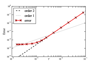
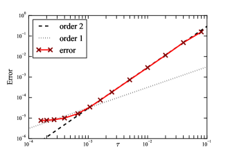
Figure 1: Error $\mathcal{E}(0.8)$ of the full discretization (10) plots for the problem with the damping coefficient $\gamma(t)=0$. Left: coarse space discretization ($328193$ degrees of freedom, $h=0.0139201$); Right: fine space discretization ($1311745$ degrees of freedom, $h=0.00697294$).

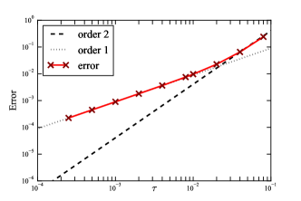
(a) vanilla IMEX scheme

(b) revised IMEX scheme

Figure 6: Error $\mathcal{E}(0.8)$ of the full discretization plots for the problem with the damping coefficient satisfying $r_{1}=r_{2}=1$ and $\eta=1$.

Regarding the damping coefficient $\gamma(t)=(1+t)^{-2}$, Figure 2 illustrates the temporal convergence rates of the full discretizations (10) and (12) for the fine space discretization ($h=0.00697294$). It can be observed that the scheme (10) converges with order one in terms of time step in Figure 2 (a), while the scheme (12) converges with order two in Figure 2 (b). The temporal convergence behaviors of both full discretizations for the problems with damping coefficients $\gamma(t)=1+t$, and $\gamma(t)=(1+t)^{2}$ are very similar to those in Figure 2, which can be seen clearly in Figure 6 and 7 of C.

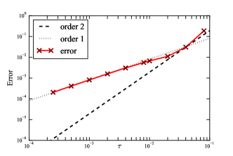
(a) vanilla IMEX scheme

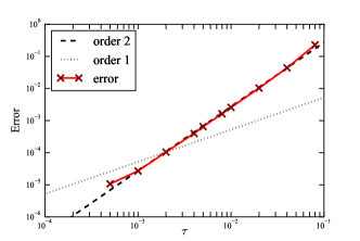
(b) revised IMEX scheme

Figure 2: Error $\mathcal{E}(0.8)$ of the full discretizations plots for the problem with the damping coefficient satisfying $r_{1}=r_{2}=1$ and $\eta=-2$.

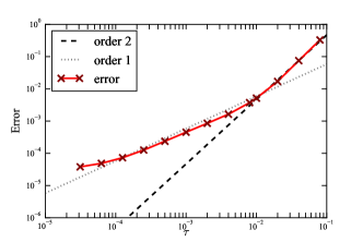
(a) Crank–Nicolson scheme

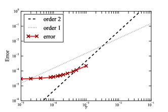
(b) Runge–Kutta scheme

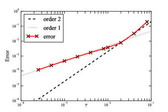
(c) vanilla IMEX scheme

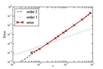
(d) revised IMEX scheme

Figure 3: Error $\mathcal{E}(0.8)$ of the full discretization plots for the problem with the damping coefficient satisfying $r_{1}=r_{2}=1$ and $\eta=-1$.

Finally, Figure 3 shows the errors of different time discrete schemes with the coarse spatial discretization ($h=0.0139201$) for the problem with the coefficient $\gamma(t)=(1+t)^{-1}$, while Figure 4 demonstrates a comparison of these errors pictured along the runtime. As can be seen easily, the Crank–Nicolson scheme (42) converges with order one (see Figure 3 (a)), but its convergence speed is much slower than that of of the revised IMEX scheme (18) as in Figure 4. It also indicates that the error of the scheme (12) reaches the space discretization error plateau fast compared to the scheme (10). Although the classical Runge–Kutta scheme [35] is more efficient than the revised IMEX scheme, the Runge–Kutta scheme is strictly restricted by time step (see Figure 3 (b)), which is only stable under a strong Courant–Friedrichs–Lewy condition. Additionally, Table 3 shows the execution time for various methods to achieve the same level of error, thereby highlighting the enhanced computational efficiency of our revised IMEX scheme.

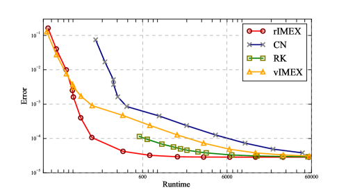
Figure 4: Error $\mathcal{E}(0.8)$ of different time schemes with the same space discretization ($h=0.0139201$) plotted against the runtime. Here, vIMEX: the vanilla IMEX scheme, rIMEX: the revised IMEX scheme, CN: the Crank–Nicolson scheme, and RK: the Runge–Kutta scheme.

Scheme	Runtime (s)
revised IMEX	$351.87$
vanilla IMEX	$6375.01$
RK	$2009.62$
CN	$21037.60$

Table 3: Runtime of the different schemes to reach the same error $\approx 4.6\times 10^{-5}$.

Example 2. The nonlinearities is chosen as

$$f_{1}(t,u)=|u|u,\quad f_{2}(t,u)=u^{3}$$

and the initial data is given by

$$u(0,x)=\left\{\begin{array}[]{cc}\cos^{2}\left(\pi|x|\right),&|x|\leqslant 0.5\\ 0,&\textrm{otherwise}\end{array}\right.,\quad\dot{u}(0,x)=0.$$

Figure 5 shows the propagation of the numerical solution by utilizing our revised IMEX scheme at various time points.

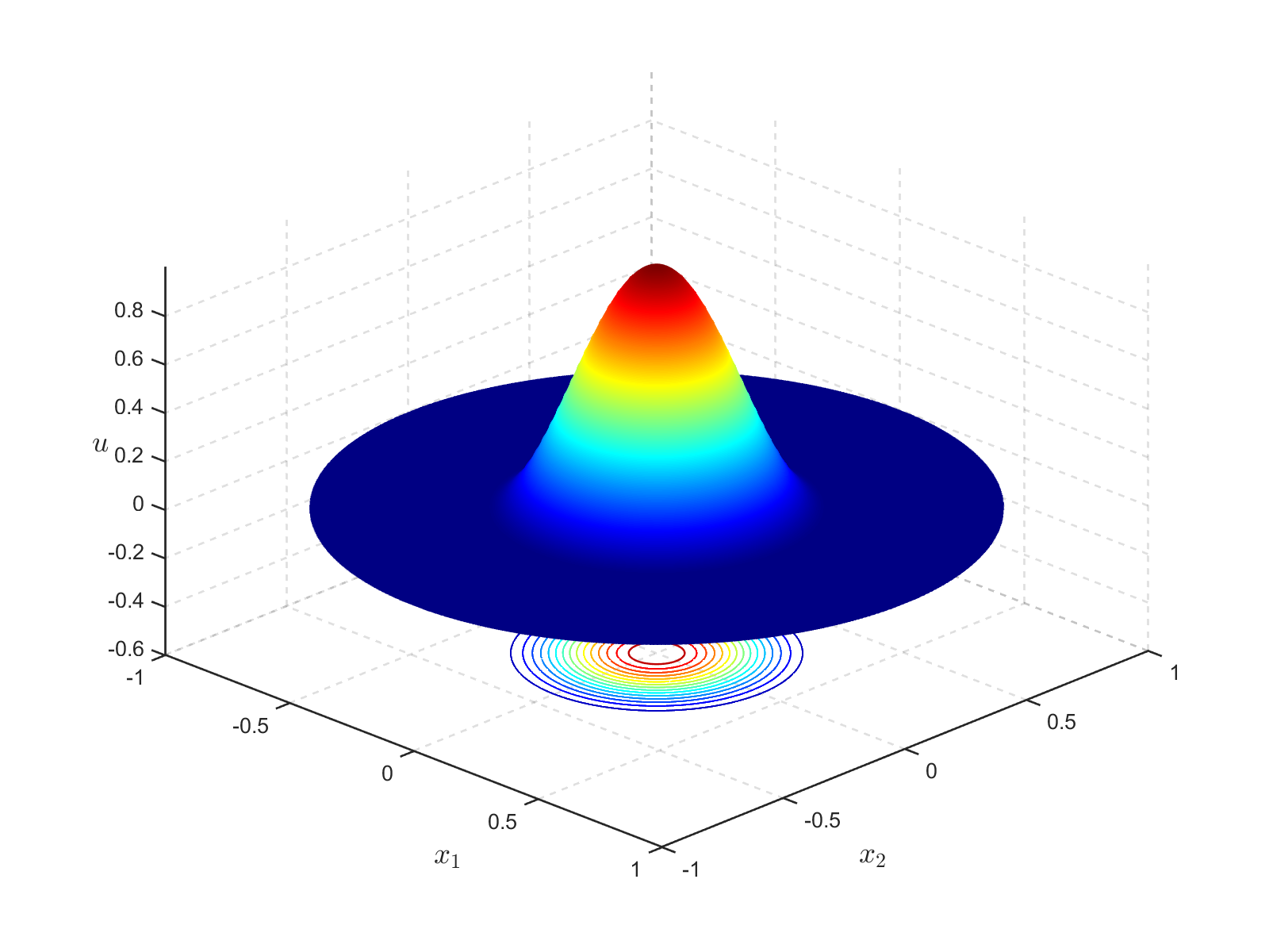
(a) $t=0$

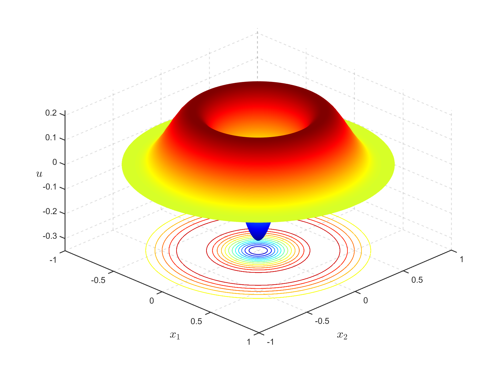
(b) $t=0.4$

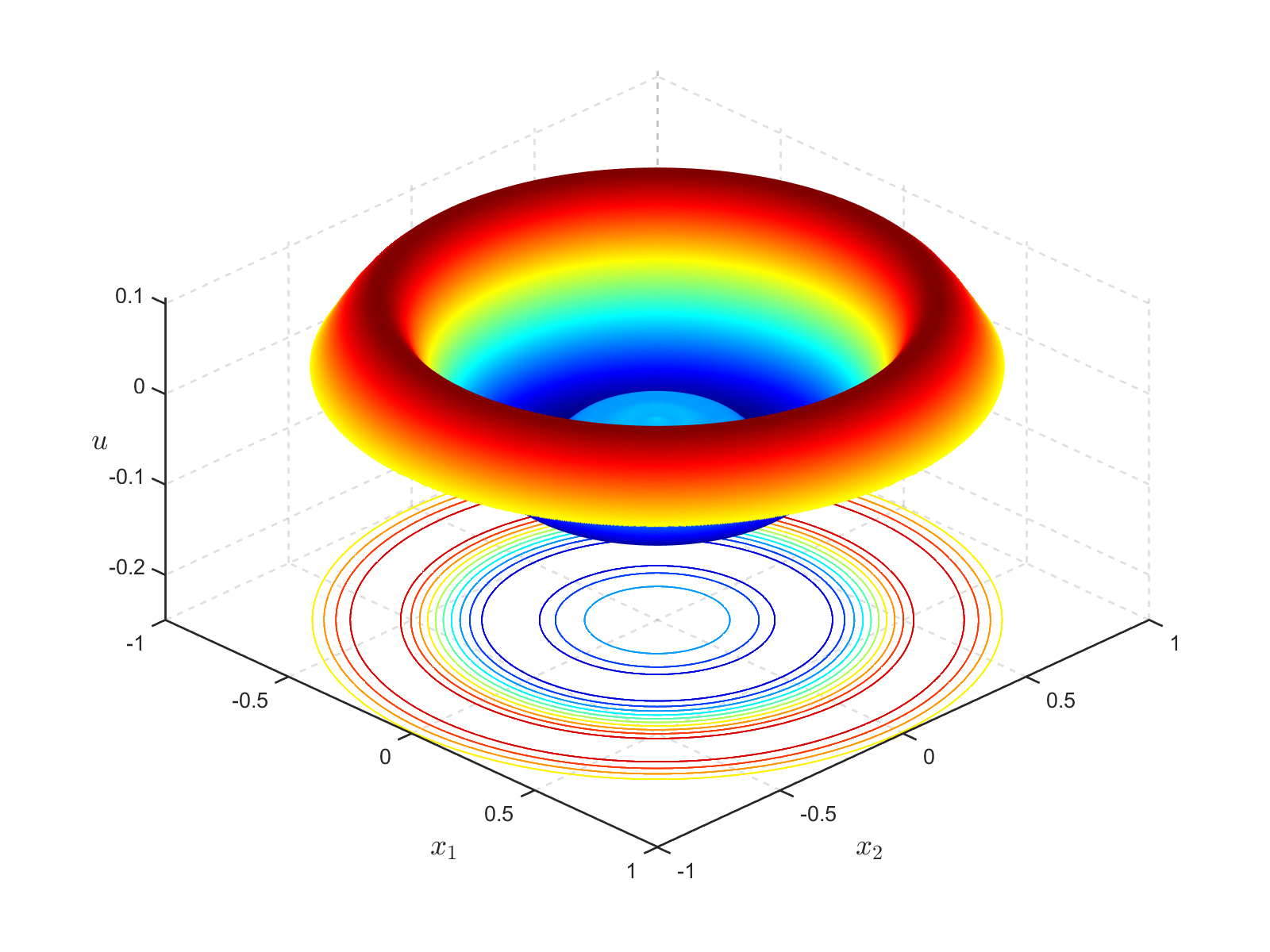
(c) $t=0.8$

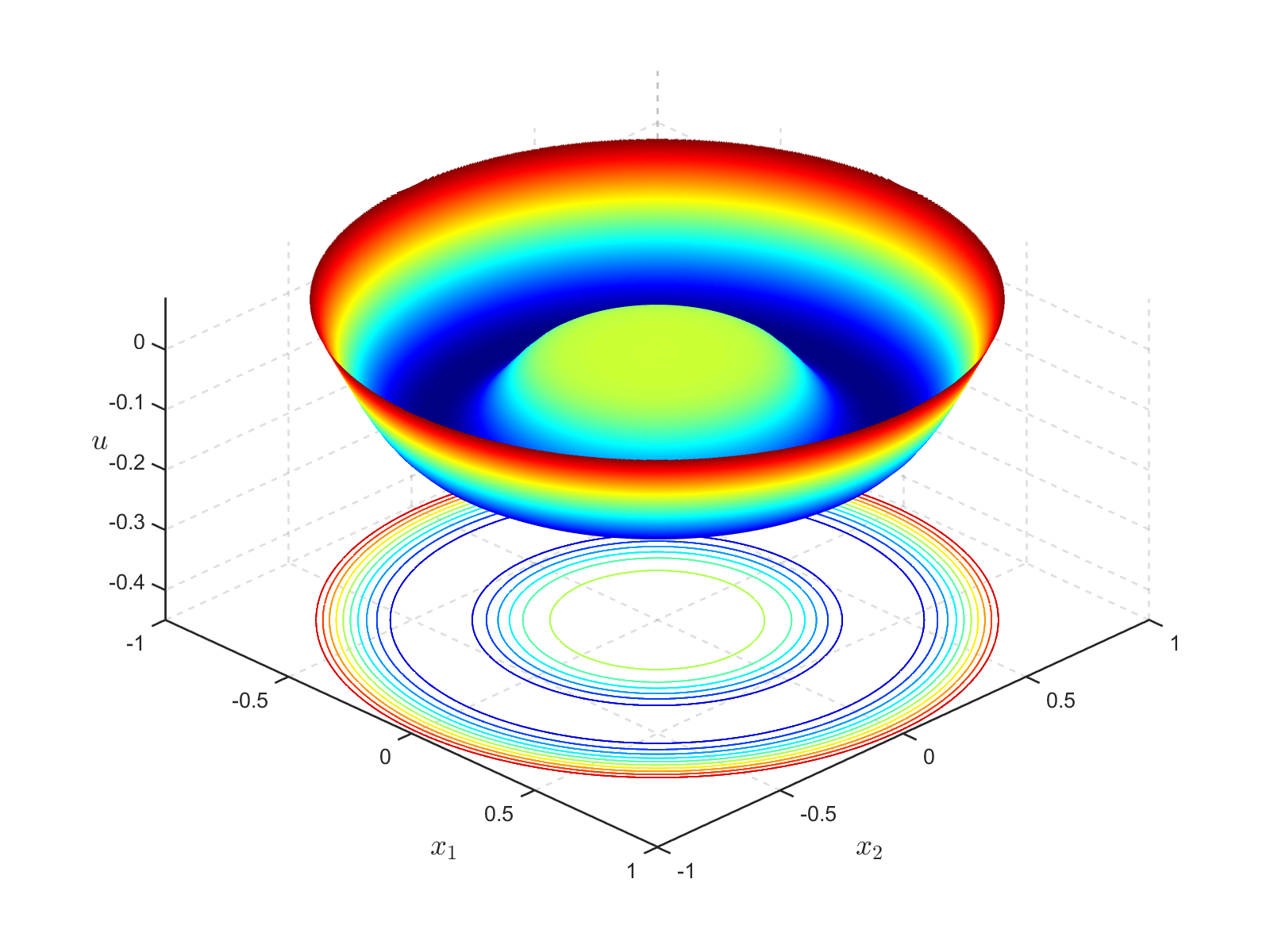
(d) $t=1.2$

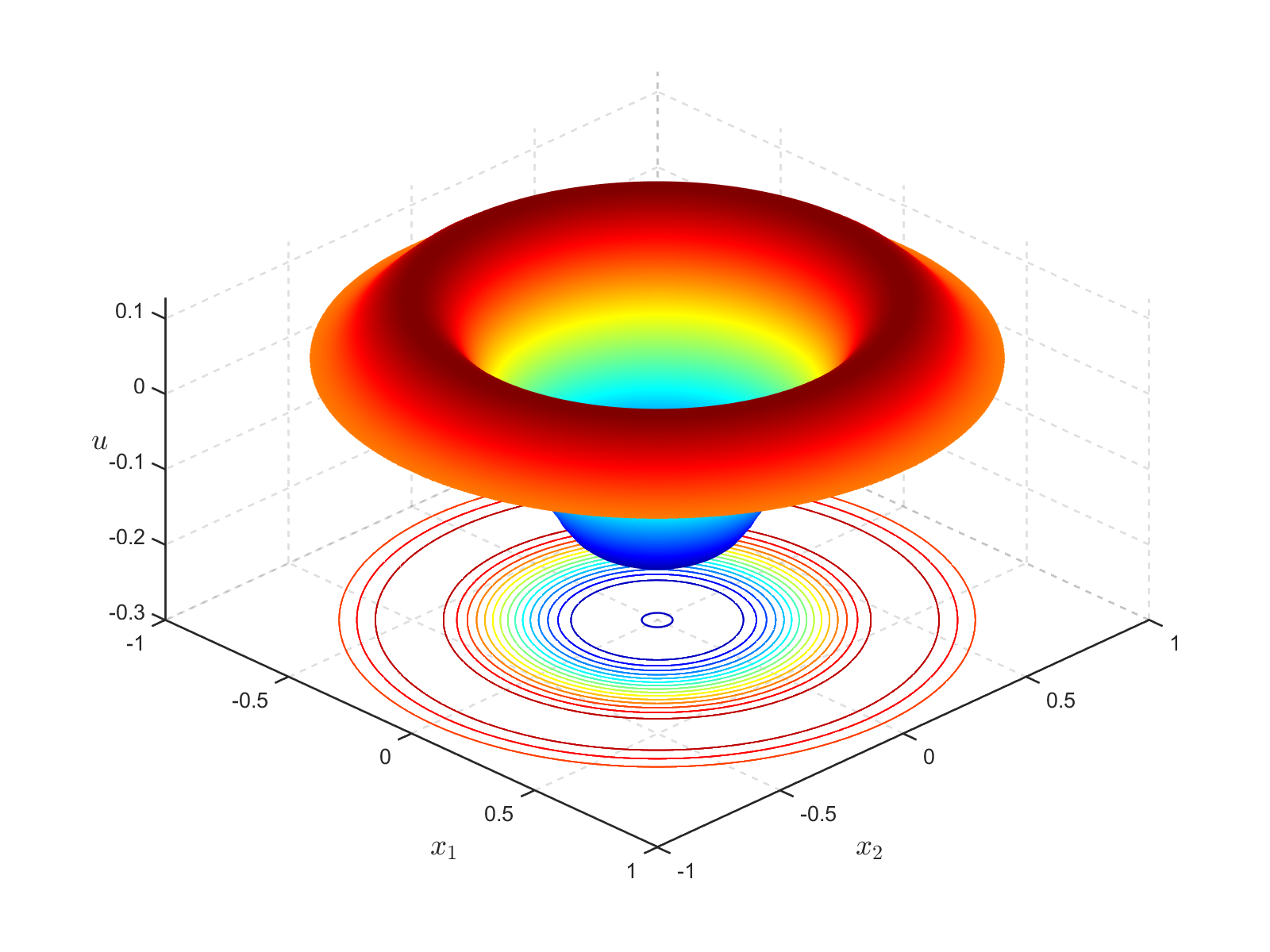
(e) $t=1.6$

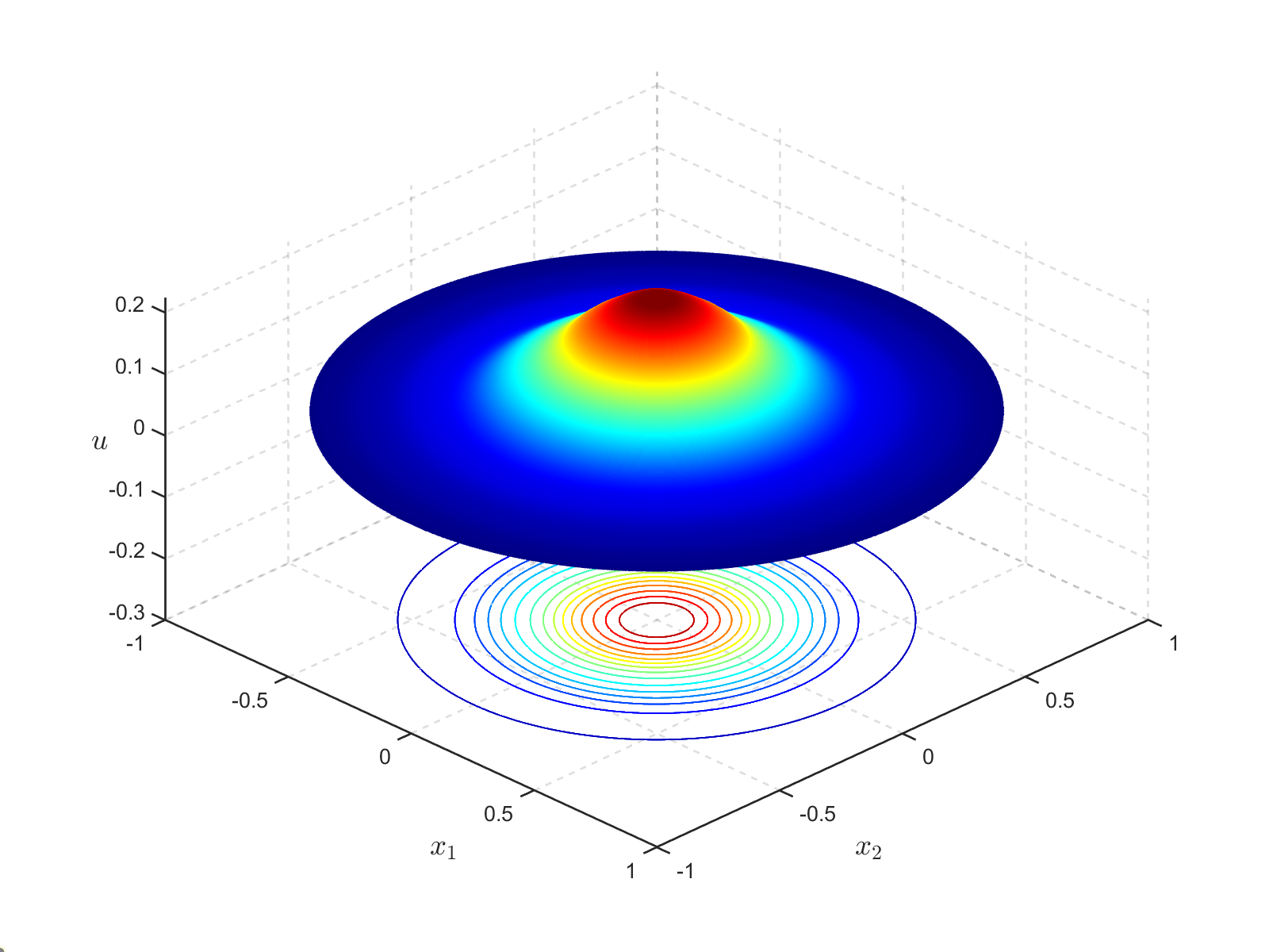
(f) $t=2.0$

Figure 5: The profiles of numerical solutions to the problem with the damping coefficient satisfying $r_{1}=r_{2}=1$ and $\eta=-1$.

Proof of Theorem 3.1

Using the similar idea (cf., e.g., [36, 32]) for error analysis, we give the proof of our main theorem. Throughout this section, $C_{1},C_{2},\cdots$ denote corresponding constants

Proof.

We use the notation $\mathbf{u}^{n}_{h}=[u^{n}_{h},v^{n}_{h}]^{\top}$ and $\tilde{\mathbf{u}}^{n}=[\tilde{u}^{n},\tilde{v}^{n}]^{\top}=[u(t_{n}),\dot{u}(t_{n})]^{\top}$ in the following. The subsequent proof consists of several steps.

Step 1. Note that the error of the scheme (10) can be split into two parts

$$\mathcal{L}_{h}\mathbf{u}^{n}_{h}-\mathbf{u}^{n}=\mathcal{L}_{h}(\mathbf{u}^{n}_{h}-\mathcal{J}_{h}\tilde{\mathbf{u}}^{n})+(\mathcal{L}_{h}\circ\mathcal{J}_{h}-I)\tilde{\mathbf{u}}^{n}$$

in which the operators $\mathcal{L}_{h}$ and $\mathcal{J}_{h}$ are given by

$$\mathcal{L}_{h}\mathbf{u}^{n}_{h}=\left[\begin{array}[]{c}\mathcal{L}^{V}_{h}u^{n}_{h}\\ \mathcal{L}^{V}_{h}v^{n}_{h}\end{array}\right],\quad\mathcal{J}_{h}\tilde{\mathbf{u}}^{n}=\left[\begin{array}[]{c}\mathcal{L}^{V^{\ast}}_{h}\tilde{u}^{n}\\ \mathcal{I}_{h}\tilde{v}^{n}\end{array}\right].$$

By using the triangle inequality we get

$$\begin{split}\|\mathcal{L}_{h}\mathbf{u}^{n}_{h}-\mathbf{u}^{n}\|_{X}&\leqslant\|\mathcal{L}_{h}(\mathbf{u}^{n}_{h}-\mathcal{J}_{h}\tilde{\mathbf{u}}^{n})\|_{X}+\|(\mathcal{L}_{h}\circ\mathcal{J}_{h}-I)\tilde{\mathbf{u}}^{n}\|_{X}\\ &\leqslant\max\{C_{\mathrm{H}},C_{\mathrm{V}}\}\|\mathbf{u}^{n}_{h}-\mathcal{J}_{h}\tilde{\mathbf{u}}^{n}\|_{X_{h}}+\|(\mathcal{L}_{h}\circ\mathcal{J}_{h}-I)\tilde{\mathbf{u}}^{n}\|_{X}.\end{split}$$ (19)

Step 2. Due to the following inequality

$$\small\begin{split}&\|(\mathcal{L}^{V^{\ast}}_{h}-\mathcal{I}_{h})\tilde{u}^{n}\|_{V_{h}}\\ &=\sup_{\|\omega_{h}\|_{V_{h}}=1}\mathrm{p}_{h}((\mathcal{L}^{V^{\ast}}_{h}-\mathcal{I}_{h})\tilde{u}^{n},\omega_{h})\\ &=\sup_{\|\omega_{h}\|_{V_{h}}=1}\left\{\mathrm{p}_{h}(\mathcal{L}^{V^{\ast}}_{h}\tilde{u}^{n},\omega_{h})-\mathrm{p}_{h}(\mathcal{I}_{h}\tilde{u}^{n},\omega_{h})\right\}\\ &=\sup_{\|\omega_{h}\|_{V_{h}}=1}\left\{\mathrm{p}(\tilde{u}^{n},\mathcal{L}^{V}_{h}\omega_{h})-\mathrm{p}(\mathcal{L}^{V}_{h}\circ\mathcal{I}_{h}\tilde{u}^{n},\mathcal{L}^{V}_{h}\omega_{h})+\mathrm{p}(\mathcal{L}^{V}_{h}\circ\mathcal{I}_{h}\tilde{u}^{n},\mathcal{L}^{V}_{h}\omega_{h})-\mathrm{p}_{h}(\mathcal{I}_{h}\tilde{u}^{n},\omega_{h})\right\}\\ &\leqslant\sup_{\|\omega_{h}\|_{V_{h}}=1}\left\{\mathrm{p}((I-\mathcal{L}^{V}_{h}\circ\mathcal{I}_{h})\tilde{u}^{n},\mathcal{L}^{V}_{h}\omega_{h})\right\}+\sup_{\|\omega_{h}\|_{V_{h}}=1}\left\{\mathrm{p}(\mathcal{L}^{V}_{h}\circ\mathcal{I}_{h}\tilde{u}^{n},\mathcal{L}^{V}_{h}\omega_{h})-\mathrm{p}_{h}(\mathcal{I}_{h}\tilde{u}^{n},\omega_{h})\right\}\\ &\leqslant C_{\mathrm{V}}\|(I-\mathcal{L}^{V}_{h}\circ\mathcal{I}_{h})\tilde{u}^{n}\|_{V}+\sup_{\|\omega_{h}\|_{V_{h}}=1}\left\{\mathrm{p}(\mathcal{L}^{V}_{h}\circ\mathcal{I}_{h}\tilde{u}^{n},\mathcal{L}^{V}_{h}\omega_{h})-\mathrm{p}_{h}(\mathcal{I}_{h}\tilde{u}^{n},\omega_{h})\right\}\\ &\leqslant C_{\mathrm{V}}\epsilon^{\mathrm{ip}}_{h}+\epsilon^{\mathrm{p}}_{h},\end{split}$$

we obtain

$$\begin{split}\|(\mathcal{L}_{h}\circ\mathcal{J}_{h}-I)\tilde{\mathbf{u}}^{n}\|_{X}&=\|(\mathcal{L}^{V}_{h}\circ\mathcal{L}^{V^{\ast}}_{h}-I)\tilde{u}^{n}\|_{V}+\|(\mathcal{L}^{V}_{h}\circ\mathcal{I}_{h}-I)\tilde{v}^{n}\|_{H}\\ &=\|(\mathcal{L}^{V}_{h}\circ\mathcal{L}^{V^{\ast}}_{h}-\mathcal{L}^{V}_{h}\circ\mathcal{I}_{h}+\mathcal{L}^{V}_{h}\circ\mathcal{I}_{h}-I)\tilde{u}^{n}\|_{V}+\|(\mathcal{L}^{V}_{h}\circ\mathcal{I}_{h}-I)\tilde{v}^{n}\|_{H}\\ &\leqslant\|\mathcal{L}^{V}_{h}(\mathcal{L}^{V^{\ast}}_{h}-\mathcal{I}_{h})\tilde{u}^{n}\|_{V}+\|(\mathcal{L}^{V}_{h}\circ\mathcal{I}_{h}-I)\tilde{u}^{n}\|_{V}+\|(\mathcal{L}^{V}_{h}\circ\mathcal{I}_{h}-I)\tilde{v}^{n}\|_{H}\\ &\leqslant C_{\mathrm{V}}\|(\mathcal{L}^{V^{\ast}}_{h}-\mathcal{I}_{h})\tilde{u}^{n}\|_{V_{h}}+\epsilon^{\mathrm{ip}}_{h}\\ &\leqslant C^{2}_{\mathrm{V}}\epsilon^{\mathrm{ip}}_{h}+C_{\mathrm{V}}\epsilon^{\mathrm{p}}_{h}+\epsilon^{\mathrm{ip}}_{h}\\ &\leqslant(1+C^{2}_{\mathrm{V}})\left\{\epsilon^{\mathrm{ip}}_{h}+\epsilon^{\mathrm{p}}_{h}\right\}.\end{split}$$ (20)

Step 3. Let $\mathbf{e}_{h}^{n}:=\mathbf{u}^{n}_{h}-\mathcal{J}_{h}\tilde{\mathbf{u}}^{n}$ denote the discrete error. We will derive the representation of $\mathbf{e}_{h}^{n}$.

The fully discrete scheme (10) can be rewritten as

$$\hat{P}_{+}\mathbf{u}_{h}^{n+1}=\hat{P}_{-}\mathbf{u}_{h}^{n}+\frac{\tau}{2}\left(g_{h}^{n}+g_{h}^{n+1}\right)+\frac{\tau^{2}}{4}\left[\begin{array}[]{c}f_{h}^{n}-f_{h}^{n+1}\\ -(B_{h}+\gamma^{n+1})\left(f_{h}^{n}-f_{h}^{n+1}\right)\end{array}\right]$$ (21)

with the discrete operators $\hat{P}_{\pm}=I\pm\frac{\tau}{2}S_{h}$ and $g_{h}^{n}=g_{h}(t_{n},\mathbf{u}_{h}^{n})$. Thanks to $\frac{\tau}{2}\left(\hat{\alpha}\frac{\hat{C}_{\mathrm{em}}}{2}+\hat{\beta}\right)<1$, the assertions that $\hat{P}_{+}$ is invertible holds true by [21, Lemma 2.14], (21) can be reformulated into

$$\mathbf{u}_{h}^{n+1}=\hat{P}\mathbf{u}_{h}^{n}+\frac{\tau}{2}\hat{P}^{-1}_{+}\left(g_{h}^{n}+g_{h}^{n+1}\right)+\frac{\tau^{2}}{4}\hat{P}^{-1}_{+}\left[\begin{array}[]{c}f_{h}^{n}-f_{h}^{n+1}\\ -(B_{h}+\gamma^{n+1})\left(f_{h}^{n}-f_{h}^{n+1}\right)\end{array}\right]$$ (22)

with $\hat{P}=\hat{P}^{-1}_{+}\hat{P}_{-}$.

Since the exact solution $\tilde{\mathbf{u}}(t)$ satisfies (3), we have

$$\frac{\tau}{2}(\dot{\tilde{\mathbf{u}}}^{n+1}+\dot{\tilde{\mathbf{u}}}^{n})=\frac{\tau}{2}\left(-S(\tilde{\mathbf{u}}^{n+1}+\tilde{\mathbf{u}}^{n})+\tilde{g}^{n+1}+\tilde{g}^{n}\right)$$

with $\tilde{g}^{n}=g(t_{n},\tilde{\mathbf{u}}^{n})$. By inserting $\tilde{\mathbf{u}}(t)$ into (40) we get

$$\tilde{\mathbf{u}}^{n+1}=\tilde{\mathbf{u}}^{n}+\frac{\tau}{2}\left(-S(\tilde{\mathbf{u}}^{n+1}+\tilde{\mathbf{u}}^{n})+\tilde{g}^{n}+\tilde{g}^{n+1}\right)-\Lambda^{n+1}$$ (23)

in which $\Lambda^{n+1}$ is a defect. Then this defect can be given by

$$\Lambda^{n+1}=\frac{\tau}{2}(\dot{\tilde{\mathbf{u}}}^{n+1}+\dot{\tilde{\mathbf{u}}}^{n})-(\tilde{\mathbf{u}}^{n+1}-\tilde{\mathbf{u}}^{n})=\frac{\tau}{2}(\dot{\tilde{\mathbf{u}}}^{n+1}+\dot{\tilde{\mathbf{u}}}^{n})+\int_{t_{n}}^{t_{n+1}}\dot{\tilde{\mathbf{u}}}(s)\mathrm{d}s.$$

Taking the operator $\mathcal{L}^{\ast}_{h}\left[\upsilon,\omega\right]^{\top}=\left[\mathcal{L}^{V^{\ast}}_{h}\upsilon,\mathcal{L}^{H^{\ast}}_{h}\omega\right]^{\top}$ on both sides of (23) yields

$$\mathcal{L}^{\ast}_{h}(\tilde{\mathbf{u}}^{n+1}-\tilde{\mathbf{u}}^{n})=\frac{\tau}{2}\left(-\mathcal{L}^{\ast}_{h}\circ S(\tilde{\mathbf{u}}^{n+1}+\tilde{\mathbf{u}}^{n})+\mathcal{L}^{\ast}_{h}\tilde{g}^{n}+\mathcal{L}^{\ast}_{h}\tilde{g}^{n+1}\right)-\mathcal{L}^{\ast}_{h}\Lambda^{n+1},$$

from which it deduces

$$\begin{split}&\mathcal{J}_{h}(\tilde{\mathbf{u}}^{n+1}-\tilde{\mathbf{u}}^{n})-(\mathcal{J}_{h}-\mathcal{L}^{\ast}_{h})(\tilde{\mathbf{u}}^{n+1}-\tilde{\mathbf{u}}^{n})\\ &=\frac{\tau}{2}\left(-S_{h}\circ\mathcal{J}_{h}(\tilde{\mathbf{u}}^{n+1}+\tilde{\mathbf{u}}^{n})+\tilde{g}_{h}^{n}+\tilde{g}_{h}^{n+1}\right)-\frac{\tau}{2}\left(-S_{h}\circ\mathcal{J}_{h}(\tilde{\mathbf{u}}^{n+1}+\tilde{\mathbf{u}}^{n})+\tilde{g}_{h}^{n}+\tilde{g}_{h}^{n+1}\right)\\ &\quad+\frac{\tau}{2}\left(-\mathcal{L}^{\ast}_{h}\circ S(\tilde{\mathbf{u}}^{n+1}+\tilde{\mathbf{u}}^{n})+\mathcal{L}^{\ast}_{h}\tilde{g}^{n}+\mathcal{L}^{\ast}_{h}\tilde{g}^{n+1}\right)-\mathcal{L}^{\ast}_{h}\Lambda^{n+1}\end{split}$$ (24)

with

$$\widetilde{g}^{n}_{h}=g^{n}_{h}(t_{n},\mathcal{J}_{h}\tilde{\mathbf{u}}^{n})=\left[\begin{array}[]{c}0\\ f_{h}(\mathcal{L}^{V^{\ast}}_{h}\tilde{u}^{n})-\gamma(t_{n})\mathcal{I}_{h}\tilde{v}^{n}\end{array}\right]=\left[\begin{array}[]{c}0\\ \tilde{f}^{n}_{h}-\gamma^{n}\mathcal{I}_{h}\tilde{v}^{n}\end{array}\right].$$

By setting

$$\small\begin{split}\Pi_{h}^{n+1}=(\mathcal{L}^{\ast}_{h}-\mathcal{J}_{h})(\tilde{\mathbf{u}}^{n+1}-\tilde{\mathbf{u}}^{n})+\frac{\tau}{2}(\mathcal{L}^{\ast}_{h}\circ S-S_{h}\circ\mathcal{J}_{h})(\tilde{\mathbf{u}}^{n+1}+\tilde{\mathbf{u}}^{n})-\frac{\tau}{2}(\mathcal{L}^{\ast}_{h}\tilde{g}^{n}-\tilde{g}_{h}^{n}+\mathcal{L}^{\ast}_{h}\tilde{g}^{n+1}-\tilde{g}_{h}^{n+1}),\end{split}$$

(24) can be expressed as

$$\mathcal{J}_{h}\tilde{\mathbf{u}}^{n+1}=\mathcal{J}_{h}\tilde{\mathbf{u}}^{n}+\frac{\tau}{2}\left(-S_{h}\circ\mathcal{J}_{h}(\tilde{\mathbf{u}}^{n+1}+\tilde{\mathbf{u}}^{n})+\tilde{g}_{h}^{n}+\tilde{g}_{h}^{n+1}\right)-\Pi_{h}^{n+1}-\mathcal{L}^{\ast}_{h}\Lambda^{n+1},$$

which is equivalent to the following representation

$$\mathcal{J}_{h}\tilde{\mathbf{u}}^{n+1}=\hat{P}\circ\mathcal{J}_{h}\tilde{\mathbf{u}}^{n}+\frac{\tau}{2}\hat{P}^{-1}_{+}\left(\tilde{g}_{h}^{n}+\tilde{g}_{h}^{n+1}\right)-\hat{P}^{-1}_{+}\Pi_{h}^{n+1}-\hat{P}^{-1}_{+}\mathcal{L}^{\ast}_{h}\Lambda^{n+1}.$$ (25)

Plugging $\mathcal{J}_{h}\tilde{\mathbf{u}}$ into (22) yields

$$\mathcal{J}_{h}\tilde{\mathbf{u}}^{n+1}=\hat{P}\circ\mathcal{J}_{h}\tilde{\mathbf{u}}^{n}+\frac{\tau}{2}\hat{P}^{-1}_{+}\left(\tilde{g}_{h}^{n}+\tilde{g}_{h}^{n+1}\right)+\frac{\tau^{2}}{4}\hat{P}^{-1}_{+}\left[\begin{array}[]{c}\tilde{f}_{h}^{n}-\tilde{f}_{h}^{n+1}\\ -(B_{h}+\gamma^{n+1})\left(\tilde{f}_{h}^{n}-\tilde{f}_{h}^{n+1}\right)\end{array}\right]-\Delta^{n+1}_{h}$$ (26)

with another defect $\Delta^{n+1}_{h}$. By comparing to (25), we get the

$$\Delta^{n+1}_{h}=\hat{P}^{-1}_{+}\Pi_{h}^{n+1}+\hat{P}^{-1}_{+}\mathcal{L}^{\ast}_{h}\Lambda^{n+1}+\Theta_{h}^{n+1},\quad\Theta_{h}^{n+1}=\frac{\tau^{2}}{4}\hat{P}^{-1}_{+}\left[\begin{array}[]{c}\tilde{f}_{h}^{n}-\tilde{f}_{h}^{n+1}\\ -(B_{h}+\gamma^{n+1})\left(\tilde{f}_{h}^{n}-\tilde{f}_{h}^{n+1}\right)\end{array}\right].$$

By subtracting (26) from (22) we obtain the following recursion

$$\small\mathbf{e}^{n+1}_{h}=\hat{P}\mathbf{e}^{n}_{h}+\frac{\tau}{2}\hat{P}^{-1}_{+}\left(g_{h}^{n}-\tilde{g}_{h}^{n}+g_{h}^{n+1}-\tilde{g}_{h}^{n+1}\right)+\frac{\tau^{2}}{4}\hat{P}^{-1}_{+}\left[\begin{array}[]{c}f_{h}^{n}-\tilde{f}_{h}^{n}-f_{h}^{n+1}+\tilde{f}_{h}^{n+1}\\ -(B_{h}+\gamma^{n+1})\left(f_{h}^{n}-\tilde{f}_{h}^{n}-f_{h}^{n+1}+\tilde{f}_{h}^{n+1}\right)\end{array}\right]-\Delta^{n+1}_{h},$$

which implies

$$\begin{split}\mathbf{e}^{n}_{h}&=\hat{P}^{n}\mathbf{e}^{0}_{h}+\sum_{m=1}^{n}\hat{P}^{n-m}\bigg{\{}\frac{\tau}{2}\hat{P}^{-1}_{+}\left(g_{h}^{m}-\tilde{g}_{h}^{m}+g_{h}^{m+1}-\tilde{g}_{h}^{m+1}\right)\\ &\quad+\frac{\tau^{2}}{4}\hat{P}^{-1}_{+}\left[\begin{array}[]{c}f_{h}^{m-1}-\tilde{f}_{h}^{m-1}-f_{h}^{m}+\tilde{f}_{h}^{m}\\ -(B_{h}+\gamma^{m+1})\left(f_{h}^{m-1}-\tilde{f}_{h}^{m-1}-f_{h}^{m}+\tilde{f}_{h}^{m}\right)\end{array}\right]-\Delta^{m}_{h}\bigg{\}}.\end{split}$$ (27)

Step 4. To bound $\|\mathbf{e}_{h}^{n}\|_{X_{h}}$, we need some preparations. By [21, Lemma 2.14] we know

$$\|\hat{P}\upsilon\|_{X_{h}}\leqslant e^{\tau\hat{c}_{0}}\|\upsilon\|_{X_{h}},\quad\|\hat{P}^{-1}_{+}\upsilon\|_{X_{h}}\leqslant\|\upsilon\|_{X_{h}},\quad\forall\upsilon\in X_{h}$$

with $\hat{c}_{0}=\hat{\alpha}\frac{\hat{C}_{\mathrm{em}}}{2}+\hat{\beta}$. Then we have

$$\begin{split}&\left\|\hat{P}^{n-m}\left\{\frac{\tau}{2}\hat{P}^{-1}_{+}\left(g_{h}^{m}-\tilde{g}_{h}^{m}+g_{h}^{m-1}-\tilde{g}_{h}^{m-1}\right)\right\}\right\|_{X_{h}}\\ &\leqslant\frac{\tau}{2}e^{(n-m)\tau\hat{c}_{0}}\left(\|\hat{P}^{-1}_{+}\left(g_{h}^{m}-\tilde{g}_{h}^{m}\right)\|_{X_{h}}+\|\hat{P}^{-1}_{+}\left(g_{h}^{m-1}-\tilde{g}_{h}^{m-1}\right)\|_{X_{h}}\right)\\ &\leqslant\frac{\tau}{2}e^{(n-m)\tau\hat{c}_{0}}\left(\|g_{h}^{m}-\tilde{g}_{h}^{m}\|_{X_{h}}+\|g_{h}^{m-1}-\tilde{g}_{h}^{m-1}\|_{X_{h}}\right).\end{split}$$ (28)

We note that $\|u^{m}_{h}\|_{V_{h}}\leqslant\delta$ and

$$\begin{split}\|\mathcal{L}^{V^{\ast}}_{h}\tilde{u}^{m}\|_{V_{h}}&=\sup_{\|\omega_{h}\|_{V_{h}}=1}\mathrm{p}_{h}(\mathcal{L}^{V^{\ast}}_{h}\tilde{u}^{m},\omega_{h})=\sup_{\|\omega_{h}\|_{V_{h}}=1}\mathrm{p}(\tilde{u}^{m},\mathcal{L}^{V}_{h}\omega_{h})\leqslant C_{\mathrm{V}}\|\tilde{u}^{m}\|_{V}\leqslant\delta.\end{split}$$

Then by using the Lipschitz-continuity of the discrete nonlinearity $f_{h}$ we have

$$\begin{split}\|g_{h}^{m}-\tilde{g}_{h}^{m}\|_{X_{h}}&=\left\|\left[\begin{array}[]{c}0\\ f_{h}(u^{m}_{h})-\gamma(t_{m})v^{m}_{h}-f_{h}(\mathcal{L}^{V^{\ast}}_{h}\tilde{u}^{m})+\gamma(t_{m})\mathcal{I}_{h}\tilde{v}^{m}\end{array}\right]\right\|_{X_{h}}\\ &\leqslant\left\|f_{h}(u^{m}_{h})-f_{h}(\mathcal{L}^{V^{\ast}}_{h}\tilde{u}^{m})\right\|_{H_{h}}+\gamma(t_{m})\left\|v^{m}_{h}-\mathcal{I}_{h}\tilde{v}^{m}\right\|_{H_{h}}\\ &\leqslant\hat{C}_{\delta}\|u^{m}_{h}-\mathcal{L}^{V^{\ast}}_{h}\tilde{u}^{m}\|_{V_{h}}+(\gamma_{0}+T)\|v^{m}_{h}-\mathcal{I}_{h}\tilde{v}^{m}\|_{H_{h}}\\ &\leqslant(\hat{C}_{\delta}+C_{\gamma})\|\mathbf{e}^{m}_{h}\|_{X_{h}}.\end{split}$$ (29)

Combing (28) and (29) gives

$$\begin{split}\left\|\hat{P}^{n-m}\left\{\frac{\tau}{2}\hat{P}^{-1}_{+}\left(g_{h}^{m}-\tilde{g}_{h}^{m}+g_{h}^{m-1}-\tilde{g}_{h}^{m-1}\right)\right\}\right\|_{X_{h}}\leqslant\frac{\tau}{2}(\hat{C}_{\delta}+C_{\gamma})e^{(n-m)\tau\hat{c}_{0}}\left(\|\mathbf{e}^{m}_{h}\|_{X_{h}}+\|\mathbf{e}^{m-1}_{h}\|_{X_{h}}\right).\end{split}$$ (30)

Let $\hat{Q}_{\pm}=I\pm\frac{\tau^{2}}{4}A_{h}\pm\frac{\tau}{2}B_{h}$. For $\frac{\tau^{2}}{2}\hat{\alpha}+\tau\hat{\beta}<1$ by [24, Lemma 4.6] we obtain $\hat{Q}_{+}$ is invertible and its inverse $\hat{Q}_{+}^{-1}$ satisfies

$$\|\hat{Q}_{+}^{-1}\upsilon\|_{V_{h}}\leqslant\frac{\sqrt{2}}{\tau}\|\upsilon\|_{H_{h}},\quad\|(-I+\hat{Q}_{+}^{-1})\upsilon\|_{H_{h}}\leqslant\|\upsilon\|_{H_{h}},\quad\|(-I+2\hat{Q}_{+}^{-1})\upsilon\|_{V_{h}}\leqslant e^{\frac{\tau^{2}}{2}\hat{\alpha}+\tau\hat{\beta}}\|\upsilon\|_{H_{h}}$$

for any $\upsilon\in H_{h}$. Furthermore, we can derive the representations of $\hat{P}^{-1}_{+}$ as

$$\hat{P}^{-1}_{+}=\left[\begin{array}[]{cc}\hat{Q}_{+}^{-1}(I+\frac{\tau}{2}B_{h})&\frac{\tau}{2}\hat{Q}_{+}^{-1}\\ -\frac{2}{\tau}+\frac{2}{\tau}\hat{Q}_{+}^{-1}(I+\frac{\tau}{2}B_{h})&\hat{Q}_{+}^{-1}\end{array}\right]$$

and

$$\begin{split}\hat{P}&=\hat{P}^{-1}_{+}\hat{P}_{-}=\hat{P}^{-1}_{+}(I-\frac{\tau}{2}S_{h})=\left[\begin{array}[]{cc}-I+\hat{Q}_{+}^{-1}(2I+B_{h})&\tau\hat{Q}_{+}^{-1}\\ -\frac{4}{\tau}+\frac{2}{\tau}\hat{Q}_{+}^{-1}(2I+\tau B_{h})&-I+2\hat{Q}_{+}^{-1}\end{array}\right].\end{split}$$

Thus, we have the estimates

$$\begin{split}\left\|\hat{P}^{-1}_{+}\left[\begin{array}[]{c}f_{h}^{m}-\tilde{f}_{h}^{m}\\ -B_{h}\left(f_{h}^{m}-\tilde{f}_{h}^{m}\right)\end{array}\right]\right\|_{X_{h}}&=\left\|\left[\begin{array}[]{c}\hat{Q}_{+}^{-1}(f_{h}^{m}-\tilde{f}_{h}^{m})\\ (-\frac{2}{\tau}+\frac{2}{\tau}\hat{Q}_{+}^{-1})\left(f_{h}^{m}-\tilde{f}_{h}^{m}\right)\end{array}\right]\right\|_{X_{h}}\\ &\leqslant\frac{\sqrt{2}}{\tau}\|f_{h}^{m}-\tilde{f}_{h}^{m}\|_{H_{h}}+\frac{2}{\tau}\|f_{h}^{m}-\tilde{f}_{h}^{m}\|_{H_{h}}\\ &\leqslant\frac{2\sqrt{3}}{\tau}\hat{C}_{\delta}\|\mathbf{e}^{m}_{h}\|_{X_{h}}\end{split}$$ (31)

and

$$\begin{split}\left\|\hat{P}^{-1}_{+}\left[\begin{array}[]{c}0\\ -\gamma^{m+1}\left(f_{h}^{m}-\tilde{f}_{h}^{m}\right)\end{array}\right]\right\|_{X_{h}}&=\left\|\gamma^{m+1}\left[\begin{array}[]{c}\frac{\tau}{2}\hat{Q}_{+}^{-1}(f_{h}^{m}-\tilde{f}_{h}^{m})\\ \hat{Q}_{+}^{-1}\left(f_{h}^{m}-\tilde{f}_{h}^{m}\right)\end{array}\right]\right\|_{X_{h}}\\ &\leqslant C_{\gamma}(\frac{\sqrt{2}}{2}+\frac{\sqrt{2}}{\tau})\hat{C}_{\delta}\|\mathbf{e}^{m}_{h}\|_{X_{h}}.\end{split}$$ (32)

Step 5. Taking the norm on (27), using the triangle inequality, (30), (31) and (32) gives

$$\begin{split}\left\|\mathbf{e}^{n}_{h}\right\|_{X_{h}}&\leqslant\left\|\hat{P}^{n}\mathbf{e}^{0}_{h}+\sum_{m=1}^{n}\hat{P}^{n-m}\Delta^{m}_{h}\right\|_{X_{h}}+\sum_{m=1}^{n}\left\|\hat{P}^{n-m}\bigg{\{}\frac{\tau}{2}\hat{P}^{-1}_{+}\left(g_{h}^{m}-\tilde{g}_{h}^{m}+g_{h}^{m+1}-\tilde{g}_{h}^{m+1}\right)\bigg{\}}\right\|_{X_{h}}\\ &\quad+\frac{\tau^{2}}{4}\sum_{m=1}^{n}\left\|\hat{P}^{n-m}\circ\hat{P}^{-1}_{+}\left[\begin{array}[]{c}f_{h}^{m-1}-\tilde{f}_{h}^{m-1}-f_{h}^{m}+\tilde{f}_{h}^{m}\\ -B_{h}\left(f_{h}^{m-1}-\tilde{f}_{h}^{m-1}-f_{h}^{m}+\tilde{f}_{h}^{m}\right)\end{array}\right]\right\|_{X_{h}}\\ &\quad+\frac{\tau^{2}}{4}\sum_{m=1}^{n}\left\|\hat{P}^{n-m}\circ\hat{P}^{-1}_{+}\left[\begin{array}[]{c}0\\ -\gamma^{m}\left(f_{h}^{m-1}-\tilde{f}_{h}^{m-1}-f_{h}^{m}+\tilde{f}_{h}^{m}\right)\end{array}\right]\right\|_{X_{h}}\\ &\leqslant\tau\hat{C}_{re}\sum_{m=1}^{n}e^{(n-m)\tau\hat{c}_{0}}\|\mathbf{e}^{m}_{h}\|_{X_{h}}+\left\|\hat{P}^{n}\mathbf{e}^{0}_{h}+\sum_{m=1}^{n}\hat{P}^{n-m}\Delta^{m}_{h}\right\|_{X_{h}}\end{split}$$

with $\hat{C}_{re}=(1+\sqrt{3})\hat{C}_{\delta}+C_{\gamma}+\frac{3\sqrt{2}}{4}\hat{C}_{\delta}C_{\gamma}$. Thanks to $\tau\hat{C}_{\mathrm{re}}<1$, we obtain

$$\begin{split}\left\|\mathbf{e}^{n}_{h}\right\|_{X_{h}}&\leqslant e^{\frac{n\tau\hat{C}_{re}}{1-\tau\hat{C}_{\mathrm{re}}}}\left\|\hat{P}^{n}\mathbf{e}^{0}_{h}+\sum_{m=1}^{n}\hat{P}^{n-m}\Delta^{m}_{h}\right\|_{X_{h}}\leqslant e^{\frac{n\tau\hat{C}_{re}}{1-\tau\hat{C}_{\mathrm{re}}}}\left(\left\|\hat{P}^{n}\mathbf{e}^{0}_{h}\right\|_{X_{h}}+\left\|\sum_{m=1}^{n}\hat{P}^{n-m}\Delta^{m}_{h}\right\|_{X_{h}}\right).\end{split}$$ (33)

by utilizing a discrete Gronwall inequality and the triangle inequality.

Due to

$$\small\begin{split}\left\|\Lambda^{m}\right\|_{X_{h}}=\left\|\tau^{3}\int_{0}^{1}\frac{s(1-s)}{2}\frac{\mathrm{d}^{3}}{\mathrm{d}t^{3}}\mathbf{u}(t_{m}+\tau s)\mathrm{d}s\right\|_{X_{h}}\leqslant\tau^{3}\left(\left\|\frac{\mathrm{d}^{4}u}{\mathrm{d}t^{4}}\right\|_{L^{\infty}([t_{m-1},t_{m}];H)}+\left\|\frac{\mathrm{d}^{3}u}{\mathrm{d}t^{3}}\right\|_{L^{\infty}([t_{m-1},t_{m}];V)}\right)\end{split}$$

and

$$\small\begin{split}\left\|\Pi_{h}^{m}\right\|_{X_{h}}&=\|(\mathcal{L}^{V^{\ast}}_{h}-\mathcal{I}_{h})(\tilde{v}^{m+1}-\tilde{v}^{m})\|_{H_{h}}+\frac{\tau}{2}\|(\mathcal{L}^{V^{\ast}}_{h}-\mathcal{I}_{h})(\tilde{v}^{m+1}+\tilde{v}^{m})\|_{V_{h}}\\ &\quad+\frac{\tau}{2}\left\|\mathcal{L}^{H^{\ast}}_{h}\left(A(\tilde{u}^{m+1}+\tilde{u}^{m})+B(\tilde{v}^{m+1}+\tilde{v}^{m})\right)-\left(A_{h}\mathcal{L}^{H^{\ast}}_{h}(\tilde{u}^{m+1}+\tilde{u}^{m})+B_{h}(\tilde{v}^{m+1}+\tilde{v}^{m})\mathcal{I}_{h}\right)\right\|_{H_{h}}\\ &\quad+\frac{\tau}{2}\left\|\mathcal{L}^{H^{\ast}}_{h}f(\tilde{u}^{m+1})-f_{h}(\mathcal{L}^{V^{\ast}}_{h}\tilde{u}^{m+1})\right\|_{H_{h}}+\frac{\tau}{2}\left\|\mathcal{L}^{H^{\ast}}_{h}f(\tilde{u}^{m})-f_{h}(\mathcal{L}^{V^{\ast}}_{h}\tilde{u}^{m})\right\|_{H_{h}}\\ &\quad+\gamma^{m}\frac{\tau}{2}\|(\mathcal{L}^{H^{\ast}}_{h}-\mathcal{I}_{h})(\tilde{v}^{m+1}+\tilde{v}^{m})\|_{H_{h}}\\ &\leqslant\tau(C_{\mathrm{V}}\epsilon^{\mathrm{ip}}_{h}+\epsilon^{\mathrm{p}}_{h})+\tau(C_{\mathrm{V}}\epsilon^{\mathrm{ip}}_{h}+\epsilon^{\mathrm{p}}_{h})+C\tau(\epsilon^{\mathrm{ip}}_{h}+\epsilon^{\mathrm{p}}_{h}+\epsilon^{\mathrm{b}}_{h})+\tau\epsilon^{\mathrm{data}}_{h}++\tau C_{\gamma}(C_{\mathrm{H}}\epsilon^{\mathrm{ip}}_{h}+\epsilon^{\mathrm{p}}_{h})\\ &\leqslant C_{1}\tau\epsilon^{\mathrm{total}}_{h},\end{split}$$

we have

$$\begin{split}\left\|\sum_{m=1}^{n}\hat{P}^{n-m}\Delta^{m}_{h}\right\|_{X_{h}}&=\left\|\sum_{m=1}^{n}\hat{P}^{n-m}\left(\hat{P}^{-1}_{+}\Pi_{h}^{m}+\hat{P}^{-1}_{+}\mathcal{L}^{\ast}_{h}\Lambda^{m}+\Theta_{h}^{m}\right)\right\|_{X_{h}}\\ &\leqslant\sum_{m=1}^{n}e^{(n-m)\tau\hat{c}_{0}}\left(\left\|\Pi_{h}^{m}\right\|_{X_{h}}+\max\{C_{\mathrm{H}},C_{\mathrm{V}}\}\left\|\Lambda^{m}\right\|_{X_{h}}\right)+\left\|\sum_{m=1}^{n}\hat{P}^{n-m}\Theta_{h}^{m}\right\|_{X_{h}}\\ &\leqslant C_{2}e^{n\tau\hat{c}_{0}}\left(\tau^{2}+\epsilon^{\mathrm{total}}_{h}\right)+\left\|\sum_{m=1}^{n}\hat{P}^{n-m}\Theta_{h}^{m}\right\|_{X_{h}}.\end{split}$$ (34)

It remains to bound the second term on the left hand side of (34). We set $\Theta_{h}^{m}=\Phi_{h}^{m}+\Psi_{h}^{m}$ with

$$\begin{split}\Phi_{h}^{m}=\frac{\tau^{2}}{4}\hat{P}^{-1}_{+}\left[\begin{array}[]{c}\tilde{f}_{h}^{m-1}-\tilde{f}_{h}^{m}\\ -B_{h}\left(\tilde{f}_{h}^{m-1}-\tilde{f}_{h}^{m}\right)\end{array}\right],\quad\Psi_{h}^{m}=\frac{\tau^{2}}{4}\hat{P}^{-1}_{+}\left[\begin{array}[]{c}0\\ -\gamma^{m}\left(\tilde{f}_{h}^{m-1}-\tilde{f}_{h}^{m}\right)\end{array}\right].\end{split}$$

We note that

$$\small\begin{split}\hat{Q}_{+}^{-1}\left(\tilde{f}_{h}^{m-1}-\tilde{f}_{h}^{m}\right)=\hat{Q}_{+}^{-1}\left(\tilde{f}_{h}^{m-1}-\mathcal{L}^{H^{\ast}}_{h}\tilde{f}^{m-1}-\tilde{f}_{h}^{m}+\mathcal{L}^{H^{\ast}}_{h}\tilde{f}^{m}\right)+\hat{Q}_{+}^{-1}\circ\mathcal{L}^{H^{\ast}}_{h}\left(\tilde{f}^{m-1}-\tilde{f}^{m}\right)\end{split}$$

and

$$\small\begin{split}&\left(-2+2\hat{Q}_{+}^{-1}\right)\left(-\mathcal{L}^{H^{\ast}}_{h}\tilde{f}^{m-1}+\mathcal{L}^{H^{\ast}}_{h}\tilde{f}^{m}\right)+\left(-I+2\hat{Q}_{+}^{-1}\right)\circ\mathcal{L}^{H^{\ast}}_{h}\left(\tilde{f}^{m-1}-\tilde{f}^{m}\right)-\mathcal{L}^{H^{\ast}}_{h}\left(\tilde{f}^{m-1}-\tilde{f}^{m}\right)\\ &=-2\hat{Q}_{+}^{-1}\circ\mathcal{L}^{H^{\ast}}_{h}\left(\tilde{f}^{m-1}-\tilde{f}^{m}\right)+\left(-I+2\hat{Q}_{+}^{-1}\right)\circ\mathcal{L}^{H^{\ast}}_{h}\left(\tilde{f}^{m-1}-\tilde{f}^{m}\right)+\mathcal{L}^{H^{\ast}}_{h}\left(\tilde{f}^{m-1}-\tilde{f}^{m}\right)\\ &=\left(-2\hat{Q}_{+}^{-1}+(-I+2\hat{Q}_{+}^{-1})\right)\mathcal{L}^{H^{\ast}}_{h}\left(\tilde{f}^{m-1}-\tilde{f}^{m}\right)+\mathcal{L}^{H^{\ast}}_{h}\left(\tilde{f}^{m-1}-\tilde{f}^{m}\right)\\ &=0.\end{split}$$

Then we have the following decomposition

$$\sum_{m=1}^{n}\hat{P}^{n-m}\Phi_{h}^{m}=\frac{\tau^{2}}{4}\sum_{m=1}^{n}\hat{P}^{n-m}\left[\begin{array}[]{c}\hat{Q}_{+}^{-1}\left(\tilde{f}_{h}^{m-1}-\tilde{f}_{h}^{m}\right)\\ (-\frac{2}{\tau}+\frac{2}{\tau}\hat{Q}_{+}^{-1})\left(\tilde{f}_{h}^{m-1}-\tilde{f}_{h}^{m}\right)\end{array}\right]=\sum_{m=1}^{n}\hat{P}^{n-m}\left(\Xi^{m}_{1}+\Xi^{m}_{2}+\Xi^{m}_{3}\right)$$ (35)

with

$$\Xi^{m}_{1}=\frac{\tau^{2}}{4}\left[\begin{array}[]{c}\hat{Q}_{+}^{-1}\left(\tilde{f}_{h}^{m-1}-\mathcal{L}^{H^{\ast}}_{h}\tilde{f}^{m-1}-\tilde{f}_{h}^{m}+\mathcal{L}^{H^{\ast}}_{h}\tilde{f}^{m}\right)\\ (-\frac{2}{\tau}+\frac{2}{\tau}\hat{Q}_{+}^{-1})\left(\tilde{f}_{h}^{m-1}-\mathcal{L}^{H^{\ast}}_{h}\tilde{f}^{m-1}-\tilde{f}_{h}^{m}+\mathcal{L}^{H^{\ast}}_{h}\tilde{f}^{m}\right)\end{array}\right]$$

and

$$\Xi^{m}_{2}=\frac{\tau}{4}\left[\begin{array}[]{c}\tau\hat{Q}_{+}^{-1}\circ\mathcal{L}^{H^{\ast}}_{h}\left(\tilde{f}^{m-1}-\tilde{f}^{m}\right)\\ (-I+2\hat{Q}_{+}^{-1})\circ\mathcal{L}^{H^{\ast}}_{h}\left(\tilde{f}^{m-1}-\tilde{f}^{m}\right)\end{array}\right],\quad\Xi^{m}_{3}=\frac{\tau}{4}\left[\begin{array}[]{c}0\\ -\mathcal{L}^{H^{\ast}}_{h}\left(\tilde{f}^{m-1}-\tilde{f}^{m}\right)\end{array}\right].$$

Since we have

$$\begin{split}\hat{P}\Xi^{m-1}_{3}=\left[\begin{array}[]{c}-\tau\hat{Q}_{+}^{-1}\mathcal{L}^{H^{\ast}}_{h}\left(\tilde{f}^{m-2}-\tilde{f}^{m-1}\right)\\ (I-2\hat{Q}_{+}^{-1})\circ\mathcal{L}^{H^{\ast}}_{h}\left(\tilde{f}^{m-2}-\tilde{f}^{m-1}\right)\end{array}\right]=-\Xi^{m-1}_{2},\end{split}$$

the decomposition (35) can be reformulated as

$$\begin{split}\sum_{m=1}^{n}\hat{P}^{n-m}\Phi_{h}^{m}&=\sum_{m=1}^{n}\hat{P}^{n-m}\Xi^{m}_{1}+\hat{P}^{n-1}\Xi^{1}_{2}+\sum_{m=2}^{n}\hat{P}^{n-m}\Xi^{m}_{2}+\sum_{m=1}^{n-1}\hat{P}^{n-m}\Xi^{m}_{3}+\Xi^{n}_{3}\\ &=\sum_{m=1}^{n}\hat{P}^{n-m}\Xi^{m}_{1}+\hat{P}^{n-1}\Xi^{1}_{2}+\sum_{m=2}^{n}\hat{P}^{n-m}\Xi^{m}_{2}+\sum_{m=2}^{n}\hat{P}^{n-m}(\hat{P}\Xi^{m-1}_{3})+\Xi^{n}_{3}\\ &=\sum_{m=1}^{n}\hat{P}^{n-m}\Xi^{m}_{1}+\hat{P}^{n-1}\Xi^{1}_{2}+\sum_{m=2}^{n}\hat{P}^{n-m}(\Xi^{m}_{2}-\Xi^{m-1}_{2})+\Xi^{n}_{3}.\end{split}$$ (36)

By the properties of $\hat{Q}_{+}^{-1}$ and $\mathcal{L}^{H^{\ast}}_{h}$, we have

$$\left\|\Xi^{m}_{1}\right\|_{X_{h}}\leqslant C_{3}\tau\epsilon^{\mathrm{data}}_{h},\quad\left\|\Xi^{1}_{2}\right\|_{X_{h}}\leqslant C_{4}\tau^{2},\quad\left\|\Xi^{n}_{3}\right\|_{X_{h}}\leqslant C_{5}\tau^{2}$$

and

$$\small\begin{split}\left\|\Xi^{m}_{2}-\Xi^{m-1}_{2}\right\|_{X_{h}}&=\frac{\tau}{4}\left\|\left[\begin{array}[]{c}\tau\hat{Q}_{+}^{-1}\circ\mathcal{L}^{H^{\ast}}_{h}\left(-\tilde{f}^{m-2}+2\tilde{f}^{m-1}-\tilde{f}^{m}\right)\\ (-I+2\hat{Q}_{+}^{-1})\circ\mathcal{L}^{H^{\ast}}_{h}\left(-\tilde{f}^{m-2}+2\tilde{f}^{m-1}-\tilde{f}^{m}\right)\end{array}\right]\right\|_{X_{h}}\\ &\leqslant C_{6}\tau\left\|-\tilde{f}^{m-2}+2\tilde{f}^{m-1}-\tilde{f}^{m}\right\|_{H}\\ &\leqslant C_{7}\tau^{3}\left\|\frac{\mathrm{d}^{2}}{\mathrm{d}t^{2}}f(u(t))\right\|_{L^{\infty}([t_{m-1},t_{m}];H)}\\ &=C_{7}\tau^{3}\left\|\frac{\mathrm{d}^{4}}{\mathrm{d}t^{4}}u(t)+A\left(\frac{\mathrm{d}^{2}}{\mathrm{d}t^{2}}u(t)\right)+B\left(\frac{\mathrm{d}^{3}}{\mathrm{d}t^{3}}u(t)\right)+\frac{\mathrm{d}^{2}}{\mathrm{d}t^{2}}\left(\gamma(t)u(t)\right)\right\|_{L^{\infty}([t_{m-1},t_{m}];H)}\\ &\leqslant(C_{8}+C_{\gamma})\tau^{3}\left(\left\|\frac{\mathrm{d}^{4}u}{\mathrm{d}t^{4}}\right\|_{L^{\infty}([t_{m-1},t_{m}];H)}+\left\|\frac{\mathrm{d}^{3}u}{\mathrm{d}t^{3}}\right\|_{L^{\infty}([t_{m-1},t_{m}];H)}+\left\|\ddot{u}\right\|_{L^{\infty}([t_{m-1},t_{m}];H)}+\left\|\ddot{u}\right\|_{L^{\infty}([t_{m-1},t_{m}];H)}\right).\end{split}$$

Taking the norm and inserting all the corresponding bounds into (36) give

$$\left\|\sum_{m=1}^{n}\hat{P}^{n-m}\Phi_{h}^{m}\right\|_{X_{h}}\leqslant C_{9}e^{n\tau\hat{c}_{0}}\left(\epsilon^{\mathrm{data}}_{h}+\tau^{2}\right).$$ (37)

By the following estimate

$$\begin{split}\left\|\Psi_{h}^{m}\right\|_{X_{h}}&=\frac{\tau^{2}}{4}\gamma^{m}\left\|\left[\begin{array}[]{c}\frac{\tau}{2}\hat{Q}_{+}^{-1}\left(\tilde{f}_{h}^{m-1}-\tilde{f}_{h}^{m}\right)\\ \hat{Q}_{+}^{-1}\left(\tilde{f}_{h}^{m-1}-\tilde{f}_{h}^{m}\right)\end{array}\right]\right\|_{X_{h}}\\ &\leqslant\frac{\tau^{2}}{4}(\frac{\sqrt{2}}{2}+\frac{\sqrt{2}}{\tau})C_{\gamma}\left\|\tilde{f}_{h}^{m-1}-\tilde{f}_{h}^{m}\right\|_{H_{h}}\\ &=\frac{\tau^{2}}{4}(\frac{\sqrt{2}}{2}+\frac{\sqrt{2}}{\tau})C_{\gamma}\left\|f_{h}(\mathcal{L}^{V^{\ast}}_{h}\tilde{u}^{m-1})-f_{h}(\mathcal{L}^{V^{\ast}}_{h}\tilde{u}^{m})\right\|_{H_{h}}\\ &\leqslant\frac{\tau^{2}}{4}(\frac{\sqrt{2}}{2}+\frac{\sqrt{2}}{\tau})C_{\gamma}\hat{C}_{\delta}C_{\mathrm{V}}\left\|u(t_{m-1})-u(t_{m})\right\|_{V}\\ &\leqslant\frac{\tau^{2}}{4}(\frac{\sqrt{2}}{2}\tau+\sqrt{2})C_{\gamma}\hat{C}_{\delta}C_{\mathrm{V}}\left\|\dot{u}\right\|_{L^{\infty}([t_{m-1},t_{m}];V)}\\ &\leqslant\frac{3\sqrt{2}\tau^{2}}{8}C_{\gamma}\hat{C}_{\delta}C_{\mathrm{V}}\left\|\dot{u}\right\|_{L^{\infty}([t_{m-1},t_{m}];V)}\end{split}$$

and setting $C_{10}=\frac{3\sqrt{2}}{8}\hat{C}_{\delta}C_{\mathrm{V}}\left\|\dot{u}\right\|_{L^{\infty}([t_{m-1},t_{m}];V)}$, we get

$$\left\|\sum_{m=1}^{n}\hat{P}^{n-m}\Psi_{h}^{m}\right\|_{X_{h}}\leqslant C_{10}C_{\gamma}e^{n\tau\hat{c}_{0}}\tau.$$ (38)

Inserting (34), (37), (38) and

$$\left\|\hat{P}^{n}\mathbf{e}^{0}_{h}\right\|_{X_{h}}\leqslant e^{n\tau\hat{c}_{0}}\left\|\mathbf{e}^{0}_{h}\right\|_{X_{h}}\leqslant e^{n\tau\hat{c}_{0}}\epsilon^{\mathrm{data}}_{h}$$

into (33) yields

$$\begin{split}\left\|\mathbf{e}^{n}_{h}\right\|_{X_{h}}&\leqslant\exp\left\{\frac{n\tau\hat{C}_{re}}{1-\tau\hat{C}_{\mathrm{re}}}\right\}\left(e^{n\tau\hat{c}_{0}}\epsilon^{\mathrm{data}}_{h}+C_{2}e^{n\tau\hat{c}_{0}}\left(\tau^{2}+\epsilon^{\mathrm{total}}_{h}\right)+C_{9}e^{n\tau\hat{c}_{0}}\left(\epsilon^{\mathrm{data}}_{h}+\tau^{2}\right)+C_{10}C_{\gamma}e^{n\tau\hat{c}_{0}}\tau\right)\\ &=C_{11}e^{Mn\tau}\left(\epsilon^{\mathrm{total}}_{h}+\tau^{2}+C_{\gamma}\tau\right)\end{split}$$ (39)

with $M=\frac{\hat{C}_{re}}{1-\tau\hat{C}_{\mathrm{re}}}+\hat{c}_{0}$.

Step 6. By (20) and (39), it deduce from (19) that

$$\|\mathcal{L}_{h}\mathbf{u}^{n}_{h}-\mathbf{u}^{n}\|_{X}\leqslant Ce^{Mn\tau}\left(\epsilon^{\mathrm{total}}_{h}+\tau^{2}+C_{\gamma}\tau\right).$$

Therefore, we complete the proof. ∎

Conclusions

In this paper, we have found from our theoretical results that one actually cannot expect $o(\tau^{2})$ convergence due to the effect of the nonautonomous damping. In numerical simulations, the reduced convergence rate can also be observed. Moreover, we have developed a revised IMEX scheme for the semilinear wave-type equations with time-varying dampings. Numerical tests are presented to substantiate the validity and efficiency of the revised numerical method. Notably, the numerical results confirms that the second order $o(\tau^{2})$ of the error can be reached.

Appendix A Crank-Nicolson scheme for Equation (3)

The Crank-Nicolson scheme for (3) is of the form

$$\mathbf{u}^{n+1}=\mathbf{u}^{n}+\frac{\tau}{2}\left(-S(\mathbf{u}^{n}+\mathbf{u}^{n+1})+g^{n}+g^{n+1}\right),$$ (40)

which can be written as

$$P_{+}\mathbf{u}^{n+1}=P_{-}\mathbf{u}^{n}+\frac{\tau}{2}\left(g^{n}+g^{n+1}\right)$$ (41)

with the operator $P_{\pm}=I\pm\frac{\tau}{2}S$ and $g^{n}=g(t_{n},\mathbf{u}^{n})$.

The two components of (40) have the form as follows.

$$u^{n+1} =u^{n}+\frac{\tau}{2}\left(v^{n}+v^{n+1}\right),$$

$$v^{n+1} =v^{n}-\frac{\tau}{2}A\left(u^{n}+u^{n+1}\right)-\frac{\tau}{2}B\left(v^{n}+v^{n+1}\right)-\frac{\tau}{2}\left(\gamma^{n}v^{n}+\gamma^{n+1}v^{n+1}\right)+\frac{\tau}{2}\left(f^{n}+f^{n+1}\right).$$

By $v^{n+\frac{1}{2}}:=\frac{1}{2}\left(v^{n}+v^{n+1}\right)$, we have

$$\begin{split}u^{n+1}&=u^{n}+\tau v^{n+\frac{1}{2}},\\ v^{n+1}&=v^{n}-\frac{\tau}{2}A\left(u^{n}+u^{n+1}\right)-\tau Bv^{n+\frac{1}{2}}-\tau\gamma^{n+1}v^{n+\frac{1}{2}}+\frac{\tau}{2}(\gamma^{n+1}-\gamma^{n})v^{n}+\frac{\tau}{2}\left(f^{n}+f^{n+1}\right).\end{split}$$

In the second equation, we eliminate $u^{n+1}$ using the first one and obtain

$$v^{n+1}=v^{n}-\tau Au^{n}-\frac{\tau^{2}}{2}Av^{n+\frac{1}{2}}-\tau Bv^{n+\frac{1}{2}}-\tau\gamma^{n+1}v^{n+\frac{1}{2}}+\frac{\tau}{2}(\gamma^{n+1}-\gamma^{n})v^{n}+\frac{\tau}{2}\left(f^{n}+f^{n+1}\right).$$

Finally, we can write (40) to be a half-full-half step formulation

$$\small\begin{split}v^{n+\frac{1}{2}}&=v^{n}-\frac{\tau}{2}Au^{n}-\frac{\tau^{2}}{4}Av^{n+\frac{1}{2}}-\frac{\tau}{2}Bv^{n+\frac{1}{2}}-\frac{\tau}{2}\gamma^{n+1}v^{n+\frac{1}{2}}+\frac{\tau}{4}(\gamma^{n+1}-\gamma^{n})v^{n}+\frac{\tau}{4}\left(f^{n}+f^{n+1}\right),\\ u^{n+1}&=u^{n}+\tau v^{n+\frac{1}{2}},\\ v^{n+1}&=v^{n+\frac{1}{2}}-\frac{\tau}{2}Au^{n}-\frac{\tau^{2}}{4}Av^{n+\frac{1}{2}}-\frac{\tau}{2}Bv^{n+\frac{1}{2}}-\frac{\tau}{2}\gamma^{n+1}v^{n+\frac{1}{2}}+\frac{\tau}{4}(\gamma^{n+1}-\gamma^{n})v^{n}+\frac{\tau}{4}\left(f^{n}+f^{n+1}\right).\end{split}$$ (42)

Appendix B vanilla IMEX scheme for Equation (3)

If we replace the trapezoidal rule for the nonlinearity in (42) by the left/right rectangular rule, respectively, we have the vanilla IMEX scheme as follows

$$v^{n+\frac{1}{2}} =v^{n}-\frac{\tau}{2}Au^{n}-\frac{\tau^{2}}{4}Av^{n+\frac{1}{2}}-\frac{\tau}{2}Bv^{n+\frac{1}{2}}-\frac{\tau}{2}\gamma^{n+1}v^{n+\frac{1}{2}}+\frac{\tau}{4}(\gamma^{n+1}-\gamma^{n})v^{n}+\frac{\tau}{2}f^{n},$$ (43)

$$u^{n+1} =u^{n}+\tau v^{n+\frac{1}{2}},$$ (44)

$$v^{n+1} =v^{n+\frac{1}{2}}-\frac{\tau}{2}Au^{n}-\frac{\tau^{2}}{4}Av^{n+\frac{1}{2}}-\frac{\tau}{2}Bv^{n+\frac{1}{2}}-\frac{\tau}{2}\gamma^{n+1}v^{n+\frac{1}{2}}+\frac{\tau}{4}(\gamma^{n+1}-\gamma^{n})v^{n}+\frac{\tau}{2}f^{n+1},$$ (45)

which can be regard as the combination of the Crank-Nicolson scheme for the linear part and the leapfrog scheme for the nonlinear part, respectively. This numerical scheme is developed in [32] for the first time.

The scheme (42) can be also reformulated as

$$P_{+}\mathbf{u}^{n+1}=P_{-}\mathbf{u}^{n}+\frac{\tau}{2}\left(g^{n}+g^{n+1}\right)+\frac{\tau^{2}}{4}\left[\begin{array}[]{c}f^{n}-f^{n+1}\\ -(B+\gamma^{n+1})\left(f^{n}-f^{n+1}\right)\end{array}\right].$$ (46)

Indeed, by subtracting (43) and (45) we have

$$v^{n+\frac{1}{2}}=\frac{1}{2}\left(v^{n}+v^{n+1}\right)+\frac{\tau}{4}\left(f^{n}-f^{n+1}\right).$$ (47)

Inserting (47) into (44) yields

$$u^{n+1}=u^{n}+\frac{\tau}{2}\left(v^{n}+v^{n+1}\right)+\frac{\tau^{2}}{4}\left(f^{n}-f^{n+1}\right).$$ (48)

By combing (43) with (45), and using (44) and (47) we get

$$\small\begin{split}v^{n+1}&=v^{n}-\tau Au^{n}-\frac{\tau^{2}}{2}Av^{n+\frac{1}{2}}-\tau Bv^{n+\frac{1}{2}}-\tau\gamma^{n+1}v^{n+\frac{1}{2}}+\frac{\tau}{2}(\gamma^{n+1}-\gamma^{n})v^{n}+\frac{\tau}{2}\left(f^{n}+f^{n+1}\right)\\ &=v^{n}-\tau Au^{n}-\frac{\tau}{2}A\left(u^{n+1}-u^{n}\right)-\tau Bv^{n+\frac{1}{2}}-\tau\gamma^{n+1}v^{n+\frac{1}{2}}+\frac{\tau}{2}(\gamma^{n+1}-\gamma^{n})v^{n}+\frac{\tau}{2}\left(f^{n}+f^{n+1}\right)\\ &=v^{n}-\frac{\tau}{2}A\left(u^{n+1}+u^{n}\right)-\tau Bv^{n+\frac{1}{2}}-\tau\gamma^{n+1}v^{n+\frac{1}{2}}+\frac{\tau}{2}(\gamma^{n+1}-\gamma^{n})v^{n}+\frac{\tau}{2}\left(f^{n}+f^{n+1}\right)\\ &=v^{n}-\frac{\tau}{2}A\left(u^{n+1}+u^{n}\right)-\frac{\tau}{2}B\left(v^{n}+v^{n+1}\right)-\frac{\tau}{2}\gamma^{n+1}\left(v^{n}+v^{n+1}\right)+\frac{\tau}{2}(\gamma^{n+1}-\gamma^{n})v^{n}+\frac{\tau}{2}\left(f^{n}+f^{n+1}\right)\\ &\quad-\frac{\tau^{2}}{4}B\left(f^{n}-f^{n+1}\right)-\frac{\tau^{2}}{4}\gamma^{n+1}\left(f^{n}-f^{n+1}\right)\\ \end{split}$$

which implies

$$\small\begin{split}v^{n+1}&=v^{n}-\frac{\tau}{2}A\left(u^{n+1}+u^{n}\right)-\frac{\tau}{2}B\left(v^{n}+v^{n+1}\right)\\ &\quad+\frac{\tau}{2}\left(f^{n}-\gamma^{n}v^{n}+f^{n+1}-\gamma^{n+1}v^{n+1}\right)-\frac{\tau^{2}}{4}(B+\gamma^{n+1})\left(f^{n}-f^{n+1}\right).\end{split}$$ (49)

Therefore, (48) and (49) are two components of (46).

Appendix C Numerical tests for different cases of $\gamma(t)$

In the following, we plot the errors of the vanilla IMEX, and the revised IMEX schemes with the fine spatial discretization ($h=0.00697294$) for the problem of Example 1 with another two damping coefficients.

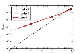
(a) vanilla IMEX scheme

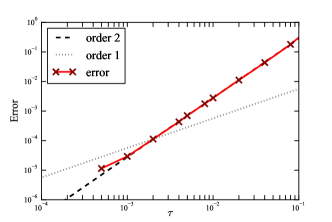
(b) revised IMEX scheme

Figure 7: Error $\mathcal{E}(0.8)$ of the full discretization plots for the problem with the damping coefficient satisfying $r_{1}=r_{2}=1$ and $\eta=2$.

Declaration of competing interest

The authors declare that they have no known competing financial interests or personal relationships that could have appeared to influence the work reported in this paper.

Data availability

Data sharing is not applicable to this article as no new data were created or analyzed in this study.

References

References

- [1] Miroslaw Kozlowski and Janina Marciak-Kozlowska. Thermal processes using attosecond laser pulses: When Time Matters, volume 121. Springer, 2006.
- [2] Allen T Chwang and Andy Chan. Interaction between porous media and wave motion. Annual Review of Fluid Mechanics, 30(1):53–84, 1998.
- [3] Michael S Howe. Acoustics of fluid-structure interactions. Cambridge university press, 1998.
- [4] Patrizia Pucci and James Serrin. Precise damping conditions for global asymptotic stability of second order systems. Acta Mathematica, 170(2):275–307, 1993.
- [5] Patrizia Pucci and James Serrin. Asymptotic stability for nonautonomous dissipative wave systems. Communications on Pure and Applied Mathematics, 49(2):177–216, 1996.
- [6] Bo Liu and Walter Littman. On the spectral properties and stabilization of acoustic flow. SIAM Journal on Applied Mathematics, 59(1):17–34, 1998.
- [7] Alexandre Cabot, Hans Engler, and Sébastien Gadat. On the long time behavior of second order differential equations with asymptotically small dissipation. Transactions of the American Mathematical Society, 361(11):5983–6017, 2009.
- [8] Enzo Vitillaro. Strong solutions for the wave equation with a kinetic boundary condition. Recent trends in nonlinear partial differential equations. I. Evolution problems, 594:295–307, 2013.
- [9] Delio Mugnolo and Enzo Vitillaro. The wave equation with acoustic boundary conditions on non-locally reacting surfaces. arXiv preprint arXiv:2105.09219, 2021.
- [10] Zhe Jiao, Yong Xu, and Lijing Zhao. Stability for nonlinear wave motions damped by time-dependent frictions. Communications in Nonlinear Science and Numerical Simulation, 117:106965, 2023.
- [11] Ibrahim Fatkullin and Jan S Hesthaven. Adaptive high-order finite-difference method for nonlinear wave problems. Journal of scientific computing, 16:47–67, 2001.
- [12] Dingwen Deng and Dong Liang. The energy-preserving finite difference methods and their analyses for system of nonlinear wave equations in two dimensions. Applied Numerical Mathematics, 151:172–198, 2020.
- [13] Lijian Jiang, Yalchin Efendiev, and Victor Ginting. Analysis of global multiscale finite element methods for wave equations with continuum spatial scales. Applied numerical mathematics, 60(8):862–876, 2010.
- [14] Mingyan He and Pengtao Sun. Energy-preserving finite element methods for a class of nonlinear wave equations. Applied Numerical Mathematics, 157:446–469, 2020.
- [15] Bruce Bukiet, John A Pelesko, Xiaolin Li, and Purushotham L Sachdev. A characteristic based numerical method with tracking for nonlinear wave equations. Computers & Mathematics with Applications, 31(7):75–99, 1996.
- [16] Kamrul Hasan, Humaira Takia, Muhammad Masudur Rahaman, Mehedi Hasan Sikdar, Bellal Hossain, and Khokon Hossen. Numerical study of the characteristics of shock and rarefaction waves for nonlinear wave equation. American Journal of Applied Scientific Research, 8(1):18–24, 2022.
- [17] Natalia Sternberg. A spectral method for nonlinear wave equations. Journal of Computational Physics, 72(2):422–434, 1987.
- [18] Bengt Fornberg and Tobin A Driscoll. A fast spectral algorithm for nonlinear wave equations with linear dispersion. Journal of Computational Physics, 155(2):456–467, 1999.
- [19] Philippe Saucez, A Vande Wouwer, WE Schiesser, and P Zegeling. Method of lines study of nonlinear dispersive waves. Journal of Computational and Applied Mathematics, 168(1-2):413–423, 2004.
- [20] Fatemeh Shakeri and Mehdi Dehghan. The method of lines for solution of the one-dimensional wave equation subject to an integral conservation condition. Computers & Mathematics with Applications, 56(9):2175–2188, 2008.
- [21] David Hipp. A unified error analysis for spatial discretizations of wave-type equations with applications to dynamic boundary conditions. PhD thesis, Karlsruher Institut für Technologie (KIT), 2017.
- [22] David Hipp, Marlis Hochbruck, and Christian Stohrer. Unified error analysis for nonconforming space discretizations of wave-type equations. IMA Journal of Numerical Analysis, 39(3):1206–1245, 2019.
- [23] Marlis Hochbruck and Jan Leibold. Finite element discretization of semilinear acoustic wave equations with kinetic boundary conditions. Electronic Transactions on Numerical Analysis, 53:522–540, 2020.
- [24] Jan Leibold. A unified error analysis for the numerical solution of nonlinear wave-type equations with application to kinetic boundary conditions. PhD thesis, Karlsruher Institut für Technologie (KIT), 2021.
- [25] Samet Y Kadioglu, Dana A Knoll, Robert B Lowrie, and Rick M Rauenzahn. A second order self-consistent imex method for radiation hydrodynamics. Journal of Computational Physics, 229(22):8313–8332, 2010.
- [26] Jean-François Lemieux, Dana A Knoll, Martin Losch, and Claude Girard. A second-order accurate in time implicit–explicit (imex) integration scheme for sea ice dynamics. Journal of Computational Physics, 263:375–392, 2014.
- [27] Georgios Akrivis. Stability of implicit-explicit backward difference formulas for nonlinear parabolic equations. SIAM Journal on Numerical Analysis, 53(1):464–484, 2015.
- [28] Yali Gao and Liquan Mei. Implicit–explicit multistep methods for general two-dimensional nonlinear schrödinger equations. Applied Numerical Mathematics, 109:41–60, 2016.
- [29] Uri M Ascher, Steven J Ruuth, and Raymond J Spiteri. Implicit-explicit runge-kutta methods for time-dependent partial differential equations. Applied Numerical Mathematics, 25(2-3):151–167, 1997.
- [30] Jason Frank, Willem Hundsdorfer, and Jan G Verwer. On the stability of implicit-explicit linear multistep methods. Applied Numerical Mathematics, 25(2-3):193–205, 1997.
- [31] William Layton, Yong Li, and Catalin Trenchea. Recent developments in imex methods with time filters for systems of evolution equations. Journal of Computational and Applied Mathematics, 299:50–67, 2016.
- [32] Marlis Hochbruck and Jan Leibold. An implicit–explicit time discretization scheme for second-order semilinear wave equations with application to dynamic boundary conditions. Numerische Mathematik, 147(4):869–899, 2021.
- [33] Amnon Pazy. Semigroups of linear operators and applications to partial differential equations, volume 44. Springer Science & Business Media, 2012.
- [34] Charles M Elliott and Thomas Ranner. Finite element analysis for a coupled bulk–surface partial differential equation. IMA Journal of Numerical Analysis, 33(2):377–402, 2013.
- [35] Eskil Hansen. Runge-kutta time discretizations of nonlinear dissipative evolution equations. Mathematics of computation, 75(254):631–640, 2006.
- [36] Marlis Hochbruck and Andreas Sturm. Error analysis of a second-order locally implicit method for linear maxwell’s equations. SIAM Journal on Numerical Analysis, 54(5):3167–3191, 2016.