Scaling-based Data Augmentation for Generative Models
and its Theoretical Extension

Yoshitaka Koike Science Tokyo  Takumi Nakagawa Science Tokyo/RIKEN  Hiroki Waida Science Tokyo  Takafumi Kanamori Science Tokyo/RIKEN. (kanamori@c.titech.ac.jp)
Abstract

This paper studies stable learning methods for generative models that enable high-quality data generation. Noise injection is commonly used to stabilize learning. However, selecting a suitable noise distribution is challenging. Diffusion-GAN, a recently developed method, addresses this by using the diffusion process with a timestep-dependent discriminator. We investigate Diffusion-GAN and reveal that data scaling is a key component for stable learning and high-quality data generation. Building on our findings, we propose a learning algorithm, Scale-GAN, that uses data scaling and variance-based regularization. Furthermore, we theoretically prove that data scaling controls the bias-variance trade-off of the estimation error bound. As a theoretical extension, we consider GAN with invertible data augmentations. Comparative evaluations on benchmark datasets demonstrate the effectiveness of our method in improving stability and accuracy.

1 Introduction

Generative adversarial networks (GANs) and their numerous variants can generate high-quality samples, such as images, audio, and graphs (Goodfellow et al.,, 2014; Arjovsky et al.,, 2017; Gulrajani et al.,, 2017; Mao et al.,, 2017; Radford et al.,, 2015; Miyato et al.,, 2018; Brock et al.,, 2018; Zhang et al.,, 2019; Li et al.,, 2017; Karras et al.,, 2019; Karras et al., 2020b, ; Karras et al.,, 2021; Sauer et al.,, 2021; Wang et al.,, 2023; Van Den Oord et al.,, 2016; De Cao and Kipf,, 2018). Although learning with diffusion models has received much attention in recent years (Ho et al.,, 2020; Song et al.,, 2020), generative models properly trained with GANs are still superior in terms of the quality and computation efficiency of data generation (Xiao et al.,, 2021; Sauer et al.,, 2022). However, GANs have stability issues that have not yet been fully resolved, such as lack of convergence, mode collapse, and catastrophic forgetting (Thanh-Tung and Tran,, 2020), in addition to overfitting, a common problem in machine learning.

Many studies have been conducted to alleviate these problems including modification of loss function, noise injection, adaptive instance normalization (Huang and Belongie,, 2017), weight normalization (Ioffe and Szegedy,, 2015; Ba et al.,, 2016; Wu and He,, 2018), Jacobian regularization (Mescheder et al.,, 2017; Nagarajan and Kolter,, 2017; Nie and Patel,, 2020), and utilization of pre-trained diffusion-models (Luo et al.,, 2024; Xia et al.,, 2024). To avoid overfitting, the regularization to the discriminator’s gradient is widely exploited (Arjovsky et al.,, 2017; Gulrajani et al.,, 2017; Miyato et al.,, 2018; Kodali et al.,, 2017; Adler and Lunz,, 2018; Petzka et al.,, 2018; Xu,, 2021; Mescheder et al.,, 2018; Zhou et al.,, 2019; Thanh-Tung et al.,, 2018). Details of related works are summarized in Section A.

Noise injection is another popular approach for stabilizing GANs (Roth et al.,, 2017). The instability occurs when the support of the distributions is far apart. By bringing the true training data and fake generated data closer together by noise injection, the discriminator’s overfitting can be alleviated. As summarized in Section A.2, Diffusion-GAN (Wang et al.,, 2023), inspired by the Denoising Diffusion Probabilistic Model (DDPM) (Ho et al.,, 2020; Song et al.,, 2020), showed that the addition of noise contributes to stable learning and improves accuracy for GAN. As DDPM does, Diffusion-GAN diffuses the data by scaling toward the origin and noise injection, i.e., diffusion process. Furthermore, the strength of the data scaling is adaptively updated according to the degree of overfitting of the discriminator. While this strategy is powerful as a learning stabilization, it is unclear which component in Diffusion-GAN contributes to improving the data generation performance. Besides the diffusion-GAN, the fusion of GANs and diffusion models have been considered to improve the efficiency, speed, and quality of generative models Zheng et al., (2022); Yin et al., 2024b ; Sauer et al., (2023); Kim et al., (2023); Yin et al., 2024a .

This paper studies stable learning methods for generative models.For that purpose, we deconstruct the components of Diffusion-GAN and analyze the significance of each. We conduct numerical simulations to identify critical factors for stable learning and high-quality sampling. We also investigate regularization to stabilize the learning process. Using the findings from the above discussion, we propose the learning algorithm called Scale-GAN, which uses data scaling and variance-based regularization. Our empirical studies on benchmark datasets in image generation demonstrate that the proposed method performs superior to existing methods. The contributions of this paper are summarized below.

  • We reveal that data scaling contributes more significantly to stabilization than noise injection. Indeed, data scaling helps avoid mode collapse. Compared to data scaling without noise injection, the data diffusion with noise makes it harder for the discriminator to convey an effective gradient direction to the generator.

  • In GAN-based learning methods, the discrepancy between true training data and fake generated data, and the discriminator’s gradient, is often incorporated into the loss function. We introduce a regularization method that leverages the discriminator’s variance as an approximation of the regularization for the gradient, offering a simpler yet effective approach.

  • We analyze theoretical properties of the proposed method, including i) the invariance of gradient direction to the scaling intensity, ii) the influence of the variance-based regularization on the generator’s distribution, and iii) the relationship between the scaling strategy and the generalization performance.

2 A Brief Survey of Diffusion-GAN

Diffusion-GAN (Wang et al.,, 2023) is a learning method for generative models inspired by the success of diffusion models and revisits the use of instance noise in GANs. Similar to vanilla GAN (Goodfellow et al.,, 2014), the learning of Diffusion-GAN is formulated as the following min-max optimization problem,

$\displaystyle\min_{\theta}\max_{\phi}\mathbb{E}_{{\bm{x}},t}\mathbb{E}_{{\bm{y}}}[\,\log(D_{\phi}(\boldsymbol{y},t))\mid{\bm{x}},t\,]+\mathbb{E}_{{\bm{z}},t}\mathbb{E}_{{\bm{y}}}[\,\log(1-D_{\phi}(\boldsymbol{y},t))\mid G_{\theta}({\bm{z}}),t\,],$

where $G_{\theta}$ is a generator and $D_{\phi}$ is a discriminator depending on the scaling intensity $t$. Differently from the vanilla GAN, both training and generated samples are diffused with a conditional multivariate normal distribution $\mathcal{N}\left(\boldsymbol{y};s_{t}\boldsymbol{x},(1-s_{t}^{2})\sigma^{2}\boldsymbol{I}\right)$ with mean $s_{t}\boldsymbol{x}$ and the variance-covariance matrix $(1-s_{t}^{2})\sigma^{2}\boldsymbol{I}$, The scaling function $s_{t}$ determines the diffusion schedule, and various scheduling schemes have been devised for the diffusion model. As the distribution of the scaling intensity $t$, the uniform distribution $\pi(t)=1/T$, or the priority distribution $\pi(t)\propto t$ for $t\in\{0,1,\ldots,T\}$ is often used. In practice, a fixed $T$ is not recommended. Instead, Karras et al., 2020a and Wang et al., (2023) proposed an adaptive update rule for $T$ according to how much the discriminator overfits to the training data.

As shown above, Diffusion-GAN consists of three main components: i) data scaling, ii) noise injection, and iii) scaling strategy consisting of $s_{t}$ and $\pi(t)$. In Section 3, we deconstruct each component of Diffusion-GAN and analyze how each contributes to learning stability and data-generation quality.

3 Data Scaling and Noise Injection

The simulation setting is the following. Suppose that i.i.d. samples, ${{\bm{x}}}_{1},\ldots,{{\bm{x}}}_{n},n=80$, are generated from the two-dimensional Gaussian mixture distribution with eight components, $\sum_{k=1}^{8}\frac{1}{8}\mathcal{N}({\bm{\mu}}_{k},\sigma^{2}I_{2})$, where ${\bm{\mu}}_{k}=(\cos(2\pi k/8),\sin(2\pi k/8)),k=1,\ldots,8$ and $\sigma^{2}=0.05$. Four-layer fully connected neural networks with LeakyReLU activation function are used for the discriminator and generator. The LeakyReLU is used in StyleGAN2 (Karras et al., 2020b, ). The findings in this section will also be confirmed for the standard benchmark datasets in Section 5.

3.1 Data Scaling

We investigate the effect of the data scaling. Scale the data by $s=0.25,0.5,1,1.5$ respectively, and train the scaled generator $sG_{\theta}$ and the discriminator $D_{\phi}$ having the learning parameters $\theta$ and $\phi$ using the scaled data $\{{\bm{y}}_{i}\}_{i=1}^{80}$ for ${\bm{y}}_{i}=s{\bm{x}}_{i}$. Since applying data scaling only to the training data causes a bias in the generator, it also applies to the generated data, which has been studied by Wang et al., (2023); Jenni and Favaro, (2019); Tran et al., (2021); Zhao et al., (2020); Karras et al., 2020a . The data scaling does not apply to $D_{\phi}$.

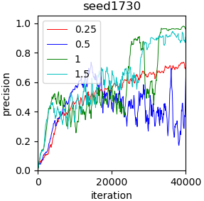
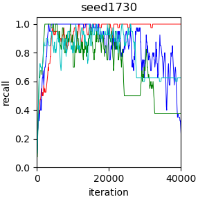
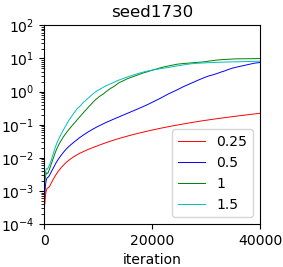
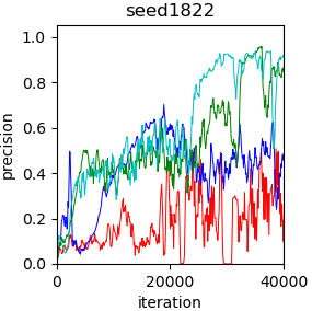
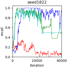
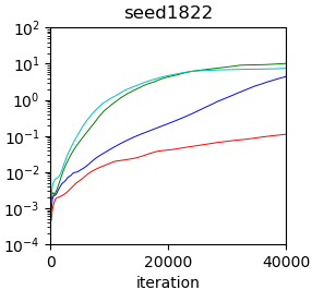
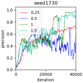
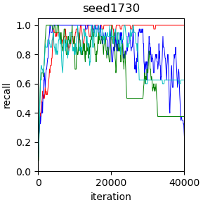
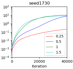
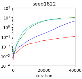
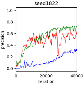
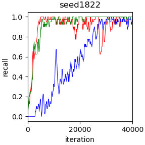
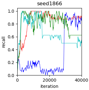
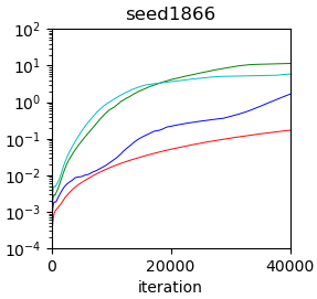
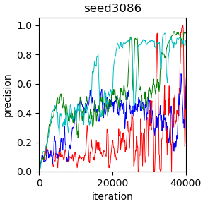
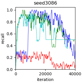
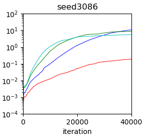
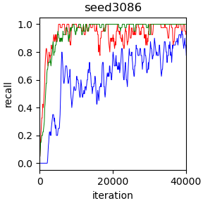
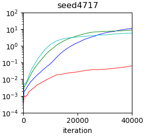
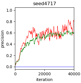
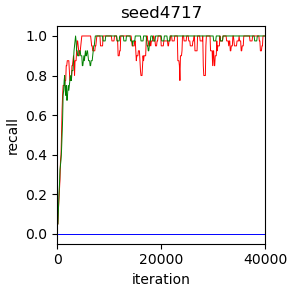
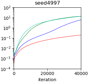
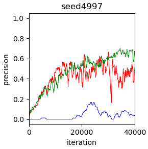
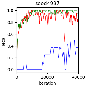
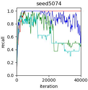
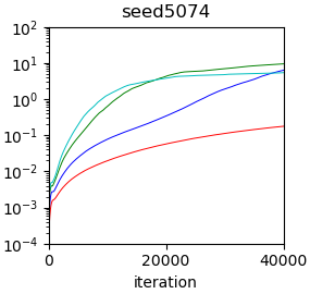
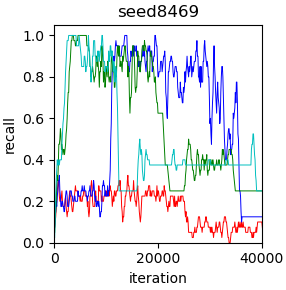
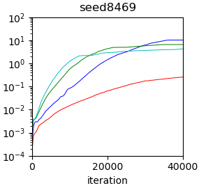
In Fig 1, (a) and (b) show precision and recall to training iterations for each scaling. Additional results with different seeds are reported in Section B. The learning with $s=0.25$ shows that if the data distribution is well covered by the generator, i.e., high recall is attained in the early stages of learning, the precision gradually increases, and the learning is successful. As shown in the lower panels of Fig 1, however, it has not escaped from the initial learning failure. These results can be explained by the size of the gradient for the discriminator, as shown in Fig 1 (c). The gradient norm for $s=0.25$ is smaller than the other cases, meaning that abrupt changes in the discriminator rarely occur. Hence, the learning result will be significantly affected by the early stages of the learning process. On the other hand, for $s=1,1.5$, high recall is achieved in the early stages of learning. However, it is observed that the recall drops significantly from the middle to the latter half of the learning period, causing mode collapse. Existing studies (Gulrajani et al.,, 2017; Kodali et al.,, 2017; Adler and Lunz,, 2018; Petzka et al.,, 2018; Xu,, 2021; Mescheder et al.,, 2018; Zhou et al.,, 2019; Thanh-Tung et al.,, 2018) have shown that a large gradient of the discriminator tends to cause instability.

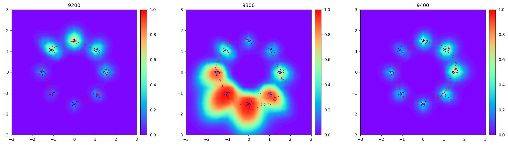
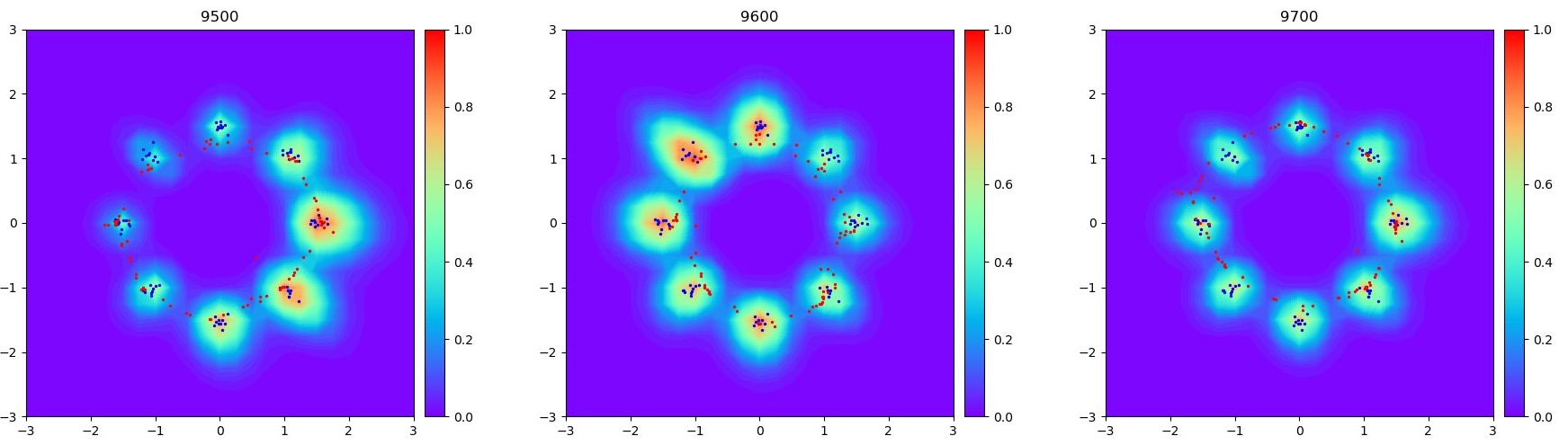
Fig 2, which visualizes the discriminator’s output at $s=1.5$, illustrates an unstable situation as the mode oscillates to higher predicted values at each iteration. This phenomenon is a precursor to mode decay. This oscillation leads to mode decay, known as catastrophic forgetting. We observed that the mode collapses occur even for $s=1.0$.

In summary, data scaling has a significant impact on learning dynamics. When the scale is small, the discriminator is less prone to sudden gradients and instability but is susceptible to early status in learning. Conversely, large scales make it easier to learn discriminant boundaries but are prone to instability before generating accurate samples. These results suggest that learning data at several scales simultaneously can reflect the good characteristics of each.

Refer to caption Refer to caption Refer to caption
(a) precision
(b) recall
(c) gradient norm
Figure 1: For each data scaling, (a) precision, (b) recall, and (c) averaged norm of discriminator’s gradient are depicted. The upper and lower panels correspond to two different seeds.
Refer to caption
Refer to caption
Figure 2: The discriminator’s predictions for $s=1.5$. The number of repetitions ranges from 9200 to 9700 from top left to bottom right. Blue (resp. Red) dots represent the data (resp. generated samples). Modes with high values change in an oscillatory manner, and the oscillations become more intense, leading to mode collapse.
Refer to caption Refer to caption
(a) precision (b) recall
Figure 3: (a) precision, and (b) recall for each scaling strategy, “fix”, “linear const”, and “adaptive”.

3.2 Scaling Strategy

Let us consider learning at multiple scales simultaneously. In a similar way as Ho et al., (2020), we define the scaling function $s_{t}$ by $s_{0}=1$ and $s_{t}=s_{t-1}\sqrt{1-\beta_{0}(1-t/T)-\beta_{T}t/T}$ for $t\in\{1,\ldots,T\}$. The parameters $\beta_{0}$ and $\beta_{T}$ control the decay rate and the scale at $T$. The distribution $\pi(t)$ of $t$ is given by $\pi(t)=\frac{1}{2}\pi_{0}(t)+\frac{1}{2}\delta_{0}(t)$, where $\delta_{0}$ is the point mass distribution at $t=0$, and $\pi_{0}$ is a pre-defined distribution on $\{1,\ldots,T\}$. Determine the distribution $\pi_{0}$ in three different ways and compare the properties of each;

  • i)

    $T$ is fixed to $T_{\max}$ and $\pi_{0}$ is the uniform distribution on $\{1,\ldots,T_{\max}\}$ (denoted by “fix”).

  • ii)

    $T$ increases in proportion to the learning iteration $i$ and make it constant from the middle (denoted by “linear const”), i.e., $\pi_{0}$ is the uniform distribution on $\{1,\ldots,T(i)\}$ with $T(i)=\min\left(\frac{2T_{\text{max}}}{I}i,T_{\text{max}}\right)$.

  • iii)

    $T$ adaptively changes by the following update rule, $T\leftarrow T+\operatorname{sign}(r_{d}-d_{\text{target }})$, for $r_{d}=\mathbb{E}[\operatorname{sign}(D({\bm{y}},t)-0.5)]$, and $\pi_{0}$ is the uniform distribution on $\{1,\ldots,T\}$ (denoted by “adaptive”).

We use the discriminator $D(\boldsymbol{y},t)$ that takes not only the data but also the scaling intensity $t$. The expectation in $r_{d}$ is taken for the joint distribution of ${\bm{y}}$ and $t$. In the adaptive strategy, $T$ is clipped to $[T_{\min},T_{\max}]$. In Diffusion-GAN, the adaptive strategy with the priority distribution $\pi_{0}(t)\propto t$ is used. We train with $T_{\text{min}}=0,T_{\text{max}}=500,I=40000$ and $d_{\text{target}}=0.1$. The scaling function $s_{t}$ is determined by $\beta_{0}=0.0001$ and $\beta_{T}=0.02$. Some hyperparameters in Diffusion-GAN are summarized in Section C.2.

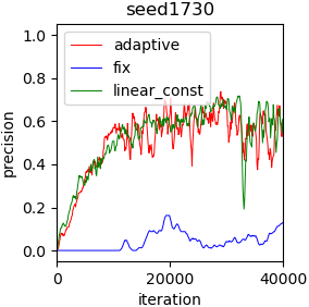
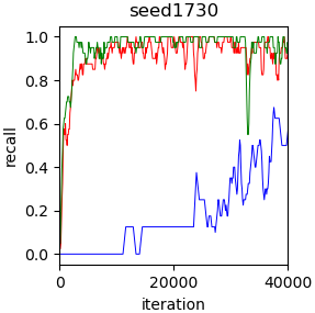
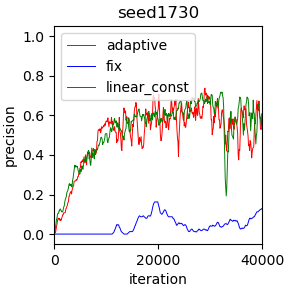
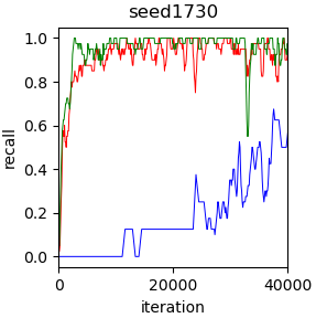
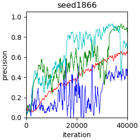
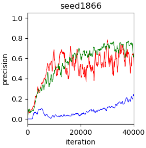
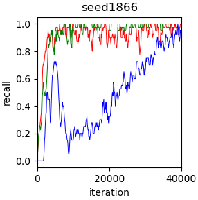
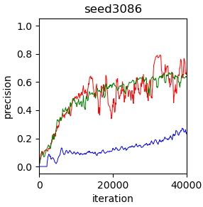
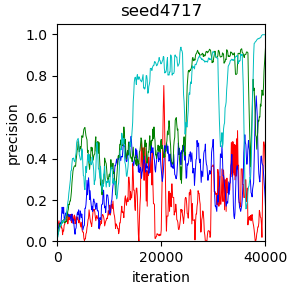
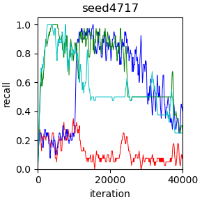
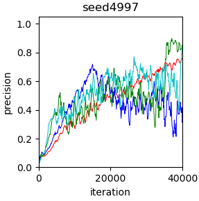
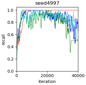
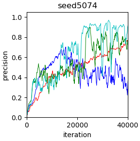
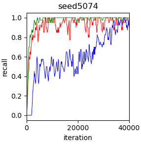
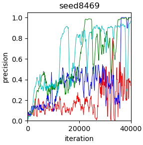
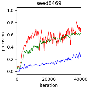
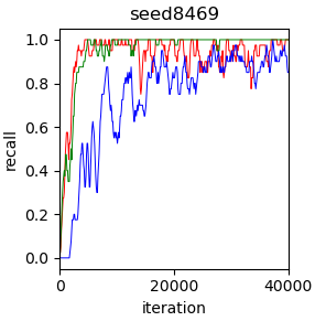
Panels (a) and (b) in Fig 3 show the precision and recall for each scaling strategy. Additional results with different seeds are reported in Section B. The “fix” strategy has low precision and does not learn well compared to the others. Both the “linear const” and “adaptive” strategies can roughly estimate distributions from an early stage and learn well. We see that learning with multiple scales is stable. The “adaptive” strategy is less dependent on the hyperparameters and can be used more universally (Wang et al.,, 2023).

3.3 Noise Injection and Data Scaling

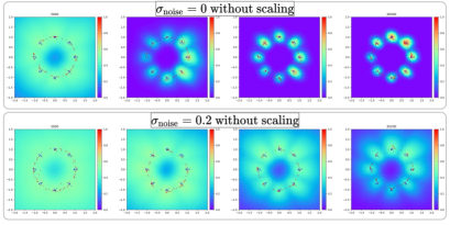
We numerically investigate the effectiveness of the noise injection and its relation to data scaling. At the beginning, let us consider the noise injection defined by $\tilde{{\bm{x}}}={\bm{x}}+\bm{\epsilon},\bm{\epsilon}\sim\mathcal{N}(\bm{0},\sigma_{\text{noise}}^{2}I)$. We compare the learning with $\sigma_{\text{noise}}=0$, i.e., the vanilla GAN, and the learning with positive $\sigma_{\text{noise}}$. Fig 4 (a) shows the training data $\{\tilde{{\bm{x}}}\}_{i=1}^{80}$, generated samples, and the discriminator’s outputs. As shown in the upper panels, the vanilla GAN learns faster, and the discriminator tends to have a large gradient. On the other hand, learning with noise injection yields a relatively smooth discriminator surface, meaning that mode collapse is mitigated. The precision and recall for each $\sigma_{\text{noise}}$ are shown in Fig B.2. We observe that the noise injection tends to stabilize the learning process compared to using the original training data. However, occasionally unstable behavior occurs even for noise injection.

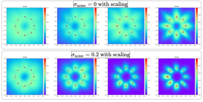
In Diffusion-GAN, both the data scaling and noise injection are incorporated, i.e., the training data $\boldsymbol{x}$ is transformed to $\tilde{{\bm{x}}}=s_{t}{\bm{x}}+\sqrt{1-s_{t}^{2}}\bm{\epsilon},\,\bm{\epsilon}\sim\mathcal{N}(\bm{0},\sigma_{\text{noise}}^{2}I)$. The scaling function $s_{t}$ is defined in the same way as that in Section 3.2, and the “adaptive” strategy is employed. Diffusion-GAN is compared with the vanilla GAN with the scaled generator $s_{t}G_{\theta}({{\bm{z}}})$ trained by the scaled data $\tilde{{\bm{x}}}=s_{t}{\bm{x}}$ without noise injection. The precision and recall for each $\sigma_{\text{noise}}$ are shown in Fig B.3. We see that overall the learning process is stable even in the case of $\sigma_{\mathrm{noise}}=0$, while Diffusion-GAN with $\sigma_{\mathrm{noise}}=0.05$ seems unstable. Fig 4 (b) shows the training data, generated samples, and the discriminator’s outputs. Unlike the results in Fig 4 (a), the noise does not have the effect of smoothing the surface of the discriminator’s outputs that much. This result suggests that scaling contributes significantly to stabilization and that the effect of noise injection is limited.

Refer to caption Refer to caption
(a) Learning without scaling (b) Learning with scaling
Figure 4: (a) Learning without scaling: the training data (red dots), generated data (blue dots), and the discriminator’s outputs (heatmap) are depicted. Upper panels: $\sigma_{\text{noise}}=0$. Lower panels: $\sigma_{\text{noise}}=0.2$. The number of training iterations ranges from 5000 to 20000 at every 5000 from right to left. (b) Learning with scaling: the training data (red dots), generated data (blue dots), and the discriminator’s outputs (heatmap) are depicted. Upper panels: “adaptive” scaling with $\sigma_{\text{noise}}=0$. Lower panels: Diffusion-GAN with “adaptive” scaling and $\sigma_{\text{noise}}=0.2$. The number of training iterations ranges from 10000 to 40000 at every 10000 from right to left.

4 Proposed Framework

Based on the analysis in Section 3, we propose a learning algorithm called Scale-GAN. We use the following notations. Let $\mu$ be the Lebesgue measure on the Borel algebra of a subset in the Euclidean space. Let us define $\|f\|_{1}=\int|f|\mathrm{d}{\mu}$ and $\|f\|_{\infty}=\sup_{{\bm{x}}}|f({\bm{x}})|$, which is regarded as the essential supremum according to the context. The function set ${\displaystyle L^{p}}(p=1,\infty)$ is defined as the set of all measurable functions for which $\|f\|_{p}<\infty$ holds. The expectation of the measurable function $f$ with respect to the probability density $p$ is denoted by $\mathbb{E}_{p}[f]$ or $\mathbb{E}_{{\bm{x}}\sim p}[f({\bm{x}})]$, meaning that $\int f({\bm{x}})p({\bm{x}})\mathrm{d}{\mu}({\bm{x}})$. The Lipschitz constant of $f$ is defined by $\|f\|_{\mathrm{Lip}}=\sup_{{\bm{x}}\neq{\bm{y}}}\frac{|f({\bm{x}})-f({\bm{y}})|}{\|{\bm{x}}-{\bm{y}}\|}$, where $\|\cdot\|$ is the Euclidean norm. For $\delta\in[0,1/2)$, let us define $\mathcal{U}_{\delta}=\{f\in L^{\infty}\,|\,\delta<\inf{f},\,\sup{f}<1-\delta\}$. Let $[a]_{+}=\max\{a,0\}$ for $a\in\mathbb{R}$.

4.1 Learning Algorithm

In Section 3, we find that data scaling contributes not only to counteracting overfitting but also to stabilization. Adding a diffusion term suggested that data augmentation updates the generator in a different direction than it should. Based on this idea, we consider data augmentation with scaling alone.

In addition to the data augmentation, let us consider the regularization. As discussed in Mangalam and Garg, (2021), the generator is prone to catastrophic forgetting and mode collapse when the discriminator’s outputs differ significantly among modes. Thus, stabilization of the discriminator is critical. We use the variance-based regularization $\mathbb{E}_{t}[\mathbb{V}_{p_{t}}[\widetilde{D}]|t]$ to the discriminator $\widetilde{D}(y,t)$, where $p_{t}$ is the distribution of the scaled data. A simple calculation leads that this regularization is an upper bound of the expectation of the approximate derivative, $\mathbb{E}_{t}[\mathbb{E}_{p_{t}(x)\otimes p_{t}(y)}[\frac{|\widetilde{D}(x,t)-\widetilde{D}(y,t)|}{\|x-y\|}]^{2}]$, up to a constant factor. Our variance regularization is similar to the NICE regularization (Ni and Koniusz,, 2024), which is an empirical approximation of $\mathbb{E}_{x\sim p_{0}}[\mathbb{V}_{s}[D(x\circ s)]|x],s\sim N_{d}({\bm{1}},\beta^{2}{\bm{I}})$, where $p_{0}$ is the data distribution. The paper’s author proved that the NICE regularization approximates the gradient penalty for the discriminator. Compared to some popular gradient-based regularization (Arjovsky et al.,, 2017; Gulrajani et al.,, 2017; Zhou et al.,, 2019), the variance-based regularization has an advantage for computation efficiency as well as NICE. In Section 4.2, we show that our variance regularization leads to the invariance of gradient direction under the data scaling. This is an important feature that mitigates the imbalance of the convergence speed between the discriminator and generator in the GAN learning process.

We introduce the loss function for Scale-GAN. The learning algorithm is obtained through an empirical approximation of the loss function. Let ${\bm{z}}$ be the latent variable of the generator having the distribution $p_{z}$. The distribution of the scaling intensity, $t$, is denoted by $\pi(t)$ on the interval $[0,T]$. Here, $T$ is a fixed positive value, while $T$ can be variable in practical learning algorithms. The proposed framework for Scale-GAN is given by the min-max optimization problem,

$\displaystyle\min_{G}\max_{\widetilde{D}}\mathbb{E}_{t\sim\pi}\big{[}L_{p_{0}}(G,\widetilde{D})-\lambda\mathbb{V}_{p_{0}}[\widetilde{D}(s_{t}{\bm{x}},t)]\big{]},$ (1)

with

$\displaystyle L_{p_{0}}(G,\widetilde{D}):=\mathbb{E}_{p_{0}}[\log\widetilde{D}(s_{t}{\bm{x}},t)]+\mathbb{E}_{{\bm{z}}}[\log(1-\widetilde{D}(s_{t}G({\bm{z}}),t))]$

for the data distribution $p_{0}({\bm{x}}),{\bm{x}}\in\mathcal{X}$. Here, $\lambda\geq 0$ is the regularization parameter. The learning algorithm with an empirical approximation of (1) is illustrated in Section D.1.

4.2 Theoretical Analysis

This section is devoted to revealing three theoretical properties of Scale-GAN; i) invariance property of the gradient direction for the generator’s learning, ii) the bias induced by the variance regularization and iii) relation between the estimation error bound and the scaling strategy. The property i) means that the data scaling will not degrade the efficiency of the generator learning. Due to ii), we can quantitatively understand the effect of the regularization. The result iii) provides a guideline on how to design the scaling $s_{t}$ to balance the learning stability and data-generation quality.

It is important to study the properties of the optimal discriminator for the inner maximization problem of (1). In the below, the discriminator on $\mathcal{X}$ (resp. $\mathcal{X}\times[0,T]$) is denoted by $D$ (resp. $\widetilde{D}$).

Theorem 1.

Suppose that $\mathcal{X}$ is $[0,1]^{d}$ or $\mathbb{R}^{d}$. Let $q({\bm{y}}),{\bm{y}}\in\mathcal{X}$ be the probability density of the generated sample ${\bm{y}}=G({\bm{z}}),{\bm{z}}\sim p_{z}$. Suppose $\|p_{0}\|_{\infty}<\infty$ and $\frac{p_{0}}{p_{0}+q}\in\mathcal{U}_{\delta}$ for a $\delta\in[0,1/2)$. Let $s_{t},t\in[0,T]$ be a strictly positive scaling function. Then, the following maximization problem has the unique optimal solution $\{\widetilde{D}(\cdot,t)\}_{t\in[0,T]}\subset\mathcal{U}_{0}$,

$\displaystyle\max_{\begin{subarray}{c}\widetilde{D}(\cdot,t)\in\mathcal{U}_{0},\\ 0\leq t\leq T\end{subarray}}\mathbb{E}_{t\sim\pi}[L_{p_{0}}(G,\widetilde{D})-\lambda\mathbb{V}_{p_{0}}[\widetilde{D}(s_{t}{\bm{x}},t)]$

Furthermore, the optimal discriminator satisfies $\widetilde{D}(s_{t}{\bm{x}},t)=\widetilde{D}({\bm{x}},0)$ for $({\bm{x}},t)\in\mathcal{X}\times[0,T]$.

The proof is deferred to Section D.2. In the vanilla GAN, the explicit expression of the optimal discriminator is obtained. In our case, however, such an explicit expression is unavailable due to the regularization term. In the proof, we use the fact that the objective function is concave in the discriminator. The concavity ensures that the Gâteaux differential (Kurdila and Zabarankin,, 2005) of the objective function leads the condition on the global optimality. Then, we obtain a cubic equation of $\widetilde{D}({\bm{x}},t)$ at each ${\bm{x}}$ and $t$. Analyzing the cubic equation, we can prove the existence of the optimal solution. The uniqueness comes from the strict concavity of the objective function.

Remark 1.

The assumption $\frac{p_{0}}{p_{0}+q}\in\mathcal{U}_{\delta}$ means that $q/p_{0}$ is bounded away from zero and infinity on $\mathcal{X}$.

4.2.1 Invariance of Gradient Direction

For a fixed generator $G_{\theta}$, suppose that the optimal discriminator $\widetilde{D}({\bm{y}},t)$ is obtained. Theorem 1 guarantees the equality $\widetilde{D}(s_{t}{\bm{x}},t)=\widetilde{D}({\bm{x}},0)$. Then, we have $\nabla_{{\bm{y}}}\widetilde{D}(s_{t}{\bm{x}},t)=\frac{1}{s_{t}}\nabla_{{\bm{y}}}\widetilde{D}({\bm{x}},0)$. At the optimal discriminator, the gradient vector of the objective function in (1) with respect to $\bm{\theta}$ is $\mathbb{E}_{{\bm{z}}}[\frac{\nabla_{\theta}G_{\theta}({\bm{z}})\nabla_{{\bm{y}}}\widetilde{D}(G_{\theta}({\bm{z}}),0)}{-1+\widetilde{D}(G_{\theta}({\bm{z}}),0)}]$, which is independent of the distribution of the scaling intensity $\pi(t)$. Since $s_{0}=1$, the above gradient is nothing but the gradient for the vanilla GAN. Note that the NICE regularization (Ni and Koniusz,, 2024) does not induce such an invariance property.

As illustrated in Section 3.1, the small scaling will make slower progress in learning the discriminator. In contrast, the learning of the generator is not affected by the scaling that much. On the other hand, if the noise is also injected, the generator’s gradient direction is disturbed. As a result, the convergence of the generator becomes slower. Hence, the scaling without noise is thought to improve the balance of the learning progress for the discriminator and generator compared to Diffusion-GAN, in which the convergence of both the discriminator and generator becomes slower due to the noise injection. The above discussion is confirmed by numerical experiments in Section 5.2.

4.2.2 Bias induced by Variance Regularization

For $\lambda=0$, the probability distribution corresponding to the optimal generator is $p_{0}$ (Goodfellow et al.,, 2014). Let us extend this to learning with regularization. Let $q_{\lambda}$ be the probability density corresponding to the optimal generator of (1). Under additional assumptions to Theorem 1, the upper bound of $\|p_{0}-q_{\lambda}\|_{\infty}$ is evaluated as follows. The detailed assumptions and the proof are found in Section D.3.

Theorem 2.

Let $\mathcal{X}$ be $[0,1]^{d}$ or $\mathbb{R}^{d}$. Suppose $\|p_{0}\|_{\infty}<\infty$ and $\|p_{0}\|_{\mathrm{Lip}}<\infty$. Let $q_{\lambda}$ be the probability density corresponding to the optimal generator of (1). Then, $\|p_{0}-q_{\lambda}\|_{\infty}=O(\lambda^{\frac{1}{d+3}})$ holds.

Theorem 2 suggests that the variance regularization is close to the regularization with $L_{\infty}$-norm on the set of probability densities.

4.2.3 Estimation Error Bound

We apply the statistical analysis of GAN introduced by Puchkin et al., (2024) and Belomestny et al., (2023). Let us assume $\mathcal{X}=[0,1]^{d}$. For i.i.d. training data ${\bm{x}}_{1},\ldots,{\bm{x}}_{n}\sim p_{0}$ and i.i.d. scaling intensity $t_{1},\ldots,t_{n}\sim\pi$, the empirical approximation of (1) is given by the min-max optimization problem,

$\displaystyle\min_{G\in\mathcal{G}}\max_{\widetilde{D}\in\widetilde{\mathcal{D}}}\ \frac{1}{n}\sum_{i}\log\widetilde{D}(s_{t_{i}}{\bm{x}}_{i},t_{i})+\frac{1}{n}\sum_{i}\log(1-\widetilde{D}(s_{t_{i}}G({\bm{z}}_{i}),t_{i}))-\lambda\widetilde{\mathbb{V}}[\widetilde{D}],$ (2)

where $\widetilde{\mathbb{V}}[\widetilde{D}]$ is an empirical approximation of the variance regularization. Deep neural networks (DNNs) are used for $\mathcal{\widetilde{D}}$ and $\mathcal{G}$. In our theoretical analysis, we consider DNNs with the rectified quadratic activation function (ReQU), which is defined by the square of ReLU. Learning using ReQU-based DNNs enables us to simultaneously approximate function value and the derivative, which is the preferable property for our purpose; see (Puchkin et al.,, 2024) for details.

The set of probability densities corresponding to $\mathcal{G}$ is denoted by $\mathcal{Q}$, i.e., the set of the push-forward probability density of $p_{z}$ by $G\in\mathcal{G}$. Let $\widehat{q}_{\lambda}\in\mathcal{Q}$ be the probability density of the trained generator. The estimation accuracy is evaluated by the JS divergence,

$\displaystyle\mathrm{JS}(p_{0},\widehat{q}_{\lambda})=\frac{1}{2}\mathbb{E}_{p_{0}}[\log\frac{2p_{0}}{p_{0}+\widehat{q}_{\lambda}}]+\frac{1}{2}\mathbb{E}_{\widehat{q}_{\lambda}}[\log\frac{2\widehat{q}_{\lambda}}{p_{0}+\widetilde{q}_{\lambda}}].$

As the function class of $p_{0}$ and $G_{0}$, let us consider the Hölder class of order $\beta$, i.e., $\mathcal{H}^{\beta}(\mathcal{X})$ endowed the norm $\|\cdot\|_{\mathcal{H}^{\beta}}$. Let us define

$\displaystyle\mathcal{H}^{\beta}(\mathcal{X},B)=\{f\in\mathcal{H}^{\beta}(\mathcal{X})|\|f\|_{\mathcal{H}^{\beta}}\leq B\},$
and $\displaystyle\ \mathcal{H}_{\Lambda}^{\beta}(\mathcal{X},B)=\{f\in\mathcal{H}^{\beta}(\mathcal{X},B)|\Lambda^{-2}I_{d\times d}\preceq\nabla_{x}f^{T}\nabla_{x}f\preceq\Lambda^{2}I_{d\times d}\}$

accordig to Puchkin et al., (2024). Note that $G_{0}\in\mathcal{H}^{1+\beta}_{\Lambda}(\mathcal{X})$ leads to $p_{0}\in\mathcal{H}^{\beta}(\mathcal{X})$. Without loss of generality, we assume that $\pi(t)$ is the uniform distribution on $[0,1]$ for the continuous scaling intensity. Suppose $\sup_{\widetilde{D}\in\widetilde{\mathcal{D}}}\|\widetilde{D}\|_{\mathrm{Lip}}\leq L$ for a constant $L>0$.

Theorem 3.

Suppose that the generator $G_{0}$ of the data distribution $p_{0}\in\mathcal{H}^{\beta}(\mathcal{X})$ satisfies $G_{0}\in\mathcal{H}_{\Lambda}^{1+\beta}([0,1]^{d},H_{0})$ for $\beta>2,H_{0}>0$ and $\Lambda>1$. For the scaling function $t\mapsto s_{t}$, suppose $1/s\in\mathcal{H}^{\alpha}([0,1])$ and $L\|s\|_{\mathcal{H}^{1}}\lesssim n^{c^{\prime}}$ for constants $\alpha>2$ and $c^{\prime}>0$. Then, there exist ReQU-based DNNs, $\mathcal{G}$ and $\widetilde{\mathcal{D}}$, such that the following holds with high probability greater than $1-\delta$,

$\displaystyle\mathrm{JS}(p_{0},\widehat{q}_{\lambda})$ $\displaystyle\lesssim\bigg{[}\max_{q\in\mathcal{Q}}\|\frac{p_{0}}{p_{0}+q}\|_{\mathcal{H}^{\beta}}-\frac{1}{8\sqrt{d}}\cdot\frac{L}{\|1/s\|_{\mathcal{H}^{\alpha}}}\bigg{]}_{+}^{2}+\bigg{\{}\bigg{(}\frac{L}{\|1/s\|_{\mathcal{H}^{\alpha}}}\bigg{)}^{2}+c\bigg{\}}\bigg{(}\frac{\log{n}}{n}\bigg{)}^{\frac{2\beta}{2\beta+d}}+\frac{\log(1/\delta)}{n}+\lambda.$ (3)

In the above, $c$ is a positive constant depending only on $d,\beta,\Lambda,c^{\prime}$ and $H_{0}$.

The proof is shown in Section D.4. Theorem 3 indicates that $s_{t}$ controls the bias(1st term)-variance(2nd term) trade-off in the estimation error bound. The order of the variance term coincides with the min-max optimal rate for the class of probability densities in $\mathcal{H}^{\beta}(\mathcal{X})$. In this case, however, the class of $p_{0}$ is slightly restricted by the push-forward with $G_{0}$. The estimation error for the vanilla GAN is recovered from $\lambda=0$ and $s_{t}=1$ (Puchkin et al.,, 2024). The scaling with a large $\|1/s\|_{\mathcal{H}^{\alpha}}$, such as $s_{t}=e^{-Mt}$ with $1\ll M\leq n^{c^{\prime}}/L$, leads to a small variance and a large bias. When $L$ is a large constant, and the first term of the upper bound vanishes, the data augmentation with scaling will improve the estimation accuracy.

4.2.4 Invertible Data Augmentation

Let us consider an extension of data scaling. A remarkable property of data scaling is that it is an invertible transformation. For invertible data augmentations (DAs), some properties similar to those of Scale-GAN hold, including the expression of the optimal discriminator in Theorem 1, the effect of variance regularization in Theorem 2, and the invariance of gradient direction shown in Section 4.2.1. Theorem 3 concerning estimation accuracy also holds with minor modifications.

The invertible data augmentation we consider here is formulated as follows. Let $S_{t}:\mathcal{X}\rightarrow\mathcal{X}$ be a transformation on $\mathcal{X}$ with the parameter $t\in{T}$ such that $S_{t}^{-1}(S_{t}({\bm{x}}))={\bm{x}}$ holds for ${\bm{x}}\in\mathcal{X}$ with inverse map $S_{t}^{-1}$. In what follows, parentheses for the transformation are omitted; that is, we use the notation $S_{t}{\bm{x}}$ or $S_{t}^{-1}{\bm{x}}$ for simplicity. In the learning process, the data scaling is replaced with the data transformation with $S_{t}$ meaning that the pair $(S_{t}{\bm{x}},t)$ is substituted into the discriminator in (2). Such a learning procedure is referred to as generalized Scale-GAN. Detailed analysis of the generalized Scale-GAN is presented in Section D.5.

The estimation accuracy of the generalized Scale-GAN is roughly given by

$\displaystyle\mathrm{JS}(p_{0},\widehat{q}_{\lambda})$ $\displaystyle\lesssim\bigg{[}\max_{q\in\mathcal{Q}}\|\frac{p_{0}}{p_{0}+q}\|_{\mathcal{H}^{\beta}}-\frac{1}{8\sqrt{d}}\cdot\frac{L}{\mathcal{J}_{\mathrm{DA}}}\bigg{]}_{+}^{2}+\bigg{\{}\bigg{(}\frac{L}{\mathcal{J}_{\mathrm{DA}}}\bigg{)}^{2}+c\bigg{\}}\bigg{(}\frac{\log{n}}{n}\bigg{)}^{\frac{2\beta}{2\beta+d}}$ (4)

with high probability, where $\mathcal{J}_{\mathrm{DA}}$ is the coefficient depending on the data augmentation employed the learing algorithm. For the invertible DA $S_{t},t\in{T}$, let us define $\phi_{S^{-1}}({\bm{x}},t)={S_{t}}^{-1}{\bm{x}}\in\mathcal{X}$. For the single DA, $\{S_{t}\,:\,t\in{T}\}$, suppose $\phi_{S^{-1}}\in\mathcal{H}^{\alpha}(\mathcal{X}\times{T}),\alpha>2$. Then, we have

$\displaystyle\mathcal{J}_{\mathrm{DA}}=\frac{1+\|\phi_{S^{-1}}\|_{\mathcal{H}^{\alpha}}}{2}.$

Furthermore, suppose that $B$ invertible data augmentations, $S_{i,t_{i}},t_{i}\in{T}_{i},i=1,\ldots,B$ such that $\phi_{S_{i}^{-1}}\in\mathcal{H}^{\alpha_{i}}(\mathcal{X}\times{T_{i}}),\alpha_{i}>2$, are used. In this case, the augmented data, $S_{i,t_{i}}{\bm{x}},\,i\in[B],t_{i}\in{T}_{i}$, is fed into the GAN algorithm, where the index $i$ and the parameter $t_{i}$ are randomly selected. Then, we have

$\displaystyle\mathcal{J}_{\mathrm{DA}}=\frac{\sqrt{B}+\max_{i\in[B]}\|\phi_{{S_{i}}^{-1}}\|_{\mathcal{H}^{\alpha_{i}}}}{2}.$
Example 1 (Scaling).

For the data-scaling, ${\bm{x}}\mapsto S_{t}{\bm{x}}=s_{t}{\bm{x}}$, the map $\phi_{S^{-1}}$ is defined by $\phi_{S^{-1}}({\bm{x}},t)={\bm{x}}/s_{t}$. Hence, the Hölder norm is $\|\phi_{S^{-1}}\|_{\mathcal{H}^{\alpha}}=\|1/s\|_{\mathcal{H}^{\alpha}}$, which leads to $\|1/s\|_{\mathcal{H}^{\alpha}}/2\leq\mathcal{J}_{\mathrm{DA}}=(1+\|1/s\|_{\mathcal{H}^{\alpha}})/2\leq\|1/s\|_{\mathcal{H}^{\alpha}}$.

Example 2 ($\pi/2$ rotation).

The $\pi/2$ rotation is realized by the permutation on pixels. Suppose the pixel of the image is indexed by $(i,j)$ such that $(i,j)\in\mathbb{Z}\times\mathbb{Z},|i|,|j|\leq v$. Then, $\pi/2$ rotation of the image maps $(x_{i,j})$ to $(x_{i,j}^{\prime})=(x_{-j,i})$, which is simply a permutation. Thus, the $\pi/2$ rotation is invertible. Similarly, $\pi$ and $3\pi/2$ rotations are also invertible transformations. The rotation with a fixed angle $\pi/2$ is represented by $S_{t}$ with the singleton $T=\{\pi/2\}$. Then, the Hölder norm of $\phi_{S^{-1}}$ is $\|\phi_{S^{-1}}\|_{\mathcal{H}^{\alpha}}=1$. When rotations with $0,\pi/2,\pi$, and $3\pi/2$ angles are used, we have $\mathcal{J}_{\mathrm{DA}}=(\sqrt{4}+1)/2=1.5$.

Example 3 (Saturation).

Each pixel of the RGB image, $(r,g,b)\in[-1,1]^{3}$, is mapped to $(r^{\prime},g^{\prime},b^{\prime})$ by the saturation transformation $(r,g,b,1)\mapsto(r^{\prime},g^{\prime},b^{\prime},\ast)=(tI_{4}+(1-t)\bm{v}\bm{v}^{T})(r,g,b,1)^{T}$, where $t$ is a positive parameter sampled from $\pi(t)$ and $\bm{v}\in\mathbb{R}^{4}$ is a fixed unit vector (Karras et al., 2020a, ). The log-normal distribution often applies as $\pi(t)$. Here, we assume $t$ is bounded below by a positive constant, i.e., $t\geq t_{\min}>0$. At each pixel, the inverse map is defined by the linear transformation with the matrix $t^{-1}I_{4}+(1-t^{-1})\bm{v}\bm{v}^{T}$. Then, the Hölder norm of $\phi_{S^{-1}}({\bm{x}},t)$ is of the order $\|\phi_{S^{-1}}\|_{\mathcal{H}^{\alpha}}=O((1/t_{\min})^{\alpha+1})$. The coefficient $\mathcal{J}_{\mathrm{DA}}$ is also $O((1/t_{\min})^{\alpha+1})$.

The data augmentation using only pixel blitting, such as the rotation, does not significantly impact on the estimation accuracy. On the other hand, the color formation such as data-scaling or saturation can greatly change the balance between the bias and the variance of the estimation error bound.

5 Numerical Experiments

We first investigate the effects of the variance regularization using the synthetic dataset in Section 3. The results are shown in Section C.1. Overall, the regularized Scale-GAN with an appropriate $\lambda$, such as $\lambda=0.1$ to $0.5$, outperforms non-regularized Scale-GAN with $\lambda=0$. However, the recall for the learning with strong regularization, such as $\lambda=5,10$, is degraded, meaning that the generator misses some modes.

Next, in Sections 5.1 and 5.2, we examine the effectiveness of the proposed method using some benchmark datasets. Based on the above result, the regularization parameter $\lambda$ is set to around $0.1$. Though the benchmark data is much larger than the above synthetic data, we show that the Scale-GAN with the regularization parameter in the above properly works.

5.1 Image Generation

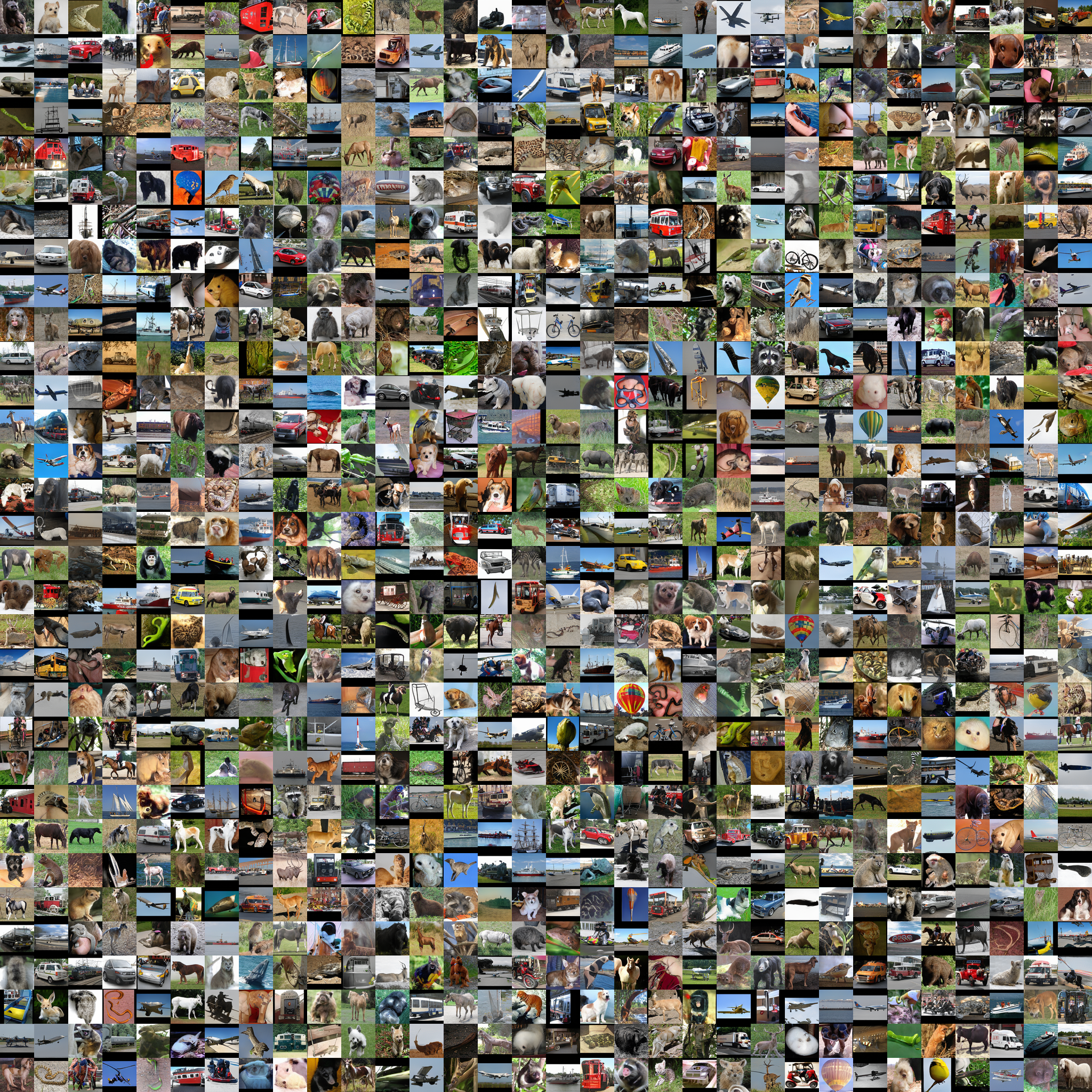
The effectiveness of the proposed method is confirmed in image generation, which is the standard task in GAN. The three datasets, CIFAR-10, STL-10, and LSUN-Bedroom are used. CIFAR-10 (Krizhevsky et al.,, 2009) consists of 50k images of the size $32\times 32\times 3$ in 10 classes. STL-10 (Coates et al.,, 2011) consists of 100k images of the size $64\times 64\times 3$ in 10 classes. While the original resolution of STL-10 is $96\times 96\times 3$, we resized it to compare with past studies. LSUN-Bedroom (Yu et al.,, 2016) includes 200k images of bedrooms of the size $256\times 256\times 3$. We assess the image quality in terms of sample fidelity (FID) and sample diversity (recall), which are used in Wang et al., (2023).

We compare our method with StyleGAN2 (Karras et al., 2020b, ), StyleGAN2+DiffAug (Zhao et al.,, 2020), StyleGAN2+ADA (Karras et al., 2020a, ), and Diffusion-GAN with StyleGAN2 (Karras et al., 2020b, ). Also we use StyleGAN2 in Scale-GAN.

Hyperparameters for existing methods are defined as the same as those in Wang et al., (2023). Also, our method uses almost the same hyperparameters, while some of them are adjusted based on preliminary experiments. The detailed hyperparameters are summarized in Section C.2. The distribution of the scaling intensity, $\pi_{0}$, on $\{1,\ldots,T\}$ has two choices, “uniform” and “priority”. The “uniform” distribution is defined by $\pi_{0}(t)=1/T$ used in Section 3.2. Note that the end point $T$ can change from iteration to iteration according to the scaling strategy. The “priority” distribution is defined by $\pi_{0}(t)\propto t$, which is recommended in Wang et al., (2023). Hence, the priority distribution is used in Diffusion-GAN. On the other hand, in our method, the uniform distribution is used for CIFAR-10 and STL-10, and the priority distribution is used for LSUN-Bedroom. The hyperparameter $d_{\mathrm{target}}$ in the adaptive strategy of $T$ is determined according to Wang et al., (2023). Furthermore, $T$ is clipped to the interval $[T_{\min},T_{\max}]$. The scaling function $s_{t}$ is determined by $\beta_{0}$ and $\beta_{T}$; see Section 3.2. In Diffusion-GAN, $\sigma_{\mathrm{noise}}=0.05$, $\beta_{0}=0.0001$ and $\beta_{T}=0.02$ are used. In our method, a larger $\beta_{T}$ properly works compared to Diffusion-GAN.

Table 1 shows the results of image generation on each benchmark dataset. The upper four methods are cited from the numerical results in Wang et al., (2023), and the lower two methods show the numerical results conducted using our computation environment. In terms of the FID score, our method outperforms the other methods by a clear margin. Also, the recall of our method attains higher values than the others.

The computational cost per iteration for Scale-GAN is approximately equivalent to that of Diffusion-GAN. For the same computation time, Scale-GAN outperforms Diffusion-GAN in data-generation quality. For instance, on the LUSN-Bedroom dataset, Scale-GAN achieves the optimal FID score for Diffusion-GAN in roughly one-fourth of the computational time.

Table 1: Image generation results on benchmark datasets: CIFAR-10, STL-10, and LSUN-Bedroom. We highlight the best and second best results in each column with bold and underline, respectively. Lower FIDs indicate better fidelity, while higher Recalls indicate better diversity.
CIFAR-10 STL-10 LSUN-Bedroom
(32 $\times$ 32) (64 $\times$ 64) (256 $\times$ 256)
Methods FID $\downarrow$ Recall $\uparrow$ FID $\downarrow$ Recall $\uparrow$ FID $\downarrow$ Recall $\uparrow$
StyleGAN2 8.32 0.41 11.70 0.44 3.98 0.32
StyleGAN2+DiffAug 5.79 0.42 12.97 0.39 4.25 0.19
StyleGAN2+ADA 2.92 0.49 13.72 0.36 7.89 0.05
Diffusion-GAN 3.19 0.58 11.43 0.45 3.65 0.32
Diffusion-GAN(our re-experiment) 3.39 0.57 11.53 0.45 3.53 0.25
Scale-GAN(proposal) 2.87 0.60 11.37 0.45 1.90 0.36

5.2 Additional Experiments on CIFAR-10

Gradient Direction.

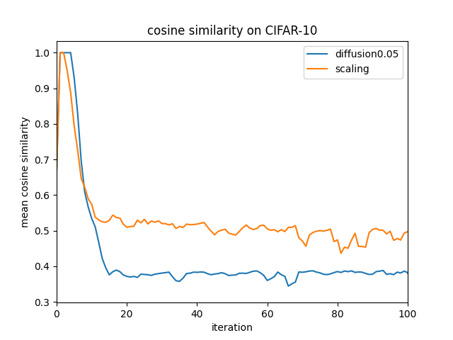
As shown in Section 4.2, if the optimal discriminator is obtained at each learning iteration, the gradient direction passed to the generator is independent of the scaling. This property holds when the expectation in the objective function is exactly calculated. In the beginning, let us compare the gradient direction of the proposed method with that of Diffusion-GAN in the empirical situation. The effect of data augmentation, ${\bm{x}}\mapsto\widetilde{{\bm{x}}}$, at the scaling intensity $t$ on the gradient direction is evaluated by the averaged cosine similarity between $\nabla{}\widetilde{D}(\widetilde{{\bm{x}}},t)$ and $\nabla{}\widetilde{D}({\bm{x}},0)$ for the distribution of $({\bm{x}},\widetilde{{\bm{x}}},t)$. Fig 5 shows the result on CIFAR-10. For Diffusion-GAN, the intensity of diffusion is set to $\sigma_{\mathrm{noise}}=0.05$. In both learning methods, $\pi_{0}$ is the uniform distribution on $\{1,\ldots,T\}$, and the adaptive strategy is used for the scaling. Overall, Scale-GAN provides a gradient closer to the gradient of the original data than Diffusion-GAN does. This indicates that the discriminator provides a gradient direction in which the generator’s learning will likely progress even under data augmentation. Therefore, Scale-GAN is expected to mitigate the imbalance of the convergence speed between the discriminator and generator more efficiently than Diffusion-GAN.

Setting: Effect of Each Component.

Table 2 shows the result of numerical experiments for some modified learning methods; i) StyleGAN2 with noise injection by $\widetilde{{\bm{x}}}={\bm{x}}+\sqrt{1-s_{t}^{2}}\sigma_{\mathrm{noise}}\bm{\epsilon}$, ii) Diffusion-GAN with $\beta_{T}=0.028$ that is larger than $\beta_{T}$ used in Table 1, iii) Diffusion-GAN with the variance regularization ($\beta_{T}=0.02,\lambda=0.1$), iv) Scale-GAN with a modified variance regularization ($\beta_{T}=0.028,\lambda=0.1$), and v) Scale-GAN without variance-based regularization ($\beta_{T}=0.028,\lambda=0$). The modified variance regularization is the regularization using second order moment with a fixed mean, $\lambda\mathbb{E}[(\widetilde{D}-1/2)^{2}]$. In the vanilla GAN, the optimal solution of the discriminator is the constant function $1/2$ when the generator is correctly specified. This fact motivates the usage of the modified variance regularization. Even using the modified variance regularization, the same theoretical properties in Section 4.2 hold for Scale-GAN. Examined methods i), ii), and iii), include noise injection.

Noise Injection and Data Scaling.

For StyleGAN2, the noise injection efficiently works. Indeed, the usefulness of the noise injection has been intensively studied in Feng et al., (2021) and other works. However, its performance is not as high as Diffusion-GAN and Scale-GAN. Diffusion-GAN with a stronger scaling yields no improvement in accuracy.

Regularization.

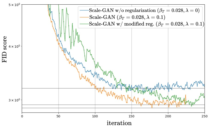
When Diffusion-GAN with the variance regularization and the original Diffusion-GAN are compared, the regularization does not improve the accuracy as much as Scale-GAN. As shown in v) of Table 2, Scale-GAN without regularization efficiently works compared to the existing methods. Furthermore, we see that the effect of the regularization on the FID score is significant when Scale-GAN w/o Var-reg and Scale-GAN are compared.

Modified Regularization.

The modified regularization’s effect is expected to be similar to the variance regularization in Scale-GAN. Table 2 shows that the accuracy of Scale-GAN with modified Var-reg is close to that of Scale-GAN. However, the modified regularization requires a longer training time to achieve high accuracy; see Section C.3. The slow learning is thought to be due to the effect of forcing the discriminator’s output to be close to $1/2$. This fact especially affects the learning behavior when the adaptive strategy is employed for data scaling. In this case, $r_{d}$ tends to become smaller even in overfitting, and $T$, which determines the scaling magnitude, does not become larger. As a result, the modified regularization does not sufficiently address the overfitting in the middle stage of learning, which is interpreted as a lack of good gradients and progress in learning.

Refer to caption
Figure 5: Averaged cosine similarity between $\nabla{D}(\widetilde{{\bm{x}}},t)$ and $\nabla{D}({\bm{x}},0)$ at each iteration on CIFAR-10. Blue solid line is Diffusion-GAN with $\sigma_{\mathrm{noise}}=0.05$, and orange solid line is Scale-GAN.
Table 2: Image generation results on CIFAR-10 for various learning methods. The FID and recall values for StyleGAN2 and Diffusion-GAN in the lower part are identical to those in Table 1, as cited from the numerical results in Wang et al., (2023). The result for Scale-GAN from Table 1 is also included. “Var-reg” denotes variance regularization, while “modified Var-reg” refers to its modified version.
Methods FID $\downarrow$ Recall $\uparrow$
i) StyleGAN2 w/ noise injection 3.87 0.56
ii) Diffusion-GAN: $\beta_{T}=0.028$ 3.39 0.57
iii) Diffusion-GAN w/ Var-reg. 3.18 0.57
iv) Scale-GAN w/ modified Var-reg. 2.89 0.57
v) Scale-GAN w/o Var-reg. 3.11 0.59
StyleGAN2 8.32 0.41
Diffusion-GAN:$\beta_{T}=0.02$ 3.19 0.58
Scale-GAN 2.87 0.60

6 Conclusions

This paper demonstrates, both theoretically and experimentally, that data scaling enhances learning stability in generative models. We show that data scaling regulates the bias-variance trade-off, improving estimation accuracy. Our findings offer valuable insights for designing effective scaling strategies to train generative models.

Appendix A Related Works

While GAN can generate high-quality images, learning instability and mode collapse have long been problems. Numerous methods have been proposed to solve these problems.

A.1 Loss functions, Regularization and Data Augmentation for GANs

Modifying loss functions is a possible approach to overcoming the instability problems. The loss function of the vanilla GAN (Goodfellow et al.,, 2014) is the Jensen-Shannon (JS) divergence, which often fails to learn a generator if the training data and generated data are easily separated. Toward the remedy of the instability issue, discrepancy measures such as Wasserstein distance (Arjovsky et al.,, 2017), squared loss (Mao et al.,, 2017), hinge loss (Miyato et al.,, 2018; Brock et al.,, 2018; Zhang et al.,, 2019) and maximum mean discrepancy (Li et al.,, 2017) have been studied and shown to contribute to stabilization. As shown in Wasserstein-GAN (Arjovsky et al.,, 2017), Lipschitz continuity of the discriminator plays a central role in stabilizing the learning process. By adding a penalty constraining the gradient of the discriminator to the objective function, Lipschitz continuity is prone to be satisfied (Gulrajani et al.,, 2017; Kodali et al.,, 2017; Adler and Lunz,, 2018; Petzka et al.,, 2018; Xu,, 2021; Mescheder et al.,, 2018; Zhou et al.,, 2019; Thanh-Tung et al.,, 2018). In addition, Miyato et al., (2018) proposed spectral normalization, which guarantees Lipschitz continuity by constraining the spectral norm of the weights. As an other approach, Adaptive Instance Normalization (Huang and Belongie,, 2017), proposed in the context of style transformation, is used in styleGAN (Karras et al.,, 2019) and attracted much attention for its significant contribution to improving image generation performance. The instability of GANs in the early stages of learning is considered to be partly due to the lack of overlap between the support of the generated samples and that of the training data. To address the problem, Roth et al., (2017) proposed a method for extending the support of the distribution by adding noise. Noise injection as a data augmentation is expected to bring support closer together and suppress the overfitting of the discriminator. However, suitable noise distribution heavily depends on the data domain, and thus, the noise injection is hard to implement in practice, as pointed out by Arjovsky and Bottou, (2017).

A.2 Fusion of GAN and Diffusion Models

In recent years, the diffusion model has also attracted considerable attention as a model that generates natural high-resolution images (Ho et al.,, 2020; Song and Ermon,, 2019). The diffusion model approximates the inverse process of the diffusion process, in which noise is added to the data, with a neural network, and generates data by repeated denoising. Since the learning of the diffusion model is formulated as the minimization problem of the loss function, such as the denoising score matching loss (Song and Ermon,, 2019), it can be trained more stably than GANs, which makes it easier to apply to large data sets. However, in the sampling phase, hundreds to thousands of DNN’s feedforward passes are required for a single image. Recent developments have enabled us to reduce the number of DNN’s computations to about ten iterations by using distillation (Salimans and Ho,, 2021) and higher-order differential equation approximation methods (Lu et al.,, 2022; Zheng et al.,, 2023). On the other hand, GANs usually need only one feed-forward pass for data generation. To combine the advantages of GANs and diffusion models, some frameworks have been recently developed. The Diffusion-GAN (Wang et al.,, 2023), inspired by the diffusion model, injects noise similar to the DDPM (Ho et al.,, 2020) into GAN’s training process to achieve stable computation and high-quality image generation. Xiao et al., (2021) proposed Denoising Diffusion GAN that uses GAN’s discriminator in the diffusion model to achieve both high accuracy and fast sampling. Besides the diffusion-GAN, the fusion of GANs and diffusion models have been considered by Zheng et al., (2022); Yin et al., 2024b ; Sauer et al., (2023); Kim et al., (2023); Yin et al., 2024a to improve the efficiency, speed, and quality of generative models, mainly focusing on diffusion models and distillation techniques to reduce computational costs. and distillation techniques to reduce computational costs.

Appendix B Additional Numerical Studies to Section 3

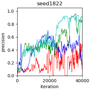
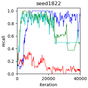
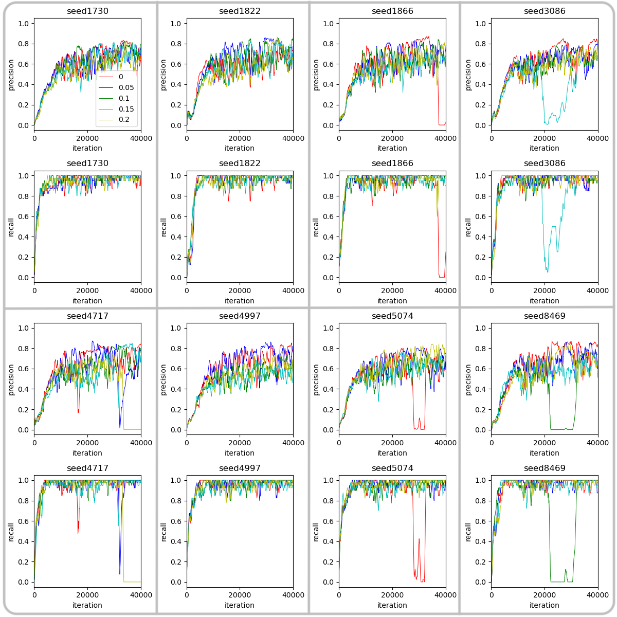
Numerical experiments in Section 3 are conducted with more seeds. The results are shown in Fig B.1. Each row corresponds to each seed. The panels (a), (b), and (c) show the results for four types of data scaling, and panels (d) and (e) show the results for three scaling strategies.

For the scaling, $s=0.25,0.5,1,1.5$, the discriminator $D_{\phi}$ and the scaled generator $sG_{\theta}$ are trained by the original GAN (Goodfellow et al.,, 2014) using $\{{\bm{y}}_{i}\}_{i=1}^{80},\,{\bm{y}}_{i}=s{\bm{x}}_{i}$ as true data. In Fig B.1, the panels (a) and (b) show precision and recall at each scaling for different seeds. The learning with $s=0.25$ shows that if the distribution is well covered (high recall) in the early stages of learning, the precision gradually increases, and the learning is successful. However, it has not escaped from the initial learning failure. These results can be explained by the size of the gradient, as shown in Fig B.1 (c). The gradient’s norm for $s=0.25$ is smaller than the other cases. The result indicates that abrupt changes in the discriminator are considered difficult to occur. Hence, the learning result will be significantly affected by the early stages of the learning process. On the other hand, for $s=1,1.5$, high recall is achieved in the early stages of learning. However, it is observed that the recall drops significantly from the middle to the latter half of the learning period, causing mode collapse. Also as shown in Fig B.1 (c), instability is manifested as mode collapse due to large gradients after the middle of the training phase.

Panels (d) and (e) in Fig B.1 show the precision and recall for each scaling strategy. The “fix” strategy has low precision and does not learn well compared to the others. Both the “linear const” and “adaptive” strategies can estimate rough distributions from an early stage and learn well. It is found that learning data at multiple scales simultaneously is stable. The “adaptive” strategy is preferable since it is less dependent on the hyperparameters and can be used more universally (Wang et al.,, 2023).

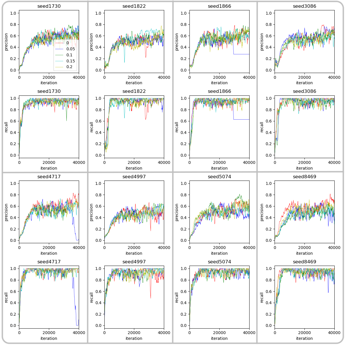
Fig B.2 shows supplementary numerical results in Section 3.3. We consider the noise injection, $\tilde{{\bm{x}}}={\bm{x}}+\bm{\epsilon},\bm{\epsilon}\sim\mathcal{N}(\bm{0},\sigma_{\text{noise}}^{2}I)$ for $\sigma_{\mathrm{noise}}\in\{0,0.05,0.1,0.15,0.2\}$. Numerical experiments conducted with several seeds are depicted. Each gray box corresponding to each seed includes two panels, the precision and recall to the learning iteration. The noise of any magnitude examined in the experiment can cause instability and may not contribute significantly to stabilization.

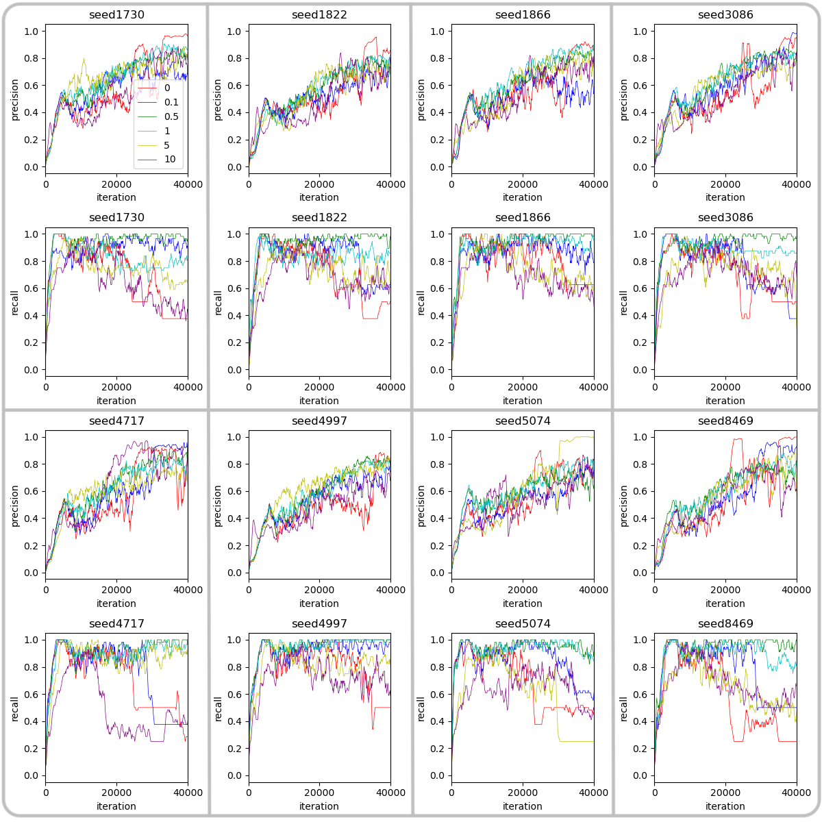
In the diffusion-GAN, both the data scaling and noise injection are incorporated, i.e., the training data $\boldsymbol{x}$ is transformed to $\tilde{{\bm{x}}}=s_{t}{\bm{x}}+\sqrt{1-s_{t}^{2}}\bm{\epsilon},\,\bm{\epsilon}\sim\mathcal{N}(\bm{0},\sigma_{\text{noise}}^{2}I)$. The scaling function $s_{t}$ is defined in the same way as those in Section 3.2, and the “adaptive” strategy is employed. The diffusion-GAN is compared with the GAN with the scaled generator $s_{t}G_{\theta}({{\bm{z}}})$ trained by the scaled data $\tilde{{\bm{x}}}=s_{t}{\bm{x}}$ without diffusion. Fig B.3 shows the precision and recall for the learning with several $\sigma_{\text{noise}}$. Each gray box includes two panels, the precision, and recall to the learning iteration, for each seed when the noise level $\sigma_{\mathrm{noise}}$ varies $0,0.05,0.1,0.15$, and $0.2$. We see that overall the learning process is stable, while the diffusion-GAN with $\sigma_{\mathrm{sigma}}=0.05$ seems unstable. The results in Fig B.3 suggests that scaling contributes significantly to stabilization and that the effect of noise imposition is limited.

Refer to caption Refer to caption Refer to caption Refer to caption Refer to caption
(a) data scaling:   (a) precision (b) data scaling:   (b) recall (c) data scaling:   (c) norm of gradient (d) scaling strategy:   (d) precision (e) scaling strategy:   (e) recall
Figure B.1: (a) precision for each scale, (b) recall for each scale, (c) averaged norm of discriminator’s gradient, (d) precision for each scaling strategy, and (e) recall for each scaling strategy are depicted. Each row corresponds to each seed. The scale $s$ is set to $0.25,0.5,1,$ and $1.5$ for (a), (b), and (c). As a scaling strategy, “fix”, “linear const”, or “adaptive” is used in (d) and (e).
Refer to caption
Figure B.2: Each gray box corresponds to each seed. Precision and recall for the learning with noise injection, $\widetilde{{\bm{x}}}={\bm{x}}+\sigma_{\mathrm{noise}}\bm{\epsilon},\bm{\epsilon}\sim\mathcal{N}(\bm{0},\sigma_{\text{noise}}^{2}I)$, are depicted at each learning iteration. The noise level $\sigma_{\mathrm{noise}}$ is set to $0,0.05,0.1,0.15$, and $0.2$.
Refer to caption
Figure B.3: Each gray box corresponds to each seed. Precision and recall for the learning with data scaling and noise injection, $\widetilde{{\bm{x}}}=s_{t}{\bm{x}}+\sqrt{1-s_{t}^{2}}\sigma_{\mathrm{noise}}\bm{\epsilon},\bm{\epsilon}\sim\mathcal{N}(\bm{0},\sigma_{\text{noise}}^{2}I)$ are depicted at each learning iteration The noise level $\sigma_{\mathrm{noise}}$ is set to $0,0.05,0.1,0.15$, and $0.2$. The scaling function $s_{t}$ is determined by the uniform distribution with adaptive strategy.

Appendix C Additional Numerical Studies to Section 5

All experiments in this paper are conducted on one or two of the following GPUs: NVIDIA RTX A5000(24GB memory), RTX A6000(48GB memory), and Tesla V100S(32GB memory). When two GPUs are used in parallel, the same type of GPU is used. The training time is almost the same as Diffusion-GAN, as the computational cost of the scale-wise variance regularization has little impact. As for the libraries, the environment was built according to Diffusion-GAN’s environment.yml.

C.1 Stability of Scale-wise Variance Regularization

We investigate the effects of scale-wise variance regularization using the same synthetic dataset as in Section 3. Fig C.1 shows the precision and recall when the scale-wise variance regularization is used for Scale-GAN. We observe that overall the regularized Scale-GAN with a positive $\lambda$ outperforms non-regularized Scale-GAN, i.e., $\lambda=0$ when the regularization parameter is appropriately determined, such as $\lambda=0.1$ or $0.5$. However, too strong regularization like $\lambda=5,10$ leads to instability. Indeed, the recall for the learning with $\lambda=5,10$ is degraded, meaning that the generator misses some modes.

Refer to caption
Figure C.1: Each gray box corresponds to each seed. Precision and recall for Scale-GAN with several regularization parameters are depicted at each learning iteration. The regularization parameter $\lambda$ is set to $0,0.1,0.5,1,5$, and $10$. The scaling function $s_{t}$ is determined by the uniform distribution with adaptive strategy.

C.2 Hyperparameters in Section 5.1

Some hyper-parameters in Diffusion-GAN are defined as follows.

  • $T$: The number of scales, $s_{1},\ldots,s_{T}$, used in the learning process of Diffusion-GAN.

  • $T_{\max},T_{\min}$: In Diffusion-GAN, $T$ can vary during the learning process, and its range is from $T_{\min}$ to $T_{\max}$ to which are predefined constants.

  • $I$: For the strategy of ”linear const”, $T$ at $i$-th step is determined by $\\ min\{i\ast 2T_{\max}/I,T_{\max}\}$. The parameter $I$ controls the increasing speed of $T$.

  • $r_{d}$: An estimate of how much the discriminator overfits the data.

  • $d_{\mathrm{target}}$: The threshold to determine when the parameter $T$ increases in the ”adaptive” strategy.

Hyperparameters used in Diffusion-GAN and Scale-GAN are summarized in the following.

  • Diffusion-GAN: for all three datasets, the following parameters are used:

    • priority distribution $\pi_{0}$ with adaptive strategy

    • $\beta_{0}=0.0001,\beta_{T}=0.02,T_{\min}=5,T_{\max}=1000,\sigma_{\mathrm{noise}}=0.05$.

  • Scale-GAN(proposed)

    • CIFAR-10:

      • *

        uniform distribution $\pi_{0}$ with adaptive strategy

      • *

        $\beta_{0}=0.0001,\beta_{T}=0.028,T_{\min}=5,T_{\max}=1000,\lambda=0.1$.

    • STL-10

      • *

        uniform distribution $\pi_{0}$ with adaptive strategy

      • *

        $\beta_{0}=0.0001,\beta_{T}=0.03,T_{\min}=5,T_{\max}=1500,\lambda=0.05$.

    • LSUN-Bedroom

      • *

        priority distribution $\pi_{0}$ with adaptive strategy

      • *

        $\beta_{0}=0.0001,\beta_{T}=0.028,T_{\min}=5,T_{\max}=1000,\lambda=0.1$.

In Diffusion-GAN, the parameters are the same as those in (Wang et al.,, 2023). The parameter $d_{\mathrm{target}}$ in the adaptive strategy is set to $0.6$.

The STL-10 dataset is known as a dataset with high variance, which is thought to be a reason that the larger scaling $\beta_{T}=0.03,T_{\text{max}}=1500$ works effectively.

Fig. C.2, and C.3 shows the generated sample images by Scale-GAN.

Refer to caption
Figure C.2: Generated sample images by Scale-GAN trained using CIFAR-10.
Refer to caption
Figure C.3: Generated sample images by Scale-GAN trained using STL-10.

C.3 Scale-GAN with Modified Regularization on CIFAR-10

Let us investigate the effect of several regularization terms for Scale-GAN. The uniform distribution $\pi_{0}$ with the adaptive strategy is employed to determine the scaling function $s_{t}$.

We compare Scale-GAN with scale-wise variance regularization ($\beta_{T}=0.02,\lambda=0.1$), i.e., the proposed method, Scale-GAN without regularization ($\beta_{T}=0.02,\lambda=0$), and Scale-GAN with modified regularization ($\beta_{T}=0.02,\lambda=0.1$). The scale-wise variance regularization is defined by the empirical approximation of $\lambda\mathbb{V}[D(\widetilde{{\bm{x}}},t)]$ for the joint distribution of the augmented data $\widetilde{{\bm{x}}}$ and the scale intensity $t$. On the other hand, the modified regularization is defined by the empirical approximation of $\lambda\mathbb{E}[(D(\widetilde{{\bm{x}}},t)-1/2)^{2}]$.

Fig C.4 shows the FID score at each learning iteration. The result indicates that the regularization efficiently attains a good FID score after a sufficient iteration. However, the convergence speed of Scale-GAN with modified regularization is slower than Scale-GAN with scale-wise variance regularization. Modified regularization is thought to make the adaptive strategy inefficient. More precisely, the expectation in $r_{d}=\mathbb{E}[\operatorname{sign}(\widetilde{D}({\bm{y}},t)-0.5)]$ for the adaptive strategy

$\displaystyle T\leftarrow T+\operatorname{sign}(r_{d}-d_{\text{target }})$ (C.1)

tends to be small, and the parameter $T$ does not take a large number, resulting in the scale intensity $t$ taking a small number.

Refer to caption
Figure C.4: FID scores for Scale-GAN w/o regularization, Scale-GAN, and Scale-GAN with modified regularization are depicted at each iteration for CIFAR-10 dataset.

Appendix D Supplementary of Proposed Framework

For theoretical analysis, let us prepare the following notations. For $0\leq\delta<1/2$, let us define $\lambda_{\delta}=\delta^{3}/10$, and

$\displaystyle\mathcal{U}_{\delta}$ $\displaystyle=\{f\in L^{\infty}\,|\,\delta<\inf f,\sup{f}<1-\delta\},$
$\displaystyle\Lambda_{\delta}$ $\displaystyle=[0,\lambda_{\delta}]\subset\mathbb{R},$
$\displaystyle\mathcal{Q}_{\delta,C}$ $\displaystyle=\left\{q\in L^{1}\cap L^{\infty}\,\bigg{|}\,\frac{p_{0}}{p_{0}+q}\in\mathcal{U}_{\delta},\,\|q\|_{\mathrm{Lip}}\leq C,\,\int q\mathrm{d}{\mu}=1\right\},$
$\displaystyle\mathcal{D}_{\delta}$ $\displaystyle=\left\{D\in L^{\infty}\,\big{|}\,\delta-5\lambda_{\delta}\bigg{(}\frac{1-\delta}{\delta}\bigg{)}^{2}<D<1-\delta+5\lambda_{\delta}\bigg{(}\frac{1-\delta}{\delta}\bigg{)}^{2}\right\}.$

For the probability density $p_{0}({\bm{x}})$, the function $q$ in $\mathcal{Q}_{\delta,C}$ should be non-negative, and thus $q$ is a probability density. When $p_{0}\in L^{\infty}$ and $\|p_{0}\|_{\mathrm{Lip}}\leq C$, we have $p_{0}\in\mathcal{Q}_{\delta,C}$. By the definition of $\lambda_{\delta}$, we see that $0<D<1$ holds for $D\in\mathcal{D}_{\delta},0\leq\delta<1/2$. Throughout the paper, all probability densities are strictly positive on their domain.

D.1 Learning Algorithm: Scale-GAN

The learning algorithm of Scale-GAN is similar to Diffusion-GAN (Wang et al.,, 2023). The main difference is the data augmentation. In Scale-GAN, only the data scaling is employed, while Diffusion-GAN used the noise injection in addition to data scaling. For i.i.d. training data ${\bm{x}}_{1},\ldots,{\bm{x}}_{n}\sim p_{0}$ and i.i.d. scales $t_{1},\ldots,t_{n}\sim\pi$, the empirical approximation of (1) is given by the min-max optimization problem,

$\displaystyle\min_{G\in\mathcal{G}}\max_{\widetilde{D}\in\widetilde{\mathcal{D}}}\frac{1}{n}\sum_{i}\log\widetilde{D}(s_{t_{i}}{\bm{x}}_{i},t_{i})+\frac{1}{n}\sum_{i}\log(1-\widetilde{D}(s_{t_{i}}G({\bm{z}}_{i}),t_{i}))-\lambda\widetilde{\mathbb{V}}[\widetilde{D}],$ (D.1)

where

$\displaystyle\widetilde{\mathbb{V}}[\widetilde{D}]=\frac{1}{n}\sum_{j=1}^{n}\left\{\frac{1}{n}\sum_{i}(\widetilde{D}(s_{t_{j}}{\bm{x}}_{i},t_{j})-\frac{1}{n}\sum_{i^{\prime}}\widetilde{D}(s_{t_{j}}{\bm{x}}_{i^{\prime}},t_{j}))^{2}\right\}$

is an empirical approximation of $\mathbb{E}_{\pi}[\mathbb{V}_{p_{0}}[\widetilde{D}]]$. The pseudo code of Scale-GAN is shown in Algorithm 1.

Algorithm 1 : Scale-GAN
Initialization: DNNs $G_{u},D_{\theta}$, distribution of latent variable $p_{z}$, scaling function $s_{t}$ and
                     intensity distribution $\pi(t)$ with hyper-parameters $\beta_{0},\beta_{T},T_{\min},T_{\max},d_{\text{target}}$, etc.
while $i\leq$ number of training iterations do
     $\#$Step I: Update Discriminator
  • Sample minibatch of $m$ noise samples ${\bm{z}}_{1},\ldots,{\bm{z}}_{m}\sim_{i.i.d.}p_{z}$.

  • Obtain generated sample ${\bm{y}}_{i}=G_{u}({\bm{z}}_{i}),\,i=1,\ldots,m$.

  • Sample minibatch of $m$ data ${\bm{x}}_{1},\ldots,{\bm{x}}_{m}$.

  • Sample scale intensity $t_{1},\ldots,t_{m}\sim\pi$.

  • Update discriminator $D_{\theta}$ by maximizing the objective function of (D.1) for the fixed $G_{u}$.

     $\#$Step II: Update Generator
  • Sample minibatch of $m$ noise samples ${\bm{z}}_{1},\ldots,{\bm{z}}_{m}\sim_{i.i.d.}p_{z}$.

  • Obtain generated sample ${\bm{y}}_{i}=G_{u}({\bm{z}}_{i}),\,i=1,\ldots,m$.

  • Sample scale intensity $t_{1},\ldots,t_{m}\sim\pi$.

  • Update discriminator by minimizing the objective function of (D.1) for the fixed $D_{\theta}$.

     $\#$Step III: Update scaling strategy
     if  $i\mod 4==0$ then
          Update $T$ by (C.1).
          Update the distribution of the scale intensity $\pi(t)$ using updated $T$.
     end if
end while

D.2 Proof of Theorem 1

Problem Setting

For the probability density $q$ on $\mathcal{X}$ and the discriminator $D:\mathcal{X}\rightarrow(0,1)$, let us define the regularized loss by

$\displaystyle F_{p_{0}}(q,D;\lambda):=L_{p_{0}}(q,D)-\lambda\mathbb{V}_{p_{0}}[D],\ \ L_{p_{0}}(q,D):=\mathbb{E}_{p_{0}}[\log D]+\mathbb{E}_{q}[\log(1-D)].$

For the probability density $p_{0}({\bm{x}}),\,{\bm{x}}\in\mathcal{X}$, let $p_{t}({\bm{y}})$ be the probability density of the scaled variable ${\bm{y}}=s_{t}{\bm{x}}$ on $s_{t}\mathcal{X}=\{s_{t}{\bm{x}}\,|\,{\bm{x}}\in\mathcal{X}\}$, where $s_{t}\in(0,1]$ is the scaling function with $s_{0}=1$. More concretely, $p_{t}({\bm{y}})=p_{0}({\bm{y}}/s_{t})/s_{t}^{d}$ holds. Likewise, for the probability density $q$ of the generator, the probability density $q_{t}$ is defined by $q_{t}({\bm{y}})=q({\bm{y}}/s_{t})/s_{t}^{d}$. Note that $q_{0}=q$ holds. Using a pre-specified probability density $\pi(t)>0$ for $t\in[0,T]$, Scale-GAN with the variance regularization is formulated as the min-max problem,

$\displaystyle\min_{\{q_{t}\}_{t\in[0,T]}}\max_{\{D_{t}\}_{t\in[0,T]}}\mathbb{E}_{t\sim\pi}\big{[}L_{p_{t}}(q_{t},D_{t})-\lambda\mathbb{V}_{p_{t}}[D_{t}]\big{]},$ (D.2)

for $D_{t}(\cdot)=\widetilde{D}(\cdot,t)$. The objective function of (D.2) is expressed as $\mathbb{E}_{t\sim\pi}[F_{p_{t}}(q_{t},D_{t};\lambda)]$.

Theoretical Analysis of Optimal Discriminator

We consider the optimal solution of (D.2) under the condition $\|p_{0}\|_{\infty}<\infty,q\in\mathcal{Q}_{\delta,\infty}$ and $D\in\mathcal{U}_{0}$. Note that the assumption $\frac{p_{0}}{p_{0}+q}\in\mathcal{U}_{\delta}$ ensures $\frac{p_{t}}{p_{t}+q_{t}}\in\mathcal{U}_{\delta}$ for $t\geq 0$. Under the assumption, $p_{0}$ and $q$ are positive almost everywhere with respect to $\mu$. Note that the set $\mathcal{U}_{\delta}$ is convex for $0\leq\delta<1/2$.

We confirm the strict concavity of the functional $D\mapsto F_{p_{0}}(q,D;\lambda)$ for $D\in\mathcal{U}_{0}$. The concavity of the functional $D\rightarrow L_{p_{0}}(q,D)$ and the convexity of the variance $D\mapsto\mathbb{V}_{p_{0}}[D]$ are clear. For $D_{1},D_{2}\in\mathcal{U}_{0}$ such that $\mu(D_{1}\neq D_{2})>0$, the set

$\displaystyle\{{\bm{x}}\in\mathcal{X}\,|\,\log(\alpha D_{1}({\bm{x}})+(1-\alpha)D_{2}({\bm{x}}))>\alpha\log D_{1}({\bm{x}})+(1-\alpha)\log D_{2}({\bm{x}})\}$

has a positive measure for $0<\alpha<1$. The same property holds for the function $D\mapsto\log(1-D)$. Therefore, the strict concavity of $D\mapsto F_{p_{0}}(q,D;\lambda)$ holds when we ignore the difference of $D$ on a set of measure zero.

Let $\mathrm{d}{F}_{p_{0}}(q,D;\lambda)(u)$ be the Gâteaux differential (Kurdila and Zabarankin,, 2005) of $F_{p_{0}}(q,\cdot;\lambda)$ at $D$ to the direction $u\in L^{\infty}$, i.e.,

$\displaystyle\mathrm{d}{F}_{p_{0}}(q,D;\lambda)(u)$ $\displaystyle:=\lim_{\epsilon\rightarrow+0}\frac{F_{p_{0}}(q,D+\epsilon u;\lambda)-F_{p_{0}}(q,D;\lambda)}{\epsilon}.$

Note that $D+\epsilon u\in\mathcal{U}_{0}$ holds for sufficiently small $\epsilon>0$. Then, Lebesgue’s dominated convergence theorem ensures that

$\displaystyle\mathrm{d}{F}_{p_{0}}(q,D;\lambda)(u)$ $\displaystyle\phantom{:}=\int u\left\{\left(\frac{p_{0}}{D}-\frac{q}{1-D}\right)-2\lambda p_{0}(D-\mathbb{E}_{p_{0}}[D])\right\}\mathrm{d}{\mu}.$

If $D\in\mathcal{U}_{0}$ attains the maximum value of $\max_{D\in\mathcal{U}_{0}}F_{p_{0}}(q,D;\lambda)$, the equality $\mathrm{d}{F}_{p_{0}}(q,D_{0};\lambda)(u)=0$ should hold for any $u\in L^{\infty}$. The assumption on $p_{0}$ and $q$ leads that the inside of $\{\cdots\}$ in the Gâteaux differential is included in $L^{\infty}\cap L^{1}$. By setting $u=(\frac{p_{0}}{D}-\frac{q}{1-D})-2\lambda p_{0}(D-\mathbb{E}_{p_{0}}[D])\in L^{\infty}\cap L^{1}$, we see that the optimal $D$ should satisfy

$\displaystyle\phantom{\Longleftrightarrow}\left(\frac{p_{0}}{D}-\frac{q}{1-D}\right)-2\lambda p_{0}(D-\mathbb{E}_{p_{0}}[D])=0$
$\displaystyle\Longleftrightarrow\ 2\lambda D^{3}-2\lambda(\mathbb{E}_{p_{0}}[D]+1)D^{2}+\left(2\lambda\mathbb{E}_{p_{0}}[D]-1-\frac{q}{p_{0}}\right)D+1=0$ (D.3)

almost everywhere. Due to the concavity, we see that the discriminator $D\in\mathcal{U}_{0}$ satisfying (D.3) attains the global maximum value of $\max_{D\in\mathcal{U}_{0}}F_{p_{0}}(q,D;\lambda)$. Furthermore, the strict concavity ensures the uniqueness of the optimal solution up to the difference on a set of measure zero. The same conclusion holds for the optimal solution of $\max_{D\in\mathcal{U}_{0}}F_{p_{t}}(q_{t},D;\lambda)$.

Let us prove the existence of the optimal solution. Since $L^{\infty}$ is not reflexive, the general existence theorem discussed by Kurdila and Zabarankin, (2005) does not apply. Our proof utilizes some specific properties of the functional $F_{p_{0}}(q,D;\lambda)$.

Lemma D.4 (Existence and uniqueness of optimal solution).

Assume $\|p_{0}\|_{\infty}<\infty$ and $q\in\mathcal{Q}_{\delta,\infty}$. Then, the optimal solution of the optimization problem, $\max_{D\in\mathcal{U}_{0}}F_{p_{0}}(q,D;\lambda)$, uniquely exists for $\lambda\geq 0$.

Proof.

For $\lambda=0$, the optimality condition (D.3) leads that $D=\frac{p_{0}}{p_{0}+q}\in\mathcal{U}_{\delta}$. In the below, we assume $\lambda>0$. Define the real-valued function $f(z,c)$ for $z,c\in[0,1]$ by

$\displaystyle f(z,c)=2\lambda z^{3}-2\lambda(c+1)z^{2}+(2\lambda c-1-r)z+1.$ (D.4)

Equation (D.3) is expressed as $f(D({\bm{x}}),\mathbb{E}_{p_{0}}[D])=0$ with $r=q({\bm{x}})/p_{0}({\bm{x}})$ almost everywhere. For any fixed ${\bm{x}}$, we have $\frac{1}{1+r}\in(\delta,1-\delta)$. For a fixed constant $c\in[0,1]$, let us define $z_{c}\in[0,1]$ as a real number satisfying $f(z_{c},c)=0$. As $f(0,c)=1$ and $f(1,c)=-r<0$, the existence of $z_{c}$ in $(0,1)$ is guaranteed by the intermediate value theorem. Since $\lim_{z\rightarrow-\infty}f(z,c)=-\infty$ and $\lim_{z\rightarrow\infty}f(z,c)=\infty$, we see that each solution of the cubic equation $f(z,c)=0$ for $z$ lies on each interval, $(-\infty,0),(0,1)$ and $(1,\infty)$. Hence, $z_{c}$ is the unique solution of $f(z,c)=0$ on the interval $(0,1)$. Suppose that $f(z_{c}({\bm{x}}),c)=0$ holds for $r=q({\bm{x}})/p_{0}({\bm{x}})$. Since $z_{c}$ continuously depends on $r$, $z_{c}({\bm{x}})$ is a measurable function.

Next, let us prove that there exists $c$ such that $c=\mathbb{E}_{p_{0}}[z_{c}({\bm{x}})]$ holds. If this equality holds, we see that there exists $D$ such that $f(D({\bm{x}}),\mathbb{E}_{p_{0}}[D])=0$ holds for $r=q({\bm{x}})/p_{0}({\bm{x}})$. For the function $h(c)=\mathbb{E}_{p_{0}}[z_{c}({\bm{x}})]-c$, the continuity and differentiability of $h(c)$ follow Lebesgue’s dominated convergence theorem. Indeed, the continuity of $\mathbb{E}_{p_{0}}[z_{c}]$ follows the continuity of $z_{c}$ for $c$ and the boundedness $0<z_{c}({\bm{x}})<1$. Hence, we have $h(0)>0$ and $h(1)<0$. The above argument guarantees the existence of the optimal $D\in\mathcal{U}_{0}$. If there are multiple roots for the equation $h(c)=0,c\in[0,1]$, there are multiple $D$s with different expectations satisfying the optimality condition, $f(D({\bm{x}}),\mathbb{E}_{p_{0}}[D])=0$ with $r=q({\bm{x}})/p_{0}({\bm{x}})$ (a.e.). This contradicts the strict concavity of $F_{p_{0}}(q,D;\lambda)$ in $D$. Therefore, the uniqueness is guaranteed. ∎

Next, let us consider the optimal solution of $\min_{D\in\mathcal{U}_{0}}F_{p_{t}}(q_{t},D;\lambda)$ for $t>0$.

Lemma D.5.

Assume $\|p_{0}\|_{\infty}<\infty$ and $q\in\mathcal{Q}_{\delta,\infty}$. Suppose that $D_{t}$ is the optimal solution of $\min_{D\in\mathcal{U}_{0}}F_{p_{t}}(q_{t},D;\lambda)$ for $t\geq 0$. Then, $D_{t}(s_{t}{\bm{x}})=D_{0}({\bm{x}})$ (a.e.) holds.

Proof.

The optimality condition is $\mathrm{d}{F}_{p_{t}}(q_{t},D_{t};\lambda)(u)=0$ for any $u\in L^{\infty}$, which leads to

$\displaystyle 2\lambda D_{t}^{3}-2\lambda(\mathbb{E}_{p_{t}}[D_{t}]+1)D_{t}^{2}+\bigg{(}2\lambda\mathbb{E}_{p_{t}}[D_{t}]-1-\frac{q_{t}}{p_{t}}\bigg{)}D_{t}+1=0.$

Note that $\frac{p_{0}}{p_{0}+q}\in\mathcal{U}_{\delta}$ leads to $\frac{p_{t}}{p_{t}+q_{t}}\in\mathcal{U}_{\delta}$. The existence and uniqueness of the optimal solution $D_{t}\in\mathcal{U}_{0}$ is guaranteed by the same argument in Lemma D.4. Since $q_{t}({\bm{y}})/p_{t}({\bm{y}})=q({\bm{x}})/p_{0}({\bm{x}})$ holds for ${\bm{y}}=s_{t}{\bm{x}}$, the above optimality condition is equivalent with

$\displaystyle\phantom{+}2\lambda D_{t}(s_{t}{\bm{x}})^{3}-2\lambda(\mathbb{E}_{{\bm{x}}\sim p_{0}}[D_{t}(s_{t}{\bm{x}})]+1)D_{t}(s_{t}{\bm{x}})^{2}$
$\displaystyle\quad+\bigg{(}2\lambda\mathbb{E}_{{\bm{x}}\sim p_{0}}[D_{t}(s_{t}{\bm{x}})]-1-\frac{q({\bm{x}})}{p_{0}({\bm{x}})}\bigg{)}D_{t}(s_{t}{\bm{x}})+1=0.$

Therefore, $D_{t}(s_{t}{\bm{x}})=D_{0}({\bm{x}})$ holds almost everywhere. This means $\widetilde{D}(s_{t}{\bm{x}},t)=\widetilde{D}({\bm{x}},0)$ (a.e.). ∎

D.3 Proof of Theorem 2

The formal statement of Theorem 2 is the following. The probability density $q_{t}$ defined from $q$ and the set $\mathcal{Q}_{\delta,C}$ are introduced in Section D.2 and Section D, respectively.

Theorem D.6.

Suppose $\|p_{0}\|_{\infty}<\infty$ and $\|p_{0}\|_{\mathrm{Lip}}<C$. Let $q_{\lambda}$ be the optimal solution of

$\displaystyle\min_{q\in\mathcal{Q}_{\delta,C}}\max_{\{D_{t}\}\subset\mathcal{U}_{0}}\mathbb{E}_{t\sim\pi}[F_{p_{t}}(q_{t},D_{t};\lambda)]$

for a fixed $\delta\in[0,1/2)$. Then, $\|q_{\lambda}-p_{0}\|_{\infty}=O(\lambda^{\frac{1}{d+3}})$ holds.

Let us consider the solution of the generator. Lemma D.5 yields that

$\displaystyle\max_{\{{{D}_{t}}\}_{t\geq 0}\subset\mathcal{U}_{0}}\mathbb{E}_{t\sim\pi}[L_{p_{t}}(q_{t},{D}_{t})-\lambda\mathbb{V}_{p_{t}}[{D}_{t}]\mid t]=\max_{D\in\mathcal{U}_{0}}L_{p_{0}}(q,D)-\lambda\mathbb{V}_{p_{0}}[D].$

Let us define $q_{\lambda}$ as the optimal solution of the min-max optimization problem,

$\displaystyle\min_{q\in\mathcal{Q}_{\delta,C}}\max_{D\in\mathcal{U}_{0}}L_{p_{0}}(q,D)-\lambda\mathbb{V}_{p_{0}}[D].$

The min-max problem with $\lambda=0$ is nothing but the vanilla GAN problem. Hence, we have $q_{0}=p_{0}$.

For $q\in\mathcal{Q}_{\delta,\infty}$, we consider the interval on which the optimal discriminator $D$ of $\max_{D\in\mathcal{U}_{0}}F_{p_{0}}(q,D;\lambda)$ exists. The derivatives of $f$ in (D.4) are

$\displaystyle\frac{\partial{f}}{\partial z}(0,c)$ $\displaystyle=-1-r+2c\lambda\in[-1-r,-1-r+2\lambda],$
$\displaystyle\frac{\partial{f}}{\partial z}(1,c)$ $\displaystyle=-1-r+2\lambda(1-c)\in[-1-r,-1-r+2\lambda],$
$\displaystyle\frac{\partial^{2}{f}}{\partial z^{2}}(z,c)$ $\displaystyle=4\lambda(3z-1-c)\Longrightarrow-8\lambda\leq\frac{\partial^{2}{f}}{\partial z^{2}}(z,c)\leq 8\lambda.$

Therefore, for $0<z<1$ and $0<c<1$, the cubic function $f(z,c)$ of $z$ is bounded from below and above by the following quadratic functions of $z$,

$\displaystyle-4\lambda z^{2}-(1+r)z+1\leq f(z,c)\leq 4\lambda(z-1)^{2}-(r+1)(z-1)-r,$

where the intercept of the quadratic functions are determined by $f(0,c)=1$ and $f(1,c)=-r$. By considering the zero of the quadratic functions, we see that $D({\bm{x}})\in(0,1)$ such that $f(D({\bm{x}}),\mathbb{E}_{p_{0}}[D])=0$ for $r=q({\bm{x}})/p_{0}({\bm{x}})$ is bounded as follows,

$\displaystyle 0<\frac{-(r+1)+\sqrt{(1+r)^{2}+16\lambda}}{8\lambda}\leq D\leq\frac{r+1+8\lambda-\sqrt{(1+r)^{2}+16\lambda r}}{8\lambda}<1.$

Using the inequality $\sqrt{1+x}\geq 1+\frac{x}{2}-\frac{x^{2}}{8}$ for $0\leq x\leq 3$, we have

$\displaystyle\frac{p_{0}}{p_{0}+q}-4\lambda\leq D\leq\frac{p_{0}}{p_{0}+q}+4\lambda\left(\frac{q}{p_{0}}\right)^{2}\leq\frac{p_{0}}{p_{0}+q}+4\lambda\left(\frac{1-\delta}{\delta}\right)^{2}$

for $0\leq\lambda\leq\frac{3\delta}{16(1-\delta)}$. In this case, we have

$\displaystyle\bigg{\|}D-\frac{p_{0}}{p_{0}+q}\bigg{\|}_{\infty}\leq 4\lambda\bigg{(}\frac{1-\delta}{\delta}\bigg{)}^{2}.$ (D.5)

The above discussion ensures the following lemma.

Lemma D.7.

Assume $\|p_{0}\|_{\infty}<\infty$ and $q\in\mathcal{Q}_{\delta,\infty}$ with $\delta>0$. Then, the optimal discriminator $D$ of $\max_{D\in\mathcal{U}_{0}}F_{p_{0}}(q,D;\lambda)$ satisfies $D\in\mathcal{D}_{\delta}$ for $\lambda\in\Lambda_{\delta}$.

Proof of Lemma D.7.

For $\lambda\in\Lambda_{\delta}$, we have $\lambda<\frac{3\delta}{16(1-\delta)}$. From the definition of $\mathcal{D}_{\delta}$, we see that the discriminator $D$ satisfying (D.5) is included in $\mathcal{D}_{\delta}$. ∎

We assume that $\|p_{0}\|_{\infty}<\infty$ and $\|p_{0}\|_{\mathrm{Lip}}<C$ for $0<C<\infty$. Lemma D.7 ensures that for $\lambda\in\Lambda_{\delta}$ and $q\in\mathcal{Q}_{\delta,C}$, it holds that

$\displaystyle\max_{D\in\mathcal{U}_{0}}F_{p_{0}}(q,D;\lambda)=\max_{D\in\mathcal{D}_{\delta}}F_{p_{0}}(q,D;\lambda).$

Suppose that the domain of the functional, $(q,D,\lambda)\mapsto F_{p_{0}}(q,D;\lambda)$, is given by $(q,D,\lambda)\in\mathcal{H}_{\delta,C}:=\mathcal{Q}_{\delta,C}\times\mathcal{D}_{\delta}\times\Lambda_{\delta}$. The norm on $\mathcal{H}_{\delta,C}$ is denoted by $\|(q,D,\lambda)\|_{\infty}=\max\{\|q\|_{\infty},\|D\|_{\infty},|\lambda|\}$. One can find that $F_{p_{0}}$ is Lipschitz continuous on $\mathcal{H}_{\delta,C}$, because $\log{D}$ and $\log(1-D)$ are uniformly bounded on $\mathcal{D}_{\delta}$, i.e., $\sup_{D\in\mathcal{D}_{\delta}}\max\{|\log{D}|,|\log(1-D)|\}<\infty$. Clearly, $\mathcal{H}_{\delta,C}$ is a convex set. We see that $F_{p_{0}}(q,D;\lambda)$ is convex in $(q,\lambda)\in\mathcal{Q}_{\delta,C}\times\Lambda_{\delta}$ and concave in $D\in\mathcal{D}_{\delta}$.

Let us define $G(q,\lambda)$ by

$\displaystyle G(q,\lambda)=\max_{D\in\mathcal{D}_{\delta}}F_{p_{0}}(q,D;\lambda).$

Then, $G(q,\lambda)$ is convex and Lipschitz continuous on $\mathcal{Q}_{\delta,C}\times\Lambda_{\delta}$. The convexity of $G(q,\lambda)$ follows from the standard argument of convex analysis. The Lipschitz continuity of $F_{p_{0}}(q,D;\lambda)$ leads to the Lipschitz continuity of $G(q,\lambda)$ as follows.

$\displaystyle\sup_{D}F_{p_{0}}(q,D;\lambda)-\sup_{D^{\prime}}F_{p_{0}}(q^{\prime},D^{\prime};\lambda^{\prime})$ $\displaystyle\leq\sup_{D}F_{p_{0}}(q,D;\lambda)-F_{p_{0}}(q^{\prime},D;\lambda^{\prime})$
$\displaystyle\leq\|F_{p_{0}}\|_{\mathrm{Lip}}\|(q-q^{\prime},0,\lambda-\lambda^{\prime})\|_{\infty}.$

Also, $\sup_{D^{\prime}}F_{p_{0}}(q^{\prime},D^{\prime};\lambda^{\prime})-\sup_{D}F_{p_{0}}(q,D;\lambda)$ has the same upper bound.

The optimal solution $q_{\lambda}$ is given by solving $\min_{q\in\mathcal{Q}_{\delta,C}}G(q,\lambda)$. The direct calculation leads that $q_{0}$ is uniquely determined as $q_{0}=p_{0}$. We prove that $q_{\lambda}$ is close to $p_{0}$ for sufficiently small $\lambda>0$. Let us define

$\displaystyle\bar{G}_{\epsilon}:=\inf\{G(q,0)\,|\,q\in\mathcal{Q}_{\delta,C},\,\|q-q_{0}\|_{\infty}=\epsilon\}.$
Lemma D.8.

Suppose that $\|p_{0}\|_{\infty}<\infty,\|p_{0}\|_{\mathrm{Lip}}<C$ and $\delta>0$. Then, $G(q_{0},0)<\bar{G}_{\epsilon}\leq G(q,0)$ holds for any small $\epsilon>0$ and any $q\in\mathcal{Q}_{\delta,C}$ such that $\|q-q_{0}\|_{\infty}\geq\epsilon$.

Lemma D.8 ensures that $\bar{G}_{\epsilon}$ is a monotone function of $\epsilon$.

Proof of Lemma D.8.

We prove the first inequality. Assume that $\|p_{0}\|_{\mathrm{Lip}}<C,q\in\mathcal{Q}_{\delta,C}$ and $\|q-q_{0}\|=\epsilon$. As $\frac{p_{0}}{p_{0}+q}\in\mathcal{U}_{\delta}\subset\mathcal{D}_{\delta}$, we have

$\displaystyle G(q,0)=\int(p_{0}+q)\left\{\frac{p_{0}}{p_{0}+q}\log\frac{p_{0}}{p_{0}+q}+\frac{q}{p_{0}+q}\log\frac{q}{p_{0}+q}\right\}\mathrm{d}\mu.$

Since $\|q_{0}-q\|_{\infty}=\|p_{0}-q\|_{\infty}=\epsilon$, there exists ${\bm{x}}_{0}$ in the interior of $\mathcal{X}$ such that $q({\bm{x}}_{0})$ is nearly $p_{0}({\bm{x}}_{0})+\epsilon$ or $p_{0}({\bm{x}}_{0})-\epsilon$. The assumption $\|q\|_{\mathrm{Lip}}\leq C$ leads that

$\displaystyle\|{\bm{x}}-{\bm{x}}_{0}\|<\frac{\epsilon}{5C}$ $\displaystyle\Longrightarrow q({\bm{x}})>p_{0}({\bm{x}})+\frac{\epsilon}{2}\ \ \left(\text{or}\ q({\bm{x}})<p_{0}({\bm{x}})-\frac{\epsilon}{2}\right)$
$\displaystyle\Longrightarrow\frac{q({\bm{x}})}{p_{0}({\bm{x}})}>1+\frac{\epsilon}{2\|p_{0}\|_{\infty}}\ \ \left(\text{or}\ \frac{q({\bm{x}})}{p_{0}({\bm{x}})}<1-\frac{\epsilon}{2\|p_{0}\|_{\infty}}\right).$

Note that $p_{0}/(p_{0}+q)\in\mathcal{U}_{\delta}$ with $\delta>0$ leads that $p_{0}>0$. Hence, for any point ${\bm{x}}$ such that $\|{\bm{x}}-{\bm{x}}_{0}\|<\frac{\epsilon}{5C}$, the inequality

$\displaystyle\frac{p_{0}({\bm{x}})}{p_{0}({\bm{x}})+q({\bm{x}})}\log\frac{p_{0}({\bm{x}})}{p_{0}({\bm{x}})+q({\bm{x}})}+\frac{q({\bm{x}})}{p_{0}({\bm{x}})+q({\bm{x}})}\log\frac{q({\bm{x}})}{p_{0}({\bm{x}})+q({\bm{x}})}>-\log{2}+C_{\delta,\epsilon,\|p_{0}\|_{\infty}}$

holds, where $C_{\delta,\epsilon,\|p_{0}\|_{\infty}}$ is a positive constant depending only on $\delta,\epsilon$ and $\|p_{0}\|_{\infty}$. Define $\mathcal{X}_{0}=\{{\bm{x}}\in\mathcal{X}\,|\,\|{\bm{x}}-{\bm{x}}_{0}\|<\epsilon/5C\}$. Then,

$\displaystyle G(q,0)$ $\displaystyle=\int_{\mathcal{X}\setminus\mathcal{X}_{0}}(p_{0}+q)\left\{\frac{p_{0}}{p_{0}+q}\log\frac{p_{0}}{p_{0}+q}+\frac{q}{p_{0}+q}\log\frac{q}{p_{0}+q}\right\}\mathrm{d}\mu$
$\displaystyle\phantom{=}+\int_{\mathcal{X}_{0}}(p_{0}+q)\left\{\frac{p_{0}}{p_{0}+q}\log\frac{p_{0}}{p_{0}+q}+\frac{q}{p_{0}+q}\log\frac{q}{p_{0}+q}\right\}\mathrm{d}\mu$
$\displaystyle\geq\int_{\mathcal{X}\setminus\mathcal{X}_{0}}(p_{0}+q)(-\log 2)\mathrm{d}\mu+\int_{\mathcal{X}_{0}}(p_{0}+q)(-\log 2+C_{\delta,\epsilon,\|p_{0}\|_{\infty}})\mathrm{d}\mu$
$\displaystyle=-2\log{2}+C_{\delta,\epsilon,\|p_{0}\|_{\infty}}\int_{\mathcal{X}_{0}}(p_{0}+q)\mathrm{d}\mu=G(q_{0},0)+C_{\delta,\epsilon,\|p_{0}\|_{\infty}}\int_{\mathcal{X}_{0}}(p_{0}+q)\,\mathrm{d}\mu.$

When $q>p_{0}+\epsilon/2$ on $\mathcal{X}_{0}$, we have $\int_{\mathcal{X}_{0}}(p_{0}+q)\mathrm{d}\mu\geq\int_{\mathcal{X}_{0}}(2p_{0}+\frac{\epsilon}{2})\mathrm{d}\mu\geq\frac{\epsilon}{2}\mu(\mathcal{X}_{0})$. When $q<p_{0}-\epsilon/2$ on $\mathcal{X}_{0}$, we have $\int_{\mathcal{X}_{0}}(p_{0}+q)\mathrm{d}\mu\geq\int_{\mathcal{X}_{0}}(2q+\frac{\epsilon}{2})\mathrm{d}\mu\geq\frac{\epsilon}{2}\mu(\mathcal{X}_{0})$. Let $\mathrm{Vol}(1)$ be the volume of the unit ball in the $d$-dimensional Euclidean space. Then, for a small $\epsilon$, $C_{\delta,\epsilon,\|p_{0}\|_{\infty}}\int_{\mathcal{X}_{0}}(p_{0}+q)\mathrm{d}\mu$ is bounded below by a positive constant $\frac{\epsilon}{2}C_{\delta,\epsilon,\|p_{0}\|_{\infty}}\mathrm{Vol}(1)(\epsilon/5C)^{d}$ for $\mathcal{X}=\mathbb{R}^{d}$ or $\frac{\epsilon}{2}C_{\delta,\epsilon,\|p_{0}\|_{\infty}}\mathrm{Vol}(1)(\epsilon/10C)^{d}$ for $\mathcal{X}=[0,1]^{d}$. Since the lower bound is independent of $q$, we have $\bar{G}_{\epsilon}-G(q_{0},0)>0$.

Let us prove the second inequality. For any $q\in\mathcal{Q}_{\delta,C}$ such that $\|q-q_{0}\|_{\infty}\geq\epsilon$, let us define $q^{\prime\prime}=\alpha q_{0}+(1-\alpha)q\in\mathcal{Q}_{\delta,C}$ such that $\|q^{\prime\prime}-q_{0}\|=\epsilon$. Always such an $\alpha\in[0,1)$ exists. If $G(q,0)<\bar{G}_{\epsilon}$ holds, we have $G(q^{\prime\prime},0)\leq\alpha G(q_{0},0)+(1-\alpha)G(q,0)<\bar{G}_{\epsilon}$, which contradicts the definition of $\bar{G}_{\epsilon}$. ∎

Proof of Theorem D.6.

For $q\in\mathcal{Q}_{\delta,C}$ such that $\|q-q_{0}\|_{\infty}=\epsilon$, it holds that $G(q_{0},0)<\bar{G}_{\epsilon}\leq G(q,0)\leq G(q_{0},0)+\|G\|_{\mathrm{Lip}}\epsilon$. Thus, $\bar{G}_{\epsilon}$ monotonically converges to $G(q_{0},0)$ as $\epsilon\searrow 0$. If $\|q-q_{0}\|_{\infty}\geq\epsilon$, we have $G(q,\lambda)\geq G(q,0)-\|G\|_{\mathrm{Lip}}\lambda\geq\bar{G}_{\epsilon}-\|G\|_{\mathrm{Lip}}\lambda$. On the other hand, for $\|q^{\prime}-q_{0}\|_{\infty}<\lambda$, we have $G(q^{\prime},\lambda)\leq G(q_{0},0)+\|G\|_{\mathrm{Lip}}\lambda$. Suppose $\lambda<\frac{\bar{G}_{\epsilon}-G(q_{0},0)}{2\|G\|_{\mathrm{Lip}}}$. Then, for any $q$ and $q^{\prime}$ such that $\|q-q_{0}\|_{\infty}\geq\epsilon$ and $\|q^{\prime}-q_{0}\|_{\infty}<\lambda$, we have

$\displaystyle G(q^{\prime},\lambda)\leq G(q_{0},0)+\|G\|_{\mathrm{Lip}}\lambda<\bar{G}_{\epsilon}-\|G\|_{\mathrm{Lip}}\lambda\leq G(q,\lambda).$

The above argument means that the optimal solution of $\min_{q\in\mathcal{Q}_{\delta,C}}G(q,\lambda)$ exists in $\|q-q_{0}\|_{\infty}\leq\epsilon_{\lambda}$, where

$\displaystyle\epsilon_{\lambda}:=\inf\bigg{\{}\epsilon>0\,\big{|}\,\lambda<\frac{\bar{G}_{\epsilon}-G(q_{0},0)}{2\|G\|_{\mathrm{Lip}}}\bigg{\}}.$

We can see $\epsilon_{\lambda}\searrow 0$ as $\lambda\searrow 0$. Hence, $\|q_{\lambda}-p_{0}\|_{\infty}=\|q_{\lambda}-q_{0}\|_{\infty}\rightarrow 0$ as $\lambda\searrow 0$.

For a small $\epsilon$, the constant $C_{\delta,\epsilon,\|p_{0}\|_{\infty}}$ is of the order $O(\epsilon^{2})$ as the function of $\epsilon$. This is because the function

$$r\ \longmapsto\ \frac{1}{1+r}\log\frac{1}{1+r}+\frac{r}{1+r}\log\frac{r}{1+r}$$

used in the loss function of GAN takes minimum value at $r=1$ and it is approximated by a quadratic function in the vicinity of $r=1$. Substituting this approximation into $\frac{\epsilon}{2}C_{\delta,\epsilon,\|p_{0}\|_{\infty}}\mathrm{Vol}(1)(\epsilon/5C)^{d}$, we see that $\bar{G}_{\epsilon}-G(q_{0},0)\geq\text{Const}\cdot\epsilon^{d+3}$ holds for a small $\epsilon>0$. Hence, we obtain $\|q_{\lambda}-p_{0}\|_{\infty}<\epsilon_{\lambda}=O(\lambda^{\frac{1}{d+3}})$. ∎

D.4 Proof of Theorem 3

Smoothness classes

Let us introduce basic smoothness classes. Details are shown in (Puchkin et al.,, 2024). Let $[m]$ be $\{1,\ldots,m\}$ for $m\in\mathbb{N}$. For any $s\in\mathbb{N}$, let us define the function space $C^{s}$ as

$\displaystyle C^{s}(\mathcal{X})=\{f:\mathcal{X}\rightarrow\mathbb{R}^{m}\,|\,\|f\|_{C^{s}}:=\max_{|\gamma|\leq s}\|D^{\gamma}{f}\|_{\infty}<\infty\},$

where the partial differential operator $D^{\gamma}$ for the multi-index $\gamma=(\gamma_{1},\ldots,\gamma_{d})\in\mathbb{N}_{0}^{d}$ is defined by

$\displaystyle D^{\gamma}f_{i}=\frac{\partial^{|\gamma|}f_{i}}{\partial{x}_{1}^{\gamma_{1}}\cdots\partial{x}_{d}^{\gamma_{d}}},\ i\in[m],\ \ \text{and}\ \ \|D^{\gamma}f\|_{\infty}=\max_{i\in[m]}\|D^{\gamma}f_{i}\|_{\infty}.$

For any positive number $0<\delta\leq 1$, the Hölder constant of order $\delta$ is defined by

$\displaystyle[f]_{\delta}=\max_{i\in[m]}\sup_{\begin{subarray}{c}x,y\in\mathcal{X}\\ x\neq y\end{subarray}}\frac{|f_{i}({\bm{x}})-f_{i}({\bm{y}})|}{\min\{1,\|{\bm{x}}-{\bm{y}}\|\}^{\delta}}.$

For any $\alpha>0$, let $\lfloor\alpha\rfloor=\max\{s\in\mathbb{N}\,|\,s<\alpha\}$. Then, the Hölder class $\mathcal{H}^{\alpha}(\mathcal{X})$ is defined by

$\displaystyle\mathcal{H}^{\alpha}(\mathcal{X})=\{f\in C^{\lfloor\alpha\rfloor}(\mathcal{X})\,|\,\|f\|_{\mathcal{H}^{\alpha}}:=\max\{\|f\|_{C^{\lfloor\alpha\rfloor}},\max_{|\gamma|=\lfloor\alpha\rfloor}[D^{\gamma}f]_{\alpha-\lfloor\alpha\rfloor}\}<\infty\},$

and the Hölder ball $\mathcal{H}^{\alpha}(\mathcal{X},H)$ is defined by $\mathcal{H}^{\alpha}(\mathcal{X},H)=\{f\in\mathcal{H}^{\alpha}(\mathcal{X})\,|\,\|f\|_{\mathcal{H}^{\alpha}}\leq H\}$. Furthermore, let us define the class of $\Lambda$-regular functions $\mathcal{H}_{\Lambda}^{\alpha}(\mathcal{X},H),\Lambda>1$ as

$\displaystyle\mathcal{H}_{\Lambda}^{\alpha}(\mathcal{X},H)=\left\{f\in\mathcal{H}^{\alpha}(\mathcal{X},H)\,|\,\Lambda^{-2}I_{d\times d}\preceq\nabla f^{T}\nabla f\preceq\Lambda^{2}I_{d\times d}\right\},$

where $(\nabla f)_{ij}=\frac{\partial f_{i}}{\partial x_{j}}$ for $i\in[m],\,j\in[d]$.

Learning with Scale-GAN

Let $p_{0}$ be the probability density of the training data on $\mathcal{X}$. In this section, we assume $\mathcal{X}=[0,1]^{d}$. Suppose that the distribution of the scale intensity, $\pi$, is the uniform distribution on $[0,1]$ and that the scaling function $s_{t},t\in[0,1]$ is a non-increasing function with $s_{0}=1$ and $s_{1}>0$.

Model.

Let $\mathcal{G}$ be a set of the generator $G({\bm{z}})\in\mathcal{X}$ for ${\bm{z}}\sim p_{z}$, where $p_{z}$ is the uniform distribution on $[0,1]^{d}$. The corresponding set of probability densities is denoted by $\mathcal{Q}$, i.e., the set of the push-forward distribution of $p_{z}$ by $G\in\mathcal{G}$. The set of scaled generators $({\bm{z}},t)\rightarrow(G({\bm{z}}),t)\in\mathbb{R}^{d+1},\,{\bm{z}}\sim p_{z},t\sim\pi$ is denoted by $\widetilde{\mathcal{G}}$. Let us define $\mathcal{D}$ as a set of discriminators on $\mathcal{X}$ and $\widetilde{\mathcal{D}}$ as a set of discriminators on $\mathcal{X}\times[0,1]$. The relationship between $\mathcal{D}$ and $\widetilde{\mathcal{D}}$ is appropriately determined in the sequel sections.

We apply the statistical analysis of GAN introduced by Puchkin et al., (2024) to our problem. The estimator we consider is defined as follows. Suppose i.i.d. training data ${\bm{x}}_{1},\ldots,{\bm{x}}_{n}\sim p_{0}$ and i.i.d. scale intensities $t_{1},\ldots,t_{n}\sim\pi$ are observed. Let us define $L(q,\widetilde{D})$. For the scale function $s_{t}$, let the function $\kappa_{s}$ be define $\kappa_{s}({\bm{x}},t)=(s_{t}{\bm{x}},t)$. for a probability density $q$ and a discriminator $\widetilde{D}:\mathcal{X}\times[0,1]\rightarrow(0,1)$ by

$\displaystyle L(q,\widetilde{D})$ $\displaystyle:=\int_{[0,1]}\pi(t)\int_{[0,s_{t}]^{d}}\left\{s_{t}^{-d}p_{0}(s_{t}^{-1}{\bm{x}})\log\widetilde{D}({\bm{x}},t)+s_{t}^{-d}q(s_{t}^{-1}{\bm{x}})\log(1-\widetilde{D}({\bm{x}},t))\right\}\mathrm{d}{\mu}\mathrm{d}{t}$
$\displaystyle\phantom{:}=\int_{[0,1]}\pi(t)\int_{[0,1]^{d}}\left\{p_{0}({\bm{x}})\log\widetilde{D}\circ\kappa_{s}({\bm{x}},t)+q({\bm{x}})\log(1-\widetilde{D}\circ\kappa_{s}({\bm{x}},t))\right\}\mathrm{d}{\mu}\mathrm{d}{t}.$ (D.6)

The empirical approximation of $L(q,\widetilde{D})$ for $q\in\mathcal{Q}$ and $\widetilde{D}\in\widetilde{\mathcal{D}}$ is given by

$\displaystyle\widetilde{L}(q,\widetilde{D}):=\frac{1}{n}\sum_{i}\log\widetilde{D}\circ\kappa_{s}({\bm{x}}_{i},t_{i})+\frac{1}{n}\sum_{i}\log(1-\widetilde{D}\circ\kappa_{s}(G({\bm{z}}_{i}),t_{i})),\quad{\bm{z}}_{1},\ldots,{\bm{z}}_{n}\sim_{i.i.d.}p_{z}.$

The empirical variance of $\widetilde{D}$ is denoted by

$\displaystyle\widetilde{\mathbb{V}}[\widetilde{D}]=\frac{1}{n}\sum_{j=1}^{n}\left[\frac{1}{n}\sum_{i}\bigg{(}\widetilde{D}(s_{t_{j}}{\bm{x}}_{i},t_{j})-\frac{1}{n}\sum_{i^{\prime}}\widetilde{D}(s_{t_{j}}{\bm{x}}_{i^{\prime}},t_{j})\bigg{)}^{2}\right]\leq 1.$

The estimator $\widehat{q}_{\lambda}\in\mathcal{Q}$ is given by the optimal solution of

$\displaystyle\min_{q\in\mathcal{Q}}\max_{\widetilde{D}\in\widetilde{\mathcal{D}}}\widetilde{L}(q,\widetilde{D})-\lambda\widetilde{\mathbb{V}}[\widetilde{D}].$

Estimation Error Bound

The Jensen-Shannon (JS) divergence between the probability density $p$ and $q$ is denoted by $\mathrm{JS}(p,q)$, which is defined by

$\displaystyle\mathrm{JS}(p,q)=\frac{1}{2}\mathbb{E}_{p}\left[\log\frac{2p}{p+q}\right]+\frac{1}{2}\mathbb{E}_{q}\left[\log\frac{2q}{p+q}\right].$

For the true distribution $p_{0}$ and scaling function $s_{t}$, let us define $D_{q}({\bm{x}})$ and $\widetilde{D}_{q}({\bm{x}},t)$ by

$\displaystyle D_{q}({\bm{x}})=\frac{p_{0}({\bm{x}})}{p_{0}({\bm{x}})+q({\bm{x}})},\quad\widetilde{D}_{q}({\bm{x}},t)=\frac{p_{0}({\bm{x}}/s_{t})}{p_{0}({\bm{x}}/s_{t})+q({\bm{x}}/s_{t})}.$

Then, $\widetilde{D}_{q}(s_{t}{\bm{x}},t)=\widetilde{D}_{q}({\bm{x}},0)=D_{q}({\bm{x}})$ holds. The following formulae are useful for our analysis,

$\displaystyle\mathrm{JS}(p_{0},q)=\mathrm{JS}(p_{0}\otimes\pi,q\otimes\pi)=L(q,\widetilde{D}_{q})+\log 2=\max_{\widetilde{D}\in L^{\infty}}L(q,\widetilde{D})+\log 2.$
Definition D.9.

Define $\bar{q},\check{D}_{q},\widehat{D}_{q},\widehat{q}_{\lambda}$ as follows.

$\displaystyle\bar{q}$ $\displaystyle=\mathop{\mathrm{argmin}}_{q\in\mathcal{Q}}\mathrm{JS}(p_{0},q),\quad\check{D}_{q}=\mathop{\mathrm{argmax}}_{\widetilde{D}\in\widetilde{\mathcal{D}}}L(q,\widetilde{D}),\quad\widehat{D}_{q}=\mathop{\mathrm{argmax}}_{\widetilde{D}\in\widetilde{\mathcal{D}}}\widetilde{L}(q,\widetilde{D})-\lambda\widetilde{\mathbb{V}}[\widetilde{D}],$
$\displaystyle\widehat{q}_{\lambda}$ $\displaystyle=\mathop{\mathrm{argmin}}_{q\in\mathcal{Q}}\max_{\widetilde{D}\in\widetilde{\mathcal{D}}}\widetilde{L}(q,\widetilde{D})-\lambda\widetilde{\mathbb{V}}[\widetilde{D}]=\mathop{\mathrm{argmin}}_{q\in\mathcal{Q}}\widetilde{L}(q,\widehat{D}_{q})-\lambda\widetilde{\mathbb{V}}[\widehat{D}_{q}].$

In the above definitions, the dependency of $\widehat{D}_{q}$ on $\lambda$ is omitted.

Let us introduce the following assumptions to derive the estimation error bound of GANs. As the discriminator of Scale-GAN has the argument for the scaling intensity, the assumption to $D({\bm{x}})$ in (Puchkin et al.,, 2024) is replaced with that to $D({\bm{x}},t)$.

Assumption 1.

Let $u$ be the parameters of $\mathcal{G}$ and $\mathcal{Q}$, and let $\theta$ be the parameter of $\widetilde{\mathcal{D}}$.

(AG)

For $G_{u_{1}},G_{u_{2}}\in\mathcal{G}$, $\|G_{u_{1}}({\bm{z}})-G_{u_{2}}({\bm{z}})\|\leq L_{\mathcal{G}}\|u_{1}-u_{2}\|_{\infty}$ for any latent variable ${\bm{z}}$.

(AD)

For the model $\widetilde{\mathcal{D}}$,

$\displaystyle|\widetilde{D}_{\theta}({\bm{x}}_{1},t_{1})-\widetilde{D}_{\theta}({\bm{x}}_{2},t_{2})|\leq L\|({\bm{x}}_{1},t_{1})-({\bm{x}}_{2},t_{2})\|,$
$\displaystyle|\widetilde{D}_{\theta_{1}}({\bm{x}},t)-\widetilde{D}_{\theta_{2}}({\bm{x}},t)|\leq L_{\widetilde{\mathcal{D}}}\|\theta_{1}-\theta_{2}\|_{\infty}.$

Furthermore, there exists $D_{\min}>0$ such that $\widetilde{D}\in[D_{\min},1-D_{\min}]$ for any $\widetilde{D}\in\widetilde{\mathcal{D}}$.

(Aq)

For $q_{u_{1}},q_{u_{2}}\in\mathcal{Q}$, $|q_{u_{1}}({\bm{x}})-q_{u_{2}}({\bm{x}})|\leq L_{\mathcal{Q}}\|u_{1}-u_{2}\|_{\infty}$.

From Assumption (AG), we have $\|(G_{u_{1}}({\bm{z}}),t)-(G_{u_{2}}({\bm{z}}),t)\|\leq L_{\mathcal{G}}\|{u_{1}}-{u_{2}}\|_{\infty}$ for $(G_{u_{1}}({\bm{z}}),t),(G_{u_{2}}({\bm{z}}),t)\in\widetilde{\mathcal{G}}$. Assumption (AD) leads to $\|\widetilde{D}_{\theta_{1}}-\widetilde{D}_{\theta_{2}}\|_{\infty}\leq L_{\widetilde{\mathcal{D}}}\|\theta_{1}-\theta_{2}\|_{\infty}$. We find that $\|\widetilde{D}\circ\kappa_{s}\|_{\mathrm{Lip}}\leq L(2+\|s\|_{\mathrm{Lip}}\sqrt{d})$ for $\widetilde{D}\in\widetilde{\mathcal{D}}$.

Let us define

$\displaystyle\Delta_{\widetilde{\mathcal{G}}}=\min_{q\in\mathcal{Q}}\mathrm{JS}(p_{0}\otimes\pi,q\otimes\pi),\quad\quad\Delta_{\widetilde{\mathcal{D}}}=\max_{q\in\mathcal{Q}}\min_{\widetilde{D}\in\widetilde{\mathcal{D}}}\{L(q,\widetilde{D}_{q})-L(q,\widetilde{D})\}.$

Then, we have $\Delta_{\widetilde{\mathcal{G}}}=\Delta_{\mathcal{G}}=\min_{q\in\mathcal{Q}}\mathrm{JS}(p_{0},q)$.

The following theorem largely depends on Theorem 1 in (Puchkin et al.,, 2024).

Theorem D.10.

Assume (AG), (AD), and (Aq). Let $u\in[-1,1]^{d_{\mathcal{G}}}$ and $\theta\in[-1,1]^{d_{\widetilde{\mathcal{D}}}}$. Then, for any $\delta\in(0,1)$, with probability at least $1-\delta$, it holds that

$\displaystyle\mathrm{JS}(p_{0},\widehat{q}_{\lambda})$ $\displaystyle\lesssim\Delta_{\mathcal{G}}+\Delta_{\widetilde{\mathcal{D}}}+\frac{(d_{\mathcal{G}}+d_{\widetilde{\mathcal{D}}})\log(2n(L_{\mathcal{G}}L(2+\|s\|_{\mathrm{Lip}}\sqrt{d})\vee L_{\widetilde{\mathcal{D}}}\vee L_{\mathcal{Q}}\vee 1))}{n}+\frac{\log(8/\delta)}{n}+\lambda.$ (D.7)
Proof.

The estimation accuracy of $\widehat{q}_{\lambda}$ is assessed by the Jensen-Shannon divergence,

$\displaystyle\phantom{=}\mathrm{JS}(\widehat{q}_{\lambda},p_{0})-\mathrm{JS}(\bar{q},p_{0})$
$\displaystyle=\mathrm{JS}(\widehat{q}_{\lambda}\otimes\pi,p_{0}\otimes\pi)-\mathrm{JS}(\bar{q}\otimes\pi,p_{0}\otimes\pi)$
$\displaystyle\leq\Delta_{\widetilde{\mathcal{D}}}+L(\widehat{q}_{\lambda},\check{D}_{\widehat{q}_{\lambda}})-L(\bar{q},\check{D}_{\bar{q}})$
$\displaystyle=\Delta_{\widetilde{\mathcal{D}}}+\underbrace{L(\widehat{q}_{\lambda},\check{D}_{\widehat{q}_{\lambda}})-\widetilde{L}(\widehat{q}_{\lambda},\check{D}_{\widehat{q}_{\lambda}})}_{T_{1}}+\underbrace{\widetilde{L}(\widehat{q}_{\lambda},\check{D}_{\widehat{q}_{\lambda}})-\widetilde{L}(\bar{q},\check{D}_{\bar{q}})}_{T_{2}}+\underbrace{\widetilde{L}(\bar{q},\check{D}_{\bar{q}})-L(\bar{q},\check{D}_{\bar{q}})}_{T_{3}}.$

Theorem 1 in (Puchkin et al.,, 2024) is applied to the expression (D.6) with the model $\widetilde{\mathcal{G}}$ and $\widetilde{\mathcal{D}}\circ\kappa_{s}=\{\widetilde{D}\circ\kappa_{s}|\widetilde{D}\in\widetilde{\mathcal{D}}\}$. The upper bound of $T_{1}+T_{3}$ is given by (5.10) and (5.11) in (Puchkin et al.,, 2024) for $\widetilde{\mathcal{G}}$ and $\widetilde{\mathcal{D}}\circ\kappa_{s}$. From the definition of $\widehat{q}_{\lambda}$, we have

$\displaystyle\widetilde{L}(\widehat{q}_{\lambda},\check{D}_{\widehat{q}_{\lambda}})-\lambda\widetilde{\mathbb{V}}[\check{D}_{\widehat{q}_{\lambda}}]\leq\widetilde{L}(\widehat{q}_{\lambda},\widehat{D}_{\widehat{q}_{\lambda}})-\lambda\widetilde{\mathbb{V}}[\widehat{D}_{\widehat{q}_{\lambda}}]\leq\widetilde{L}(\bar{q},\widehat{D}_{\bar{q}})-\lambda\widetilde{\mathbb{V}}[\widehat{D}_{\bar{q}}].$

Hence, $T_{2}\leq\widetilde{L}(\bar{q},\widehat{D}_{\bar{q}})-\widetilde{L}(\bar{q},\check{D}_{\bar{q}})+\lambda$. Here we use the fact that $\widetilde{\mathbb{V}}[D]\leq 1$ for $0<D<1$. The upper bound of $\widetilde{L}(\bar{q},\widehat{D}_{\bar{q}})-\widetilde{L}(\bar{q},\check{D}_{\bar{q}})$ is given by Eq (5.12) in (Puchkin et al.,, 2024) for $\widetilde{\mathcal{G}}$ and $\widetilde{\mathcal{D}}\circ\kappa_{s}$. From the definition of the extended models, we have $d_{\widetilde{\mathcal{G}}}=d_{\mathcal{G}}$ and $d_{\widetilde{\mathcal{D}}\circ\kappa_{s}}=d_{\widetilde{\mathcal{D}}}$. Also, the Lipschitz constants in Assumption 1 are maintained for the extended models except $L$. The Lipschitz constant $L$ is changed to $L(2+\sqrt{d}\|s\|_{\mathrm{Lip}})$. From the above argument, we obtain the upper bound of $\mathrm{JS}(p_{0},\widehat{q}_{\lambda})$. ∎

The formal statement of Theorem 3 is the following.

Theorem D.11.

Suppose that Assumption 1 holds. Let $G_{0}:[0,1]^{d}\rightarrow\mathcal{X}$ be the generator of the data distribution $p_{0}\in\mathcal{H}^{\beta}(\mathcal{X})$ for $\beta>2$. Suppose $G_{0}\in\mathcal{H}_{\Lambda}^{1+\beta}([0,1]^{d},H_{0})$ for constants $H_{0}>0,\Lambda>1$. For the scaling function $s_{t}$, we assume $1/s\in\mathcal{H}^{\alpha}([0,1])$, i.e., $\|1/s\|_{\mathcal{H}^{\alpha}}<\infty$ for an $\alpha>2$. Suppose that $L\|s\|_{\mathrm{Lip}}\lesssim n^{c^{\prime}}$. Then, there exist DNNs with ReQU activation function such that

$\displaystyle\text{Generator}:$ $\displaystyle\mathcal{G}\subset\mathcal{H}_{\Lambda_{\mathcal{G}}}^{1+\beta}([0,1]^{d},H_{\mathcal{G}}),\ \ \text{with}\ H_{\mathcal{G}}\geq 2H_{0},\ \Lambda_{\mathcal{G}}\geq 2\Lambda,\ \text{and}$
$\displaystyle\text{Discriminator}:$ $\displaystyle\widetilde{\mathcal{D}}\subset\mathcal{H}^{1}(\mathcal{X}\times[0,1],L)\cap\mathcal{U}_{D_{\min}}(\mathcal{X}\times[0,1]),\ 0<D_{\min}\leq\Lambda^{-d}/(\Lambda^{-d}+\Lambda^{d}),$

such that for any $\delta\in(0,1)$, with probability at least $1-\delta$, $\widehat{q}_{\lambda}$ satisfies the inequality

$\displaystyle\mathrm{JS}(p_{0},\widehat{q}_{\lambda})$ $\displaystyle\lesssim\left[\max_{q\in\mathcal{Q}}\big{\|}\frac{p_{0}}{p_{0}+q}\big{\|}_{\mathcal{H}^{\beta}}-\frac{L}{8\sqrt{d}\|1/s\|_{\mathcal{H}^{\alpha}}}\right]_{+}^{2}+\left(\frac{L^{2}}{\|1/s\|_{\mathcal{H}^{\alpha}}^{2}}+c\right)\left(\frac{\log{n}}{n}\right)^{\frac{2\beta}{2\beta+d}}$
$\displaystyle\phantom{\lesssim}+\frac{\log(1/\delta)}{n}+\lambda,$

where $c$ and $c^{\prime}$ are positive constants depending on the constants $d,\beta,H_{0}$ and $\Lambda$.

The upper bounds for $\Delta_{\mathcal{G}}$ and $\Delta_{\widetilde{\mathcal{D}}}$ in Theorem D.10 are shown below. For $\Delta_{\mathcal{G}}$, we use theoretical analysis in (Puchkin et al.,, 2024). When we evaluate $\Delta_{\widetilde{\mathcal{D}}}$, naive application of the existing theorem (Puchkin et al.,, 2024) leads the sub-optimal order. This is because the input dimension to the discriminator is extended from $d$ to $d+1$. In our upper bound, $d+1$ is reduced to $d$. Though it is a minor change, but we can obtain the min-max optimal convergence rate for the variance term.

Remark 2.

In (Belomestny et al.,, 2023), the existence of $\mathcal{G}\subset\mathcal{H}_{\Lambda_{\mathcal{G}}}^{2}([0,1]^{d},H_{\mathcal{G}})$ is guaranteed to approximate $G_{0}\in\mathcal{H}_{\Lambda_{\mathcal{G}}}^{1+\beta}([0,1]^{d},H_{\mathcal{G}})$. As shown at Step 2 in the proof of Theorem 2 in (Puchkin et al.,, 2024), however, one can construct $\mathcal{G}$ included in $\mathcal{H}_{\Lambda_{\mathcal{G}}}^{1+\beta}([0,1]^{d},H_{\mathcal{G}})$. Indeed, the DNN with ReQU realizing the normalized spline of degree $q>\beta+1$ meets the condition. As a result, $\frac{p_{0}}{p_{0}+q}\in\mathcal{H}^{\beta}(\mathcal{X})$ holds.

Proof of Theorem D.11.

For $\Delta_{\mathcal{G}}$, the same argument as in Theorem 2 in (Puchkin et al.,, 2024) holds. Suppose that the true generator $G_{0}$ satisfies $G_{0}\in\mathcal{H}^{1+\beta}_{\Lambda}([0,1]^{d},H_{0})$ for $\beta>2,H_{0}>0$ and $\Lambda>1$. Then, there exists a DNN architecture $\mathcal{G}\subset\mathcal{H}_{\Lambda_{\mathcal{G}}}^{2}([0,1]^{d},H_{\mathcal{G}}),H_{\mathcal{G}}\geq 2H_{0},\Lambda_{\mathcal{G}}\geq 2\Lambda$ such that

$\displaystyle\Delta_{\mathcal{G}}\leq C_{d,\beta,H_{0}}\Lambda^{9d}\left(\frac{\log{n}}{n}\right)^{\frac{2\beta}{2\beta+d}},\quad d_{\mathcal{G}}\leq C_{d,\beta,H_{0}}\left(\frac{n}{\log{n}}\right)^{\frac{d}{2\beta+d}}.$

Let us consider $\Delta_{\widetilde{\mathcal{D}}}$. The optimal discriminator $\widetilde{D}_{q}({\bm{x}},t)$ attains the maximum value of

$\displaystyle L(q,\widetilde{D})=\int_{[0,1]^{d+1}}[p_{0}({\bm{x}})\log\widetilde{D}(s_{t}{\bm{x}},t)+q({\bm{x}})\log(1-\widetilde{D}(s_{t}{\bm{x}},t))]\mathrm{d}{\mu}\mathrm{d}{t}$

At each $({\bm{x}},t)$, $\widetilde{D}_{q}(s_{t}{\bm{x}},t)=D_{q}({\bm{x}})$ attains the maximum of the integrand. The second order derivative of the concave function $v\mapsto p_{0}({\bm{x}})\log v+q({\bm{x}})\log(1-v)$ is $-\frac{1}{v^{2}}p_{0}({\bm{x}})-\frac{1}{(1-v)^{2}}q({\bm{x}})$, which is bounded above by $(\|p_{0}\|_{\infty}+\|q\|_{\infty})/D_{\min}^{2}$. When the latent variable ${\bm{z}}$ for the generator $G\in\mathcal{G}$ is the uniform distribution on $[0,1]^{d}$, Lemma 8 in (Puchkin et al.,, 2024) guarantees that $\|q\|_{\infty}$ for $q\in\mathcal{Q}$ is uniformly bounded above by $\Lambda_{\mathcal{G}}^{d}$. Hence, for any $q\in\mathcal{Q}$, we have

$\displaystyle L(q,\widetilde{D}_{q})-L(q,\widetilde{D})\leq c\sup_{{\bm{x}}\in\mathcal{X},t\in[0,1]}|D_{q}({\bm{x}})-\widetilde{D}(s_{t}{\bm{x}},t)|^{2},$ (D.8)

where $c$ depends only on $D_{\min},\|p_{0}\|_{\infty}$ and $\Lambda^{d}$. To derive the upper bound of $\Delta_{\widetilde{\mathcal{D}}}$, we evaluate the right-hand side of the above inequality.

Let $\mathcal{D}$ be a set of discriminators on $\mathcal{X}$. Suppose that $\widetilde{D}\in\widetilde{\mathcal{D}}$ is expressed as the composite function $\widetilde{D}({\bm{x}},t)=D(\phi_{s}({\bm{x}},t))$ for $D\in\mathcal{D}$ and $\phi_{s}({\bm{x}},t)={\bm{x}}/s_{t}$. Then, $\widetilde{D}(s_{t}{\bm{x}},t)=D({\bm{x}})$ holds for ${\bm{x}}\in\mathcal{X},t\in[0,1]$. The function $\phi_{s}$ is constructed by DNN. Let us express $\phi_{s}$ as the composition of the following two transformations,

$\displaystyle({\bm{x}},t)\stackrel{{\scriptstyle(a)}}{{\longmapsto}}({\bm{x}},1/s_{t})\stackrel{{\scriptstyle(b)}}{{\longmapsto}}{\bm{x}}/s_{t}$

The first map (a) is approximated by DNN. Indeed, the identity function ${\bm{x}}\mapsto{\bm{x}}$ is realized by a two-layer NN with ReQU. Suppose that $1/s\in\mathcal{H}^{\alpha}([0,1],H_{s})$ for $\alpha>2$. Then, due to Theorem 2 in (Belomestny et al.,, 2023), there exists a DNN $\psi(t)$ such that $\psi\in\mathcal{H}^{1}([0,1],2H_{s})$ and $\|1/s-\psi\|_{\infty}\lesssim H_{s}/K_{\psi}^{\alpha}$ for a large $K_{\psi}\in\mathbb{N}$, where $K_{\psi}$ is the parameter that determines the size of the width for the DNN. The second map (b), i.e., the product of two real values, is exactly realized by a two-layer NN with ReQU, in which all the parameters $\theta$ satisfy $\|\theta\|_{\infty}\leq 1$. Such DNN meets the condition of the one studied in (Belomestny et al.,, 2023; Puchkin et al.,, 2024). For the DNN defined by $\psi_{\mathrm{DNN}}({\bm{x}},t):={\bm{x}}\psi(t)$, we have

$\displaystyle\|\phi_{s}-\psi_{\mathrm{DNN}}\|_{\infty}=\max_{{\bm{x}},t}\max_{i}|x_{i}/s_{t}-x_{i}\psi(t)|\leq\|1/s-\psi\|_{\infty}\lesssim\frac{H_{s}}{K_{\psi}^{\alpha}}.$

and we can confirm that $\psi_{\mathrm{DNN}}\in\mathcal{H}^{1}(\mathcal{X}\times[0,1],4H_{s})$. Since $\phi_{s}$ is determined from $s_{t}$, $\psi_{\mathrm{DNN}}$ does not need to have learnable parameters.

Again, Theorem 2 in (Belomestny et al.,, 2023) guarantees that there exists a DNN model $\mathcal{D}\subset\mathcal{H}^{1}(\mathcal{X},\frac{L}{4\sqrt{d}H_{s}})$ such that

$\displaystyle\inf_{D\in\mathcal{D}}\bigg{\|}\underbrace{\frac{L}{8\sqrt{d}H_{s}}\frac{D_{q}}{\|D_{q}\|_{\mathcal{H}^{\beta}}}}_{\bar{D}_{q}}-D\bigg{\|}_{\infty}\lesssim\frac{L}{H_{s}}\frac{1}{K^{\beta}}$

for a large $K$, since $\bar{D}_{q}\in\mathcal{H}^{\beta}(\mathcal{X},\frac{L}{8\sqrt{d}H_{s}})$. In the above, $d$ is absorbed as a constant. Let us define $\widetilde{\mathcal{D}}=\{D\circ\psi_{\mathrm{DNN}}\,|\,D\in\mathcal{D}\}$. Then, $\widetilde{\mathcal{D}}\subset\mathcal{H}^{1}(\mathcal{X}\times[0,1],L)$ holds. From the above inequalities, we have

$\displaystyle\inf_{\widetilde{D}\in\widetilde{\mathcal{D}}}\big{\|}\bar{D}_{q}-\widetilde{D}\big{\|}_{\infty}$ $\displaystyle\lesssim\inf_{D\in\mathcal{D}}\|\bar{D}_{q}-D\|_{\infty}+\|D-D\circ\psi_{\mathrm{DNN}}\|_{\infty}$
$\displaystyle\lesssim\frac{L}{H_{s}}\frac{1}{K^{\beta}}+\frac{L}{\sqrt{d}H_{s}}\underbrace{\sup_{{\bm{x}},t}\max_{i}|x_{i}-\psi_{\mathrm{DNN},i}(s_{t}{\bm{x}},t)|}_{<\text{\ arbitrary small}}\lesssim\frac{L}{H_{s}}\frac{1}{K^{\beta}}.$

Furthermore, we have

$\displaystyle\big{\|}D_{q}-\bar{D}_{q}\big{\|}_{\infty}=\left[\|D_{q}\|_{\mathcal{H}^{\beta}}-\frac{L}{8\sqrt{d}H_{s}}\right]_{+}.$

As a result, we have

$\displaystyle\inf_{\widetilde{D}\in\widetilde{\mathcal{D}}}\|D_{q}-\widetilde{D}\|_{\infty}\lesssim\left[\|D_{q}\|_{\mathcal{H}^{\beta}}-\frac{L}{8\sqrt{d}H_{s}}\right]_{+}+\frac{L}{H_{s}}\frac{1}{K^{\beta}}.$ (D.9)

Combining (D.8) and (D.9), we obtain

$\displaystyle\Delta_{\widetilde{\mathcal{D}}}\lesssim\left[\max_{q\in\mathcal{Q}}\|D_{q}\|_{\mathcal{H}^{\beta}}-\frac{L}{8\sqrt{d}\|1/s\|_{\mathcal{H}^{\alpha}}}\right]_{+}^{2}+\frac{L^{2}}{\|1/s\|_{\mathcal{H}^{\alpha}}^{2}}\frac{1}{K^{2\beta}},$

where $H_{s}$ is replaced with $\|1/s\|_{\mathcal{H}^{\alpha}}$. Let $d_{\mathcal{D}}$ be the number of parameters for $\mathcal{D}$. Then, $d_{\mathcal{D}}=d_{\widetilde{\mathcal{D}}}$ holds from the definition of $\widetilde{\mathcal{D}}$. Again, we have $d_{\mathcal{D}}=O((n/\log{n})^{d/(2\beta+d)})$ for $K=(n/\log{n})^{1/(2\beta+d)}$, since the dimension of the input vector of $D\in\mathcal{D}$ is $d$. Note that $L_{\widetilde{\mathcal{D}}}=L_{\mathcal{D}}$ holds. Lemma 2 and Lemma 4 in (Puchkin et al.,, 2024) guarantees

$\displaystyle\log(2n(L_{\mathcal{G}}L(2+\sqrt{d}\|s\|_{{\mathrm{Lip}}})\vee L_{\mathcal{D}}\vee L_{\mathcal{Q}}\vee 1))$ $\displaystyle\lesssim\log{n}+\log{L\|s\|_{\mathcal{H}^{1}}}+\log{\Lambda K}$
$\displaystyle\lesssim\log{n}$

under the assumption that $L\|s\|_{\mathcal{H}^{1}}\lesssim n^{c^{\prime}}$. Substituting all the upper bounds for $\Delta_{\mathcal{G}},\Delta_{\widetilde{\mathcal{D}}},d_{\mathcal{G}},d_{\widetilde{\mathcal{D}}}$ and $\log(2n(L_{\mathcal{G}}L(2+\sqrt{d}\|s\|_{\mathrm{Lip}})\vee L_{\mathcal{D}}\vee L_{\mathcal{Q}}\vee 1))$ into (D.7) in Theorem D.10, we obtain the result of Theorem D.11.

D.5 Invertible Data Augmentation

The theoretical analysis is similar to that in Section D.4.

Estimation Error Bound

For the invertible data augmentation ${\bm{x}}\mapsto S_{t}{\bm{x}}$ with the parameter $t\in{T}$, we define the map $\kappa_{S}$ by $\kappa_{S}({\bm{x}},t)=(S_{t}{\bm{x}},t)$. Let us assume $\|\kappa_{S}({\bm{x}},t)-\kappa_{S}({\bm{x}}^{\prime},t^{\prime})\|\leq\|\kappa_{S}\|_{\mathrm{Lip}}\|({\bm{x}},t)-({\bm{x}}^{\prime},t^{\prime})\|$. Then, we have

$$\|\widetilde{D}\circ\kappa_{S}\|_{\mathrm{Lip}}\leq L\|\kappa_{S}\|_{\mathrm{Lip}}.$$

We define

$\displaystyle\Delta_{\widetilde{\mathcal{G}}}=\min_{q\in\mathcal{Q}}\mathrm{JS}(p_{0}\otimes\pi,q\otimes\pi),\quad\quad\Delta_{\widetilde{\mathcal{D}}}=\max_{q\in\mathcal{Q}}\min_{\widetilde{D}\in\widetilde{\mathcal{D}}}\{L(q,\widetilde{D}_{q})-L(q,\widetilde{D})\}.$

Then, we have $\Delta_{\widetilde{\mathcal{G}}}=\Delta_{\mathcal{G}}=\min_{q\in\mathcal{Q}}\mathrm{JS}(p_{0},q)$.

Theorem D.12.

Assume (AG), (AD), and (Aq) in Assumption 1. Let $u\in[-1,1]^{d_{\mathcal{G}}}$ and $\theta\in[-1,1]^{d_{\widetilde{\mathcal{D}}}}$. Then, for any $\delta\in(0,1)$, with probability at least $1-\delta$, it holds that

$\displaystyle\mathrm{JS}(p_{0},\widehat{q}_{\lambda})$ $\displaystyle\lesssim\Delta_{\mathcal{G}}+\Delta_{\widetilde{\mathcal{D}}}+\frac{(d_{\mathcal{G}}+d_{\widetilde{\mathcal{D}}})\log(2n(L_{\mathcal{G}}L\|\kappa_{S}\|_{\mathrm{Lip}}\vee L_{\widetilde{\mathcal{D}}}\vee L_{\mathcal{Q}}\vee 1))}{n}+\frac{\log(8/\delta)}{n}+\lambda.$
Proof.

The estimation accuracy of $\widehat{q}_{\lambda}$ is assessed by the Jensen-Shannon divergence,

$\displaystyle\phantom{=}\mathrm{JS}(\widehat{q}_{\lambda},p_{0})-\mathrm{JS}(\bar{q},p_{0})$
$\displaystyle=\mathrm{JS}(\widehat{q}_{\lambda}\otimes\pi,p_{0}\otimes\pi)-\mathrm{JS}(\bar{q}\otimes\pi,p_{0}\otimes\pi)$
$\displaystyle\leq\mathrm{JS}(\widehat{q}_{\lambda}\otimes\pi,p_{0}\otimes\pi)-\log 2-L(\bar{q},\check{D}_{\bar{q}})$
$\displaystyle=L(\widehat{q}_{\lambda},\widetilde{D}_{\widehat{q}})-L(\widehat{q}_{\lambda},\check{D}_{\widehat{q}_{\lambda}})+L(\widehat{q}_{\lambda},\check{D}_{\widehat{q}_{\lambda}})-L(\bar{q},\check{D}_{\bar{q}})$
$\displaystyle=\min_{\widetilde{D}\in\widetilde{\mathcal{D}}}\{L(\widehat{q}_{\lambda},\widetilde{D}_{\widehat{q}_{\lambda}})-L(\widehat{q}_{\lambda},\widetilde{D})\}+L(\widehat{q}_{\lambda},\check{D}_{\widehat{q}_{\lambda}})-L(\bar{q},\check{D}_{\bar{q}})$
$\displaystyle\leq\Delta_{\widetilde{\mathcal{D}}}+L(\widehat{q}_{\lambda},\check{D}_{\widehat{q}_{\lambda}})-L(\bar{q},\check{D}_{\bar{q}})$
$\displaystyle=\Delta_{\widetilde{\mathcal{D}}}+\underbrace{L(\widehat{q}_{\lambda},\check{D}_{\widehat{q}_{\lambda}})-L_{n}(\widehat{q}_{\lambda},\check{D}_{\widehat{q}_{\lambda}})}_{T_{1}}+\underbrace{L_{n}(\widehat{q}_{\lambda},\check{D}_{\widehat{q}_{\lambda}})-L_{n}(\bar{q},\check{D}_{\bar{q}})}_{T_{2}}+\underbrace{L_{n}(\bar{q},\check{D}_{\bar{q}})-L(\bar{q},\check{D}_{\bar{q}})}_{T_{3}}.$

Theorem 1 in Puchkin et al., (2024) is applied to the expression (D.6) with the model $\widetilde{\mathcal{G}}$ and $\widetilde{\mathcal{D}}\circ\kappa_{S}=\{\widetilde{D}\circ\kappa_{S}|\widetilde{D}\in\widetilde{\mathcal{D}}\}$. The upper bound of $T_{1}+T_{3}$ is given by (5.10) and (5.11) in Puchkin et al., (2024) for $\widetilde{\mathcal{G}}$ and $\widetilde{\mathcal{D}}\circ\kappa_{S}$. From the definition of $\widehat{q}_{\lambda}$, we have

$\displaystyle L_{n}(\widehat{q}_{\lambda},\check{D}_{\widehat{q}_{\lambda}})-\lambda{\mathbb{V}}_{n}[\check{D}_{\widehat{q}_{\lambda}}]\leq L_{n}(\widehat{q}_{\lambda},\widehat{D}_{\widehat{q}_{\lambda}})-\lambda{\mathbb{V}}_{n}[\widehat{D}_{\widehat{q}_{\lambda}}]\leq L_{n}(\bar{q},\widehat{D}_{\bar{q}})-\lambda{\mathbb{V}}_{n}[\widehat{D}_{\bar{q}}].$

Hence, $T_{2}\leq L_{n}(\bar{q},\widehat{D}_{\bar{q}})-L_{n}(\bar{q},\check{D}_{\bar{q}})+\lambda$. Here we use the fact that $\mathbb{V}_{n}[D]\leq 1$ for $0<D<1$. The upper bound of $L_{n}(\bar{q},\widehat{D}_{\bar{q}})-L_{n}(\bar{q},\check{D}_{\bar{q}})$ is given by Eq (5.12) in Puchkin et al., (2024) for $\widetilde{\mathcal{G}}$ and $\widetilde{\mathcal{D}}\circ\kappa_{S}$. From the definition of the extended models, we have $d_{\widetilde{\mathcal{G}}}=d_{\mathcal{G}}$ and $d_{\widetilde{\mathcal{D}}\circ\kappa_{S}}=d_{\widetilde{\mathcal{D}}}$. Also, the Lipschitz constants in Assumption 1 except $L$ are maintained for the extended models, while $L$ is replaced with $L\|\kappa_{S}\|_{\mathrm{Lip}}$. From the above argument, we obtain the upper bound of $\mathrm{JS}(p_{0},\widehat{q}_{\lambda})$. ∎

Theorem D.13.

Suppose that Assumption 1 holds. Let $G_{0}:[0,1]^{d}\rightarrow\mathcal{X}$ be the generator of the data distribution $p_{0}\in\mathcal{H}^{\beta}(\mathcal{X})$ for a $\beta>2$. Suppose $G_{0}\in\mathcal{H}_{\Lambda}^{1+\beta}([0,1]^{d},H_{0})$ for constants $H_{0}>0,\Lambda>1$. For the DA $S_{t},t\in{T}$, we assume that the function $\phi_{S^{-1}}({\bm{x}},t)=S_{t}^{-1}{\bm{x}}$ satisfies $\phi_{S^{-1}}\in\mathcal{H}^{\alpha}(\mathcal{X}\times T)$, i.e., $\|\phi_{S^{-1}}\|_{\mathcal{H}^{\alpha}}<\infty$ for an $\alpha>2$. Suppose that the parameter $t$ of the DA has the probability density $\pi(t)$ on a subset of Euclidean space $T$. Suppose that the function $\kappa_{S}({\bm{x}},t)=(S_{t}{\bm{x}},t)$ has a finite Lipschitz constant for the $\ell_{2}$-norm, i.e., $\|\kappa_{S}({\bm{x}},t)-\kappa_{S}({\bm{x}}^{\prime},t^{\prime})\|\leq\|\kappa_{S}\|_{\mathrm{Lip}}\|({\bm{x}},t)-({\bm{x}}^{\prime},t^{\prime})\|$. Furthermore, suppose that a positive constant $L$ and $\kappa_{S}$ satisfies $L\|\kappa_{S}\|_{\mathrm{Lip}}\lesssim n^{c}$, where $c$ is a constant. Then, there exist DNNs, $\mathcal{G}$ and $\mathcal{D}$, with ReQU activation function such that

$\displaystyle\text{Generator}:$ $\displaystyle\mathcal{G}\subset\mathcal{H}_{\Lambda_{\mathcal{G}}}^{2}([0,1]^{d},H_{\mathcal{G}}),\ \ \text{with}\ H_{\mathcal{G}}\geq 2H_{0},\ \Lambda_{\mathcal{G}}\geq 2\Lambda,\ \text{and}$
$\displaystyle\text{Discriminator}:$ $\displaystyle\widetilde{\mathcal{D}}\subset\mathcal{H}^{1}(\mathcal{X}\times[0,1],L)\cap\mathcal{U}_{D_{\min}}(\mathcal{X}\times[0,1]),\ 0<D_{\min}\leq\Lambda^{-d}/(\Lambda^{-d}+\Lambda^{d}),$

such that for any $\delta\in(0,1)$, with probability at least $1-\delta$, $\widehat{q}_{\lambda}$ satisfies the inequality

$\displaystyle\mathrm{JS}(p_{0},\widehat{q}_{\lambda})$ $\displaystyle\lesssim\left[\max_{q\in\mathcal{Q}}\|D_{q}\|_{\mathcal{H}^{\beta}}-\frac{L}{4\sqrt{d}(1+\|\phi_{S^{-1}}\|_{\mathcal{H}^{\alpha}})}\right]_{+}^{2}+\left\{\left(\frac{L}{1+\|\phi_{S^{-1}}\|_{\mathcal{H}^{\alpha}}}\right)^{2}+c_{0}+\frac{\log(L\|\kappa_{S}\|_{\mathrm{Lip}})}{\log{n}}\right\}\left(\frac{\log{n}}{n}\right)^{\frac{2\beta}{2\beta+d}}$
$\displaystyle\phantom{\lesssim}+\frac{\log(1/\delta)}{n}+\lambda$
$\displaystyle\lesssim\left[\max_{q\in\mathcal{Q}}\|D_{q}\|_{\mathcal{H}^{\beta}}-\frac{L}{4\sqrt{d}(1+\|\phi_{S^{-1}}\|_{\mathcal{H}^{\alpha}})}\right]_{+}^{2}+\left\{\left(\frac{L}{1+\|\phi_{S^{-1}}\|_{\mathcal{H}^{\alpha}}}\right)^{2}+c_{0}\right\}\left(\frac{\log{n}}{n}\right)^{\frac{2\beta}{2\beta+d}}+\frac{\log(1/\delta)}{n}+\lambda,$

where $c_{0}$ is a constant depending only on $d,\beta,H_{0},\Lambda$, and $c$.

The convergence rate of the variance term in $\mathrm{JS}(p_{0},\widehat{q}_{\lambda})$ is the same as the min-max optimal rate for $p_{0}\in\mathcal{H}^{\beta}(\mathcal{X},H)$. Note that we assume that the true distribution is realized by the generator $G_{0}$, meaning that the class of true probability densities is slightly restricted in the set of probability densities in $p_{0}\in\mathcal{H}^{\beta}(\mathcal{X},H)$.

Remark 3.

The Hölder norm of the map $\phi_{S^{-1}}({\bm{x}},t)=S_{t}^{-1}{\bm{x}}$ controls the bias-variance trade off.

  • $\|\phi_{S^{-1}}\|_{\mathcal{H}^{\alpha}}$ is large: the bias is large and variance is small.

  • $\|\phi_{S^{-1}}\|_{\mathcal{H}^{\alpha}}$ is small: the bias is small and variance is large.

The upper bounds of $\Delta_{\mathcal{G}}$ and $\Delta_{\widetilde{\mathcal{D}}}$ are shown below. For $\Delta_{\mathcal{G}}$, we use theoretical analysis in Puchkin et al., (2024). When we evaluate $\Delta_{\widetilde{\mathcal{D}}}$, naive application of the existing theorem Puchkin et al., (2024) leads the sub-optimal order. This is because the input dimension to the discriminator is extended from $d$ to $d+1$. In our upper bound, $d+1$ is reduced to $d$. Though it is a minor change, but we can obtain a possible min-max optimal convergence rate for the variance term.

Proof of Theorem D.13.

For $\Delta_{\mathcal{G}}$, the same argument as in Theorem 2 of Puchkin et al., (2024) holds. Suppose that the true generator $G_{0}$ satisfies $G_{0}\in\mathcal{H}^{1+\beta}_{\Lambda}([0,1]^{d},H_{0})$ for $\beta>2,H_{0}>0$ and $\Lambda>1$. Then, there exists a DNN architecture $\mathcal{G}$ depending on $n,H_{0},\beta,d$ such that

$\displaystyle\Delta_{\mathcal{G}}\leq C_{d,\beta,H_{0}}\Lambda^{9d}\left(\frac{\log{n}}{n}\right)^{\frac{2\beta}{2\beta+d}},\quad d_{\mathcal{G}}\leq C_{d,\beta,H_{0}}\left(\frac{n}{\log{n}}\right)^{\frac{d}{2\beta+d}}.$

Let us consider $\Delta_{\widetilde{\mathcal{D}}}$. The optimal discriminator $\widetilde{D}_{q}({\bm{x}},t)$ attains the maximum value of

$\displaystyle L(q,\widetilde{D})=\int_{\mathcal{X}\times{T}}\pi(t)[p_{0}({\bm{x}})\log\widetilde{D}\circ\kappa_{S}({\bm{x}},t)+q({\bm{x}})\log(1-\widetilde{D}\circ\kappa_{S}({\bm{x}},t))]\mathrm{d}{\mu}\mathrm{d}{t}$

At each $({\bm{x}},t)$, $\widetilde{D}_{q}\circ\kappa_{S}({\bm{x}},t)=D_{q}({\bm{x}})$ attains the maximum of the integrand. The second order derivative of the concave function $v\mapsto p_{0}({\bm{x}})\log v+q({\bm{x}})\log(1-v)$ is $-\frac{1}{v^{2}}p_{0}({\bm{x}})-\frac{1}{(1-v)^{2}}q({\bm{x}})$, which is bounded above by $(\|p_{0}\|_{\infty}+\|q\|_{\infty})/D_{\min}^{2}$. When the latent variable ${\bm{z}}$ for the generator $G\in\mathcal{G}$ is the uniform distribution on $[0,1]^{d}$, Lemma 8 of Puchkin et al., (2024) guarantees that $\|q\|_{\infty}$ for $q\in\mathcal{Q}$ is uniformly bounded above by $\Lambda_{\mathcal{G}}^{d}$. Hence, for any $q\in\mathcal{Q}$, we have

$\displaystyle L(q,\widetilde{D}_{q})-L(q,\widetilde{D})\leq c\sup_{{\bm{x}}\in\mathcal{X},t\in{T}}|D_{q}({\bm{x}})-\widetilde{D}\circ\kappa_{S}({\bm{x}},t)|^{2},$

where $c$ depends on $D_{\min},\|p_{0}\|_{\infty},\Lambda^{d}$. To derive the upper bound of $\Delta_{\widetilde{\mathcal{D}}}$, we evaluate the right-hand side of the above inequality.

Let $\mathcal{D}$ be a set of discriminators on $\mathcal{X}$. Suppose that $\widetilde{D}\in\widetilde{\mathcal{D}}$ is expressed as the composite function $\widetilde{D}({\bm{x}},t)=D(\phi_{S^{-1}}({\bm{x}},t))$ for $D\in\mathcal{D}$ and $\phi_{S^{-1}}({\bm{x}},t):=S_{t}^{-1}{\bm{x}}$. Then, $\widetilde{D}\circ\kappa_{S}({\bm{x}},t)=\widetilde{D}(S_{t}{\bm{x}},t)=D({\bm{x}})$ holds for ${\bm{x}}\in\mathcal{X},t\in{T}$. The function $\phi_{S^{-1}}$ is approximated by DNN. Suppose that $\phi_{S^{-1}}\in\mathcal{H}^{\alpha}(\mathcal{X}\times{T},H_{S})$ with $H_{S}\geq 1$. Then, due to Theorem 2 in Belomestny et al., (2023), there exists a DNN $\psi_{\mathrm{DNN}}$ such that $\psi_{\mathrm{DNN}}\in\mathcal{H}^{1}(\mathcal{X}\times{T},2H_{S})$ and

$\displaystyle\max_{i\in[d]}\|\phi_{S^{-1},i}-\psi_{\mathrm{DNN},i}\|_{\infty}\lesssim H_{S}/K_{0}^{\alpha}$

for a large $K_{0}\in\mathbb{N}$, which determines the width of DNN to be $O((K_{0}+\alpha)^{d})$. Since $\phi_{S^{-1}}$ is determined from the prespecified DA, the DNN, $\psi_{\mathrm{DNN}}$, does not need to have learnable parameters.

Note that for $D\in\mathcal{H}^{1}(\mathcal{X},\frac{L}{2\sqrt{d}H_{S}})$ and $\psi_{\mathrm{DNN}}\in\mathcal{H}^{1}(\mathcal{X}\times{T},2H_{S})$, we have $D\circ\psi_{\mathrm{DNN}}\in\mathcal{H}^{1}(\mathcal{X}\times{T},L)$. Indeed,

$\displaystyle|D\circ\psi_{\mathrm{DNN}}({\bm{x}},t)-D\circ\psi_{\mathrm{DNN}}({\bm{x}}^{\prime},t^{\prime})|$ $\displaystyle\leq\frac{L}{2\sqrt{d}H_{S}}\cdot 1\wedge\|\psi_{\mathrm{DNN}}({\bm{x}},t)-\psi_{\mathrm{DNN}}({\bm{x}}^{\prime},t^{\prime})\|$
$\displaystyle\leq\frac{L}{2H_{S}}\cdot 1\wedge\|\psi_{\mathrm{DNN}}({\bm{x}},t)-\psi_{\mathrm{DNN}}({\bm{x}}^{\prime},t^{\prime})\|_{\infty}$
$\displaystyle\leq\frac{L}{2H_{S}}\cdot 1\wedge 2H_{S}(1\wedge\|({\bm{x}},t)-({\bm{x}}^{\prime},t^{\prime})\|)$
$\displaystyle\leq\frac{L}{2H_{S}}\cdot(2H_{S})\wedge 2H_{S}(1\wedge\|({\bm{x}},t)-({\bm{x}}^{\prime},t^{\prime})\|)$
$\displaystyle=L\cdot 1\wedge\|({\bm{x}},t)-({\bm{x}}^{\prime},t^{\prime})\|.$

Furthermore, $\|D\circ\psi_{\mathrm{DNN}}\|_{\infty}\leq\|D\|_{\infty}\leq\frac{L}{2\sqrt{d}H_{S}}\leq L$ holds. Hence, we have $D\circ\psi_{\mathrm{DNN}}\in\mathcal{H}^{1}(\mathcal{X}\times{T},L)$. Again, Theorem 2 in Belomestny et al., (2023) guarantees that there exists a DNN model $\mathcal{D}\subset\mathcal{H}^{1}(\mathcal{X},\frac{L}{2\sqrt{d}H_{S}})$ such that

$\displaystyle\inf_{D\in\mathcal{D}}\bigg{\|}\underbrace{\frac{L}{4\sqrt{d}H_{S}}\frac{D_{q}}{\|D_{q}\|_{\mathcal{H}^{\beta}}}}_{\bar{D}_{q}}-D\bigg{\|}_{\infty}\lesssim\frac{L}{H_{S}}\frac{1}{K^{\beta}}$

for a large $K$, since $\bar{D}_{q}\in\mathcal{H}^{\beta}(\mathcal{X},\frac{L}{4\sqrt{d}H_{S}})$. In the above, $\frac{1}{4\sqrt{d}}$ is absorbed as a constant in the inequality. Let us define $\widetilde{\mathcal{D}}=\{D\circ\psi_{\mathrm{DNN}}\,|\,D\in\mathcal{D}\}$. Then, $\widetilde{\mathcal{D}}\subset\mathcal{H}^{1}(\mathcal{X}\times{T},L)$ holds. From the above inequalities, we have

$\displaystyle\inf_{\widetilde{D}\in\widetilde{\mathcal{D}}}\big{\|}\bar{D}_{q}-\widetilde{D}\big{\|}_{\infty}$ $\displaystyle\lesssim\inf_{D\in\mathcal{D}}\|\bar{D}_{q}-D\|_{\infty}+\|D-D\circ\psi_{\mathrm{DNN}}\|_{\infty}$
$\displaystyle\lesssim\frac{L}{H_{S}}\frac{1}{K^{\beta}}+\frac{L}{\sqrt{d}H_{S}}\max_{i\in[d]}\sup_{{\bm{x}},t}\underbrace{|\phi_{S^{-1},i}(S_{t}{\bm{x}},t)-\psi_{\mathrm{DNN},i}(S_{t}{\bm{x}},t)|}_{<\text{\ arbitrary small}}\lesssim\frac{L}{H_{S}}\frac{1}{K^{\beta}}.$

Furthermore, we have

$\displaystyle\big{\|}D_{q}-\bar{D}_{q}\big{\|}_{\infty}=\left[\|D_{q}\|_{\mathcal{H}^{\beta}}-\frac{L}{4\sqrt{d}H_{S}}\right]_{+}.$

As a result, we have

$\displaystyle\inf_{\widetilde{D}\in\widetilde{\mathcal{D}}}\|D_{q}-\widetilde{D}\|_{\infty}\lesssim\left[\|D_{q}\|_{\mathcal{H}^{\beta}}-\frac{L}{4\sqrt{d}H_{S}}\right]_{+}+\frac{L}{H_{S}}\frac{1}{K^{\beta}}.$

Combining all the inequalities above, we obtain

$\displaystyle\Delta_{\widetilde{\mathcal{D}}}\lesssim\left[\max_{q\in\mathcal{Q}}\|D_{q}\|_{\mathcal{H}^{\beta}}-\frac{L}{4\sqrt{d}(1+\|\phi_{S^{-1}}\|_{\mathcal{H}^{\alpha}})}\right]_{+}^{2}+\frac{L^{2}}{(1+\|\phi_{S^{-1}}\|_{\mathcal{H}^{\alpha}})^{2}}\frac{1}{K^{2\beta}},$

where $H_{S}$ is replaced with $1+\|\phi_{S^{-1}}\|_{\mathcal{H}^{\alpha}}$. Let $d_{\mathcal{D}}$ be the number of parameters for $\mathcal{D}$. Then, $d_{\mathcal{D}}=d_{\widetilde{\mathcal{D}}}$ holds from the definition of $\widetilde{\mathcal{D}}$. Again, we have $d_{\mathcal{D}}=O((n/\log{n})^{d/(2\beta+d)})$ for $K=(n/\log{n})^{1/(2\beta+d)}$, since the dimension of the input vector of $D\in\mathcal{D}$ is $d$. Note that $L_{\widetilde{\mathcal{D}}}=L_{\mathcal{D}}$ holds. Lemma 2 and Lemma 4 of Puchkin et al., (2024) guarantees

$\displaystyle\log(2n(L_{\mathcal{G}}L\|\kappa_{S}\|_{\mathrm{Lip}}\vee L_{\mathcal{D}}\vee L_{\mathcal{Q}}\vee 1))\lesssim\log\Lambda{n}\lesssim\log\Lambda\log{n}.$

Substituting all ingredients, we obtain the inequality of the theorem. ∎

Composition of Multiple DAs

Next, let us consider the usage of multiple DAs. Let $S_{i,t_{i}}:\mathcal{X}\rightarrow\mathcal{X},t_{i}\in{T_{i}},i\in[B]$ be $B$ DAs. We assume that $S_{i,t_{i}}\mathcal{X}\subset\mathcal{X}$ and $S_{i,t_{i}}::\mathcal{X}\rightarrow S_{i,t_{i}}\mathcal{X}$ is invertible for any $i\in[B]$ and $t_{i}\in{T_{i}}$. Let ${\bm{e}}_{i},i\in[B]$ be the canonical basis in $\mathbb{R}^{B}$, e.g., ${\bm{e}}_{1}=(1,0\ldots,0)\in\mathbb{R}^{B}$, etc, and $E=\{{\bm{e}}_{1},\ldots,{\bm{e}}_{B}\}\subset\mathbb{R}^{B}$. Let $\Delta_{B}$ be $\{\bm{a}=(a_{1},\ldots,a_{B})\in\mathbb{R}^{B}\,|\,\bm{0}\leq\bm{a},\sum_{i=1}^{B}a_{i}\leq 1\}$. For the collection of invertible DAs, $S=\{S_{i}\}_{i\in[B]}$, let us define the map $\kappa_{S}$ for $({\bm{x}},\bm{t},\bm{a})\in\mathcal{X}\times\prod_{i=1}^{B}{T_{i}}\times\Delta_{B}$ for ${\bm{t}}=(t_{1},\ldots,t_{B})\in{\prod_{i=1}^{B}{T_{i}}}$ and $\bm{a}=(a_{1},\ldots,a_{B})$ by

$\displaystyle\kappa_{S}({\bm{x}},\bm{t},\bm{a})=(\sum_{i}a_{i}S_{i,t_{i}}{\bm{x}},\bm{t},\bm{a})\in\mathcal{X}\times\prod_{i=1}^{B}{T_{i}}\times\Delta_{B}.$

Furthermore, the map $\phi_{S^{-1}}$ on $\mathcal{X}\times\prod_{i\in[B]}T_{i}\times\Delta_{B}$ is defined by

$\displaystyle\phi_{S^{-1}}({\bm{x}},\bm{t},\bm{a})=\sum_{i}a_{i}S_{i,t_{i}}^{-1}{\bm{x}}.$

From the definition, $\phi_{S^{-1}}\circ\kappa_{S}({\bm{x}},\bm{t},{\bm{e}})={\bm{x}}$ holds for any $({\bm{x}},\bm{t},{\bm{e}})\in\mathcal{X}\times\prod_{i}T_{i}\times{E}$. For the extended sample $\widetilde{{\bm{x}}}=\kappa_{S}({\bm{x}},\bm{t},{\bm{e}}_{i})$, one can identify the DA, $S_{i,t}$, operated to ${\bm{x}}$.

We construct a DNN that approximates $\phi_{S^{-1}}$. The Lipschitz constant of $\widetilde{D}\circ\kappa_{S}({\bm{x}},\bm{t},\bm{a})$ for the extended discriminator $\widetilde{D}$ such that $\|\widetilde{D}\|_{\mathrm{Lip}}\leq L$ is given as follows:

$\displaystyle\|\kappa_{S}({\bm{x}},\bm{t},\bm{a})-\kappa_{S}({\bm{x}}^{\prime},\bm{t}^{\prime},\bm{a}^{\prime})\|$ $\displaystyle\leq\|\sum_{i}a_{i}S_{i,t_{i}}{\bm{x}}-\sum_{i}a_{i}^{\prime}S_{i,t_{i}^{\prime}}{\bm{x}}^{\prime}\|+\|({\bm{t}},\bm{a})-({\bm{t}}^{\prime},\bm{a}^{\prime})\|$
$\displaystyle\leq\|\sum_{i}(a_{i}-a_{i}^{\prime})S_{i,t_{i}}{\bm{x}}\|+\|\sum_{i}a_{i}^{\prime}(S_{i,t_{i}^{\prime}}{\bm{x}}^{\prime}-S_{i,t_{i}}{\bm{x}})\|+\|({\bm{t}},\bm{a})-({\bm{t}}^{\prime},\bm{a}^{\prime})\|$
$\displaystyle\leq\underbrace{\sum_{i}|a_{i}-a_{i}^{\prime}|}_{\leq\sqrt{B}\|\bm{a}-\bm{a}^{\prime}\|}\underbrace{\|S_{i,t_{i}}{\bm{x}}\|}_{\leq\sqrt{d}}+\sum_{i}|a_{i}^{\prime}|\|S_{i,t_{i}^{\prime}}{\bm{x}}^{\prime}-S_{i,t_{i}}{\bm{x}}\|+\|({\bm{t}},\bm{a})-({\bm{t}}^{\prime},\bm{a}^{\prime})\|$
$\displaystyle\leq\sqrt{Bd}\|\bm{a}-\bm{a}^{\prime}\|+\sum_{i}|a_{i}^{\prime}|\|\kappa_{S_{i}}\|_{\mathrm{Lip}}\|({\bm{x}},{\bm{t}})-({\bm{x}}^{\prime},{\bm{t}}^{\prime})\|+\|({\bm{t}},\bm{a})-({\bm{t}}^{\prime},\bm{a}^{\prime})\|$
$\displaystyle\leq\sqrt{Bd}\|\bm{a}-\bm{a}^{\prime}\|+\max_{i}\|\kappa_{S_{i}}\|_{\mathrm{Lip}}\|({\bm{x}},{\bm{t}})-({\bm{x}}^{\prime},{\bm{t}}^{\prime})\|+\|({\bm{t}},\bm{a})-({\bm{t}}^{\prime},\bm{a}^{\prime})\|$
$\displaystyle\leq(\sqrt{Bd}+1+\max_{i}\|\kappa_{S_{i}}\|_{\mathrm{Lip}})\|({\bm{x}},{\bm{t}},\bm{a})-({\bm{x}}^{\prime},{\bm{t}}^{\prime},\bm{a}^{\prime})\|.$

Note that for $\mathcal{X}=[0,1]^{d}$, j$\|S_{i,t_{i}}{\bm{x}}\|\leq\sqrt{d}$111$\sqrt{d}$ in the inequality can be replaced with the radius of $\mathcal{X}$ in $\ell_{2}$-norm.. Hence, we have $\|\widetilde{D}\circ\kappa_{S}\|_{\mathrm{Lip}}\leq L(\sqrt{Bd}+1+\max_{i\in[B]}\|\kappa_{S_{i}}\|_{\mathrm{Lip}})$.

Suppose $\phi_{S_{i}^{-1}}\in\mathcal{H}^{\alpha_{i}}(\mathcal{X}\times T_{i},H_{i})$ for $i\in[B]$. Each $\phi_{S_{i}^{-1}}$ is approximated by a DNN $\psi_{i}\in\mathcal{H}^{1}(\mathcal{X}\times T_{i},2H_{i})$ in the sense that $\|\phi_{S_{i}^{-1}}-\psi_{i}\|_{\infty}\lesssim H_{i}/K_{i}^{\alpha_{i}}$. Let us consider the DNN $\psi$ defined by

$\displaystyle\psi:({\bm{x}},{\bm{t}},\bm{a})\mapsto(\psi_{1}({\bm{x}},t_{1}),\ldots,\psi_{B}({\bm{x}},t_{B}),\bm{a})\mapsto\sum_{i=1}^{B}a_{i}\psi_{i}({\bm{x}},t_{i}).$

Since the addition and multiplication are exactly expressed by ReQU-based DNN, the second operation is exactly realized by DNN with ReQU.

$\displaystyle\|\phi_{S^{-1}}({\bm{x}},{\bm{t}},\bm{a})-\psi({\bm{x}},{\bm{t}},\bm{a})\|_{\infty}\leq\sum_{i}|a_{i}|\|\phi_{S_{i}^{-1}}-\psi_{i}\|_{\infty}\lesssim\max_{i}\frac{H_{i}}{K_{i}^{\alpha_{i}}}.$

The above upper bound can be arbitrary small when $\min_{i}K_{i}$ is sufficiently large. The $\mathcal{H}^{1}$ norm of $\psi$ is evaluated as follows:

$\displaystyle\|\psi({\bm{x}},{\bm{t}},\bm{a})-\psi({\bm{x}}^{\prime},{\bm{t}}^{\prime},\bm{a}^{\prime})\|_{\infty}$ $\displaystyle\leq\sum_{i}|a_{i}-a_{i}^{\prime}|\!\!\!\!\!\!\!\!\!\!\!\!\!\!\!\!\underbrace{\|\psi_{i}({\bm{x}},t_{i})\|_{\infty}}_{\qquad\qquad\leq 1\ \text{since $\psi_{i}({\bm{x}},t_{i})\in\mathcal{X}$}}\!\!\!\!\!\!\!\!\!\!\!\!\!\!\!\!\!\!+\sum_{i}|a_{i}^{\prime}|\|\psi_{i}({\bm{x}},t_{i})-\psi_{i}({\bm{x}}^{\prime},t_{i}^{\prime})\|_{\infty}$
$\displaystyle\leq\|\bm{a}-\bm{a}^{\prime}\|_{1}+\sum_{i}|a_{i}^{\prime}|\|\psi_{i}({\bm{x}},t_{i})-\psi_{i}({\bm{x}}^{\prime},t_{i}^{\prime})\|_{\infty}$
$\displaystyle\leq 2\sqrt{B}\cdot 1\wedge\|\bm{a}-\bm{a}^{\prime}\|+2\max_{i}H_{i}\cdot 1\wedge\|({\bm{x}},t_{i})-({\bm{x}}^{\prime},t_{i}^{\prime})\|$
$\displaystyle\leq 2(\sqrt{B}+\max_{i}H_{i})\cdot 1\wedge\|({\bm{x}},{\bm{t}},\bm{a})-({\bm{x}}^{\prime},{\bm{t}}^{\prime},\bm{a}^{\prime})\|.$

In the above we use the inequality $\|\bm{a}-\bm{a}^{\prime}\|_{1}\leq 2(1\wedge\|\bm{a}-\bm{a}^{\prime}\|_{1})\leq 2(1\wedge\sqrt{B}\|\bm{a}-\bm{a}^{\prime}\|)\leq 2\sqrt{B}(1\wedge\|\bm{a}-\bm{a}^{\prime}\|)$ for $\bm{a},\bm{a}^{\prime}\in\{\bm{b}:\bm{b}\geq 0,\sum_{i}b_{i}\leq 1\}$. Hence, $\psi\in\mathcal{H}^{1}(2H_{S})$ with $H_{S}=\sqrt{B}+\max_{i\in[B]}H_{i}$. One can set $H_{i}=\|\phi_{S_{i}^{-1}}\|_{\mathcal{H}^{\alpha_{i}}}$.

For $\widetilde{D}({\bm{x}},{\bm{t}},\bm{a})=D\circ\psi({\bm{x}},{\bm{t}},\bm{a})$ with $D\in\mathcal{H}^{1}(\mathcal{X},\frac{L}{2\sqrt{d}(\sqrt{B}+\max_{i}H_{i})})$ agrees to $\widetilde{D}\in\mathcal{H}^{1}(\mathcal{X}\times\prod_{i}T_{i}\times\Delta_{B},L)$ as proved in Theorem D.13.

Eventually, for $L(\sqrt{Bd}+1+\max_{i\in[B]}\|\kappa_{S_{i}}\|_{\mathrm{Lip}})\lesssim n^{c}$ we obtain

$\displaystyle\mathrm{JS}(p_{0},\widehat{q}_{\lambda})$ $\displaystyle\lesssim\left[\max_{q\in\mathcal{Q}}\|D_{q}\|_{\mathcal{H}^{\beta}}-\frac{L}{4\sqrt{d}(\sqrt{B}+\max_{i\in[B]}\|\phi_{S_{i}^{-1}}\|_{\mathcal{H}^{\alpha_{i}}})}\right]_{+}^{2}$
$\displaystyle+\left\{\frac{L^{2}}{(\sqrt{B}+\max_{i\in[B]}\|\phi_{S_{i}^{-1}}\|_{\mathcal{H}^{\alpha_{i}}})^{2}}+c+\frac{\log(L(\sqrt{Bd}+1+\max_{{i\in[B]}}\|\kappa_{S_{i}}\|_{\mathrm{Lip}}))}{\log{n}}\right\}\left(\frac{\log{n}}{n}\right)^{\frac{2\beta}{2\beta+d}}$
$\displaystyle\phantom{\lesssim}+\frac{\log(1/\delta)}{n}+\lambda$
$\displaystyle\lesssim\left[\max_{q\in\mathcal{Q}}\|D_{q}\|_{\mathcal{H}^{\beta}}-\frac{L}{4\sqrt{d}(\sqrt{B}+\max_{i\in[B]}\|\phi_{S_{i}^{-1}}\|_{\mathcal{H}^{\alpha_{i}}})}\right]_{+}^{2}$
$\displaystyle+\left\{\frac{L^{2}}{(\sqrt{B}+\max_{i\in[B]}\|\phi_{S_{i}^{-1}}\|_{\mathcal{H}^{\alpha_{i}}})^{2}}+c\right\}\left(\frac{\log{n}}{n}\right)^{\frac{2\beta}{2\beta+d}}+\frac{\log(1/\delta)}{n}+\lambda$

References

  • Adler and Lunz, (2018) Adler, J. and Lunz, S. (2018). Banach Wasserstein GAN. Advances in neural information processing systems, 31.
  • Arjovsky and Bottou, (2017) Arjovsky, M. and Bottou, L. (2017). Towards principled methods for training generative adversarial networks (2017). arXiv preprint arXiv:1701.04862.
  • Arjovsky et al., (2017) Arjovsky, M., Chintala, S., and Bottou, L. (2017). Wasserstein generative adversarial networks. In International conference on machine learning, pages 214–223. PMLR.
  • Ba et al., (2016) Ba, J. L., Kiros, J. R., and Hinton, G. E. (2016). Layer normalization. arXiv preprint arXiv:1607.06450.
  • Belomestny et al., (2023) Belomestny, D., Naumov, A., Puchkin, N., and Samsonov, S. (2023). Simultaneous approximation of a smooth function and its derivatives by deep neural networks with piecewise-polynomial activations. Neural Networks, 161:242–253.
  • Brock et al., (2018) Brock, A., Donahue, J., and Simonyan, K. (2018). Large scale GAN training for high fidelity natural image synthesis. In International Conference on Learning Representations.
  • Coates et al., (2011) Coates, A., Ng, A., and Lee, H. (2011). An analysis of single-layer networks in unsupervised feature learning. In Proceedings of the fourteenth international conference on artificial intelligence and statistics, pages 215–223. JMLR Workshop and Conference Proceedings.
  • De Cao and Kipf, (2018) De Cao, N. and Kipf, T. (2018). Molgan: An implicit generative model for small molecular graphs. arXiv preprint arXiv:1805.11973.
  • Feng et al., (2021) Feng, R., Zhao, D., and Zha, Z.-J. (2021). Understanding noise injection in GANs. In international conference on machine learning, pages 3284–3293. PMLR.
  • Goodfellow et al., (2014) Goodfellow, I., Pouget-Abadie, J., Mirza, M., Xu, B., Warde-Farley, D., Ozair, S., Courville, A., and Bengio, Y. (2014). Generative adversarial nets. Advances in neural information processing systems, 27.
  • Gulrajani et al., (2017) Gulrajani, I., Ahmed, F., Arjovsky, M., Dumoulin, V., and Courville, A. C. (2017). Improved training of Wasserstein GANs. Advances in neural information processing systems, 30.
  • Ho et al., (2020) Ho, J., Jain, A., and Abbeel, P. (2020). Denoising diffusion probabilistic models. Advances in neural information processing systems, 33:6840–6851.
  • Huang and Belongie, (2017) Huang, X. and Belongie, S. (2017). Arbitrary style transfer in real-time with adaptive instance normalization. In Proceedings of the IEEE international conference on computer vision, pages 1501–1510.
  • Ioffe and Szegedy, (2015) Ioffe, S. and Szegedy, C. (2015). Batch normalization: Accelerating deep network training by reducing internal covariate shift. In International conference on machine learning, pages 448–456. pmlr.
  • Jenni and Favaro, (2019) Jenni, S. and Favaro, P. (2019). On stabilizing generative adversarial training with noise. In Proceedings of the IEEE/CVF Conference on Computer Vision and Pattern Recognition, pages 12145–12153.
  • (16) Karras, T., Aittala, M., Hellsten, J., Laine, S., Lehtinen, J., and Aila, T. (2020a). Training generative adversarial networks with limited data. Advances in neural information processing systems, 33:12104–12114.
  • Karras et al., (2021) Karras, T., Aittala, M., Laine, S., Härkönen, E., Hellsten, J., Lehtinen, J., and Aila, T. (2021). Alias-free generative adversarial networks. Advances in Neural Information Processing Systems, 34:852–863.
  • Karras et al., (2019) Karras, T., Laine, S., and Aila, T. (2019). A style-based generator architecture for generative adversarial networks. In Proceedings of the IEEE/CVF conference on computer vision and pattern recognition, pages 4401–4410.
  • (19) Karras, T., Laine, S., Aittala, M., Hellsten, J., Lehtinen, J., and Aila, T. (2020b). Analyzing and improving the image quality of styleGAN. In Proceedings of the IEEE/CVF conference on computer vision and pattern recognition, pages 8110–8119.
  • Kim et al., (2023) Kim, D., Lai, C.-H., Liao, W.-H., Murata, N., Takida, Y., Uesaka, T., He, Y., Mitsufuji, Y., and Ermon, S. (2023). Consistency trajectory models: Learning probability flow ode trajectory of diffusion. arXiv preprint arXiv:2310.02279.
  • Kodali et al., (2017) Kodali, N., Abernethy, J., Hays, J., and Kira, Z. (2017). On convergence and stability of GANs. arXiv preprint arXiv:1705.07215.
  • Krizhevsky et al., (2009) Krizhevsky, A., Hinton, G., et al. (2009). Learning multiple layers of features from tiny images.
  • Kurdila and Zabarankin, (2005) Kurdila, A. and Zabarankin, M. (2005). Convex Functional Analysis. Systems & Control: Foundations & Applications. Birkhäuser Basel.
  • Li et al., (2017) Li, C.-L., Chang, W.-C., Cheng, Y., Yang, Y., and Póczos, B. (2017). MMD GAN: Towards deeper understanding of moment matching network. Advances in neural information processing systems, 30.
  • Lu et al., (2022) Lu, C., Zhou, Y., Bao, F., Chen, J., Li, C., and Zhu, J. (2022). Dpm-solver: A fast ode solver for diffusion probabilistic model sampling in around 10 steps. Advances in Neural Information Processing Systems, 35:5775–5787.
  • Luo et al., (2024) Luo, W., Hu, T., Zhang, S., Sun, J., Li, Z., and Zhang, Z. (2024). Diff-instruct: A universal approach for transferring knowledge from pre-trained diffusion models. Advances in Neural Information Processing Systems, 36.
  • Mangalam and Garg, (2021) Mangalam, K. and Garg, R. (2021). Overcoming mode collapse with adaptive multi adversarial training. arXiv preprint arXiv:2112.14406.
  • Mao et al., (2017) Mao, X., Li, Q., Xie, H., Lau, R. Y., Wang, Z., and Paul Smolley, S. (2017). Least squares generative adversarial networks. In Proceedings of the IEEE international conference on computer vision, pages 2794–2802.
  • Mescheder et al., (2018) Mescheder, L., Geiger, A., and Nowozin, S. (2018). Which training methods for GANs do actually converge? In International conference on machine learning, pages 3481–3490. PMLR.
  • Mescheder et al., (2017) Mescheder, L., Nowozin, S., and Geiger, A. (2017). The numerics of GANs. Advances in neural information processing systems, 30.
  • Miyato et al., (2018) Miyato, T., Kataoka, T., Koyama, M., and Yoshida, Y. (2018). Spectral normalization for generative adversarial networks. In International Conference on Learning Representations.
  • Nagarajan and Kolter, (2017) Nagarajan, V. and Kolter, J. Z. (2017). Gradient descent GAN optimization is locally stable. Advances in neural information processing systems, 30.
  • Ni and Koniusz, (2024) Ni, Y. and Koniusz, P. (2024). NICE: Noise-modulated consistency regularization for data-efficient gans. Advances in Neural Information Processing Systems, 36.
  • Nie and Patel, (2020) Nie, W. and Patel, A. B. (2020). Towards a better understanding and regularization of GAN training dynamics. In Uncertainty in Artificial Intelligence, pages 281–291. PMLR.
  • Petzka et al., (2018) Petzka, H., Fischer, A., and Lukovnikov, D. (2018). On the regularization of Wasserstein GANs. In International Conference on Learning Representations.
  • Puchkin et al., (2024) Puchkin, N., Samsonov, S., Belomestny, D., Moulines, E., and Naumov, A. (2024). Rates of convergence for density estimation with generative adversarial networks. Journal of Machine Learning Research, 25(29):1–47.
  • Radford et al., (2015) Radford, A., Metz, L., and Chintala, S. (2015). Unsupervised representation learning with deep convolutional generative adversarial networks. arXiv preprint arXiv:1511.06434.
  • Roth et al., (2017) Roth, K., Lucchi, A., Nowozin, S., and Hofmann, T. (2017). Stabilizing training of generative adversarial networks through regularization. Advances in neural information processing systems, 30.
  • Salimans and Ho, (2021) Salimans, T. and Ho, J. (2021). Progressive distillation for fast sampling of diffusion models. In International Conference on Learning Representations.
  • Sauer et al., (2021) Sauer, A., Chitta, K., Müller, J., and Geiger, A. (2021). Projected GANs converge faster. Advances in Neural Information Processing Systems, 34:17480–17492.
  • Sauer et al., (2023) Sauer, A., Lorenz, D., Blattmann, A., and Rombach, R. (2023). Adversarial diffusion distillation. arXiv preprint arXiv:2311.17042.
  • Sauer et al., (2022) Sauer, A., Schwarz, K., and Geiger, A. (2022). StyleGAN-XL: Scaling StyleGAN to large diverse datasets. In ACM SIGGRAPH 2022 conference proceedings, pages 1–10.
  • Song and Ermon, (2019) Song, Y. and Ermon, S. (2019). Generative modeling by estimating gradients of the data distribution. In Advances in Neural Information Processing Systems, volume 32.
  • Song et al., (2020) Song, Y., Sohl-Dickstein, J., Kingma, D. P., Kumar, A., Ermon, S., and Poole, B. (2020). Score-based generative modeling through stochastic differential equations. In International Conference on Learning Representations.
  • Thanh-Tung and Tran, (2020) Thanh-Tung, H. and Tran, T. (2020). Catastrophic forgetting and mode collapse in GANs. In International Joint Conference on Neural Networks (IJCNN), pages 1–10. IEEE.
  • Thanh-Tung et al., (2018) Thanh-Tung, H., Tran, T., and Venkatesh, S. (2018). Improving generalization and stability of generative adversarial networks. In International Conference on Learning Representations.
  • Tran et al., (2021) Tran, N.-T., Tran, V.-H., Nguyen, N.-B., Nguyen, T.-K., and Cheung, N.-M. (2021). On data augmentation for GAN training. IEEE Transactions on Image Processing, 30:1882–1897.
  • Van Den Oord et al., (2016) Van Den Oord, A., Dieleman, S., Zen, H., Simonyan, K., Vinyals, O., Graves, A., Kalchbrenner, N., Senior, A., Kavukcuoglu, K., et al. (2016). Wavenet: A generative model for raw audio. arXiv preprint arXiv:1609.03499, 12.
  • Wang et al., (2023) Wang, Z., Zheng, H., He, P., Chen, W., and Zhou, M. (2023). Diffusion-GAN: Training GANs with diffusion. In The Eleventh International Conference on Learning Representations.
  • Wu and He, (2018) Wu, Y. and He, K. (2018). Group normalization. In Proceedings of the European conference on computer vision (ECCV), pages 3–19.
  • Xia et al., (2024) Xia, M., Shen, Y., Yang, C., Yi, R., Wang, W., and Liu, Y.-J. (2024). SMaRt: Improving GANs with score matching regularity. In Salakhutdinov, R., Kolter, Z., Heller, K., Weller, A., Oliver, N., Scarlett, J., and Berkenkamp, F., editors, Proceedings of the 41st International Conference on Machine Learning, volume 235 of Proceedings of Machine Learning Research, pages 54133–54155. PMLR.
  • Xiao et al., (2021) Xiao, Z., Kreis, K., and Vahdat, A. (2021). Tackling the generative learning trilemma with denoising diffusion GANs. In International Conference on Learning Representations.
  • Xu, (2021) Xu, M. (2021). Towards generalized implementation of Wasserstein distance in GANs. In Proceedings of the AAAI Conference on Artificial Intelligence, volume 35, pages 10514–10522.
  • (54) Yin, T., Gharbi, M., Park, T., Zhang, R., Shechtman, E., Durand, F., and Freeman, W. T. (2024a). Improved distribution matching distillation for fast image synthesis. arXiv preprint arXiv:2405.14867.
  • (55) Yin, T., Gharbi, M., Zhang, R., Shechtman, E., Durand, F., Freeman, W. T., and Park, T. (2024b). One-step diffusion with distribution matching distillation. In Proceedings of the IEEE/CVF Conference on Computer Vision and Pattern Recognition, pages 6613–6623.
  • Yu et al., (2016) Yu, F., Seff, A., Zhang, Y., Song, S., Funkhouser, T., and Xiao, J. (2016). Lsun: Construction of a large-scale image dataset using deep learning with humans in the loop.
  • Zhang et al., (2019) Zhang, H., Goodfellow, I., Metaxas, D., and Odena, A. (2019). Self-attention generative adversarial networks. In International conference on machine learning, pages 7354–7363. PMLR.
  • Zhao et al., (2020) Zhao, S., Liu, Z., Lin, J., Zhu, J.-Y., and Han, S. (2020). Differentiable augmentation for data-efficient GAN training. Advances in neural information processing systems, 33:7559–7570.
  • Zheng et al., (2022) Zheng, H., He, P., Chen, W., and Zhou, M. (2022). Truncated diffusion probabilistic models and diffusion-based adversarial auto-encoders. arXiv preprint arXiv:2202.09671.
  • Zheng et al., (2023) Zheng, K., Lu, C., Chen, J., and Zhu, J. (2023). Dpm-solver-v3: Improved diffusion ode solver with empirical model statistics. In Thirty-seventh Conference on Neural Information Processing Systems.
  • Zhou et al., (2019) Zhou, Z., Liang, J., Song, Y., Yu, L., Wang, H., Zhang, W., Yu, Y., and Zhang, Z. (2019). Lipschitz generative adversarial nets. In International Conference on Machine Learning, pages 7584–7593. PMLR.