Detecting the Chern number via quench dynamics in two independent chains

Abstract

The Chern number, as a topological invariant, characterizes the topological features of a 2D system and can be experimentally detected through Hall conductivity. In this work, we investigate the connection between the Chern number and the features of two independent chains. It is shown that there exists a class of 2D systems that can be mapped into two independent chains. We demonstrate that the Chern number is identical to the linking number of two loops, which are abstracted from each chain individually. This allows for the detection of the Chern number via quench dynamics in two independent chains. As an example, the Qi-Wu-Zhang (QWZ) model is employed to illustrate the scheme. Our finding provides a way to measure the phase diagram of a 2D system from the 1D systems.

I Introduction

Topological phase, typically viewed as the equilibrium properties characterized by topological invariants, goes beyond the Landau paradigm and leads to topologically protected features, such as robustness against local perturbations. Experiments on cold atoms enable the realization of a wide variety of archetypal topological models accompanied by exotic phenomena [1, 2, 3, 4, 5, 6, 7, 8, 9, 10, 11, 12, 13, 14, 15, 16, 17], including the Haldane model [18, 19], Thouless pumping [20], the Harper–Hofstadter model [21] and its Bose-Einstein condensation [22]. A key advantage of studying topological systems on such a platform is the ease of realizing dynamic processes [23]. Recent significant theoretical [24, 25, 26] and experimental advances [17, 16] have greatly enhanced our understanding of non-equilibrium behaviors [16]. This progress raises the natural question of whether we can identify the topological boundary between two distinct phases as revealed by the dynamical processes. One common approach is considering the quench dynamics, i.e., preparing the non-interacting particles in the the ground state of the pre-quenched Hamiltonian and driving them with the post-quenched Hamiltonian. Several quantities, such as the rate function of the Loschmidt echo [27] and the non-local order parameter associated with the Bardeen-Cooper-Schrieffer (BCS)-like pairing channel [28] in Kitaev chain [29, 30, 31, 31, 32, 33, 34, 35], exhibit non-analytic behaviors when the quench crosses a phase boundary. Such non-analytic behaviors can be easily unraveled based on the analogy between quantum mechanics and classical electromagnetism [36]. However, although most work has focused on one dimension, the phenomena in higher dimensions have not been fully investigated [37]. It is highly desirable to investigate the straightforward and experimentally feasible schemes to elucidate the topological properties in high-dimensional system via quench dynamics [38].

In this work, we investigate the connection between the Chern number and the features of two independent chains. It is shown that there exists a class of 2D systems that can be mapped into two independent chains. At equilibrium, the bulk Chern number of the 2D system is known to correspond to the number of edge states. This relationship is characterized by “the bulk-edge correspondence”. However, there is no straightforward way to extract topological information from the quench process and it is also difficult to induce the intricate dynamics necessary for topological phases in the high-dimensional systems. To address this issue, we investigate the linking number of two loops abstracted from each chain individually and demonstrate that the linking number is identical to the Chern number of the corresponding 2D system. This result inspires us to investigate the quench dynamics in two independent chains. The topological information can be deduced from the performance of the evolved Bloch vectors. This approach effectively reduces the system’s dimensionality required for dynamics, thereby simplifying the experimental complexity. We exemplify the application of our approach based on the extended QWZ model [39], which exhibits rich topological properties and serves as the basic building block for the Bernevig-Hughes-Zhang model [40] of the quantum spin Hall effect.

The remainder of this paper is organized as follows. In Section II, we introduce the general form of the Bloch Hamiltonian under investigation and demonstrate how to use the linking number of two corresponding loops to predict its topological feature. In Section III, we present a representative construction in the real space and demonstrate the approach to predict the Chern number of a 2D model based on two 1D chains. In Section IV, we propose a dynamical approach to detect the topological information based on two independent quench processes driven by the two chains respectively. Section V exemplifies the application of our approach based on the extended QWZ model. Finally, we present a summary and discussion in Section VI.

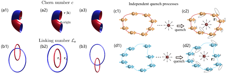
Figure 1: (a1)-(a3) Schematic several representative configurations of the extended QWZ model. The topology of the system can be determined by the times the torus $\mathbf{r\left(\mathbf{k}\right)}$ contains the origin which is represented by the green solid circle. The blue and red colors represent two sides of the surface. The potentials for panels (a1), (a2), and (a3) are $\mu=2,0,-3$, respectively, with the corresponding Chern numbers $c=1,0,-1$. For clarity, only the image of half of the Brillouin zone is shown. Other parameters are $\lambda_{1}=3$, $\lambda_{2}=1$, $\rho_{1}=3$, and $\rho_{2}=2$. (b1)-(b3) The Schematic representation of the two loops $\mathbf{r}_{1}$ and $\mathbf{r}_{2}$ defined in Eqs. (5) and (6). The two loops in (b) share the same parameters as the torus in (a) within the same column. The equivalence between the linking number $\mathcal{L}_{\mathbf{r}}$ and the Chern number $c$ enables the dynamical detection. (c) and (d) Schematic illustration of the independent quench processes. The red solid circle represents the origin, while the yellow and cyan arrows indicate two sets of Bloch vectors. Initially, the Bloch vector is prepared in the ground state of the prequench Hamiltonian and subsequently driven by the postquench Hamiltonian. The topology of the 2D model is determined by the behavior of the evolved Bloch vector.

II Model and double loops

We begin by introducing the two-band Bloch Hamiltonian in the form $h\left(\mathbf{k}\right)=\mathbf{r}\left(\mathbf{k}\right)\mathbf{\cdot\sigma,}$where $\mathbf{\sigma=}\left(\sigma_{x},\sigma_{y},\sigma_{z}\right)$ are Pauli matrices satisfying the Lie algebra commutation relations, and wave vector $\mathbf{k}=\left(k_{x},k_{y}\right)$ varies over the Brillouin zone (BZ) $k_{x},k_{y}\in\left(-\pi,\pi\right]$. The eigenvalues of the Hamiltonian are $\pm\left|\mathbf{r}\left(\mathbf{k}\right)\right|$, corresponding to the upper and lower bands, respectively, $h\left(\mathbf{k}\right)\left|u_{\pm}^{\mathbf{k}}\right\rangle=\pm\left|\mathbf{r}\left(\mathbf{k}\right)\right|\left|u_{\pm}^{\mathbf{k}}\right\rangle$. We note that the gap of $h\left(\mathbf{k}\right)$ closes when the absolute value of $\mathbf{r}\left(\mathbf{k}\right)$ equals zero. Matrix $h\left(\mathbf{k}\right)$ can serve as a core matrix of the crystalline system for non-interacting Hamiltonian, or Kitaev chain. In equilibrium paradigm, topological phase diagrams of this model can be characterized by Chern number [41, 42], for which the lower band is defined as,

$$c=\frac{1}{4\pi}\oint_{0}^{2\pi}\oint_{0}^{2\pi}\frac{\mathbf{r}}{\left|\mathbf{r}\right|^{3}}\cdot\left(\partial_{k_{x}}\mathbf{r}_{1}\mathbf{\times}\partial_{k_{y}}\mathbf{r}_{2}\right)\mathrm{d}k_{x}\mathrm{d}k_{y}.$$ (1)

It can also be interpreted as the number of times the surface traced by the end of $\mathbf{r}\left(\mathbf{k}\right)$ in the auxiliary space encloses the origin, as illustrated in Fig. 1(a).

In our paper, we focus on the condition that the vector $\mathbf{r}\left(\mathbf{k}\right)$ can be represented by two periodic vector functions, $\mathbf{r}_{1}$ and $\mathbf{r}_{2}$, with respect to the wave vectors $k_{x},k_{y}$ in the two directions,

$$\mathbf{r}\left(k_{x},k_{y}\right)=\mathbf{r}_{1}\left(k_{x}\right)-\mathbf{r}_{2}(k_{y}).$$ (2)

It is clear that $\mathbf{r}_{1}$ and $\mathbf{r}_{2}$ represent two loops in 3D auxiliary space. The gap closing $\left|\mathbf{r}\right|=0$ can be predicted by the crossing of them $\mathbf{r}_{1}\left(k_{x}\right)=\mathbf{r}_{2}(k_{y})$. This phenomenon inspires us to explore the Chern number characterized by $\mathbf{r}\left(\mathbf{k}\right)$ based on the trajectories of two loops. To this end, we introduce the corresponding linking number,

$$\mathcal{L}_{\mathbf{r}}=\frac{1}{4\pi}\oint_{{\ell}_{2}}\oint_{{\ell}_{1}}\frac{\mathbf{r}_{1}-\mathbf{r}_{2}}{\left|\mathbf{r}_{1}-\mathbf{r}_{2}\right|^{3}}\cdot\left(\mathrm{d}\mathbf{r}_{2}\times\mathrm{d}\mathbf{r}_{1}\right).$$ (3)

It can be readily verified that the linking number $\mathcal{L}_{\mathbf{r}}$ is equal to the Chern number $c$ defined in Eq. (1). This relation is the main result in Ref. [38] and serves as the foundation of our paper.

To describe this relation more concretely, we take the extended QWZ model as a representative example, whose Bloch Hamiltonian is expressed as,

$$\mathbf{r=}\left(\lambda_{x}\sin k_{x},\lambda_{y}\sin k_{y},\mu+\rho_{x}\cos k_{x}+\rho_{y}\cos k_{y}\right).$$ (4)

This model was recently realized by the University of Science and Technology of China and Peking University (USTC-PKU) group on a square Raman lattice [43]. In this setup, $\lambda$ and $\rho$ denote the spin-conserved and spin-flip hopping coefficients, respectively [44]. $\mu$ represents the Zeeman constant. Suddenly modulating the Zeeman constants $\mu$ can implement the quench dynamics. We can rewrite $\mathbf{r}$ in the form of $\mathbf{r}_{1}$ and $\mathbf{r}_{2}$,

$$\mathbf{r}_{1} = \left(\lambda_{x}\sin k_{x},0,\mu_{1}+\rho_{x}\cos k_{x}\right),$$ (5)

$$\mathbf{r}_{2} = \left(0,-\lambda_{y}\sin k_{y},\mu_{2}-\rho_{y}\cos k_{y}\right),$$ (6)

where $\mu_{1}-\mu_{2}=\mu$. Here, $\mathbf{r}_{1}$ and $\mathbf{r}_{2}$ represent two ovals in the $xz$ and $yz$ planes, respectively, with centers at $\left(0,0,\mu_{1}\right)$ and $\left(0,0,\mu_{2}\right)$. We plot several representative configurations in Fig. 1(a) and (b) for $\lambda_{x}=\rho_{x}=3$, $\lambda_{y}=1$, and $\rho_{y}=2$, while varying the potential $\mu$ for the panels in different columns. The schematics illustrate that the Chern number can be easily obtained from the geometrical configuration of the two loops. Compared to the direct calculation of the Chern number from the Berry connection, These relations offer a convenient demonstration of the system’s topological characteristics. In the following, we present an intuitive application.

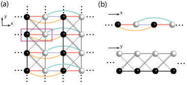
Figure 2: (a) Schematic of the 2D model defined in Eq. (7). The unit cell consists of two sublattices, A (black) and B (white), as indicated inside the red rectangle. The colored bonds represent the interaction along the $x$ direction, while the black bonds, with varying structures, indicate the interactions along the $y$ direction. (b) Schematic of two independent chains corresponding to the 2D system in (a), as demonstrated in Eqs. (20) and (23), respectively. The colored bonds are used to construct one chain, and the black bonds form the other.

III Hidden Chern number of two chains

Based on the above analysis, we attempt to reveal the topological properties for a class of 2D systems using two 1D chains. These 2D systems comprise of two sublattices, $A$ and $B$ with the coordinates for the unit cell denoted as $(l,j)$, $1\leq l,j\leq N$, and can be realized in many experimental platforms for the topological insulators [45, 46]. We use $a_{l,j}^{\dagger},b_{l,j}^{\dagger}$ ($a_{l,j},b_{l,j}$) to represent the creation (annihilation) operators for the sublattices $A$ and $B$. For the periodic boundary condition considered in this paper, we set $a_{l+N,j+N}=a_{l,j}$ and $b_{l+N,j+N}=b_{l,j}$. The general schematic illustration is plotted in Fig. 2(a). The coupling between the two unit cells occurs exclusively along the $x$ or $y$ directions, represented by colored and black bonds, respectively. In the $x$ direction, different colors indicate varying coupling strengths, while the distinct structures of the black bonds denote different coupling strengths in the $y$ direction. The general form of the Hamiltonian in the real space is,

$$H=\sum_{l,j,n}H_{l,j,n}^{x}+H_{l,j,n}^{y},$$ (7)

where $H_{l,j,n}^{x}$ ($H_{l,j,n}^{y}$) denotes the $n$th nearest neighbor coupling along $x$ ($y$) direction,

$$H_{l,j,n}^{x} = \left(a_{l,j}^{\dagger},b_{l,j}^{\dagger}\right)\mathbf{d}_{n}^{x}\cdot\mathbf{\sigma}\left(\begin{array}[]{c}a_{l+n,j}\\ b_{l+n,j}\end{array}\right)+\mathrm{H.c.,}$$ (10)

$$H_{l,j,n}^{y} = \left(a_{l,j}^{\dagger},b_{l,j}^{\dagger}\right)\mathbf{d}_{n}^{y}\cdot\mathbf{\sigma}\left(\begin{array}[]{c}a_{l,j+n}\\ b_{l,j+n}\end{array}\right)+\mathrm{H.c..}$$ (13)

The vector components of $\mathbf{d}$ can be real or complex. Applying the Fourier transformation to the two sublattices,

$$a_{\mathbf{k}} = \frac{1}{N}\sum_{l,j}e^{-i\mathbf{k\cdot r}}a_{l,j},$$ (14)

$$b_{\mathbf{k}} = \frac{1}{N}\sum_{l,j}e^{-i\mathbf{k\cdot r}}b_{l,j}.$$ (15)

with the wave vector $\mathbf{k}=\left(k_{x},k_{y}\right)$, we can rewrite the lattice Hamiltonian in the momentum space,

$$H=\sum_{\mathbf{k}}\psi_{\mathbf{k}}^{\dagger}h\left(\mathbf{k}\right)\psi_{\mathbf{k}}.$$ (16)

Here the basis is $\psi_{\mathbf{k}}=\left(a_{\mathbf{k}},b_{\mathbf{k}}\right)^{T}$. The Bloch Hamiltonian is a $2\times 2$ matrix $h\left(\mathbf{k}\right)=\mathbf{r}\left(\mathbf{k}\right)\mathbf{\cdot\sigma}$ and the vector $\mathbf{r}\left(\mathbf{k}\right)$ takes the form

$$\mathbf{r}\left(\mathbf{k}\right)=\sum_{n}\exp\left(ik_{x}n\right)\mathbf{d}_{n}^{x}+\exp\left(ik_{y}n\right)\mathbf{d}_{n}^{y}+\mathrm{c.c.}.$$ (17)

Simultaneously, we can also construct two one-dimensional chains using the coupling in the two directions, respectively, e.g.,

$$H_{1} = \sum_{l,n}\left(a_{l,1}^{\dagger},b_{l,1}^{\dagger}\right)\mathbf{d}_{n}^{x}\cdot\mathbf{\sigma}\left(\begin{array}[]{c}a_{l+n,1}\\ b_{l+n,1}\end{array}\right)+\mathrm{H.c.},$$ (20)

$$H_{2} = -\sum_{j,n}\left(a_{1,j}^{\dagger},b_{1,j}^{\dagger}\right)\mathbf{d}_{n}^{y}\cdot\mathbf{\sigma}\left(\begin{array}[]{c}a_{1,j+n}\\ b_{1,j+n}\end{array}\right)+\mathrm{H.c.,},$$ (23)

as illustrated in Fig. 2(b). The corresponding Bloch Hamiltonian $h_{\alpha}(k)=\mathbf{r}_{\alpha}(k)\mathbf{\cdot\sigma}$, $\alpha=1,2$ can be obtained easily based on the Fourier transformation in 1D and it is easy to verify that $\mathbf{r\left(\mathbf{k}\right)=r}_{1}(k_{x})-\mathbf{r}_{2}(k_{y})$.

Based on the result in the previous section, we can directly conclude that the topological phase of the 2D model in Eq. (7) can be completely classified according to the linking number of two loops, $\mathbf{r}_{1}$ and $\mathbf{r}_{2}$, which are abstracted from each chain individually. This description of the topological system is more feasible experimentally, as it eliminates the need to fabricate a 2D topological structure, allowing us to focus solely on two 1D chains.

IV Nonequilibrium steady vector

In this section, we introduce a scheme to predict the topological properties of 2D models via two independent quench processes driven by the 1D chains, which is the primary focus of our work. An extensively studied approach to analogize the quantum phase transition is known as dynamical quantum phase transition (DQPT) [24, 25]. However, the exact nature of the non-analyticity in 2D remains unclear currently. Although several schemes [36, 26] are shown to be applicable in 2D, it is worth investigating whether the topological properties of the 2D model $H$ in Eq. (7) can be effectively captured by the quench processes driven by $H_{1}$ and $H_{2}$, given the challenges of inducing the complex dynamics required for topological phases in high-dimensional systems.

We thus consider the following quench process: Initially, we prepare two sets of tensor product states, $\left|\psi_{\alpha}(0)\right\rangle=\prod_{k}\left|\psi_{\alpha}^{k}(0)\right\rangle,\alpha=1,2$. $\left|\psi_{\alpha}^{k}(0)\right\rangle$ represents the eigenstate of $\sigma_{z}$ with eigenvalue $-1$. These two sets of initial states contain no information about the driven Hamiltonian. Next, we drive them by $H_{\alpha}$ for any given time $t$ and every state will evolve as follows,

$$\left|\psi_{\alpha}(t)\right\rangle=\exp\left(-iH_{\alpha}t\right)\left|\psi_{\alpha}(0)\right\rangle,\alpha=1,2.$$ (24)

It is easy to check that the evolved state remains a tensor product state, i.e., $\left|\psi_{\alpha}(t)\right\rangle=\prod_{k}\exp\left[-ih_{\alpha}(k)t\right]\left|\psi_{\alpha}^{k}(0)\right\rangle$ . We can calculate the interaction-free Bloch vector,

$$\mathbf{n}_{\alpha}(k,t)=\left\langle\psi_{a}^{k}(t)\right|\mathbf{\sigma}\left|\psi_{a}^{k}(t)\right\rangle,$$ (25)

for each momentum space over time. The time evolution of the Bloch vector can be observed as precession along the direction of $\mathbf{r}_{\alpha}(k,t)$ [36]. A schematic illustration of the quench process is plotted in Fig. 1(c) and (d). Initially, the endpoints of Bloch vectors $\mathbf{n}_{\alpha}(k,t)$ converge at the south pole on the Bloch sphere, i.e., $\mathbf{n}_{1}(0)=\mathbf{n}_{2}(0)=\left(0,0,-1\right)$. As time progresses, these endpoints will diverge and trace out two instantaneous loops on the Bloch sphere. The dynamical behavior allows us to calculate the following three variables: (1) The frequency of precession, denoted as $\omega_{\alpha}^{k}$; (2) The average Bloch vector, given by the formula

$$\mathbf{\bar{n}}_{\alpha}(k,T)=\frac{1}{T}\int_{0}^{T}\mathbf{n}_{\alpha}(k,\tau)\mathrm{d}\tau\text{;}$$ (26)

(3) The sign $\rho$ of the precession rate, where positive values indicate a counterclockwise direction and negative values to indicate a clockwise direction, as observed from the center of precession. We can delineate two time-dependent loops based on the above three variables,

$$\mathbf{l}_{\alpha}\left(k,T\right)=\frac{\rho\omega_{\alpha}^{k}\mathbf{\bar{n}}_{\alpha}(k,T)}{2\left|\mathbf{\bar{n}}_{\alpha}(k,T)\right|},$$ (27)

and calculate the corresponding linking number

$$\mathcal{L}_{\mathbf{l}}(T)=\frac{1}{4\pi}\oint\oint\frac{\mathbf{l}_{1}(T)-\mathbf{l}_{2}(T)}{\left|\mathbf{l}_{1}(T)-\mathbf{l}_{2}(T)\right|^{3}}\cdot\left[\mathrm{d}\mathbf{l}_{2}(T)\times\mathrm{d}\mathbf{l}_{1}(T)\right].$$ (28)

On the one hand, over an extended period, $T\rightarrow\infty$, the integration in Eq. (26) yields a steady value, given by,

$$\mathbf{\bar{n}}_{\alpha}(k) = \lim_{T\rightarrow\infty}\mathbf{\bar{n}}_{\alpha}(k,T)$$ (29)

$$= -\mathbf{\hat{r}}_{\alpha}\left(k\right)\left(\mathbf{\hat{r}}_{\alpha}\left(k\right)\cdot\widehat{z}\right).$$ (30)

The vector $\mathbf{\hat{r}}_{\alpha}\left(k\right)$ denotes the direction of the Bloch Hamiltonian $\mathbf{r}_{\alpha}(k)$, $\mathbf{\hat{r}}_{\alpha}\left(k\right)=\mathbf{r}_{\alpha}\left(k\right)/\left|\mathbf{r}_{\alpha}\left(k\right)\right|$. On the other hand, it is also straightforward to demonstrate that the precession frequency $\omega_{\alpha}^{k}$ is equal to the bandwidth $2\left|\mathbf{r}_{\alpha}\left(k\right)\right|$. Based on the above analysis, we can verify that the trajectory of $\mathbf{l}_{\alpha}\left(k,T\right)$ will become steady as time approaches infinity and converges to $\mathbf{r}_{\alpha}\left(k\right)$. The non-equilibrium steady behavior of $\mathbf{l}_{\alpha}\left(k,T\right)$ leads to the equivalence of the linking number defined in Eq. (3) and Eq. (28), such that $\lim_{T\rightarrow\infty}\mathcal{L}_{\mathbf{l}}(T)=\mathcal{L}_{\mathbf{r}}$. In the following, we perform the numerical simulation based on the extended QWZ model.

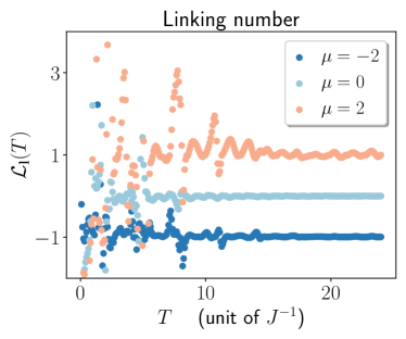
Figure 3: Numerical simulations of the linking number defined in Eq. (28) as a function of time $T$ for case $N=50$ in various topological regions. We can see that the linking number undergoes damped oscillation around a stable value that matches the Chern number. Other parameters are $\lambda_{x}=\rho_{x}=3$, $\lambda_{y}=1$, and $\rho_{y}=2$.

V Extended QWZ model

In this section, we consider the extended QWZ model which has been introduced in Sec. II to illustrate our scheme. To simplify the discussion, we select the same parameters in Fig. 1(a) and (b) and the phase diagram is clear: $c=0$, for $\left|\mu\right|<1$ or $\left|\mu\right|>5$, and $c=\pm 1$ for $1<\pm\mu<5$.

We perform numerical simulation of the quench processes driven by the Bloch Hamiltonian in Eqs. (5) and (6) for $\mu_{1}=\mu$ and $\mu_{2}=0$, and calculate $\mathcal{L}_{\mathbf{l}}(T)$ the as a function of $T$. Here, the initial state $\left|\psi_{\alpha}^{k}(0)\right\rangle=\left(0,1\right)^{T}$ can be prepared as the ground state for infinite potential, $\mu_{1}\rightarrow\infty$ and $\mu_{2}\rightarrow\infty$. It is accessible for the experiment in Ref. [43] as we can modulate the Zeeman constants flexibly. The result is plotted in Fig. 3.

Initially, we find that the value of $\mathcal{L}_{\mathbf{l}}(T)$ is not an integer during the early stages and oscillates irregularly. The reasons are as follows: Referring to Eq. (27), several wave vectors near the critical value $k_{c}$ can lead to unpredictable and non-negligible errors in numerical simulation. This critical value $k_{c}$ is defined by the condition $\mathbf{\hat{r}}_{\alpha}\left(k_{c}\right)\cdot\widehat{z}=0$ and is also the source of non-analytic behavior in DQPT. Traditionally, improving the accuracy of the simulation requires increasing the length $N$, reducing the time interval $\delta t$ in dynamic simulations, adjusting data types, and so on. These adjustments will inevitably lead to an increase in simulation duration.

However, as time increases, the amplitudes of the oscillations continue to decrease for various values of $\mu$ due to the integral in Eq. (26). $\mathcal{L}_{\mathbf{l}}(T)$ tends to a steady value and eventually becomes the same as the Chern number, thereby illustrating the topological information of the QWZ model. The results indicate that our dynamical method effectively conserves computational resources in numerical simulations. Moreover, this approach may also facilitate experimental measurements by offering a simplified and experimentally accessible way to evaluate the topological features of 2D systems.

VI Summary and discussion

In summary, we elucidate the topological properties of 2D model $\mathbf{r}(k_{x},k_{y})$ through two 1D chains, $\mathbf{r}_{1}(k)$ and $\mathbf{r}_{2}(k)$, using a quantum quench dynamics approach. we find that the equilibrium topological phase diagram of the 2D model can be accurately predicted by the linking number of these corresponding 1D chains. This equivalence inspires us to use a sudden quench approach based on the two 1D chains to determine the Chern number of the 2D model, which potentially facilitates experimental measurements. Based on the exact solutions and numerical simulations, we observe that the steady linking number of the two loops $\mathbf{l}_{1}\left(k,T\right)$ and $\mathbf{l}_{2}\left(k,T\right)$ generated by the quench dynamics displays distinct behaviors depending on the topological phase of the system. The QWZ model is employed as an example to illustrate the scheme. These findings offer valuable insights into the dynamical detection of the topological phases in 2D models using corresponding 1D chains. In future research, we aim to extend our investigation to multi-band and three-dimensional models and broaden our understanding of non-equilibrium behaviors.

References

- Monroe et al. [2021] C. Monroe, W. C. Campbell, L.-M. Duan, Z.-X. Gong, A. V. Gorshkov, P. W. Hess, R. Islam, K. Kim, N. M. Linke, G. Pagano, et al., Reviews of Modern Physics 93, 025001 (2021).
- Blatt and Roos [2012] R. Blatt and C. F. Roos, Nature Physics 8, 277 (2012).
- Schreiber et al. [2015] M. Schreiber, S. S. Hodgman, P. Bordia, H. P. Lüschen, M. H. Fischer, R. Vosk, E. Altman, U. Schneider, and I. Bloch, Science 349, 842 (2015).
- Bernien et al. [2017] H. Bernien, S. Schwartz, A. Keesling, H. Levine, A. Omran, H. Pichler, S. Choi, A. S. Zibrov, M. Endres, M. Greiner, et al., Nature 551, 579 (2017).
- Choi et al. [2017] S. Choi, J. Choi, R. Landig, G. Kucsko, H. Zhou, J. Isoya, F. Jelezko, S. Onoda, H. Sumiya, V. Khemani, et al., Nature 543, 221 (2017).
- Wallraff et al. [2004] A. Wallraff, D. Schuster, A. Blais, L. Frunzio, R.-S. Huang, J. Majer, S. Kumar, S. Girvin, and R. Schoelkopf, arXiv preprint cond-mat/0407325 (2004).
- Xu et al. [2020] K. Xu, Z.-H. Sun, W. Liu, Y.-R. Zhang, H. Li, H. Dong, W. Ren, P. Zhang, F. Nori, D. Zheng, et al., Science advances 6, eaba4935 (2020).
- Chang et al. [2018] D. Chang, J. Douglas, A. González-Tudela, C.-L. Hung, and H. Kimble, Reviews of Modern Physics 90, 031002 (2018).
- Ye et al. [2008] J. Ye, H. Kimble, and H. Katori, science 320, 1734 (2008).
- Raimond et al. [2001] J.-M. Raimond, M. Brune, and S. Haroche, Reviews of Modern Physics 73, 565 (2001).
- Gring et al. [2012] M. Gring, M. Kuhnert, T. Langen, T. Kitagawa, B. Rauer, M. Schreitl, I. Mazets, D. A. Smith, E. Demler, and J. Schmiedmayer, Science 337, 1318 (2012).
- Neyenhuis et al. [2017] B. Neyenhuis, J. Zhang, P. W. Hess, J. Smith, A. C. Lee, P. Richerme, Z.-X. Gong, A. V. Gorshkov, and C. Monroe, Science advances 3, e1700672 (2017).
- Smith et al. [2016] J. Smith, A. Lee, P. Richerme, B. Neyenhuis, P. W. Hess, P. Hauke, M. Heyl, D. A. Huse, and C. Monroe, Nature Physics 12, 907 (2016).
- Choi et al. [2016] J.-Y. Choi, S. Hild, J. Zeiher, P. Schauß, A. Rubio-Abadal, T. Yefsah, V. Khemani, D. A. Huse, I. Bloch, and C. Gross, Science 352, 1547 (2016).
- Zhang et al. [2017a] J. Zhang, P. W. Hess, A. Kyprianidis, P. Becker, A. Lee, J. Smith, G. Pagano, I.-D. Potirniche, A. C. Potter, A. Vishwanath, et al., Nature 543, 217 (2017a).
- Zhang et al. [2017b] J. Zhang, G. Pagano, P. W. Hess, A. Kyprianidis, P. Becker, H. Kaplan, A. V. Gorshkov, Z.-X. Gong, and C. Monroe, Nature 551, 601 (2017b).
- Jurcevic et al. [2017] P. Jurcevic, H. Shen, P. Hauke, C. Maier, T. Brydges, C. Hempel, B. Lanyon, M. Heyl, R. Blatt, and C. Roos, Physical review letters 119, 080501 (2017).
- Jotzu et al. [2014] G. Jotzu, M. Messer, R. Desbuquois, M. Lebrat, T. Uehlinger, D. Greif, and T. Esslinger, Nature 515, 237 (2014).
- Wu et al. [2016] Z. Wu, L. Zhang, W. Sun, X.-T. Xu, B.-Z. Wang, S.-C. Ji, Y. Deng, S. Chen, X.-J. Liu, and J.-W. Pan, Science 354, 83 (2016).
- Lohse et al. [2016] M. Lohse, C. Schweizer, O. Zilberberg, M. Aidelsburger, and I. Bloch, Nature Physics 12, 350 (2016).
- Tai et al. [2017] M. E. Tai, A. Lukin, M. Rispoli, R. Schittko, T. Menke, D. Borgnia, P. M. Preiss, F. Grusdt, A. M. Kaufman, and M. Greiner, Nature 546, 519 (2017).
- Kennedy et al. [2015] C. J. Kennedy, W. C. Burton, W. C. Chung, and W. Ketterle, Nature Physics 11, 859 (2015).
- Fläschner et al. [2018] N. Fläschner, D. Vogel, M. Tarnowski, B. Rem, D.-S. Lühmann, M. Heyl, J. Budich, L. Mathey, K. Sengstock, and C. Weitenberg, Nature Physics 14, 265 (2018).
- Heyl et al. [2013] M. Heyl, A. Polkovnikov, and S. Kehrein, Physical review letters 110, 135704 (2013).
- Heyl [2018] M. Heyl, Reports on Progress in Physics 81, 054001 (2018).
- Wang et al. [2017] C. Wang, P. Zhang, X. Chen, J. Yu, and H. Zhai, Physical review letters 118, 185701 (2017).
- Heyl [2015] M. Heyl, Physical Review Letters 115, 140602 (2015).
- Shi et al. [2022] Y. Shi, K. Zhang, and Z. Song, Physical Review B 106, 184505 (2022).
- Altland and Zirnbauer [1997] A. Altland and M. R. Zirnbauer, Physical Review B 55, 1142 (1997).
- Kitaev [2001] A. Y. Kitaev, Physics-uspekhi 44, 131 (2001).
- Soori [2024] A. Soori, arXiv preprint arXiv:2403.02266 (2024).
- Decker and Karrasch [2024] K. Decker and C. Karrasch, arXiv preprint arXiv:2402.12897 (2024).
- Malard and Brandão [2024] M. Malard and D. S. Brandão, arXiv preprint arXiv:2403.01588 (2024).
- Silva et al. [2024] E. Silva, R. B. Ribeiro, H. Caldas, and M. A. Continentino, Physical Review B 109, 134503 (2024).
- Starchl and Sieberer [2022] E. Starchl and L. M. Sieberer, Physical Review Letters 129, 220602 (2022).
- Shi et al. [2023] Y. Shi, X. Zhang, and Z. Song, arXiv preprint arXiv:2311.08056 (2023).
- Kosior and Heyl [2024] A. Kosior and M. Heyl, Physical Review B 109, L140303 (2024).
- Yang and Song [2020] X. Yang and Z. Song, Physical Review B 102, 195112 (2020).
- Qi et al. [2006] X.-L. Qi, Y.-S. Wu, and S.-C. Zhang, Physical Review B—Condensed Matter and Materials Physics 74, 085308 (2006).
- Bernevig et al. [2006] B. A. Bernevig, T. L. Hughes, and S.-C. Zhang, science 314, 1757 (2006).
- Qi and Zhang [2011] X.-L. Qi and S.-C. Zhang, Reviews of modern physics 83, 1057 (2011).
- Cho and Moore [2011] G. Y. Cho and J. E. Moore, Physical Review B—Condensed Matter and Materials Physics 84, 165101 (2011).
- Yi et al. [2019] C.-R. Yi, L. Zhang, L. Zhang, R.-H. Jiao, X.-C. Cheng, Z.-Y. Wang, X.-T. Xu, W. Sun, X.-J. Liu, S. Chen, et al., Physical review letters 123, 190603 (2019).
- Ma et al. [2023] Y. Ma, X. Li, Y. Wang, S. Zhao, G. Xiong, and T. Sun, Physical Review B 108, 075128 (2023).
- Mittal et al. [2018] S. Mittal, E. A. Goldschmidt, and M. Hafezi, Nature 561, 502 (2018).
- Hofmann et al. [2019] T. Hofmann, T. Helbig, C. H. Lee, M. Greiter, and R. Thomale, Physical review letters 122, 247702 (2019).