Arrested development and traveling waves of active suspensions
in nematic liquid crystals

Abstract

Active particles in anisotropic, viscoelastic fluids experience competing stresses which guide their trajectories. An aligned suspension of particles can trigger a hydrodynamic bend instability, but the elasticity of the fluid can drive particle orientations back towards alignment. To study these competing effects, we examine a dilute suspension of active particles in an Ericksen-Leslie model nematic liquid crystal. For small active Ericksen number or particle concentration the suspension settles to an equilibrium state with uniform alignment. Beyond a critical active Ericksen number or particle concentration the suspension instead can buckle into a steady flowing state. Rather than entering the fully developed roiling state observed in isotropic fluids, however, the development is arrested by fluid elasticity. Arrested states of higher wavenumber emerge at yet higher values of active Ericksen number. If the active particles are motile, traveling waves emerge, including a traveling, oscillatory ‘thrashing’ state. Moment equations are derived, compared to kinetic theory simulations, and analyzed in asymptotic limits which admit exact expressions for the traveling wave speed and both particle orientation and director fields in the arrested state.

Active particles in viscous fluids, from motile microorganisms to molecular-motor-driven biofilaments, generate stresses on the environment which can drive flow and affect particle orientational order. Biological fluids introduce additional complexity. Mucus, for instance, is anisotropic when sheared [1], which can rectify and otherwise affect microorganism transport [2, 3, 4, 5]. Viscoelasticity and shear-dependent viscosity, generic in biological settings, also affect motility [6, 7, 8]. Liquid crystals (LCs) [9, 10] have been used to probe the role of complex fluid stresses on bacterial transport in a more controlled setting [11, 12, 13]. At high bacterial concentrations, collective behavior is observed [14] which is distinguishable from such behaviors in isotropic viscous fluids.

In a Newtonian fluid, orientational alignment can emerge due to hydrodynamic interactions alone [15], but such uniformly aligned states are unstable to a bend instability [16], leading to chaotic dynamics [17, 18, 19, 20]. When swimming through a nematic LC, however, microorganisms can be confined by elastic stresses to swim along the director axis [21, 11, 12, 22, 23, 24, 25, 26], depending on the anchoring conditions [27], which can affect the nature of the bend instability and the nonlinear dynamics so triggered.

Particle motility and/or the concentration of active particles in an otherwise passive medium introduce additional collective behaviors. Driven actin filaments [28], Quincke rollers [29], and swimming spermatozoa [30] can all exhibit wave-like dynamics, even in isotropic fluids. Density waves in active media have been found in models ranging from the Viscek and Toner-Tu–type continuum models [31, 32, 33, 34, 35, 18, 36], to models incorporating hydrodynamic particle interactions [37, 38]. Solitary waves have also been observed in these models and in experiments [39, 28], where large particle concentration and system size can result in the formation of particle bands.

Experiments using a dilute suspension of microorganisms swimming through LCs have shown a change from individual rectified motion to the formation of a wave-like jet of swimming particles [40]. The wave dynamics in this experiment suggest a balance between active and elastic stresses. The behavior of a LC hosting a suspension of active particles (a ‘living liquid crystal’ [11]) thus depends on the particle concentration.

In related active nematics, the constituents provide both nematic order and active stresses [41, 42, 43]. Active nematics support steady streaming states and regions of hysteresis [44, 45, 46, 47, 48, 49, 50, 51], and interfacial wave propagation [52], which depend on the nature of stress generation (extensile or contractile), and flow aligning/tumbling properties. These steady streaming states, in which fluid elasticity arrests further instability development, were studied recently by Lavi et al. [53]. High wavenumber labyrinthine patterns emerged at large active stresses. Pseudo-defect formation was also explored, and defects were found to destabilize arrested states into active turbulent states. A natural question arises: in what settings might such states emerge in living liquid crystals?

In this letter, we present a model for a dilute suspension of active particles in a nematic liquid crystal. An active Ericksen number, comparing active stresses to elastic fluid stresses, is used to explore a wide range of related systems. We observe bifurcations in the dynamics as either the particle concentration or the active Ericksen number is increased for immotile extensile-stress-generating (‘pusher’) particles, first from uniform alignment and no flow, to the development of an arrested state with steady streaming, and then to arrested states of higher wavenumber. Analytical results are provided in asymptotic regimes, including stability criteria which depend on the material properties of the LC and surface anchoring strength. If the particles are motile, arrested states can translate at a finite wavespeed, or even express a periodic ‘thrashing’ mode. These wavespeeds are also derived in the limit of small particle swimming speed.

Model: The particles are modeled as prolate ellipsoids with major and minor axis lengths $2a$ and $2b$, volume $v=4\pi ab^{2}/3$ and surface area $S$, residing in a cubic domain of volume $V=L^{3}$. The number of particles, $N$, is constant, and the particle volume fraction is $\phi:=Nv/V$. The number density of particles is written as $\psi^{*}(a\bm{x},\bm{p},Tt)=NL^{-3}\psi(\bm{x},\bm{p},t)$, where $a\bm{x}$ is the spatial position and $Tt$ is time ($T$ is defined below), and $\bm{x}\in[0,\mathcal{L}]^{3}$ with $\mathcal{L}:=L/a$. The particle concentration is given by $c^{*}(a\bm{x},Tt)=NL^{-3}c(\bm{x},t)$, where $c=\int_{\mathbb{S}^{2}}\psi(\bm{x},\bm{p},t)\,d\bm{p}$.

The particles are assumed to be much larger than the LC molecules (Fig. 1a) - a Type VI system in the language of Ref. [8]. The LC dynamics are treated using the Ericksen-Leslie model (in the one-constant approximation), with elastic energy density $(K/2a^{2})|\nabla\bm{n}|^{2}$, $K$ the Frank elastic constant, and $\nabla=\partial_{\bm{x}}$ [54, 9]. Tangential anchoring conditions of strength $W$ are assumed on the LC/particle boundaries [27]. Denoting the local LC orientation by $\bm{n}$, the bulk energy density is modeled as $(K/a^{2})\mathcal{F}$, where (see [55])

$$\mathcal{F}=\frac{1}{2}|\nabla\bm{n}|^{2}+\frac{\mathcal{W}}{2}\int_{\mathbb{S}^{2}}\psi(\bm{x},\bm{p},t)\left(1-(\bm{n}\cdot\bm{p})^{2}\right)\,d\bm{p}.$$ (1)

A penalty has been assigned on misaligned particles, and $\mathcal{W}=SW/(aK)$ is the dimensionless anchoring strength [56, 57, 58]. Variations in the molecular position and orientation produces a stress $(K/a^{2})\bm{\sigma}_{r}(\bm{x},t)$, where

$$\bm{\sigma}_{r}=-\nabla\bm{n}\cdot\nabla\bm{n}^{T}-\frac{\lambda}{2}(\bm{n}\bm{h}+\bm{h}\bm{n})+\frac{1}{2}(\bm{n}\bm{h}-\bm{h}\bm{n}),$$ (2)

with $\bm{h}=(\bm{\mathrm{I}}-\bm{n}\bm{n})\cdot\left[\nabla^{2}\bm{n}+\mathcal{W}\bm{n}\cdot(c\bm{\mathrm{D}})\right]$, and $\lambda$ the tumbling parameter [55, 54, 9]. Here and elsewhere, $\bm{n}\bm{h}$ and similar terms are dyadic products.

Each particle imposes a force dipole of strength $\sigma_{0}$ on the surrounding fluid, resulting in a locally averaged active stress $\sigma_{0}c\bm{\mathrm{D}}$ [59, 15]. Choosing now the timescale, $T=\mu a^{2}/K$, the fluid velocity is denoted by $\bm{u}^{*}(a\bm{x},Tt)=K(\mu a)^{-1}\bm{u}(\bm{x},t)$, where $\mu$ is the solvent viscosity (anisotropic viscosity coefficients are neglected). Dimensionless momentum balance is given by

$$-\nabla p+\nabla^{2}\bm{u}+\nabla\cdot\left(\bm{\sigma}_{r}+\mbox{Er}_{a}\phi c\bm{\mathrm{D}}\right)=\bm{0},$$ (3)

with $p$ the pressure, a Lagrange multiplier which enforces continuity, $\nabla\cdot\bm{u}=0$. We have here defined the active Ericksen number, $\mbox{Er}_{a}:=\sigma_{0}a^{2}/(vK)$, which scales linearly with the active stress and inversely with LC elasticity [60]. If $\mbox{Er}_{a}<0$, the particles are extensile ‘pushers’, and with $\mbox{Er}_{a}>0$, they are contractile ‘pullers’.

The director field dynamics are given by

$$\frac{\mbox{D}\bm{n}}{\mbox{D}t}=(\bm{\mathrm{I}}-\bm{n}\bm{n})\cdot\left(\bm{n}\cdot\nabla\bm{u}+\frac{1}{\gamma}\bm{h}\right),$$ (4)

where $\mu\gamma$ is the rotational viscosity [55, 54, 9]. Conservation of the total number of active particles is expressed by a Smoluchowski equation for $\psi$ [61],

$$\psi_{t}+\nabla_{\bm{x}}\cdot(\dot{\bm{x}}\psi)+\nabla_{\bm{p}}\cdot(\dot{\bm{p}}\psi)=0,$$ (5)

where $\nabla_{\bm{p}}=(\bm{\mathrm{I}}-\bm{p}\bm{p})\cdot(\partial/\partial\bm{p})$, and $\dot{\bm{x}}$ and $\dot{\bm{p}}$ are particle translational and rotational velocities, modeled as

$$\dot{\bm{x}}=\bm{u}+\mathcal{V}_{0}\bm{p}-D\displaystyle\frac{\nabla_{\bm{x}}\psi}{\psi},$$ (6)

$$\dot{\bm{p}}=(\bm{\mathrm{I}}-\bm{p}\bm{p})\cdot\left[\bm{p}\cdot\nabla\bm{u}+\displaystyle\frac{\mathcal{W}}{\eta}(\bm{n}\cdot\bm{p})\bm{n}\right]-d\displaystyle\frac{\nabla_{\bm{p}}\psi}{\psi}.$$ (7)

With $V_{0}^{*}$, $D^{*}$, and $d^{*}$ the dimensional swimming speed, translational diffusivity, and rotational diffusivity, their dimensionless counterparts used above are $\mathcal{V}_{0}=\mu aV_{0}^{*}/K$, $D=\mu D^{*}/K$, and $d=\mu a^{2}d^{*}/K$. The moment acting on the LC by misaligned particles is balanced above by a corresponding torque $-SW\bm{n}\cdot\bm{p}$ on each particle, affecting orientation via a near-alignment rotational drag with coefficient $\eta$.

The system is governed by the dimensionless groups $(\mathcal{L},\mbox{Er}_{a},\mathcal{W},\mathcal{V}_{0},\gamma,D,d,\eta,\lambda)$. Characteristic values can be determined for B. subtilis cells in DSCG [62]. Assuming a domain with dimensions $\mathcal{L}=50$, we find $\mbox{Er}_{a}\approx 1-20$, $\mathcal{W}\approx 0.5-5$, $\mathcal{V}_{0}\approx 0.06$, $\gamma\approx 10^{-4}$, $D,d\approx 10^{-5}$, $\eta\approx 4$, and we fix $\lambda=1$ [55].

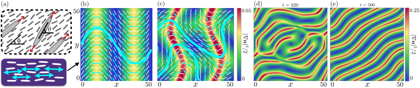
Figure 1: (a) Individual elongated particles with orientation $\bm{p}=(\cos\theta,\sin\theta)$ immersed in a liquid crystal (LC) with director field $\bm{n}=(\cos\Phi,\sin\Phi)$. (b) The first arrested flowing state ($\mbox{Er}_{a}=-8$, $\mathcal{W}=20$) from simulations using the full kinetic theory. White lines show the LC direction, cyan double arrows show the active particle orientations, and the background color shows the bulk LC elastic energy. One integral curve of the active particle field is also shown. The fluid velocity is everywhere in the vertical direction, and largest in magnitude in the regions of large LC bending (i.e. fluid flows drive local bending and high elastic energy). See Movie 2. (c) The second arrested state ($\mbox{Er}_{a}=-16$) is fully two dimensional, following a secondary bifurcation. Flows again drive regions of high LC bending, but in more focused regions. See Movie 3. (d) Dynamics with large extensile activity, $\mbox{Er}_{a}=-50$, and moderate anchoring strength, $\mathcal{W}=1$, using the full kinetic theory. For short times, the high wavenumber distortions and pseudo-defects are similar to the arrested labyrinthine states in active nematics. (e) At longer times the system relaxes towards a ‘one-dimensional’ arrested state as in (b).

Simulations: We consider confinement to motion in two dimensions $(x,y)$ and invariance in the third dimension, writing $\bm{p}=(\cos\theta,\sin\theta,0)$ and $\bm{n}=(\cos\Phi,\sin\Phi,0)$ (Fig. 1a). Simulations of Eqs. (3), (4) and (5) are performed using a pseudospectral method with $128^{3}$ Fourier modes and dealiasing [63, 64]; time-stepping is performed using an integrating factor method, along with a second-order accurate Adams-Bashforth scheme [63, 64].

We begin by considering immotile particles in the limit of small active Ericksen number, where elastic stresses dominate active stresses. For generic initial conditions in both particle concentration and orientation, the system rapidly stabilizes to a uniform LC orientation with active particle alignment in the LC direction. Diffusive spreading then leads to a constant concentration field and zero fluid velocity (see Movie 1).

Beyond a critical active Ericksen number or particle concentration, the classical bend instability of active particles overcomes the stabilizing LC elasticity. With a nearly uniform concentration of active particles in near-alignment with a uniform LC orientation field, a long-wave instability is triggered in both the particle and LC orientation fields. However, rather than continuing on to a fully developed, dynamic roiling state, like those seen in Newtonian fluids [17], LC elasticity arrests further growth and the system relaxes to a steady flowing state (as in Refs. [44, 45, 65, 53]), evocative of the classical Fréedericksz transition in nematic LCs [9, 10].

Figure 1b shows such a steady flowing state, with background color indicating the stored bulk LC elastic energy, $|\nabla\bm{n}|^{2}/2$, computed using $(\mbox{Er}_{a},\phi,\mathcal{W},\gamma,\eta,\lambda,D,d)=(-8,0.02,20,0.1,1,1,1,0.1)$ and random initial data. The velocity field is everywhere vertical and fastest in the region of high LC bending. A solid curve shows an integral curve of the director field (a director line).

For larger active Ericksen numbers, this arrested state succumbs to a secondary instability in the transverse direction, just as in the Newtonian setting [15, 66, 20]. Here the arrested state takes on a fully two-dimensional configuration (Fig. 1c, where $\mbox{Er}_{a}=-16$). Elastic stress in the LC becomes more focused into highly bent regions, and fluid flows with high velocity along these ridges (bending the LC most strongly there). The particle concentrations in both examples above equilibrate to uniformity, $c=1$.

Further increases in the active Ericksen number introduce higher wavenumber arrested states (Movie 4; see Ref. [53]). The role of the periodic domain was also considered - simulations suggest that this horizontal configuration (or a vertical configuration) is linearly stable to system rotations. Generic initial data relaxed to one of these fixed points, or to a third stable fixed point, a diagonal mean orientation, e.g. $\langle\Phi\rangle=\pi/4$.

The anchoring strength, $\mathcal{W}$, can also affect the arrested state. Figure 1d,e show two moments in time using the same parameters as in Fig. 1b, with the exceptions $(\mbox{Er}_{a},\mathcal{W},D,d)=(-50,1,0.01,0.01)$. After arrival from random initial data to a transient labyrinthine state, the system relaxes over a longer timescale to a one-dimensional arrested state. This suggests that large anchoring strength may be important for stabilizing arrested states.

For motile particles, arrested states again form but are found to translate at a speed which depends on the active Ericksen number. Fig. 2a shows a traveling arrested state using the same parameters as those used in Fig. 1b except for $(\mbox{Er}_{a},\mathcal{V}_{0})=(-3,0.06)$. The background color shows the attracting state of particle concentration, with waves moving to the right. Due to motility, particles with a larger horizontal velocity component encroach upon particles with a smaller horizontal velocity component, thus evacuating from regions with large LC bending and clustering in regions of small LC bending.

Surprisingly, the direction of the traveling wave can reverse relative to the individual particle swimming direction. Fig. 2b shows the traveling arrested state with instead $(\mbox{Er}_{a},\phi)=(-7,0.1)$, now a fully two-dimensional configuration. The concentration wave moves to the left, while the mean swimming direction is still to the right, $\langle\theta\rangle=0$. Such a prograde-retrograde reversal has also been found in undulatory locomotion in nematic LCs [67]. At even higher swimming speeds and activity, a periodic ‘thrashing’ mode appears. This mode is characterized by dramatic shifting of concentration and elastic energy back and forth between two symmetric states similar to Fig. 2b and its reflection across the $x$-axis (see Movie 7).

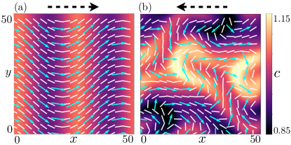
Figure 2: (a) Motile particles (here $\mathcal{V}_{0}=0.06$ and $\mbox{Er}_{a}=-3$) relax into a rightward traveling concentration wave. Cyan arrows show the direction of particle swimming, and the background color shows the particle concentration. Particles evacuate from highly bent regions and cluster away from them. See Movie 5. (b) A leftward traveling wave of greater elastic deformation, with $(\mbox{Er}_{a},\phi,\mathcal{V}_{0})=(-7,0.1,0.06)$, which moves in the opposite direction as the mean particle swimming direction (here, $\langle\theta\rangle=0$). See Movie 6.

Moment equations. Moment equations can provide insight into stability criteria and the fully nonlinear arrested state. We consider a locally aligned particle distribution $\psi(\bm{x},\bm{p},t)\approx c(\bm{x},t)\delta(\bm{p}-\bm{m})$, with first and second orientational moments $\bm{m}:=\langle\bm{p}\rangle/c=c^{-1}\int_{S^{2}}\bm{p}\psi\,d\bm{p}$ and $\bm{\mathrm{D}}=\left<\bm{p}\bm{p}\right>/c\approx\bm{m}\bm{m}$. Using Eq. (5) we find (with $D_{t}:=\partial_{t}+\bm{u}\cdot\nabla$):

$$D_{t}c+\mathcal{V}_{0}\nabla\cdot\left(c\bm{m}\right)=D\nabla^{2}c,$$ (8)

$$D_{t}(c\bm{m})+\mathcal{V}_{0}\nabla\cdot\left(c\bm{m}\bm{m}\right)$$

$$\qquad=c\left(\bm{\mathrm{I}}\bm{m}-\bm{m}\bm{m}\bm{m}\right):\left(\nabla\bm{u}+\mathcal{W}\eta^{-1}\bm{n}\bm{n}\right)$$

$$\qquad\qquad+D\nabla^{2}(c\bm{m})-2dc\bm{m},$$ (9)

$$D_{t}\bm{n}=\left(\bm{\mathrm{I}}\bm{n}-\bm{n}\bm{n}\bm{n}\right):\left(\nabla\bm{u}+\mathcal{W}\gamma^{-1}c\,\bm{m}\bm{m}\right)$$

$$\qquad\qquad+\gamma^{-1}(\bm{\mathrm{I}}-\bm{n}\bm{n})\cdot\nabla^{2}\bm{n}.$$ (10)

Motivated by Figs. 1b and 2a, we seek one-dimensional solutions. Writing $\bm{m}=(\cos\Theta,\sin\Theta)$ and $\bm{n}=(\cos\Phi,\sin\Phi)$ yields unwieldy evolution equations for $c$, $\Theta$, and $\Phi$ (see [55]), but progress is possible in various asymptotic limits. For vanishing rotational viscosity, $\gamma\rightarrow 0$, and large anchoring strength, $\mathcal{W}\gg 1$, we pursue a regular perturbation expansion $(\Phi,\Theta)=(\Phi_{0},\Theta_{0})+\mathcal{W}^{-1}(\Phi_{1},\Theta_{1})+\cdots$. At leading order we find $\Theta_{0}=\Phi_{0}$, and at first order,

$$\partial_{t}c +\mathcal{V}_{0}\left(c\cos\Theta_{0}\right)_{x}=Dc_{xx},$$ (11)

$$\partial_{t}\Theta_{0} +\mathcal{V}_{0}\partial_{x}\sin\Theta_{0}=-\mbox{Er}_{a}\phi\,c\cos^{3}\Theta_{0}\sin\Theta_{0}$$

$$\qquad+\frac{2D}{c}\partial_{x}c\partial_{x}\Theta_{0}+((\eta c)^{-1}+D)\partial_{xx}\Theta_{0}.$$ (12)

To study the first arrested state (Fig. 1b), we first consider immotile particles, $\mathcal{V}_{0}=0$. By (11), the concentration relaxes to uniformity, $c=1$, and the dynamics are governed by (12) alone. At equilibrium, denoted by $\tilde{\Theta}$, and defining $\xi=2\pi\mathcal{L}^{-1}x$,

$$\partial_{\xi\xi}\tilde{\Theta}+\mathcal{A}\cos^{3}\tilde{\Theta}\sin\tilde{\Theta}=0,$$ (13)

where we have introduced an activity parameter

$$\mathcal{A}=\frac{-\mbox{Er}_{a}\phi\mathcal{L}^{2}}{(2\pi)^{2}(D+\eta^{-1})},$$ (14)

and $\mathcal{A}>0$ for extensile particle stress.

Integration of Eq. (13) yields a closed-form representation of $\tilde{\Theta}$ in terms of $\vartheta:=\|\tilde{\Theta}\|_{\infty}$:

$$\cos\tilde{\Theta}=\frac{\cos(\vartheta)}{\sqrt{1-2\,{\rm sn}^{2}\left(B_{1}\xi;B_{2}\right)}},$$ (15)

where $B_{1}=(\mathcal{A}/8)^{1/2}\sin(2\vartheta)$ and $B_{2}=2\csc^{2}\vartheta$. Here ${\rm sn}$ is a Jacobi elliptic function, which is sinusoidal if $B_{2}=0$ and a square wave if $B_{2}=1$. The particle director line, $2\pi y/\mathcal{L}=\int_{0}^{\xi}\tan\tilde{\Theta}(s)\,ds$, for different values of $\mathcal{A}$ are plotted in Fig. 3a. Upon domain rescaling and reflection, the curve in Fig. 3a is in good quantitative agreement with the numerically observed director line in Fig. 1b ($\mathcal{A}\approx 5$).

From (15), the maximum particle orientation angle, $\vartheta$, can be shown to depend on $\mathcal{A}$ via the implicit relation,

$$\frac{2}{\pi}K\left(\frac{\sin^{2}\vartheta}{2}\right)-\sqrt{\mathcal{A}}\cos\vartheta=0.$$ (16)

Here $K(\cdot)$ is the complete elliptic integral of the first kind [55]. The only solution for $\mathcal{A}\leq 1$ is $\vartheta=0$ (see below). The value of $\vartheta$ obtained from (16) is plotted in Fig. 3b as a solid line for different values of $\mathcal{A}$, along with symbols showing values computed using full 2D simulations of the moment closure equations, showing close agreement.

Two asymptotic approximations are included in Fig. 3b, for $\mathcal{A}\approx 1$ and $\mathcal{A}\gg 1$, revealing the initial bifurcation to the first arrested state at $\mathcal{A}=1$. Only for $\mathcal{A}>1$ can a balance be reached between active and elastic stresses in a bent configuration. Although arrested solutions exist for arbitrary $\mathcal{A}$, they become unstable to transverse perturbations beyond a critical activity strength. Simulations of the moment equations (8)-(10) suggest that this transverse instability is triggered, using the same parameters as used in Fig. 1b, at $\mathcal{A}\approx 9.5$.

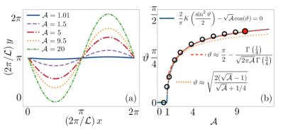
Figure 3: (a) Nearly-sinusoidal particle director line (as in Fig. 1b) for a range of activity parameters, $\mathcal{A}$. (b) The maximum orientation angle at equilibrium, $\vartheta=\|\tilde{\Theta}\|_{\infty}$, as a function of $\mathcal{A}$. Solid, dashed, and dotted lines are from numerical solution of (16), and approximations for $\mathcal{A}\gg 1$, and for $\mathcal{A}\approx 1$, respectively. Symbols are from numerical simulation of the moment equations (8)-(10). The filled symbol is a second critical $\mathcal{A}$ beyond which the 1D arrested state is unstable to transverse perturbations.

Traveling waves. We now take up the question of the periodic traveling waves observed for motile particles ($\mathcal{V}_{0}>0$), by studying (11)-(12) in a comoving frame, $\xi:=x-\omega t$, where $\omega$ is the (unknown) wave speed.

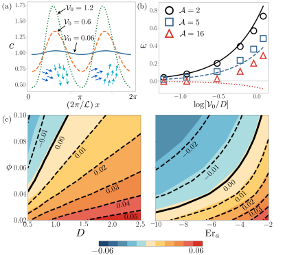
Figure 4: (a) Concentration deviations for fixed $\mathcal{A}=2$ and (dimensionless) swimming speeds $\mathcal{V}_{0}\in\{0.06,0.6,1.2\}$, with a diagram of the swimmers merging into concentration bands. (b) The dimensionless wave speed $\omega$ vs. $\log(\mathcal{V}_{0}/D)$ for $\mathcal{A}\in\{2,5,16\}$. The curves are from (20) with $\tilde{\Theta}$ found numerically from  (13), and symbols are from simulations of (8)-(10). (c) Filled contours of wave speeds from numerical simulations of (11) and (12), compared with the theoretical expression (20) (black curves) for a range of diffusivity $D$ (left) and activity $\mbox{Er}_{a}$ (right).

Using that $(c,\Theta_{0})=(1,\tilde{\Theta})$ is a periodic solution with trivial wave speed $\omega=0$ when $\mathcal{V}_{0}=0$, we seek periodic solutions with $\mathcal{V}_{0}\neq 0$ as perturbations of the $\mathcal{V}_{0}=0$ solution. A second regular perturbation expansion is thus considered, $(c,\,\Theta_{0},\,\omega)=(1,\,\Theta^{(0)},\,0)+\mathcal{V}_{0}(c^{(1)},\,\Theta^{(1)},\,\omega^{(1)})+\cdots$.

At leading order, $\Theta^{(0)}(\xi)=\tilde{\Theta}(\xi)$ as in (15). At terms of $O(\mathcal{V}_{0})$, we obtain a system of equations for $c^{(1)}$ and $\Theta^{(1)}$ in terms of $\tilde{\Theta}$:

$$\partial_{\xi\xi}c^{(1)}=\frac{1}{D}\partial_{\xi}\cos\tilde{\Theta},$$ (17)

$$\partial_{\xi\xi}\Theta^{(1)}=-\mathcal{A}\,G(\tilde{\Theta})\,\Theta^{(1)}+F(\xi),$$ (18)

where $G(\tilde{\Theta})=\cos^{4}\tilde{\Theta}-3\cos^{2}\tilde{\Theta}\sin^{2}\tilde{\Theta}$ and

$$F(\xi)=\left(\frac{2+\eta D}{1+\eta D}\right)c^{(1)}\partial_{\xi\xi}\tilde{\Theta}\\ +\frac{\eta}{2\pi(1+\eta D)}\left(\mathcal{L}(\cos\tilde{\Theta}-\omega^{(1)})-4\pi Dc^{(1)}_{\xi}\right)\partial_{\xi}\tilde{\Theta}.$$ (19)

Using the requirement of periodic boundary conditions, the wave speed to leading order in $\mathcal{V}_{0}$ is given by

$$\omega\sim(\mathcal{V}_{0}/2)\left[\left(5I_{1}-3I_{2}/I_{3}\right)+(\eta D)^{-1}\left(I_{1}-I_{2}/I_{3}\right)\right],$$ (20)

where $I_{1}=(2\pi)^{-1}\int_{0}^{2\pi}\cos\tilde{\Theta}\,d\xi$, $I_{2}=\int_{0}^{2\pi}\cos\tilde{\Theta}\tilde{\Theta}_{\xi}^{2}\,d\xi$, and $I_{3}=\int_{0}^{2\pi}\tilde{\Theta}_{\xi}^{2}\,d\xi$ (see [55]). This wavespeed is exact for the linearized equations (17)-(18), so any discrepancy from the behavior of (11)-(12) is due to linearizing about the $\mathcal{V}_{0}=0$ steady state. In terms of parameters, this error is $O(\mathcal{V}_{0}^{2}\mathcal{L}^{2}/D^{2},\mathcal{V}_{0}^{2}\mathcal{L}^{2}\mathcal{A}^{2}/D^{2})$ [55]. In particular, the linearized concentration equation (17) is valid for small $\mathcal{V}_{0}\mathcal{L}/D$, while the validity of the linearized $\Theta$ equation (18) additionally requires that $\mathcal{A}$ is not too large.

Figure 4a shows the steady state concentrations in the comoving frame. Deviations from uniformity grow with increasing particle speed, since the differential horizontal swimming component is more pronounced and the smoothing nature of diffusion is overcome. Particles moving horizontally (from regions of large bending) merge into a lane with more vertically swimming particles in regions of small LC bending.

Figure 4b shows a comparison between the analytical and computed wavespeeds across a range of ratios of (dimensionless) swimming speed to diffusion constants, for three different activity coefficients, $\mathcal{A}$. The predictions are in good agreement for small $\mathcal{V}_{0}/D$ as expected, and, for small $\mathcal{A}$, remain fairly accurate even for larger $\mathcal{V}_{0}/D$. For fixed $\mathcal{V}_{0}=0.06$, the contour plots in Fig. 4c show that the theory is accurate for larger particle volume fractions $\phi$ when $D$ is also large or $|\mbox{Er}_{a}|$ is small.

Direction reversal to retrograde wave propagation is also captured, as shown with solid curves in Figs. 4c. The concentration wave passes opposite the direction of swimmer motion for sufficiently large $\phi$, though this is counteracted by large diffusivity, $D$, or small activity, $|\mbox{Er}_{a}|$. For large $\mathcal{A}$, Fig. 4b ($\mathcal{A}=16$) indicates that the traveling wave undergoes yet another direction reversal as $\mathcal{V}_{0}/D$ is increased, so that the wave once again travels in the same direction as the active particle motion. Wave speeds for other values of $\mathcal{A}$ are included in [55].

As a final approximation, taking $\tilde{\Theta}\approx\vartheta\cos\xi$ with $\vartheta^{2}=2(\sqrt{\mathcal{A}}-1)/(\sqrt{\mathcal{A}}+1/4)\ll 1$ (see Fig. 3b), we find

$$\omega\approx\frac{9\mathcal{V}_{0}}{8\sqrt{\mathcal{A}}}.$$ (21)

This estimate is comparable to the actual values reported in Fig. 4c. The wavespeed is naturally enhanced by faster swimming, but is reduced by larger activity or particle volume fraction, since these contribute to larger LC deformations, thereby hindering particle transport.

Conclusion. We have shown that the bend instability of a suspension of active extensile particles may be tamed by elastic stresses in a surrounding anisotropic, viscoelastic fluid, leading to arrested, flowing states. The degree of LC deformation in the arrested state depends on the active Ericksen number and the active particle concentration. When the particles are motile, traveling concentration waves ensue, including a dramatic, periodic thrashing mode.

Future work is certainly needed; we did not explore the role of a number of parameters (e.g. $\lambda$). Nor did we include anisotropic viscous response, particle deformability [68], or elastic interactions between active particles through the LC, which has been considered in Refs. [69, 70], all of which may be important in some manifestations of this system. Nevertheless, the analytical descriptions of the arrested states and traveling wave speeds can provide a benchmark for examining more complex states which emerge at yet higher particle concentrations, which should be useful given the large number of parameters needed to characterize the system.

Acknowledgements. Support for this research was provided by the VCRGE with funding from the Wisconsin Alumni Research Foundation. LO acknowledges support by the NSF (DMS-2406003).

.

Arrested development and traveling waves of active suspensions
in nematic liquid crystals: Supplementary material
Jingyi Li, Laurel Ohm, and Saverio E. Spagnolie

I Equations of Motion

I.1 Swimmer distribution function

The active particles are modeled as prolate ellipsoids with major and minor axis lengths $2a$ and $2b$, and each particle thus has volume $v=4\pi ab^{2}/3$. Particles are assumed to reside inside a cubic domain with linear dimension $L$, and volume $V:=L^{3}$. The number of particles, $N$, is assumed constant, and we define the particle volume fraction as $\phi:=Nv/V$. The particle position in space is denoted by $a\bm{x}$, and its orientation by $\bm{p}\in\mathbb{S}^{2}$, the unit sphere in $\mathbb{R}^{3}$. We define the number density of active particles, $\psi^{*}(a\bm{x},\bm{p},Tt)=NL^{-3}\psi(\bm{x},\bm{p},t)$, where $T$ is a dimensional time (to be defined), and $\bm{x}\in[0,\mathcal{L}]^{3}$ and $t\geq 0$ are dimensionless, with $\mathcal{L}:=L/a$. The total number of particles in the system is given by

$$N=\int_{\mathcal{D}}\int_{\mathbb{S}^{2}}\psi^{*}(a\bm{x},\bm{p},Tt)\,d\bm{p}\,d(a\bm{x}),$$ (22)

or

$$1=\frac{1}{\mathcal{L}^{3}}\int_{\mathcal{D}}\int_{\mathbb{S}^{2}}\psi(\bm{x},\bm{p},t)\,d\bm{p}\,d\bm{x},$$ (23)

where $\mathcal{D}$ is the dimensionless fluid domain with $|\mathcal{D}|=\mathcal{L}^{3}$. For example, a uniformly concentrated, isotropic suspension has $\psi^{*}=N/L^{3}$, or $\psi=1/\mathcal{L}^{3}$. The concentration of particles is denoted by $c^{*}(a\bm{x},Tt)=NL^{-3}c(\bm{x},t)$, where

$$c(\bm{x},t)=\int_{\mathbb{S}^{2}}\psi(\bm{x},\bm{p},t)\,d\bm{p},$$ (24)

and we have

$$\frac{1}{\mathcal{L}^{3}}\int_{\mathcal{D}}c(\bm{x},t)\,d\bm{x}=1,$$ (25)

so that a uniform concentration has $c(\bm{x},t)\equiv 1$. Higher moments will also be used, in particular the first and second orientational moments, defined on the dimensionless particle distribution as

$$\langle\bm{p}\rangle:=\int_{\mathbb{S}^{2}}\bm{p}\,\psi(\bm{x},\bm{p},t)\,d\bm{p},\,\,\,\,\langle\bm{p}\bm{p}\rangle:=\int_{\mathbb{S}^{2}}\bm{p}\bm{p}\,\psi(\bm{x},\bm{p},t)\,d\bm{p},$$ (26)

respectively, with $\bm{p}\bm{p}$ a dyadic product.

We will also use normalized moments,

$$\bm{m}(\bm{x},t):=\frac{\langle\bm{p}\rangle}{c(\bm{x},t)},\,\,\,\,\bm{\mathrm{D}}(\bm{x},t):=\frac{\langle\bm{p}\bm{p}\rangle}{c(\bm{x},t)}.$$ (27)

Here $\bm{m}$ is the active polar order parameter, and $\bm{\mathrm{D}}$ relates to the nematic order parameter, $\bm{\mathrm{Q}}$, via $\bm{\mathrm{Q}}=(\bm{\mathrm{D}}-\bm{\mathrm{I}}/3)$.

Finally, we define a Dirac delta function on the dimensional spatial variables, $\delta^{*}(a\bm{x})$, defined so that

$$\int_{\mathcal{D}^{*}}\delta^{*}(a\bm{x}-a\bm{x}_{0})\,d(a\bm{x})=1,$$ (28)

for any point $a\bm{x}_{0}\in\mathcal{D}^{*}$, and a dimensionless delta function $\delta(\bm{x}-\bm{x}_{0}):=a^{3}\delta^{*}(a\bm{x}-a\bm{x}_{0})$, so that

$$\int_{\mathcal{D}}\delta(\bm{x}-\bm{x}_{0})\,d\bm{x}=1.$$ (29)

I.2 Liquid crystal dynamics

We will use an Ericksen-Leslie description of the liquid crystal (LC) [54, 9], which is assumed to be deep in the nematic phase. The local molecular orientation is denoted by $\bm{n}$. Director fields confined to two dimensions will be written in terms of a single angle $\Phi$, or $\bm{n}=(\cos{\Phi},\sin{\Phi},0)$. In the one-constant approximation, the elastic energy density is $(K/2)|\nabla^{\prime}\bm{n}|^{2}=(K/2a^{2})|\nabla\bm{n}|^{2}$, with $K$ the Frank elastic constant, $\nabla^{\prime}$ and $\nabla$ the del operators with respect to the dimensional and dimensionless positions $a\bm{x}$ and $\bm{x}$, respectively.

We now consider the effect of introducing $N$ identically shaped active particles into the LC. The $j^{th}$ active particle position is written as $a\bm{x}_{0}^{(j)}$ and its orientations as $\bm{p}^{(j)}$. The boundary conditions are assumed to be finite-strength (‘weak’) tangential anchoring conditions with anchoring strength $W$. $K$ and $W$ have units of force and force per length, respectively. We assume that the bodies are large compared to the molecular constituents of the liquid crystal, but small compared to the length over which $\bm{n}$ is varying (a Type-VI system in the language of Ref. [8]). We can then incorporate the associated moment into the volumetric energy density consistent with the Rapini-Papoular [71, 72] surface anchoring approximation. Denoting the energy density as $(K/a^{2})\mathcal{F}$, we write

$$\mathcal{F}=\frac{1}{2}|\nabla\bm{n}|^{2}+\left(\frac{a^{2}}{K}\right)\frac{SW}{2a^{3}}\sum_{j=1}^{N}\delta(\bm{x}-\bm{x}_{0}^{(j)})\left(1-(\bm{n}\cdot\bm{p}^{(j)})^{2}\right).$$ (30)

Here $S$ is the surface area of an individual particle; $S\sim\pi^{2}ab(1+O((b/a)^{2}))$ for slender, rod-like particles. If the LC and active particle directions are confined to 2D, writing $\bm{p}^{(j)}=(\cos{\theta_{j}},\sin{\theta_{j}},0)$, Eq. (30) is equivalent to

$$\mathcal{F}=\frac{1}{2}|\nabla\Phi|^{2}+\frac{\mathcal{W}}{2}\sum_{j=1}^{N}\sin^{2}(\theta_{j}-\Phi)\delta(\bm{x}-\bm{x}_{0}^{(j)}),$$ (31)

where we have introduced the dimensionless anchoring strength

$$\mathcal{W}=\frac{SW}{aK}.$$ (32)

Defining $\bm{h}:=(\bm{\mathrm{I}}-\bm{n}\bm{n})\cdot\bm{H}$, where $\bm{H}=-\delta\mathcal{F}/\delta\bm{n}$ is the (dimensionless) LC molecular field [9], we have

$$\bm{h}=(\bm{\mathrm{I}}-\bm{n}\bm{n})\cdot\left(\nabla^{2}\bm{n}+\mathcal{W}\sum_{j=1}^{N}(\bm{n}\cdot\bm{p}^{(j)})\bm{p}^{(j)}\delta(\bm{x}-\bm{x}_{0}^{(j)})\right).$$ (33)

In two dimensions, we write $\bm{h}=h\bm{n}^{\perp}$, with $\bm{n}^{\perp}=(-\sin{\Phi},\cos{\Phi},0)$, so that

$$h=\nabla^{2}\Phi+\frac{\mathcal{W}}{2}\sum_{j=1}^{N}\sin(2(\theta_{j}-\Phi))\delta(\bm{x}-\bm{x}_{0}^{(j)}).$$ (34)

Note that $h=0$ at equilibrium. For a continuum of active particles, in terms of $\psi^{*}$,

$$\bm{h}=(\bm{\mathrm{I}}-\bm{n}\bm{n})\cdot\left(\nabla^{2}\bm{n}+\mathcal{W}\int_{\mathbb{S}^{2}}\psi^{*}(\bm{x}^{*},\bm{p},t^{*})(\bm{n}\cdot\bm{p})\bm{p}\,d\bm{p}\right)=(\bm{\mathrm{I}}-\bm{n}\bm{n})\cdot\left(\nabla^{2}\bm{n}+\mathcal{W}\bm{n}\cdot\left<\bm{p}\bm{p}\right>\right).$$ (35)

In 2D, with $\bm{h}=h\bm{n}^{\perp}$, we have

$$h=\nabla^{2}\Phi+\mathcal{W}\bm{n}^{\perp}\bm{n}:\left<\bm{p}\bm{p}\right>=\nabla^{2}\Phi+\mathcal{W}\bm{n}^{\perp}\bm{n}:\left<\bm{p}\bm{p}\right>,$$ (36)

where $\bm{A}:\bm{B}=A_{ij}B_{ji}$, and we recall that $\langle\bm{p}\bm{p}\rangle$ has units of inverse volume. We write the stress corresponding to the elastic free energy as $\bm{\sigma}^{*}_{r}(a\bm{x},Tt):=(K/a^{2})\bm{\sigma}_{r}(\bm{x},t)$, where

$$\bm{\sigma}_{r}(\bm{x},t)=-\nabla\bm{n}\cdot\nabla\bm{n}^{T}-\frac{\lambda}{2}(\bm{n}\bm{h}+\bm{h}\bm{n})+\frac{1}{2}(\bm{n}\bm{h}-\bm{h}\bm{n}).$$ (37)

Here $\lambda$ is called the tumbling parameter (see Landau & Lifschitz [54, Ch. 6]).

We now move on to dynamics. At this point we are motivated select the timescale, $T=\mu a^{2}/K$, and we define the fluid velocity field $\bm{u}^{*}(a\bm{x},Tt):=K(\mu a)^{-1}\bm{u}(\bm{x},t)$, where $\mu$ is the solvent viscosity. The deviatoric viscous stress is written as $\bm{\sigma}_{v}^{*}(a\bm{x},Tt):=(K/a^{2})\bm{\sigma}_{v}(\bm{x},t)$, where

$$\bm{\sigma}_{v}(\bm{x},t)=2\mathbf{E}+\mu_{1}^{\prime}\bm{n}\bm{n}(\bm{n}\cdot\mathbf{E}\cdot\bm{n})+\mu_{2}^{\prime}(\bm{n}\mathbf{E}\cdot\bm{n}+\bm{n}\cdot\mathbf{E}\bm{n}).$$ (38)

Here $\mathbf{E}=(\nabla\bm{u}+\nabla\bm{u}^{T})/2$ is the (dimensionless) symmetric rate of strain tensor, and $\mu_{1}^{\prime}$ and $\mu_{2}^{\prime}$ are dimensionless viscosity coefficients (which we take to be zero in the main text).

The particles are assumed to generate a force dipole on the surrounding fluid. In three dimensions, each particle is assumed to generate a force $-f$ in each direction $\pm\bm{p}$, and since the particle has length $2a$, we will model the dipole strength as $\sigma_{0}=2af$. The total stress generated by the active particles in a given volume of fluid is written as $\bm{\sigma}^{*}_{a}(a\bm{x},Tt)=(K/a^{2})\bm{\sigma}_{a}(\bm{x},t)$, where (integrating by parts),

$$\nabla^{\prime}\cdot\bm{\sigma}^{*}_{a}(a\bm{x},Tt)=\int_{\mathcal{D}^{*}}\int_{\mathbb{S}^{2}}\sigma_{0}\bm{p}\bm{p}\nabla^{\prime}\delta^{*}(a\bm{x}-a\bm{x}_{0})\psi^{*}(a\bm{x}_{0},\bm{p},Tt)\,d\bm{p}\,d(a\bm{x}_{0})$$ (39)

$$=\nabla^{\prime}\cdot\int_{\mathbb{S}^{2}}\sigma_{0}\bm{p}\bm{p}\psi^{*}(a\bm{x},\bm{p},Tt)\,d\bm{p},$$ (40)

so that the dimensionless active stress is given by

$$\bm{\sigma}_{a}(\bm{x},t)=\mbox{Er}_{a}\phi\langle\bm{p}\bm{p}\rangle=\mbox{Er}_{a}\phi c\bm{\mathrm{D}}.$$ (41)

Here we have defined the active Ericksen number, which depends on the particle concentration:

$$\mbox{Er}_{a}=\frac{a^{2}\sigma_{0}}{Kv}=\frac{2f}{K}\frac{a^{3}}{v},$$ (42)

recalling that $v$ is the particle volume and $\phi$ is the particle volume fraction. With $\mbox{Er}_{a}<0$, the active particle is a ‘pusher’ particle, and with $\mbox{Er}_{a}>0$, the particle is a ‘puller’ particle.

Combining the stresses above, momentum balance and continuity are then expressed as

$$-\nabla p+\nabla\cdot\left(\bm{\sigma}_{r}+\bm{\sigma}_{v}+\mbox{Er}_{a}\phi c\bm{\mathrm{D}}\right)=\bm{0},$$ (43)

$$\nabla\cdot\bm{u}=0.$$ (44)

The Ericksen-Leslie equations are closed with a description of the director field dynamics:

$$\frac{\mbox{D}\bm{n}}{\mbox{D}t}=(\bm{\mathrm{I}}-\bm{n}\bm{n})\cdot\left(\bm{n}\cdot\nabla\bm{u}+\frac{1}{\gamma}\bm{h}\right)=(\bm{\mathrm{I}}-\bm{n}\bm{n})\cdot\left[\bm{n}\cdot\nabla\bm{u}+\frac{1}{\gamma}\left(\nabla^{2}\bm{n}+\mathcal{W}c\bm{n}\cdot\bm{\mathrm{D}}\right)\right],$$ (45)

where $\mu\gamma$ is the rotational viscosity (and $\gamma$ is dimensionless) [9].

I.3 Dynamics of the active suspension

Conservation of the total number of swimmers results in a Smoluchowski equation for $\psi$,

$$\psi_{t}+\nabla\cdot(\dot{\bm{x}}\psi)+\nabla_{\bm{p}}\cdot(\dot{\bm{p}}\psi)=0,$$ (46)

where $\nabla_{\bm{p}}=(\bm{\mathrm{I}}-\bm{p}\bm{p})\cdot(\partial/\partial\bm{p})$ and $\dot{\bm{x}}$ and $\dot{\bm{p}}$ are the (dimensionless) active particle translational and rotational velocities [61]. Let us first motivate a model for the reorientation rate of an individual active particle or swimmer in the presence of the nematic LC field. Absent a velocity field, and assuming that $\bm{n}$ remains frozen, the moment on the LC as described above is $SW(\bm{n}\cdot\bm{p})$, and the corresponding torque on the active particle is thus $-SW(\bm{n}\cdot\bm{p})$. This torque is balanced by a viscous response. As a first approximation, we thus model the response in dimensionless variables (and $\dot{\bm{p}}=d\bm{p}/dt$) as

$$\eta\dot{\bm{p}}=\left(\bm{\mathrm{I}}-\bm{p}\bm{p}\right)\cdot\left(\mathcal{W}(\bm{n}\cdot\bm{p})\bm{n}\right).$$ (47)

In a Newtonian fluid, $\eta\sim 16\pi\left(6\log(2a/b)-3\right)^{-1}$ as $b/a\to 0$ (e.g. for rod-like particles). In general this drag coefficient depends on the particle orientation relative to the director field, but at large anchoring strengths it represents only rotational drag on a nearly aligned body.

We consider a model for the (dimensionless) velocities, then, in which

$$\dot{\bm{x}}=\bm{u}+\mathcal{V}_{0}\bm{p}-D\displaystyle\frac{\nabla\psi}{\psi},$$ (48)

$$\dot{\bm{p}}=(\bm{\mathrm{I}}-\bm{p}\bm{p})\cdot\left[\bm{p}\cdot\nabla\bm{u}+\displaystyle\frac{\mathcal{W}}{\eta}(\bm{n}\cdot\bm{p})\bm{n}\right]-d\displaystyle\frac{\nabla_{\bm{p}}\psi}{\psi}.$$ (49)

With $V_{0}^{*}$, $D^{*}$, and $d^{*}$ the dimensional swimming speed, translational diffusion constant, and rotational diffusion constant, respectively, we have defined their dimensionless analogs via $V_{0}^{*}=K\mathcal{V}_{0}/\mu a$, $D^{*}=KD/\mu$, and $d^{*}=Kd/(\mu a^{2})$. These particle velocities are simple modeling choices. A force on a body in a nematic LC can also result in a transverse lift [73], which we neglect. We also neglect long-range elastic forces between the active particles, and the associated aggregation [74], under the assumption that hydrodynamic effects are dominant. Sokolov et al., studied the interactions of multiple swimming bodies [69].

I.4 Dimensionless groups and characteristic values

The dimensionless groups governing the system presented above are as follows:

$$\centering\begin{cases}\mathcal{L}=\displaystyle\frac{L}{a}&\mbox{(relative system size)}\\[8.0pt] \phi=\displaystyle\frac{Nv}{L^{3}}&\mbox{(particle volume fraction)}\\[8.0pt] \mbox{Er}_{a}=\displaystyle\frac{2f}{K}\frac{a^{3}}{v}&\mbox{(active Ericksen number)},\\[8.0pt] \mathcal{W}=\displaystyle\frac{SW}{aK}&\mbox{(LC anchoring strength)},\\[8.0pt] \mathcal{V}_{0}=\displaystyle\frac{\mu aV_{0}^{*}}{K}&\mbox{(relative swimming speed)},\\[8.0pt] \eta&\mbox{(rotational drag coefficient)},\\[8.0pt] D=\displaystyle\frac{\mu D^{*}}{K}&\mbox{(translational diffusivity)},\\[8.0pt] d=\displaystyle\frac{\mu a^{2}d^{*}}{K}&\mbox{(rotational diffusivity)},\\[8.0pt] \gamma=\displaystyle\frac{\gamma^{*}}{\mu}&\mbox{(LC rotational viscosity)},\\[8.0pt] \lambda&\mbox{(LC tumbling parameter)}.\end{cases}\@add@centering$$

Characteristic values for the dimensional parameters above may be estimated using B. subtilis cells in DSCG, a lyotropic chromonic phase [62]. We have approximately: $a=3\mu$m, $b=0.5\mu$m, $S=15\mu$m², $\eta\approx 4$, $V_{0}^{*}=20\mu$m/s (in water), from which we estimate $f\approx 6\pi\mu a\mathcal{V}_{0}=6\pi(10^{-2}\mbox{dyn s/cm}^{2})(3\mu\mbox{m})(20\mu\mbox{m/s})=10^{-7}$dyn, $v=4\pi ab^{2}/3=3.1\mu$m³, $K=10^{-7}-10^{-6}$dyn, $W\approx 10^{-8}-10^{-7}$dyn/$\mu$m, and $\gamma^{*}=10^{-6}-10^{-4}$dyn s/cm². For the diffusion constants, by the Stokes-Einstein relation, using $k_{b}T=4.11\cdot 10^{-21}\mbox{J}=4.11\cdot 10^{-14}$dyn cm, we have $D^{*}\approx k_{b}T/(6\pi\mu a)=10^{-9}$cm²/s and $d^{*}\approx k_{b}T/(8\pi\mu a^{3})=0.01$s^-1.

Assuming a domain with dimensions $\mathcal{L}=L/a=50$, the above values produce the following estimates of the dimensionless parameters:

$$\centering\begin{cases}|\mbox{Er}_{a}|\approx 1-20,\\ \mathcal{W}\approx 0.5-5,\\ \mathcal{V}_{0}\approx 0.006-0.06,\\ \eta\approx 4,\\ D\approx 10^{-5}-10^{-4},\\ d\approx 10^{-5}-10^{-4},\\ \gamma\approx 10^{-4},\end{cases}\@add@centering$$ (50)

and we set $\lambda=1$. These parameter values motivate the values used in the main text. Volume fractions in experiments range from dilute to non-dilute; in the paper we commonly take $\phi\approx 0.02$ unless otherwise stated.

II Moment equations and limits

II.1 One direction dependence, strong anchoring strength, small rotational viscosity

For a locally aligned particle distribution $\psi(\bm{x},\bm{p},t)=c(\bm{x},t)\delta(\bm{p}-\bm{m})$, where $\bm{m}$ is the active polar order parameter (27), instead of evolving the full system (43)-(46), we seek to approximate the active particle dynamics using a system of moment equations, as given in the main text. For convenience, we rewrite the system here alongside the fluid equations:

$$\frac{\mbox{D}c}{\mbox{D}t}+\nabla\cdot\left[\mathcal{V}_{0}(c\bm{m})\right]=D\nabla^{2}c,$$ (51)

$$\frac{\mbox{D}(c\bm{m})}{\mbox{D}t}+\nabla\cdot\left[\mathcal{V}_{0}(c\bm{m}\bm{m})\right]=\left[c\bm{\mathrm{I}}\bm{m}-c\bm{m}\bm{m}\bm{m}\right]:\left[\nabla\bm{u}+\frac{\mathcal{W}}{\eta}\bm{n}\bm{n}\right]+D\nabla^{2}(c\bm{m})-2dc\bm{m},$$ (52)

$$\frac{\mbox{D}\bm{n}}{\mbox{D}t}=\left[\bm{\mathrm{I}}\bm{n}-\bm{n}\bm{n}\bm{n}\right]:\left[\nabla\bm{u}+\frac{\mathcal{W}}{\gamma}(c\bm{m}\bm{m})\right]+\frac{1}{\gamma}(\bm{\mathrm{I}}-\bm{n}\bm{n})\cdot\nabla^{2}\bm{n},$$ (53)

$$-\nabla p+\nabla^{2}\bm{u}+\nabla\cdot\left(\bm{\sigma}_{r}+\mbox{Er}_{a}\phi(c\bm{m}\bm{m})\right)=\bm{0},$$ (54)

$$\nabla\cdot\bm{u}=0.$$ (55)

We now seek solutions to (51)-(55) which depend only on the horizontal variable, $x$. Writing $c=c(x,t)$, $\bm{m}=(\cos{\Theta(x,t)},\sin{\Theta(x,t)},0)$, $\bm{n}=(\cos{\Phi(x,t)},\sin{\Phi(x,t)},0)$ and $\bm{u}=(0,v(x,t),0)$, Eqs. (51), (52) and (53) reduce to:

$$c_{t}+\mathcal{V}_{0}\left(\cos(\Theta)c_{x}-\sin(\Theta)\Theta_{x}c\right)=Dc_{xx},$$ (56)

$$\Theta_{t}+\mathcal{V}_{0}\cos(\Theta)\Theta_{x}=\cos^{2}(\Theta)v_{x}-\frac{\mathcal{W}}{2\eta}\sin[2(\Theta-\Phi)]+D\left(\Theta_{xx}+\frac{2c_{x}}{c}\Theta_{x}\right),$$ (57)

$$\Phi_{t}=\cos^{2}(\Phi)v_{x}+\frac{\mathcal{W}c}{2\gamma}\sin[2(\Theta-\Phi)]+\frac{1}{\gamma}\Phi_{xx}.$$ (58)

Solving for $v_{x}$ using Eq. (54), we have

$$-p_{x}+\partial_{x}\left[-(\Phi_{x})^{2}+\frac{\lambda}{2}\left(\Phi_{xx}+\frac{\mathcal{W}c}{2}\sin[2(\Theta-\Phi)]\right)\sin(2\Phi)+\mbox{Er}_{a}\phi c\cos^{2}{\Theta}\right]=0,$$ (59)

$$v_{xx}+\partial_{x}\left[(1-\lambda\cos(2\Phi))\left(\frac{1}{2}\Phi_{xx}+\frac{\mathcal{W}c}{4}\sin[2(\Theta-\Phi)]\right)+\frac{\mbox{Er}_{a}\phi c}{2}\sin{2\Theta}\right]=0.$$ (60)

Therefore, using periodicity in $x$, the fluid velocity and pressure satisfy

$$p(x)=-(\Phi_{x})^{2}+\frac{\lambda}{2}\left(\Phi_{xx}+\frac{\mathcal{W}c}{2}\sin[2(\Theta-\Phi)]\right)\sin(2\Phi)+\mbox{Er}_{a}\phi c\cos^{2}{\Theta},$$ (61)

$$v_{x}=(\lambda\cos(2\Phi)-1)\left(\frac{1}{2}\Phi_{xx}+\frac{\mathcal{W}c}{4}\sin[2(\Theta-\Phi)]\right)-\frac{\mbox{Er}_{a}\phi c}{2}\sin{2\Theta}.$$ (62)

For large anchoring strength, $\mathcal{W}\gg 1$, we pursue a regular perturbation expansion,

$$\Phi=\Phi_{0}(x,t)+\mathcal{W}^{-1}\Phi_{1}(x,t)+\mathcal{W}^{-2}\Phi_{2}(x,t)+\cdots,$$ (63)

$$\Theta=\Theta_{0}(x,t)+\mathcal{W}^{-1}\Theta_{1}(x,t)+\mathcal{W}^{-2}\Theta_{2}(x,t)+\cdots.$$ (64)

At leading order, unsurprisingly, from Eq. (57) we find $\Phi_{0}=\Theta_{0}$. Inserting this relation into the velocity gradient and expanding, we find that to leading order,

$$v_{x}=-\frac{\mbox{Er}_{a}\phi c}{2}\sin(2\Theta_{0})+\frac{1}{2}(\lambda\cos(2\Theta_{0})-1)\left(\partial_{xx}\Theta_{0}+c(\Theta_{1}-\Phi_{1})\right)+O\left(\frac{1}{\mathcal{W}}\right).$$ (65)

Eq. (57) then provides an equation for the dynamics of $\Theta_{0}$ (or equivalently for $\Phi_{0}$) which, through the velocity field, depends on the difference of the active and passive fields at the next order:

$$\partial_{t}\Theta_{0}+\mathcal{V}_{0}\cos(\Theta_{0})\partial_{x}\Theta_{0}=-\mbox{Er}_{a}\phi c\cos^{3}\Theta_{0}\sin\Theta_{0}+\left(c\,g(\Theta_{0})-\frac{1}{\eta}\right)(\Theta_{1}-\Phi_{1})+(g(\Theta_{0})+D)\partial_{xx}\Theta_{0}+\frac{2Dc_{x}}{c}\partial_{x}\Theta_{0},$$ (66)

where

$$g(\Theta_{0})=\frac{1}{2}\cos^{2}(\Theta_{0})\left(\lambda\cos(2\Theta_{0})-1\right).$$ (67)

However, from Eq. (58) (replacing $\Phi_{0}$ with $\Theta_{0}$), we also have that

$$\partial_{t}\Theta_{0}=-\mbox{Er}_{a}\phi c\cos^{3}\Theta_{0}\sin\Theta_{0}+\left(g(\Theta_{0})+\frac{1}{\gamma}\right)\left[c(\Theta_{1}-\Phi_{1})+\partial_{xx}\Theta_{0}\right].$$ (68)

Combining Eqs. (66) and (68), we find

$$\Phi_{1}(x)-\Theta_{1}(x)=\frac{1}{c(c+\gamma/\eta)}\left(\gamma(\mathcal{V}_{0}c\cos(\Theta_{0})-2Dc_{x})\partial_{x}\Theta_{0}+(1-\gamma D)c\,\partial_{xx}\Theta_{0}\right).$$ (69)

In particular, we may obtain an equation for $\partial_{t}\Theta_{0}$ depending only on $\Theta_{0}$ and $c$:

$$\partial_{t}\Theta_{0}=-\mbox{Er}_{a}\phi c\cos^{3}\Theta_{0}\sin\Theta_{0}+\frac{g(\Theta_{0})+\gamma^{-1}}{1+c\eta\gamma^{-1}}\left(-\eta(\mathcal{V}_{0}c\cos(\Theta_{0})-2Dc_{x})\partial_{x}\Theta_{0}+(1+\eta Dc)\partial_{xx}\Theta_{0}\right).$$ (70)

We consider (70) in the limit of small dimensionless rotational viscosity, $\gamma\to 0$, which yields

$$\partial_{t}\Theta_{0}=-\mbox{Er}_{a}\phi c\cos^{3}\Theta_{0}\sin\Theta_{0}-\left(\mathcal{V}_{0}\cos(\Theta_{0})-2D\frac{c_{x}}{c}\right)\partial_{x}\Theta_{0}+\left(\frac{1}{\eta c}+D\right)\partial_{xx}\Theta_{0}.$$ (71)

Coupling with Eq. (56), we obtain the expressions in the main text.

II.2 No swimming: steady state analysis

We first define a scaled length $\xi=2\pi x/\mathcal{L}$, with $\xi\in[0,2\pi]$, so that, e.g., $\partial_{x}\Theta_{0}=2\pi\mathcal{L}^{-1}\partial_{\xi}\Theta_{0}$. In the absence of particle motility, the particle concentration $c$ and angle $\Theta_{0}$ satisfy Eqs. (56) and (71) with $\mathcal{V}_{0}=0$. At equilibrium, the particle concentration is $\tilde{c}\equiv 1$, while the equilibrium angle $\tilde{\Theta}$ satisfies

$$\partial_{\xi\xi}\tilde{\Theta}+\mathcal{A}\cos^{3}\tilde{\Theta}\sin\tilde{\Theta}=0.$$ (72)

Here we have defined an activity parameter

$$\mathcal{A}=\frac{-\phi\mbox{Er}_{a}\mathcal{L}^{2}}{(2\pi)^{2}(D+\eta^{-1})}$$ (73)

which incorporates not only the competition between active and passive elastic stresses (and particle volume fraction) represented by $\mbox{Er}_{a}$, but also reduces the effective activity due to diffusivity - an active Péclet number. Note that $\mathcal{A}>0$ for extensile stresses.

Multiplying by $\tilde{\Theta}_{\xi}$ and integrating yields

$$\frac{1}{2}\tilde{\Theta}_{\xi}^{2}-\frac{\mathcal{A}}{4}\cos^{4}(\tilde{\Theta})=C$$ (74)

for some constant $C$. Choosing $\tilde{\Theta}(0)=\|\tilde{\Theta}\|_{\infty}:=\vartheta$ and $\tilde{\Theta}_{\xi}(0)=0$ (which we may do without loss of generality, by phase invariance), $C$ may be written in terms of $\vartheta$, yielding

$$\tilde{\Theta}_{\xi}^{2}=\frac{\mathcal{A}}{2}\left(\cos^{4}\tilde{\Theta}-\cos^{4}\vartheta\right).$$ (75)

We will focus on extensile particles, $\mathcal{A}>0$. On the quarter domain $\xi\in[0,\pi/2$] we have $0\leq\tilde{\Theta}(\xi)\leq\vartheta$, and we may choose without loss of generality that $\tilde{\Theta}_{\xi}<0$ and $\tilde{\Theta}(\pi/2)=0$ at the boundary. This selects the appropriate branch of the square root:

$$\tilde{\Theta}_{\xi}=-\sqrt{\frac{\mathcal{A}}{2}}\sqrt{\cos^{4}\tilde{\Theta}-\cos^{4}\vartheta}.$$ (76)

The equation (76) is separable. The trivial solution, $\tilde{\Theta}=0$ and $\vartheta=0$, is always one solution. To find other solutions, we can integrate as follows:

$$\int_{\vartheta}^{\tilde{\Theta}}\frac{d\tilde{\Theta}}{\sqrt{\cos^{4}\tilde{\Theta}-\cos^{4}\vartheta}}=-\sqrt{\frac{\mathcal{A}}{2}}\xi.$$ (77)

The above integral yields a closed-form representation of $\tilde{\Theta}$ in terms of the initial angle $\vartheta=\tilde{\Theta}(0)$:

$$\tilde{\Theta}=\cos^{-1}\left(\frac{\cos(\vartheta)}{\sqrt{1-2\,{\rm sn}^{2}\left(\sqrt{\frac{\mathcal{A}}{8}}\sin(2\vartheta)\xi;2\csc^{2}(\vartheta)\right)}}\right),$$ (78)

where sn is a Jacobi elliptic sine function.

The boundary condition $\tilde{\Theta}(\pi/2)=0$ then reveals an equation for $\vartheta$:

$$\frac{-F(\vartheta)}{\cos^{2}\vartheta}=-\frac{\pi}{2}\sqrt{\frac{\mathcal{A}}{2}},$$ (79)

where

$$F(\vartheta)=\int_{0}^{\vartheta}\frac{d\Theta}{\sqrt{\frac{\cos^{4}\Theta}{\cos^{4}\vartheta}-1}}=\frac{\cos\vartheta}{\sqrt{2}}K\left(\frac{\sin^{2}\vartheta}{2}\right).$$ (80)

Here $K(\cdot)$ is the complete elliptic integral of the first kind:

$$K\left(z\right)=\int_{0}^{\pi/2}\frac{dt}{\sqrt{1-z\cos^{2}t}}.$$ (81)

The initial angle $\vartheta$ is thus selected by the solution to

$$\frac{2}{\pi}K\left(\frac{\sin^{2}\vartheta}{2}\right)-\sqrt{\mathcal{A}}\cos\vartheta=0.$$ (82)

This is a monotonically increasing function of $\vartheta$, so the potential for a root is determined by checking the function value as $\vartheta\to 0$. Since $K(z)\to\pi/2$ as $z\to 0$, the critical value of $\mathcal{A}$ for which a non-trivial solution appears is $\mathcal{A}=1$. Solutions begin to emerge when $\mathcal{A}\geq 1$, increasing continuously from $\vartheta=0$. For values of $\mathcal{A}$ just larger than 1, expanding around small $\vartheta=0$ to second order, we find

$$\vartheta\approx\sqrt{\frac{2(\sqrt{\mathcal{A}}-1)}{\sqrt{\mathcal{A}}+1/4}}.$$ (83)

Expanding instead around $\vartheta=\pi/2$, we find

$$\vartheta\approx\frac{\pi}{2}-\frac{\Gamma\left(\frac{1}{4}\right)}{\sqrt{2\pi\mathcal{A}}\,\Gamma\left(\frac{3}{4}\right)}\approx\frac{\pi}{2}-\frac{1.18}{\sqrt{\mathcal{A}}}.$$ (84)

We may compare the approximations (83) and (84) of $\vartheta(\mathcal{A})$ to the full numerical solution of Eq. (82). These two approximations as well as the numerical solution are plotted across a range of $\mathcal{A}>0$ in Fig. 3b in the main text. Plots of the integral curves, $(2\pi y/\mathcal{L})=\int_{0}^{\xi}\tan\tilde{\Theta}(s)\,ds$, or director lines, are shown in Fig. 3a of the main text.

The secondary instability presented in Fig. 1c in the main text is a fully 2D configuration which cannot be captured by the 1D system. However, heuristically, this secondary instability may occur when the vertical extent of end-to-end aligned particles admits an unstable wavelength. For a given $\mathcal{A}$, the smallest unstable wavelength is determined by a rescaling of space with $\sqrt{\mathcal{A}}$: since $\mathcal{A}=1$ is the critical value for $x\in[0,2\pi]$, the critical smallest amplitude $\tilde{A}$ for instability is $2\tilde{A}=2\pi/\sqrt{\mathcal{A}}$. The amplitude $\tilde{A}$ may be approximated using the integral curves plotted in Fig. 3a of the main text as $\tilde{A}=\int_{0}^{\pi/2}\tan\tilde{\Theta}(s)\,ds$. Solving $\int_{0}^{\pi/2}\tan\tilde{\Theta}(s)\,ds=\pi/\sqrt{\mathcal{A}}$ for $\mathcal{A}$, we find a critical value of $\mathcal{A}\approx 4.3$.

III Dynamics of motile particles: traveling wave solutions

We now return to the moment equations, this time with $\mathcal{V}_{0}>0$. We have

$$\partial_{t}c=-\mathcal{V}_{0}\left(\cos(\Theta_{0})c\right)_{x}+Dc_{xx},$$ (85)

$$\partial_{t}\Theta_{0}=-\mbox{Er}_{a}\phi c\cos^{3}\Theta_{0}\sin\Theta_{0}-\left(\mathcal{V}_{0}\cos\Theta_{0}-2D\frac{c_{x}}{c}\right)\partial_{x}\Theta_{0}+\left(\frac{1}{\eta c}+D\right)\partial_{xx}\Theta_{0}.$$ (86)

We seek a traveling wave solution in terms of the comoving variable $\xi=2\pi\mathcal{L}^{-1}(x-\omega t)$, where the wave speed $\omega$ is to be determined. The system (85)-(86) can be rewritten in terms of $\xi$ as

$$-\omega c_{\xi}=-\mathcal{V}_{0}\left(\cos(\Theta_{0})c\right)_{\xi}+2\pi\mathcal{L}^{-1}Dc_{\xi\xi},$$ (87)

$$-\omega\partial_{\xi}\Theta_{0}=-\frac{\mbox{Er}_{a}\phi c\mathcal{L}}{2\pi}\cos^{3}\Theta_{0}\sin\Theta_{0}-\left(\mathcal{V}_{0}\cos(\Theta_{0})-4\pi\mathcal{L}^{-1}D\frac{c_{\xi}}{c}\right)\partial_{\xi}\Theta_{0}+2\pi\mathcal{L}^{-1}\left(\frac{1}{\eta c}+D\right)\partial_{\xi\xi}\Theta_{0}.$$ (88)

When $\mathcal{V}_{0}=0$, we know that Eqs. (87)-(88) admit a (trivial) traveling wave solution, namely, the stationary solution $\tilde{\Theta}$ with wave speed $\omega=0$. We thus look for nearby traveling wave solutions with $\mathcal{V}_{0}>0$. For small $\mathcal{V}_{0}$, we pursue a regular perturbation expansion $c=1+\mathcal{V}_{0}c^{(1)}(\xi)+\mathcal{V}_{0}^{2}c^{(2)}(\xi)+\cdots$, $\Theta_{0}=\Theta^{(0)}(\xi)+\mathcal{V}_{0}\Theta^{(1)}(\xi)+\mathcal{V}_{0}^{2}\Theta^{(2)}(\xi)+\cdots$, and $\omega=\mathcal{V}_{0}\omega^{(1)}+\mathcal{V}_{0}^{2}\omega^{(2)}+\cdots$. At leading order, we have

$$\partial_{\xi\xi}\Theta^{(0)}=-\mathcal{A}\cos^{3}\Theta^{(0)}\sin\Theta^{(0)},$$ (89)

with the activity parameter $\mathcal{A}$ defined in the previous section. In particular, $\Theta^{(0)}=\tilde{\Theta}$ is the steady solution found for $\mathcal{V}_{0}=0$. At $O(\mathcal{V}_{0})$, we obtain the system

$$\partial_{\xi\xi}c^{(1)}=\frac{\mathcal{L}}{2\pi D}\partial_{\xi}\cos\tilde{\Theta},$$ (90)

$$\partial_{\xi\xi}\Theta^{(1)}=-\mathcal{A}\left(\cos^{4}\tilde{\Theta}-3\cos^{2}\tilde{\Theta}\sin^{2}\tilde{\Theta}\right)\Theta^{(1)}+F(\xi),$$ (91)

where

$$F(\xi)=\left(\frac{2+\eta D}{1+\eta D}\right)c^{(1)}\partial_{\xi\xi}\tilde{\Theta}+\frac{\eta}{2\pi(1+\eta D)}\left(\mathcal{L}(\cos\tilde{\Theta}-\omega^{(1)})-4\pi Dc^{(1)}_{\xi}\right)\partial_{\xi}\tilde{\Theta}.$$ (92)

Noting that $c^{(1)}$ does not depend on $\Theta^{(1)}$, we may immediately integrate (90) to obtain

$$c^{(1)}=\frac{\mathcal{L}}{2\pi D}\int_{0}^{\xi}\cos\tilde{\Theta}(s)\,ds+k_{1}\xi+k_{2},$$ (93)

$$k_{1}=-\frac{\mathcal{L}}{(2\pi)^{2}D}\int_{0}^{2\pi}\cos\tilde{\Theta}(s)\,ds,\quad k_{2}=\pi k_{1}+\frac{\mathcal{L}}{(2\pi)^{2}D}\int_{0}^{2\pi}s\cos\tilde{\Theta}(s)\,ds,$$ (94)

where $k_{1}$ and $k_{2}$ are determined, respectively, by requiring that $c^{(1)}_{\xi}$ is periodic and $c^{(1)}$ is mean zero.

Since $c^{(1)}(\xi)$ may be determined explicitly in terms of $\tilde{\Theta}$, the term $F(\xi)$ in Eq. (91) may be considered as an inhomogeneous forcing term. We may then solve the ODE (91) explicitly using variation of parameters. We first note that $\tilde{\Theta}_{\xi}$ is a solution to the homogeneous version of (91) ($F=0$), which can be seen as follows. Using that $\tilde{\Theta}_{\xi\xi}=-\mathcal{A}\cos^{3}\tilde{\Theta}\sin\tilde{\Theta}$, we have

$$-\mathcal{A}\left(\cos^{4}\tilde{\Theta}-3\cos^{2}\tilde{\Theta}\sin^{2}\tilde{\Theta}\right)\tilde{\Theta}_{\xi} =-\mathcal{A}\partial_{\tilde{\Theta}}\left(\cos^{3}\tilde{\Theta}\sin\tilde{\Theta}\right)\tilde{\Theta}_{\xi}$$ (95)

$$=-\mathcal{A}\partial_{\xi}\left(\cos^{3}\tilde{\Theta}\sin\tilde{\Theta}\right)$$

$$=\partial_{\xi\xi\xi}\tilde{\Theta}.$$

Since we know one solution $\tilde{\Theta}_{\xi}$ of the homogeneous second order ODE, we can determine the other solution $Y$ using the Wronskian

$$W_{r}(\xi)=\tilde{\Theta}_{\xi}Y_{\xi}-\tilde{\Theta}_{\xi\xi}Y.$$ (96)

In particular, we see that $(W_{r})_{\xi}=0$, so $W_{r}$ is a constant which we may take to be 1. Then $Y$ satisfies the ODE

$$Y_{\xi}-\frac{\tilde{\Theta}_{\xi\xi}}{\tilde{\Theta}_{\xi}}Y=\frac{1}{\tilde{\Theta}_{\xi}},$$ (97)

which can be solved exactly to yield

$$Y(\xi)=\tilde{\Theta}_{\xi}\int_{0}^{\xi}\tilde{\Theta}_{\xi}^{-2}(s)\,ds.$$ (98)

Note that $Y(\xi)$ is not $2\pi$-periodic. The general solution to the homogeneous version of Eq. (91) is then given by

$$S(\xi)=C_{a}\tilde{\Theta}_{\xi}(\xi)+C_{b}Y(\xi)$$ (99)

where $C_{a}$ and $C_{b}$ are constants.

Using variation of parameters, the solution to the inhomogeneous version of Eq. (91) with $F$ as in (92) is given by

$$\Theta^{(1)}(\xi)=G_{1}(\xi)\tilde{\Theta}_{\xi}(\xi)+G_{2}(\xi)Y(\xi),$$ (100)

$$G_{1}(\xi)=G_{1}(0)-\int_{0}^{\xi}Y(s)F(s)\,ds,\quad G_{2}(\xi)=G_{2}(0)+\int_{0}^{\xi}\tilde{\Theta}_{\xi}(s)F(s)\,ds,$$ (101)

where $(G_{1})_{\xi}\tilde{\Theta}_{\xi}+(G_{2})_{\xi}Y(\xi)=0$. Note that $\Theta^{(1)}_{\xi}=G_{1}(\xi)\tilde{\Theta}_{\xi\xi}(\xi)+G_{2}(\xi)Y_{\xi}(\xi)$. To enforce periodic boundary conditions for $\Theta^{(1)}$, i.e. $\Theta^{(1)}(0)=\Theta^{(1)}(2\pi),\ \Theta^{(1)}_{\xi}(0)=\Theta^{(1)}_{\xi}(2\pi)$, we require

$$\begin{cases}G_{1}(0)\tilde{\Theta}_{\xi}(0)+G_{2}(0)Y(0)=G_{1}(2\pi)\tilde{\Theta}_{\xi}(2\pi)+G_{2}(2\pi)Y(2\pi),\\ G_{1}(0)\tilde{\Theta}_{\xi\xi}(0)+G_{2}(0)Y_{\xi}(0)=G_{1}(2\pi)\tilde{\Theta}_{\xi\xi}(2\pi)+G_{2}(2\pi)Y_{\xi}(2\pi).\end{cases}$$ (102)

Since $\tilde{\Theta}$ is periodic on $[0,2\pi]$, these conditions simplify to

$$\begin{cases}G_{2}(0)(Y(0)-Y(2\pi))=(G_{1}(2\pi)-G_{1}(0))\tilde{\Theta}_{\xi}(2\pi)+(G_{2}(2\pi)-G_{2}(0))Y(2\pi),\\ G_{2}(0)(Y_{\xi}(0)-Y_{\xi}(2\pi))=(G_{1}(2\pi)-G_{1}(0))\tilde{\Theta}_{\xi\xi}(2\pi)+(G_{2}(2\pi)-G_{2}(0))Y_{\xi}(2\pi).\end{cases}$$ (103)

By solving for $G_{2}(0)$, we may further simplify the conditions (103) to the single equation

$$(Y_{\xi}(0)-Y_{\xi}(2\pi))\left[(G_{1}(2\pi)-G_{1}(0))\tilde{\Theta}_{\xi}(2\pi)+(G_{2}(2\pi)-G_{2}(0))Y(2\pi)\right]$$ (104)

$$=(Y(0)-Y(2\pi))\left[(G_{1}(2\pi)-G_{1}(0))\tilde{\Theta}_{\xi\xi}(2\pi)+(G_{2}(2\pi)-G_{2}(0))Y_{\xi}(2\pi)\right].$$

Using the Wronskian identity $W_{r}(\xi)=\tilde{\Theta}_{\xi}Y_{\xi}-\tilde{\Theta}_{\xi\xi}Y=1$ for each $\xi$, along with the periodicity of $\tilde{\Theta}$, Eq. (104) may be simplified to the condition

$$(G_{2}(2\pi)-G_{2}(0))(Y_{\xi}(0)Y(2\pi)-Y_{\xi}(2\pi)Y(0))=0.$$ (105)

Since $Y(\xi)$ is not periodic, in order to enforce periodicity for $\Theta^{(1)}$, we need to require

$$G_{2}(2\pi)-G_{2}(0)=\int_{0}^{2\pi}\tilde{\Theta}_{\xi}F\,d\xi=0.$$ (106)

Inserting (92) into (106), we require

$$0 =\int_{0}^{2\pi}\tilde{\Theta}_{\xi}F\,d\xi=\int_{0}^{2\pi}\left(\frac{2+\eta D}{1+\eta D}\right)c^{(1)}\tilde{\Theta}_{\xi\xi}\tilde{\Theta}_{\xi}+\frac{\eta}{2\pi(1+\eta D)}\left(\mathcal{L}(\cos\tilde{\Theta}-\omega^{(1)})-4\pi Dc^{(1)}_{\xi}\right)\tilde{\Theta}_{\xi}^{2}\,d\xi,$$ (107)

or, rearranging,

$$\omega^{(1)}\int_{0}^{2\pi}\tilde{\Theta}_{\xi}^{2}\,d\xi =\int_{0}^{2\pi}\left(\cos\tilde{\Theta}-\frac{4\pi D}{\mathcal{L}}c^{(1)}_{\xi}\right)\tilde{\Theta}_{\xi}^{2}\,d\xi+\frac{2\pi(2+\eta D)}{\eta\mathcal{L}}\int_{0}^{2\pi}c^{(1)}\tilde{\Theta}_{\xi\xi}\tilde{\Theta}_{\xi}\,d\xi$$ (108)

$$=\int_{0}^{2\pi}\left(\cos\tilde{\Theta}-\frac{4\pi D}{\mathcal{L}}c^{(1)}_{\xi}\right)\tilde{\Theta}_{\xi}^{2}\,d\xi-\frac{\pi(2+\eta D)}{\eta\mathcal{L}}\int_{0}^{2\pi}c_{\xi}^{(1)}\tilde{\Theta}_{\xi}^{2}\,d\xi$$

$$=\int_{0}^{2\pi}\cos\tilde{\Theta}\tilde{\Theta}_{\xi}^{2}\,d\xi-\frac{\pi(2+5\eta D)}{\eta\mathcal{L}}\int_{0}^{2\pi}c_{\xi}^{(1)}\tilde{\Theta}_{\xi}^{2}\,d\xi.$$

Using the expression (93) for $c^{(1)}_{\xi}$, we obtain

$$\omega^{(1)}\int_{0}^{2\pi}\tilde{\Theta}_{\xi}^{2}\,d\xi =\int_{0}^{2\pi}\cos(\tilde{\Theta})\tilde{\Theta}_{\xi}^{2}\,d\xi-\frac{2+5\eta D}{2\eta D}\int_{0}^{2\pi}\left(\cos(\tilde{\Theta})+\frac{2\pi D}{\mathcal{L}}k_{1}\right)\tilde{\Theta}_{\xi}^{2}\,d\xi$$ (109)

$$=\frac{1}{2}(5I_{1}I_{3}-3I_{2})+\frac{1}{\eta D}\left(I_{1}I_{3}-I_{2}\right),$$ (110)

where we have defined

$$I_{1}=\frac{1}{2\pi}\int_{0}^{2\pi}\cos\tilde{\Theta}\,d\xi,\,\,\,\,I_{2}=\int_{0}^{2\pi}\cos\tilde{\Theta}\tilde{\Theta}_{\xi}^{2}\,d\xi,\,\,\,\,I_{3}=\int_{0}^{2\pi}\tilde{\Theta}_{\xi}^{2}\,d\xi.$$ (111)

Thus for small $\mathcal{V}_{0}$, with $\mathcal{V}_{0}>0$, the traveling wave speed is given to leading order by $\mathcal{V}_{0}\omega^{(1)}$ where

$$\omega^{(1)}=\frac{1}{2}\left(5I_{1}-3\frac{I_{2}}{I_{3}}\right)+\frac{1}{\eta D}\left(I_{1}-\frac{I_{2}}{I_{3}}\right).$$ (112)

The expression (112) is exact for the linearized equations (90)-(91), so any discrepancy from the behavior of equations (87) and (88) is due to linearizing about the $\mathcal{V}_{0}=0$ steady state. This error is $O(|\mathcal{V}_{0}c^{(1)}|^{2},|\mathcal{V}_{0}\Theta^{(1)}|^{2})$. Immediately from the expression (93) for $c^{(1)}$, we see that $|c^{(1)}|\sim\mathcal{L}D^{-1}$.

For $|\Theta^{(1)}|$, we first note that $\tilde{\Theta}_{\xi}\sim\sqrt{\mathcal{A}}$, by Eq. (76), while $\tilde{\Theta}_{\xi\xi}\sim\mathcal{A}$, by Eq. (89). Using the scalings $c^{(1)}\sim\mathcal{L}D^{-1}$ and $\omega^{(1)}\sim\sqrt{\mathcal{A}}^{-1}$, we have that the forcing term $F$ from Eq. (92) roughly satisfies $F\sim\sqrt{\mathcal{A}}\mathcal{L}\eta(1+\eta D)^{-1}+\mathcal{A}\mathcal{L}D^{-1}\lesssim\mathcal{A}\mathcal{L}D^{-1}$ for $\mathcal{A}\geq 1$. From the form (100) of $\Theta^{(1)}$, we then have $|\Theta^{(1)}|\sim\mathcal{A}\mathcal{L}D^{-1}$. The error of the linearized traveling wave speed $\mathcal{V}_{0}\omega^{(1)}$ is thus $O(\mathcal{V}_{0}^{2}\mathcal{L}^{2}/D^{2},\mathcal{V}_{0}^{2}\mathcal{L}^{2}\mathcal{A}^{2}/D^{2})$. The dependence of the error on $D$ and $\mathcal{A}=-\phi\mbox{Er}_{a}\mathcal{L}^{2}[(2\pi)^{2}(D+\eta^{-1})]^{-1}$ can be noted in Figs. 5, 6, and 7.

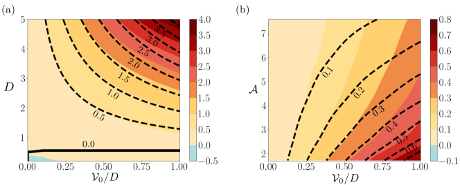
Figure 5: Contour plots of the wave speed $\omega$, computed using the reduced 1D system (56) and (70), for (a) $D\in[0.1,5]$ and $\mathcal{V}_{0}/D\in[0,1]$; (b) $\mathcal{A}\in[1.7,7.6]$ and $\mathcal{V}_{0}/D\in[0,1]$; with fixed $\gamma=0.001,\ \phi_{s}=0.04$. Dashed lines are the analytical values of $\omega^{(1)}$ given by Eq. (112).

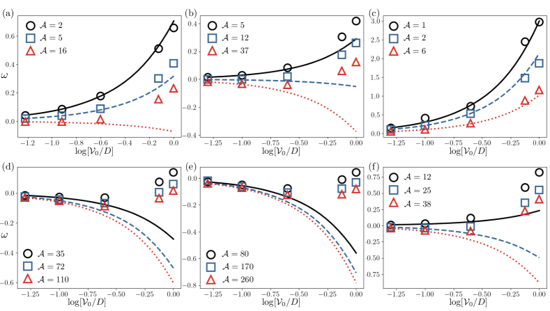
Figure 6: Asymptotic behaviors of the wave speed $\omega$ vs. $\log(\mathcal{V}_{0}/D)$, where $\mathcal{V}_{0}/D\in[0.05,1.0]$. The markers represent simulations of the reduced 1D system (56) and (70), and the corresponding colored curves give the analytical value of $\omega^{(1)}$ computed from Eq. (112). We note the close agreement between Eq. (112) and the simulation results when $\mathcal{V}_{0}/D$ is small. When $\mathcal{A}$ is small, the agreement is reasonable even for large $\mathcal{V}_{0}/D$.

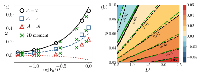
Figure 7: Simulations of the reduced 1D moment system (56) and (70) and the 2D moment equations (51)-(55) show quantitative agreement between the behavior of the two systems near the traveling wave solutions. (a) Comparison of the results of Fig. 6a with the 2D moment equations, denoted with green crosses. (b) Comparison of the contour plot Fig. 4c (main paper) with simulations of the 2D moment equations, denoted with green dot-dash lines.

Appendix: Movies

• Movie 1: Relaxation of random initial data to equilibrium for sufficiently small active Ericksen number (here, $(\mbox{Er}_{a},\mathcal{A})=(-0.1,0.06)$).

• Movie 2: The first flowing arrested state for immotile particles, emerging beyond a critical active Ericksen number (or particle concentration); $(\mbox{Er}_{a},\mathcal{A})=(-8,5)$ (Fig. 1b in the main paper).

• Movie 3: A fully two-dimensional flowing arrested state, for immotile particles with $(\mbox{Er}_{a},\mathcal{A})=(-16,10)$ (Fig. 1c in the main paper).

• Movie 4: A higher wavenumber dynamics and arrested state for of immotile particles at larger active Ericksen number, $\mathcal{V}_{0}=0$, with $(\mbox{Er}_{a},\mathcal{A})=(-70,45)$ and $\mathcal{W}=20$.

• Movie 5: Traveling wave for motile particles ($\mathcal{V}_{0}=0.06$) with $(\mbox{Er}_{a},\mathcal{A})=(-3,2)$ (Fig. 2a in the main paper).

• Movie 6: A retrograde traveling concentration wave with motile particles ($\mathcal{V}_{0}=0.06$) at larger active Ericksen number, with $(\mbox{Er}_{a},\mathcal{A})=(-7,37)$ (Fig. 2b in the main paper).

• Movie 7: A traveling periodic ‘thrashing’ mode emerges at larger swimming speeds ($\mathcal{V}_{0}=1$), with $(\mbox{Er}_{a},\mathcal{A})=(-15,10)$.

These movies may be viewed at: https://people.math.wisc.edu/~spagnolie/publications.html