Faster WIND:
Accelerating Iterative Best-of-$N$ Distillation for LLM Alignment

Abstract

Recent advances in aligning large language models with human preferences have corroborated the growing importance of best-of-$N$ distillation (BOND). However, the iterative BOND algorithm is prohibitively expensive in practice due to the sample and computation inefficiency. This paper addresses the problem by revealing a unified game-theoretic connection between iterative BOND and self-play alignment, which unifies seemingly disparate algorithmic paradigms. Based on the connection, we establish a novel framework, WIN rate Dominance (WIND), with a series of efficient algorithms for regularized win rate dominance optimization that approximates iterative BOND in the parameter space. We provides provable sample efficiency guarantee for one of the WIND variant with the square loss objective. The experimental results confirm that our algorithm not only accelerates the computation, but also achieves superior sample efficiency compared to existing methods.

Keywords: Reinforcement learning from human feedback (RLHF), preference optimization, matrix game, sample efficiency

1 Introduction

Fine-tuning large language models (LLMs) to align with human preferences has become a critical challenge in artificial intelligence to ensure the safety of their deployment. Reinforcement Learning from Human Feedback (RLHF) has emerged as a dominant approach, significantly improving LLM performance as demonstrated by InstructGPT (Ouyang et al., 2022) and subsequent works. RLHF combines reward modeling to quantify human preferences and RL fine-tuning to adjust the LLM’s output distribution, enhancing desired responses while suppressing unfavorable ones. While RLHF has shown promising results, it comes with significant extra post-training cost, and the aligned LLM may exhibit performance degeneration due to the alignment tax (Askell et al., 2021; OpenAI, 2023).

Alternatively, best-of-$N$ (BoN) sampling has emerged as a simple and surprisingly effective technique to obtain high-quality outputs from an LLM (Stiennon et al., 2020). In BoN sampling, multiple samples are drawn from an LLM, ranked according to a specific attribute, and the best one is selected. This simple approach can improve model outputs without the need for extensive fine-tuning, offering a potentially more efficient path to alignment. Building upon the success of BoN sampling, a few works explore the iterative variants of this approach (Dong et al., 2023; Sessa et al., 2024). Iterative BoN applies the sampling and selection process repeatedly, potentially leading to even better alignments with human preferences.

However, BoN incurs significant computational overhead due to making $n$ inference calls to generate one output, especially when $n$ is high. To mitigate the high inference cost of (iterative) BoN, Sessa et al. (2024) proposed a distillation algorithm, best-of-$N$ distillation (BOND), to train a new model emulating the output of iterative BoN. However, this approach also has a high training cost, due to the need of collecting multiple samples in each round of distillation, leading to a major bottleneck for wider adoption.

Given the growing importance and significance of the iterative BoN approach, it raises new questions about its theoretical properties, practical implementation, and relationship to established methods like RLHF. In this paper, we delve into the theoretical foundations and practical applications of iterative BoN sampling for LLM alignment. We address the following question:

What are the limiting points of iterative BoN, and can we design faster algorithms to find them?

1.1 Contributions

We provide comprehensive answers to these questions through the following key contributions:

• We introduce a general algorithmic framework for iterative BoN distillation, possibly with a slow moving anchor, and uncover its limiting point corresponds to the Nash equilibrium of a (regularized) two-player min-max game optimizing the logarithm of the expected win rate. This offers a fresh game-theoretic interpretation that is unavailable before.

• We show that the WIN rate Dominance (WIND) policy, which has a higher chance of winning against any other policy, solves the minmax game of win rate introduced in RLHF (Swamy et al., 2024; Munos et al., 2023), and approximates the iterative BoN’s limiting point.

• We propose a novel algorithm framework, WIND, to find the win rate dominance policy with flexible loss configurations, and demonstrate it exhibits improved sample and computation efficiency, compared to prior work while maintaining provable convergence guarantees.

• We conduct extensive experiments to evaluate the performance of WIND, demonstrating competitive or better performance against state-of-the-art alignment methods such as J-BOND across various benchmarks, highlighting its efficiency especially in the sampling process and training cost.

1.2 Related work

RLHF and LLM alignment.

Reinforcement Learning from human feedback (RLHF) is a effective approach to train AI models to produce outputs that aligns to human value and preference (Christiano et al., 2017; Stiennon et al., 2020; Nakano et al., 2021). Recently, RLHF has become the most effective approach to align language models (Ouyang et al., 2022; Bai et al., 2022). The famous InstructGPT (Ouyang et al., 2022) approach eventually led to the groundbreaking ChatGPT and GPT-4 (OpenAI, 2023). A variety of RLHF methods have been proposed, including the direct preference optimization (Rafailov et al., 2024) and many other variants (Zhao et al., 2023; Yuan et al., 2023b; Azar et al., 2024; Meng et al., 2024; Xu et al., 2024; Ethayarajh et al., 2024; Tang et al., 2024), to name a few, which directly learns from the preference data without RL finetuning. Furthermore, value-incentive preference optimization (Cen et al., 2024) has been proposed to implements the provably optimistic principle and pessimistic principle for exploration-exploitation tradeoff in a practical way.

RLHF via self-play.

One line of RLHF methods investigate self-play optimization for unregularized and regularized two-player win rate games, respectively (Swamy et al., 2024; Munos et al., 2023). Wu et al. (2024b) introduced a scalable self-play algorithm for win rate games, enabling efficient fine-tuning of LLMs, see also Rosset et al. (2024); Zhang et al. (2024) among others.

Best-of-$N$ and BOND.

BoN has empirically shown impressive reward-KL trade-off (Nakano et al., 2021; Gao et al., 2023), which has been theoretically investigated by Gui et al. (2024) from the win rate maximization perspective. Beirami et al. (2024) analyzed the KL divergence between the BoN policy and the base policy, and Yang et al. (2024a) studied the asymptotic properties of the BoN policy. The recent work Gui et al. (2024) also proposed a method to use both best-of-$N$ and worst-of-$N$ to train language models. Sessa et al. (2024) introduced BOND and J-BOND to train language models to learn BoN policies. Amini et al. (2024) proposed vBoN which is equivalent to BOND. However, there is no existing work for characterizing the properties of iterative BoN yet.

Notation.

We let $[n]$ denote the index set $\{1,\dots,n\}$. Let $I_{n}$ denote the $n\times n$ identity matrix, and inner product in Euclidean space $\mathbb{R}^{n}$ by $\langle\cdot,\cdot\rangle$. We let $\mathrm{supp}(\rho)$ denote the support set of the distribution $\rho$, and $\mathrm{relint}({\mathcal{C}})$ represents the relative interior of set ${\mathcal{C}}$. We defer all the proofs to the appendix.

2 Preliminaries

2.1 RLHF: reward versus win rate

We consider the language model $\pi_{\theta}(\cdot)$ as a policy, where $\theta\in\Theta$ denotes its parameters, and $\Theta$ the compact parameter space. Given a prompt $x\in\mathcal{X}$, the policy generates an answer $y\in\mathcal{Y}$ according to the conditional distribution $\pi_{\theta}(\cdot|x)$. For notation simplicity, we drop the subscript $\theta$ when it is clear from the context. We let $\Delta_{\mathcal{Y}}$ denote the simplex over $\mathcal{Y}$. We let $\Delta_{\mathcal{Y}}^{\mathcal{X}}$ denote the space of policies as follows:

$$\Delta_{\mathcal{Y}}^{\mathcal{X}}\coloneqq\big{\{}\pi=[\pi(\cdot|x)]_{x\in\mathcal{X}}\mid\pi(\cdot|x)\in\Delta_{\mathcal{Y}},\forall x\in{\mathcal{X}}\big{\}}.$$

In practice, RLHF optimize the policy model against the reward model while staying close to a reference model $\pi_{\textnormal{ref}}$. There are two metrics being considered: reward and win rate.

Reward maximization.

Suppose there is a reward model $r(x,y):\mathcal{X}\times\mathcal{Y}\mapsto\mathbb{R}$, which produce a scalar reward given a prompt $x$ and a response $y$. RLHF aims to maximize the KL-regularized value function, given a reference model $\pi_{\textnormal{ref}}$:

$$V_{\text{rm}}(\pi)=\underset{x\sim\rho,y\sim\pi(\cdot|x)}{\mathbb{E}}[r(x,y)]-\beta D_{\textnormal{KL}}\left(\pi\|\pi_{\textnormal{ref}}\right),$$ (1)

where

$$D_{\textnormal{KL}}\left(\pi_{1}\|\pi_{2}\right)=\mathbb{E}_{x\sim\rho}\left[\textnormal{KL}\left(\pi_{1}(\cdot|x)\|\pi_{2}(\cdot|x)\right)\right]$$

is the KL divergence between policies $\pi_{1}$ and $\pi_{2}$, with $\rho$ being the distribution of prompts. Here, $\beta\geq 0$ is a hyperparameter that balances the reward and the KL divergence. Without loss of generality, we assume $\mathrm{supp}(\rho)$ is ${\mathcal{X}}$ throughout the paper.

Win rate maximization.

Another scheme of RLHF aims to maximize the KL-regularized win rate against the reference model (Gui et al., 2024). Given a reward model $r$, a preference model $P_{x}:{\mathcal{Y}}\times{\mathcal{Y}}\rightarrow\{0,1/2,1\}$ can be defined as:

$$P_{x}(y,y^{\prime})\coloneqq\begin{cases}1,\,\,\text{ if $r(x,y)>r(x,y^{\prime})$,}\\ 1/2,\,\,\text{ if $r(x,y)=r(x,y^{\prime})$,}\\ 0,\,\,\text{ if $r(x,y)<r(x,y^{\prime})$.}\end{cases}$$ (2)

Given a policy pair $\pi,\pi^{\prime}$, the win rate of $\pi$ over $\pi^{\prime}$ is thus (Swamy et al., 2024)

$$P(\pi\succ\pi^{\prime}) \coloneqq\underset{x\sim\rho,y\sim\pi(\cdot|x),\atop y^{\prime}\sim\pi^{\prime}(\cdot|x)}{{\mathbb{E}}}P_{x}(y,y^{\prime})$$

$$=\mathbb{E}_{x\sim\rho}\pi^{\top}(\cdot|x)P_{x}(\cdot,\cdot)\pi^{\prime}(\cdot|x).$$ (3)

The KL-regularized win rate maximization objective is defined as (Gui et al., 2024):

$$V_{\text{wr}}(\pi)\coloneqq P(\pi\succ\pi_{\textnormal{ref}})-\beta D_{\textnormal{KL}}\left(\pi\|\pi_{\textnormal{ref}}\right).$$ (4)

The win rate maximization is more aligned with evaluation metric adopted in common benchmarks, and further, can be carried out without explicit reward models as long as the preference model $P_{x}$ is well-defined.

2.2 Best-of-$N$ distillation

Best-of-$N$ (BoN) is a simple yet strong baseline in RLHF. Given a reward model $r$ and a prompt $x$, BoN samples $n$ i.i.d. responses $y_{1},y_{2},...,y_{n}$ from the policy $\pi(\cdot|x)$ and select the response

$$y=\arg\max_{y\in y_{1},y_{2},...,y_{n}}r(x,y),\quad y_{1},\dots,y_{n}\sim\pi(\cdot|x)$$

with the highest reward. We call $\pi^{(n)}$ the BoN policy which selects the sample with the highest reward given $n$ samples i.i.d. drawn from $\pi$. Gui et al. (2024) shows that for any fixed small $\beta>0$, $\pi_{\textnormal{ref}}^{(n)}$ (approximately) maximizes $V_{\text{wr}}(\cdot)$ for properly chosen $n$. While BoN is widely used in practice (Beirami et al., 2024; Gao et al., 2023; Wang et al., 2024), yet can be quite expensive in terms of the inference cost for drawing $n$ samples. Hence, BoN distillation (BOND) (Sessa et al., 2024) is developed to approximate the BoN policy $\pi^{(n)}$ through fine-tuning from some reference policy $\pi_{\textnormal{ref}}(\cdot|x)$, which can be updated iteratively via an exponential moving average (Sessa et al., 2024).

3 A Unified Game-Theoretic View

In this section, we present a game-theoretic understanding of iterative BoN, which allows us to connect it to existing game-theoretic RLHF approaches under a win rate maximization framework.

3.1 Iterative BoN as game solving

Iterative BoN.

Due to the success of BoN sampling, its iterative version has also been studied (Dong et al., 2023; Sessa et al., 2024), where BoN is performed iteratively by using a moving anchor as the reference policy. To understand its property in generality, we introduce the iterative BoN method in Algorithm 1 that encapsulates iterative BoN methods with or without moving reference model, which we call the mixing and no-mixing case.

Algorithm 1 Iterative BoN

1:  Input: reference policy $\pi_{\textnormal{ref}}$, iterate number $T$, Best-of-$N$ parameter $n$, boolean value Mixing.

2:  Optional: mixing rates $\alpha_{1}>0,\alpha_{2}\geq 0$ such that $\alpha_{1}+\alpha_{2}\leq 1$.

3:  Initialization: $\pi_{0}\leftarrow\pi_{\textnormal{ref}}$.

4:  for $t=0,1,\cdots,T-1$ do

5:     $\pi_{t}^{(n)}\leftarrow\textrm{Best-of-$N$}(\pi_{t},n)$.

6:     if Mixing then

7:        $\pi_{t+1}\propto(\pi_{t}^{(n)})^{\alpha_{1}}\pi_{t}^{\alpha_{2}}\pi_{\textnormal{ref}}^{1-\alpha_{1}-\alpha_{2}}$;

8:     else if not Mixing then

9:        $\pi_{t+1}\leftarrow\pi_{t}^{(n)}$.

10:     end if

11:  end for

12:  Return $\pi_{T}$.

Algorithm 1 demonstrates these two cases. In the mixing case, we obtain new policies by mixing the BoN policy $\pi_{t}^{(n)}$, $\pi_{t}$ and $\pi_{\textnormal{ref}}$ at each iteration with mixing rates $\alpha_{1},\alpha_{2}$. In the no-mixing case, the algorithm simply returns the BoN policy $\pi_{t}^{(n)}$ as $\pi_{t+1}$ for the next iteration. We will provide some theoretical guarantees for both cases, using the following game-theoretic framework.

Game-theoretic perspective.

We show that iterative BoN is implicitly solving the following game. Define a preference matrix $\overline{P}_{x}$ at $x\in{\mathcal{X}}$ of size $|{\mathcal{Y}}|\times|{\mathcal{Y}}|$ by

$$\overline{P}_{x}(y,y^{\prime})\coloneqq\begin{cases}1,\,\,\text{ if $r(x,y)\geq r(x,y^{\prime})$,}\\ 0,\,\,\text{ if $r(x,y)<r(x,y^{\prime})$.}\end{cases}$$ (5)

Define further $f_{\beta}:\Delta_{\mathcal{X}}^{\mathcal{Y}}\times\Delta_{\mathcal{X}}^{\mathcal{Y}}\rightarrow\mathbb{R}$ as

$$f_{\beta}(\pi,\pi^{\prime}) \coloneqq\underset{x\sim\rho,\atop y\in\pi(\cdot|x)}{\mathbb{E}}\big{[}\log\underset{y^{\prime}\in\pi^{\prime}(\cdot|x)}{\mathbb{E}}\overline{P}_{x}(y\succeq y^{\prime})\big{]}-\beta D_{\textnormal{KL}}\left(\pi\|\pi_{\textnormal{ref}}\right).$$ (6)

We introduce the following symmetric two-player log-win-rate game:

$$\begin{cases}\pi_{1}=\arg\max_{\pi}f_{\beta}(\pi,\pi_{2}),&\\ \pi_{2}=\arg\max_{\pi}f_{\beta}(\pi,\pi_{1}).&\end{cases}$$ (7)

Let $\overline{\pi}^{\star}_{\beta}$ be a Nash equilibrium of the log-win-rate game (7), which satisfies the fixed-point characterization:

$$\overline{\pi}^{\star}_{\beta} \in\arg\max_{\pi}\underset{x\sim\rho,\atop y\in\pi(\cdot|x)}{\mathbb{E}}\big{[}\log\underset{y^{\prime}\in\overline{\pi}^{\star}_{\beta}(\cdot|x)}{\mathbb{E}}\overline{P}_{x}(y\succeq y^{\prime})\big{]}-\beta D_{\textnormal{KL}}\left(\pi\|\pi_{\textnormal{ref}}\right).$$ (8)

Now we present our Theorem 1, which guarantees the convergence to solutions for the above game under Algorithm 1.

Theorem 1 (Iterative BoN solves game (7)).

Let $\pi_{\textnormal{ref}}\in\text{relint}\left(\Delta_{\mathcal{Y}}^{\mathcal{X}}\right)$ and $n\geq 2$ in Algorithm 1. Then $\pi_{\infty}\coloneqq\lim_{T\rightarrow\infty}\pi_{T}$ exists, and $(\pi_{\infty},\pi_{\infty})$ is a Nash equilibrium of the log-win-rate game (7) when:

1. (no-mixing) $\alpha_{1}=1,\alpha_{2}=0$ for $\beta=0$;

2. (mixing) $\alpha_{1}=\frac{\eta}{(1+\beta\eta)(n-1)}$, $\alpha_{2}=\frac{n-1-\eta}{(1+\beta\eta)(n-1)}$ for any $\beta,\eta>0$.

In the no-mixing case, we can show that $\pi_{T}$ obtained by Algorithm 1 converges to the equilibrium of the unregularized log-win-rate game. In the mixing case, we show that with proper choice of mixing rates, Algorithm 1 solves the regularized log-win-rate game. To the best of our knowledge, this is the first game-theoretic understanding of iterative BoN using a general preference model.

3.2 Self-play and win rate dominance

The $\log$-win-rate game (7) is a non-zero-sum game that may be challenging to optimize: the function $f_{\beta}$ is not convex-concave, the Nash equilibria may not be unique, and the $\log$ term introduces nonlinearity, which induces difficulty in estimation. Therefore, we seek a good alternative to the $\log$-win-rate game that maintains its core properties while being more amenable to optimization.

Specifically, we now consider the following alternative two-player win-rate game:

$$\max_{\pi}\min_{\pi^{\prime}}P(\pi\succ\pi^{\prime}) -\beta D_{\textnormal{KL}}\left(\pi\|\pi_{\textnormal{ref}}\right)+\beta D_{\textnormal{KL}}\left(\pi^{\prime}\|\pi_{\textnormal{ref}}\right),$$ (9)

which eliminates the nonlinearity in reward, and has been recently studied by Swamy et al. (2024); Wu et al. (2024b) for $\beta=0$ and Munos et al. (2023) for $\beta>0$.

The following proposition guarantees the game (9) is well-defined and is equivalent to the following fixed point problem:

$$\begin{split}\pi^{\star}_{\beta}&\in\arg\max_{\pi}P(\pi\succ\pi^{\star}_{\beta})-\beta D_{\textnormal{KL}}\left(\pi\|\pi_{\textnormal{ref}}\right)\\ &=\underset{x\sim\rho,y\sim\pi(\cdot|x),\atop y^{\prime}\sim\pi^{\star}_{\beta}(\cdot|x)}{{\mathbb{E}}}\left[P_{x}(y,y^{\prime})-\beta\log\frac{\pi(y|x)}{\pi_{\textnormal{ref}}(y|x)}\right].\end{split}$$ (10)

Proposition 1 (existence of $\pi^{\star}_{\beta}$).

$\pi^{\star}_{\beta}$ exists and $(\pi^{\star}_{\beta},\pi^{\star}_{\beta})$ is the Nash equilibrium of the minmax game (9). Moreover, when $\beta>0$, $(\pi^{\star}_{\beta},\pi^{\star}_{\beta})$ is the unique Nash equilibrium.

Win rate dominance.

The fixed-point equation (10) identifies a policy with a higher winning probability against any other policy. For $\beta=0$, $\pi^{\star}_{0}$ satisfies $P(\pi\succ\pi^{\star}_{0})\leq 1/2$ for any $\pi$, ensuring it outperforms other policies. When $\beta>0$, the KL divergence term encourages $\pi^{\star}_{\beta}$ to remain close to $\pi_{\textnormal{ref}}$ while maintaining a high win rate. We term (10) the Win rate Dominance (WIND) optimization problem.

3.3 Connecting iterative BoN with WIND

Due to the monotonicity of $\log(\cdot)$, it is natural to believe the win rate game and the log-win-rate game beneath iterative BoN are connected. We establish the novel relationship rigorously, which allows a unifying game-theoretic view for many existing algorithms. We define a constant $c_{\beta}\in(0,+\infty]$ related to $\pi_{\textnormal{ref}}$:

$$c_{\beta}\coloneqq\min_{x\in{\mathcal{X}},\atop y\in{\mathcal{Y}}\backslash{\mathcal{Y}}^{\star}(x)}\left\{\frac{\sum_{y^{\star}\in{\mathcal{Y}}^{\star}(x)}\pi_{\textnormal{ref}}(y^{\star}|x)}{4\max\left\{\log\frac{\pi_{\textnormal{ref}}(y|x)}{\underset{y^{\star}\in{\mathcal{Y}}^{\star}(x)}{\max}\pi_{\textnormal{ref}}(y^{\star}|x)},0\right\}}\right\},$$ (11)

where ${\mathcal{Y}}^{\star}(x)\coloneqq\operatorname*{arg\,max}_{y\in{\mathcal{Y}}}r(x,y)$ is the set of optimal responses for each $x\in{\mathcal{X}}$. We now demonstrate the relationship between the equilibria set of the log-win-rate game $\overline{\pi}^{\star}_{\beta}$ and the win-rate game $\pi^{\star}_{\beta}$.

Theorem 2 (relationship between two games (informal)).

Let $\pi_{\textnormal{ref}}\in\text{relint}\left(\Delta_{\mathcal{Y}}^{\mathcal{X}}\right)$ and $n\geq 2$ in Algorithm 1. Then

• When $\beta=0$, $\overline{\pi}^{\star}_{\beta}$ is also a solution to (10);

• When $\beta\in(0,c_{\beta})$ where $c_{\beta}$ is defined in (11), for all $x\in{\mathcal{X}}$, $\overline{\pi}^{\star}_{\beta}$ satisfies

  $$\left\|\overline{\pi}^{\star}_{\beta,x}-\pi^{\star}_{\beta,x}\right\|_{1}\leq 4(|{\mathcal{Y}}|-|{\mathcal{Y}}^{\star}(x)|)\exp\Big{(}\frac{-\sum_{y^{\star}\in{\mathcal{Y}}^{\star}(x)}\pi_{\textnormal{ref}}(y^{\star}|x)}{4\beta}\Big{)}\rightarrow 0\text{ as }\beta\rightarrow 0.$$ (12)

Theorem 2 shows when $\beta=0$, both games have the solution $\overline{\pi}^{\star}_{0}$. For small positive $\beta$, the $\ell_{1}$ distance between the solutions of the two games is bounded by a term that decreases exponentially with $1/\beta$. We verify Theorem 2 empirically on contextual bandits in Section 5.1.

This result provides theoretical justification for using iterative BoN as an approximation to WIND, especially when $\beta$ is small. More importantly, it paves a way for efficient algorithm to WIND, bypassing the $\log$ operator in the win-rate game.

4 Faster WIND

Based on the understanding of the connection between $\log$-win-rate game and win-rate game, in this section, we propose a new sample-efficient algorithm for finding the WIND solution in (9), which includes two ingredients: (i) identifying a memory-efficient, exact policy optimization algorithm with linear last-iterate convergence (Sokota et al., 2023), and (ii) developing a series of sample-efficient algorithms with flexible loss functions and finite-time convergence guarantee. With slight abuse of terminology, we shall refer to our algorithmic framework WIND.

4.1 Exact policy optimization with last-iterate linear convergence

Recognizing that (9) is an KL-regularized matrix game, there are many existing algorithms that can be applied to find $\pi^{\star}_{\beta}$. Nonetheless, it is desirable to achieve fast last-iterate convergence with a small memory footprint. This is especially important in LLM optimization, for the memory efficiency. For example, extragradient algorithms (e.g., Korpelevich (1976); Popov (1980); Cen et al. (2021))—although fast-convergent—are expected to be expensive in terms of memory usage due to the need of storing an additional extrapolation point (i.e., the LLM) in each iteration.

It turns out that the magnetic mirror descent algorithm in Sokota et al. (2023), which is proposed to solve an equivalent variational inequality formulation to (9), meets our consideration. We present a tailored version of this algorithm in Algorithm 2, and state its linear last-iterate convergence in Theorem 3.

Algorithm 2 WIND (exact gradient, adapted from Sokota et al. (2023) tailored for our setting)

1:  Input: reference policy $\pi_{\textnormal{ref}}$, initial policy $\pi^{(0)}$, regularization coefficient $\beta>0$, learning rate $\eta>0$.

2:  for $t=0,1,\cdots$ do

3:     Update $\pi(\cdot|x)$ for all $x\in{\mathcal{X}}$:

$$\pi^{(t+1)}(y|x)\propto(\pi^{(t)}(y|x))^{\frac{1}{1+\beta\eta}}(\pi_{\textnormal{ref}}(y|x))^{\frac{\beta\eta}{1+\beta\eta}}\exp\left(\frac{\eta}{1+\beta\eta}\mathbb{E}_{y^{\prime}\sim\pi^{(t)}(\cdot|x)}P_{x}(y,y^{\prime})\right)$$ (13)

4:  end for

Theorem 3 (Linear last-iterate convergence of Algorithm 2, Sokota et al. (2023)).

Assume $\beta>0$ and $\pi^{(0)},\pi_{\textnormal{ref}}\in\text{relint}(\Delta^{\mathcal{X}}_{\mathcal{Y}})$.When the learning rate $\eta\in(0,\beta]$, $\pi^{(t)}$ in Algorithm 2 satisfies:

$$D_{\mathrm{KL}}\big{(}\pi^{\star}_{\beta}||{\pi^{(t)}}\big{)}\leq\bigg{(}\frac{1}{1+\eta\beta}\bigg{)}^{t}D_{\textnormal{KL}}\left(\pi^{\star}_{\beta}\|\pi^{(0)}\right).$$ (14)

Remark 1.

We note that when $\beta=0$, the update rule (13) recovers (Swamy et al., 2024, Algorithm 1). When $\beta>0$, the update rule in (13) is different from that of Munos et al. (2023), which is

$$\pi^{(t+1)}(y|x) \propto\widetilde{\pi}^{(t)}(y|x)\cdot\exp\left(\eta{\mathbb{E}}_{y^{\prime}\sim\widetilde{\pi}^{(t)}(\cdot|x)}P_{x}(y,y^{\prime})\right),$$

where $\widetilde{\pi}^{(t)}$ is a mixed policy defined as

$$\widetilde{\pi}^{(t)}(y|x)\propto\big{(}\pi^{(t)}(y|x)\big{)}^{1-\eta\beta}\left(\pi_{\textnormal{ref}}(y|x)\right)^{\eta\beta}.$$

As such, it requires extra memory to store $\widetilde{\pi}^{(t)}$. Moreover, Munos et al. (2023) shows a slower rate of ${\mathcal{O}}(1/T)$, whereas Algorithm 2 admits linear convergence.

4.2 Sample-efficient algorithm

We now derive practical sample-efficient methods for approximating the exact update (13) of WIND in the parameter space $\Theta$ of the policy $\pi_{\theta}$, $\theta\in\Theta$. For exposition, we use $\phi_{\theta}$ to denote the logits before softmax, i.e.,

$$\pi_{\theta}=\mathsf{softmax}\circ\phi_{\theta},$$

where $\mathsf{softmax}(x)_{i}\coloneqq e^{x_{i}}/\sum_{j}e^{x_{j}}$ is the softmax function.

We consider the existence of reward model approximation error, i.e., we may use an inaccurate judger $\widehat{P}_{x}$, which is an approximation of $P_{x}$. For example, instead of training a reward model, we could use an LLM $\widehat{P}$ as a judger to directly judge if response $y$ is better than $y^{\prime}$ or not given a prompt $x$, and use $\widehat{P}_{x}$ as an approximation of $P_{x}$.

Algorithm derivation with the squared risk.

Let $\theta_{t},\theta_{\text{ref}}$ denote the parameters of $\pi^{(t)}$ and $\pi_{\textnormal{ref}}$ in Algorithm 2, respectively. We rewrite the update rule (13) as

$$\phi_{\theta_{t+1}}(y|x) =\frac{1}{1+\beta\eta}\phi_{\theta_{t}}(y|x)+\frac{\beta\eta}{1+\beta\eta}\phi_{\theta_{\textnormal{ref}}}(y|x)+\frac{\eta}{1+\beta\eta}\mathbb{E}_{y^{\prime}\sim\pi_{\theta_{t}}(\cdot|x)}P_{x}(y,y^{\prime})+Z_{t}(x)$$ (15)

for some function $Z_{t}:{\mathcal{X}}\rightarrow\mathbb{R}$. We define a proxy $\varphi_{t}:{\mathcal{X}}\times{\mathcal{Y}}\times{\mathcal{Y}}\rightarrow\mathbb{R}$ using the empirical win-rate as

$$\varphi_{t}(x,y,y^{\prime}) \coloneqq\frac{1}{1+\beta\eta}\phi_{\theta_{t}}(y|x)+\frac{\beta\eta}{1+\beta\eta}\phi_{\theta_{\textnormal{ref}}}(y|x)+\frac{\eta}{1+\beta\eta}\widehat{P}_{x}(y,y^{\prime})+Z_{t}(x),$$ (16)

Our observation is that the update (15) of $\phi_{\theta_{t}}(y|x)$ is approximating the conditional expectation of $\varphi_{t}$, which is

$$\psi_{t}(x,y)\coloneqq\mathbb{E}_{y^{\prime}\sim\pi_{\theta_{t}}(\cdot|x)}[\varphi_{t}(x,y,y^{\prime})|x,y],\,\,\forall(x,y).$$

Furthermore, this conditional expectation has the lowest risk, due to the following lemma:

Lemma 1 (Conditional mean minimizes the square loss).

For any two random variables $u,v$, we have

$$\mathbb{E}_{u,v}\left[(v-\mathbb{E}_{v}(v|u))^{2}\right]\leq\mathbb{E}_{u,v}\left[(v-g(u))^{2}\right]$$ (17)

for any function $g$. In particular, the equality holds if and only if $g(u)=\mathbb{E}_{v}(v|u)$ almost everywhere on the support of the distribution of $u$.

To invoke Lemma 1, we assume the LLM is expressive enough, such that $\psi_{t}$ can be represented by $\phi_{\theta}$:

Assumption 1 (expressive power).

For any $t\in{\mathbb{N}}$, there exists $\theta_{t+1}^{\star}\in\Theta$ such that

$$\forall(x,y)\in{\mathcal{X}}\times{\mathcal{Y}}:\quad\phi_{\theta_{t+1}^{\star}}(y|x)=\psi_{t}(x,y).$$ (18)

Note that $\mathrm{supp}(\rho)={\mathcal{X}}$, $\mathrm{supp}(\pi^{(t)}(\cdot|x))={\mathcal{Y}}$ for all $x\in{\mathcal{X}}$, $t\in{\mathbb{N}}$. Thus under Assumption 1, by Lemma 1 we know that for all $t$, $\theta_{t+1}^{\star}\in\Theta$ satisfies (18) if and only if

$$\theta_{t+1}^{\star}\in\operatorname*{arg\,min}_{\theta\in\Theta}R_{t}(\theta),$$ (19)

where we define the squared expected risk at the $t$-th iteration $R_{t}^{\textnormal{sq}}(\theta)$ as

$$R_{t}^{\textnormal{sq}}(\theta)\coloneqq\underset{x\sim\rho,\atop y,y^{\prime}\sim\pi_{\theta_{t}}(\cdot|x)}{\mathbb{E}}\left[\left(\varphi_{t}(x,y,y^{\prime})-\phi_{\theta}(y|x)\right)^{2}\right].$$

In implementation, at each iteration $t$, we shall approximate $\theta_{t+1}^{\star}$ by minimizing the empirical risk: we sample $x_{i}^{(t)}\sim\rho$, $y_{i}^{(t)},{y_{i}^{\prime}}^{(t)}\sim\pi_{\theta_{t}}(\cdot|x_{i}^{(t)})$, $i\in[M]$, and compute $\theta_{t+1}$ by minimizing the empirical risk $R^{\textnormal{sq}}_{t,M}(\theta)$ defined as

$$R_{t,M}^{\textnormal{sq}}(\theta) \coloneqq\frac{1}{M}\sum_{i=1}^{M}\big{(}\varphi_{t}(x_{i}^{(t)},y_{i}^{(t)},{y_{i}^{\prime}}^{(t)})-\phi_{\theta}(y_{i}^{(t)}|x_{i}^{(t)})\big{)}^{2}.$$ (SQ)

We summarize the update procedure in Algorithm 3.

Algorithm 3 WIND (sample-efficient version)

1:  Input: reference parameter $\theta_{\textnormal{ref}}$, initial parameter $\theta_{0}$, regularization coefficient $\beta>0$, learning rate $\eta>0$, training set ${\mathcal{D}}$, iteration number $T\in{\mathbb{N}}_{+}$, sampling number $M\in{\mathbb{N}}_{+}$.

2:  for $t=0,1,\cdots,T-1$ do

3:     Sample $x_{i}^{(t)}\sim\rho$, $y_{i}^{(t)},{y_{i}^{\prime}}^{(t)}\sim\pi_{\theta_{t}}(\cdot|x_{i}^{(t)})$, $i\in[M]$.

4:     $\theta_{t+1}\leftarrow\operatorname*{arg\,min}_{\theta\in\Theta}R_{t,M}(\theta).$ $\triangleright$ $R_{t,M}$ could be $R_{t,M}^{\textnormal{sq}}$, $R_{t,M}^{\textnormal{kl}}$, $R_{t,M}^{\textnormal{nce}}$, etc.

5:  end for

6:  Return $\theta_{T}$.

Alternative risk functions.

By utilizing different variational forms, we could derive objectives different from (SQ). For illustration, we provide two alternatives of $R^{\textnormal{sq}}_{t,M}(\theta)$ by using the KL divergence and NCE loss, respectively (see Appendix A for derivations):

$$R_{t,M}^{\textnormal{kl}}(\theta) \coloneqq-\frac{1}{M}\sum_{i=1}^{M}\big{[}\mathbbm{1}_{\{v_{i}=1\}}\log\zeta_{\theta}(x,y)+\mathbbm{1}_{\{v_{i}=0\}}\log(1-\zeta_{\theta}(x,y))\big{]},$$ (KL)

and

$$R_{t,M}^{\textnormal{nce}}(\theta)\coloneqq-\frac{1}{M}\sum_{i=1}^{M}\Big{[}\left(\mathbbm{1}_{\{v_{i}=1\}}+\mathbbm{1}_{\{v_{i}^{\prime}=0\}}\right)\log\frac{\zeta_{\theta}(x_{i},y_{i})}{\zeta_{\theta}(x_{i},y_{i})+p}+\left(\mathbbm{1}_{\{v_{i}=0\}}+\mathbbm{1}_{\{v_{i}^{\prime}=1\}}\right)\log\frac{p}{\zeta_{\theta}(x_{i},y_{i})+p}\Big{]},$$ (NCE)

where $v_{i}\sim\mathsf{Ber}(\widehat{P}_{x_{i}}(y_{i},y_{i}^{\prime}))$, $v_{i}^{\prime}\sim\mathsf{Ber}(p)$, $p\in(0,1)$ is a hyperparameter, $\zeta_{\theta}$ is defined as

$$\zeta_{\theta}(x,y) =\frac{1+\beta\eta}{\eta}\phi_{\theta}(y|x)-\frac{1}{\eta}\phi_{\theta_{t}}(y|x)-\beta\phi_{\theta_{\textnormal{ref}}}(y|x)-\frac{1+\beta\eta}{\eta}Z_{t}(x),$$

and $\mathbbm{1}_{\{A\}}$ is the indicator function that equals 1 if $A$ is true and 0 otherwise.

When we use the regression objective (SQ), our WIND algorithm shares a similar form to SPPO (Wu et al., 2024b). However, WIND differs from SPPO in the following aspects: (i) we solve the regularized game with the KL regularization term $\beta D_{\textnormal{KL}}\left(\pi^{\prime}\|\pi_{\textnormal{ref}}\right)$. This term is crucial in practice and is also considered in other iterative BOND methods (Dong et al., 2023; Sessa et al., 2024); (ii) our sampling scheme is more sample-efficient: in SPPO, for each $x_{i}$, they sample $K$ responses $\{y_{i,j}\}_{j\in[K]}$ to estimate $\mathbb{E}_{y^{\prime}\sim\pi_{\theta_{t}}(\cdot|x_{i})}[P_{x_{i}}(y_{i,j},y^{\prime})]$ by $\frac{1}{K}\sum_{k=1}^{K}P_{x_{i}}(y_{i,j},y_{i,k})$ for each $j\in[K]$. On the other hand, Lemma 1 implies estimating the conditional mean with multiple samples is unnecessary and for each $x_{i}$, sampling two responses $y_{i}$ and $y_{i}^{\prime}$ is enough; (iii) we allow different risk functions beyond the squared loss.

4.3 Convergence analysis

We provide a finite-sample complexity guarantee for Algorithm 3 when the risk $R_{t,M}=R_{t}^{\textnormal{sq}}$. Our results could be easily extended to other risks. Here we consider the existence of reward model approximation error, i.e., we may use an inaccurate judger $\widehat{P}_{x}$ as an approximation of $P_{x}$. For example, instead of training a reward model, we could use an LLM $\widehat{P}$ as a judger to directly judge if response $y$ is better than $y^{\prime}$ or not given a prompt $x$, and use $\widehat{P}_{x}$ as an approximation of $P_{x}$.

We define the model approximation error $\delta_{P}$ as

$$\delta_{P}\coloneqq\max_{x\in{\mathcal{X}},y,y^{\prime}\in{\mathcal{Y}}}\left|P_{x}(y,y^{\prime})-\widehat{P}_{x}(y,y^{\prime})\right|.$$ (20)

We require the following assumptions to prove the convergence of Algorithm 3. The first assumes $\phi_{\theta}$ is differentiable and $\Theta$, $Z_{t}$ is bounded.

Assumption 2 (differentiability and boundedness).

The parameter space $\Theta$ is compact, $\phi_{\theta}(y|x)$ is differentiable w.r.t. $\theta$ for any $(x,y)\in{\mathcal{X}}\times{\mathcal{Y}}$, and $Z_{t}$ in (15) is uniformly bounded, i.e., $\exists Z\geq 0$ such that $|Z_{t}(x)|\leq Z$ for all $x\in{\mathcal{X}}$ and $t\in{\mathbb{N}}$.

Assumption 2 guarantees the (uniform) boundedness of $\phi_{\theta}$. Especially, there exists $L_{0}>0$ such that for any $\theta,\theta^{\prime}\in\Theta$ and $(x,y)\in{\mathcal{X}}\times{\mathcal{Y}}$, we have

$$|\phi_{\theta}(y|x)-\phi_{\theta^{\prime}}(y|x)|\leq L_{0}.$$ (21)

Assumption 2 also guarantees there exist $L,C>0$ such that for all $x\in{\mathcal{X}},y,y^{\prime}\in{\mathcal{Y}},\theta\in\Theta$ and $t$, we have

$$\left\|\nabla_{\theta}\left[\left(\varphi_{t}(x,y,y^{\prime})-\phi_{\theta}(y|x)\right)^{2}\right]\right\|_{2}\leq L.$$ (22)

and

$$\left(\varphi_{t}(x,y,y^{\prime})-\phi_{\theta}(y|x)\right)^{2}\leq C.$$ (23)

The next assumption controls the concentrability coefficient, which is commonly used in the RL literature, see Yuan et al. (2023a); Munos (2003, 2005); Munos and Szepesvári (2008); Yang et al. (2023) for example.

Assumption 3 (concentrability coefficient).

For Algorithm 3, there exists finite $C_{\pi}>0$ such that for all $t\in{\mathbb{N}}$ and $x\in{\mathcal{X}}$, we have

$$\mathbb{E}_{y\sim\pi_{\textnormal{ref}}(\cdot|x)}\left[\left(\frac{\pi^{\star}_{\beta}(y|x)}{\pi_{\textnormal{ref}}(y|x)}\right)^{2}\right]\leq C_{\pi}\qquad\mbox{and}\qquad\mathbb{E}_{y\sim\pi_{\textnormal{ref}}(\cdot|x)}\left[\left(\frac{\pi_{\theta_{t+1}}(y|x)}{\pi_{\textnormal{ref}}(y|x)}\right)^{2}\right]\leq C_{\pi}.$$

We define

$$C_{1}\coloneqq\exp\left(\frac{2}{\beta}\left(\delta_{P}+\frac{1+\beta\eta}{\eta}L_{0}+1\right)\right)C_{\pi}.$$ (24)

We also assume for every $t$, the expected risk $R_{t}$ and empirical risk $R_{t,N}$ both satisfy Polyak-Łojasiewicz (PL) condition, which has been proven to hold for over-parameterized neural networks including transformers (Liu et al., 2022; Wu et al., 2024a; Yang et al., 2024b).

Assumption 4 (Polyak-Łojasiewicz condition).

For all $t\in{\mathbb{N}}$, risk $R_{t}$ and empirical risk $R_{t,M}$ both satisfy Polyak-Łojasiewicz condition with parameter $\mu>0$, i.e., for all $t\in{\mathbb{N}}$ and $\theta\in\Theta$, we have

$$\frac{1}{2}\left\|\nabla_{\theta}R_{t}(\theta)\right\|_{2}^{2}\geq\mu\left(R_{t}(\theta)-R_{t}(\theta_{t+1}^{\star})\right)$$

and

$$\frac{1}{2}\left\|\nabla_{\theta}R_{t,N}(\theta)\right\|_{2}^{2}\geq\mu\left(R_{t,M}(\theta)-R_{t,M}(\theta_{t+1})\right).$$

Remark 2 (Assumption 4 is satisfied with linear function approximation).

We consider a special case where $\phi_{\theta}(y|x)=\phi(x,y)^{\top}\theta$ for all $(x,y)\in{\mathcal{X}}\times{\mathcal{Y}}$, where $\phi(x,y)$ are the feature maps. If for all $t\in{\mathbb{N}}$, we have

$$\mathbb{E}_{x\sim\rho,y\sim\pi_{\theta_{t}}(\cdot|x)}\big{[}\phi(x,y)\phi(x,y)^{\top}\big{]}\geq\frac{\mu}{2}$$

and

$$\frac{1}{M}\sum_{i=1}^{M}\phi(x_{i}^{(t)},y_{i}^{(t)})\phi(x_{i}^{(t)},y_{i}^{(t)})^{\top}\geq\frac{\mu}{2},$$

then it’s straightforward to verify that $R_{t}$ and $R_{t,M}$ are both $\mu$-strongly convex, which indicates Assumption 4 holds (Karimi et al., 2016).

The following theorem gives the convergence of Algorithm 3.

Theorem 4 (Convergence of Algorithm 3).

Let $\theta_{0}=\theta_{\textnormal{ref}}$ and $\eta\in(0,\beta]$ in Algorithm 3. Under Assumption 1,2,3,4, for any $T\in{\mathbb{N}}$ and $\delta\in(0,1)$, with probability at least $1-\delta$, Algorithm 3 satisfies:

$$D_{\textnormal{KL}}\left(\pi^{\star}_{\beta}\|\pi_{\theta_{T}}\right) \leq\left(\frac{1}{1+\beta\eta}\right)^{T}D_{\textnormal{KL}}\left(\pi^{\star}_{\beta}\|\pi_{\theta_{0}}\right)$$

$$\quad+\frac{2}{\beta}\delta_{P}+\frac{2(1+\beta\eta)}{\beta\eta}\sqrt{C_{1}C_{r}\log\left(\frac{T}{\delta}\right)}\sqrt{\frac{2L^{2}\log M}{\mu(M-1)}+\frac{C+2L^{2}/\mu}{M}},$$ (25)

where $C_{r}$ is an absolute constant, $C_{1}$, $L$, $\delta_{P}$, $C$, $\mu$ are defined in (24), (22), (20), (23), Assumption 4, respectively.

Theorem 4 indicates that, assuming no model approximation error, the total sample complexity for Algorithm 3 to reach $\varepsilon$-accuracy is

$$2MT=\widetilde{O}\left(\left(\frac{1+\beta\eta}{\beta\eta}\right)^{2}\left(\frac{L^{2}}{\mu}+C\right)C_{1}C_{r}\frac{1}{\varepsilon^{2}}\right).$$

In contrast with SPPO (Wu et al., 2024b), which only ensures average-iterate convergence without quantifying sample efficiency, our method has stronger theoretical guarantees, offering last-iterate convergence and explicit sample complexity bounds.

5 Experiments

We report our experiment results in this section.

5.1 Contextual bandits

In this section we conduct contextual bandit experiments to validate Theorem 2.

Experiments setup.

We set $|\mathcal{X}|=20,|\mathcal{Y}|=100$, and initialize $r(x_{i},y_{j})\overset{i.i.d}{\sim}{\mathcal{N}}(0,1)$, where $i\in[|\mathcal{X}|],j\in[|\mathcal{Y}|]$, and ${\mathcal{N}}(0,1)$ stands for the standard Gaussian distribution. We set $\pi_{\textnormal{ref}}$ and $\rho$ to be uniform distributions and randomly initialized $\pi^{(0)}$ in Algorithm 2 using the Dirichlet distribution with parameters all set to be 1. For the distance metric, we use the average $\ell_{1}$ distance $D_{\ell_{1}}:\Delta^{{\mathcal{X}}}_{{\mathcal{Y}}}\times\Delta_{{\mathcal{Y}}}^{{\mathcal{X}}}\rightarrow\mathbb{R}$ defined as

$$D_{\ell_{1}}(\pi,\pi^{\prime})\coloneqq\mathbb{E}_{x\sim\rho}\left\|\pi_{x}-\pi^{\prime}_{x}\right\|_{1}.$$ (26)

We conduct the following two experiments:

• For the no-mixing case where $\alpha_{1}=1,\alpha_{2}=0$, we show the convergence of both iterative BoN (c.f. Algorithm 1) and exact WIND (c.f. Algorithm 2) to $\overline{\pi}^{\star}_{0}$: we plot the average $\ell_{1}$ distance between $\overline{\pi}^{\star}_{0}$ and the iterates for both algorithms. In this experiments we set learning rate $\eta$ in Algorithm 2 to be 16.

• For the mixing case where $\alpha_{1}=\frac{\eta}{(1+\beta\eta)(n-1)}$ and $\alpha_{2}=\frac{n-1-\eta}{(1+\beta\eta)(n-1)}$, we verify that $\overline{\pi}^{\star}_{\beta}$ and $\pi^{\star}_{\beta}$ are very close to each other: we fix the iteration number $T=5000$ for both Algorithm 1 and 2, and increase $\beta$ from 0.01 to 0.1 to plot the change of average $\ell_{1}$ distance between the final outputs of the two algorithms $D_{\ell_{1}}(\pi_{T},\pi^{(T)})$ with respect to $\beta$. In this experiments we set $\eta=1$.

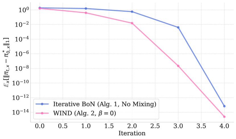
(a) no-mixing

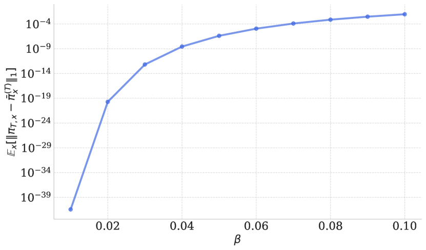
(b) mixing

Figure 1: Empirical validation of Theorem 2 on contextual bandit experiments. For (a) the no-mixing case, we show the convergence of both iterative BoN (c.f. Algorithm 1) and exact WIND (c.f. Algorithm 2) to $\overline{\pi}^{\star}_{0}$; for (b) the mixing case, we show $\overline{\pi}^{\star}_{\beta}$ and $\pi^{\star}_{\beta}$ are very close to each other.

Results.

Our results are presented in Figure 1. Figure 1(a) indicates that for the no-mixing case, both algorithms converge to $\overline{\pi}^{\star}_{0}$ with WIND slightly faster than iterative BoN. From Figure 1(b), we can see that $\overline{\pi}^{\star}_{\beta}$ and $\pi^{\star}_{\beta}$ are very close to each other when $\beta$ is small and their distance approaches 0 very quickly as $\beta\rightarrow 0$, which corroborates (12).

Model	GSM8k	HellaSwag	MMLU	MT-Bench
				1st Turn	2nd Turn	Avg
Llama-3-8B-SPPO Iter1	75.44	79.80	65.65	8.3813	7.6709	8.0283
Llama-3-8B-SPPO Iter2	75.13	80.39	65.67	8.3875	7.4875	7.9375
Llama-3-8B-SPPO Iter3	74.91	80.86	65.60	8.0500	7.7625	7.9063
Llama-3-8B-JBOND Iter1	76.12	77.70	65.73	8.2875	7.4281	7.8578
Llama-3-8B-JBOND Iter2	75.74	77.47	65.85	8.2563	7.4403	7.8495
Llama-3-8B-JBOND Iter3	76.12	77.36	65.83	8.2750	7.2767	7.7774
Llama-3-8B-WIND Iter1 (Ours)	75.82	78.73	65.77	8.2875	7.6875	7.9875
Llama-3-8B-WIND Iter2 (Ours)	76.19	79.05	65.77	8.3625	7.7500	8.0563
Llama-3-8B-WIND Iter3 (Ours)	77.18	79.31	65.87	8.5625	7.8354	8.2013

Table 1: Results on GSM8k, HellaSwag, MMLU and MT-Bench.

5.2 LLM alignment

We follow the experiment setup in Wu et al. (2024b) and Snorkel. We use Llama-3-8B-Instruct as the base pretrained model for baseline comparisons. For fair comparison, we chose the same prompt dataset UltraFeedback (Cui et al., 2023) and round splits, and the same Pair-RM framework (Jiang et al., 2023) for the preference model as in Wu et al. (2024b) and Snorkel. The learning rate is set to be $5\times 10^{-7}$. In each iteration, we generate answers from $20000$ prompts in the UltraFeedback dataset to train the model. The global training batch size is $64$ ($4$ per device $\times$ $16$ GPUs). Our experiments are run on $16$ A$100$ GPUs, where each has $40$ GB memory. We modify the per-device batch size and gradient accumulation steps in SPPO GitHub repository while keeping the actual training batch size, to avoid out-of-memory error.

Baselines and Benchmarks.

We consider two baselines: SPPO (Wu et al., 2024b) and a variant of J-BOND (Sessa et al., 2024). Here we follow the exact same setting in their repository of the SPPO paper to reproduce SPPO results, with the only change being that we use different computation devices.

We consider 4 major evaluation benchmarks: GSM8k, HellaSwag, MMLU and MT-Bench. They evaluated the following capability:

• GSM8k (Cobbe et al., 2021) evaluates the mathematical reasoning at a grade school level.

• HellaSwag (Zellers et al., 2019) measures the commonsense reasoning by letting language models select a choice to finish a half-complete sentence.

• MMLU (Hendrycks et al., 2020) is a large-scale benchmark that encompasses a variety of tasks to measure the language models’ knowledge.

• MT-Bench (Zheng et al., 2023) is also a LLM-as-a-judge benchmark that evaluates the LLM’s multi-round chat capability. The scores given by GPT-4 is reported.

Results.

For traditional benchmarks (GSM8k, HellaSwag and MMLU), which do not involve using LLMs as the judges, the results are shown in Table 1. The model Llama-3-8B-WIND of ours achieved optimal in the last iteration in GSM8k and MMLU, while performing better than the J-BOND variant and slightly worse than SPPO in HellaSwag. In fact, our method shows consistent improvement over iterations: for all three benchmarks, our method continues to improve with more iterations of training, while both SPPO and J-BOND variant show performance regressions with increasing number of iterations. For MT-Bench, Llama-3-8B-WIND achieves comparable results in comparison with SPPO, and outperforms J-BOND.

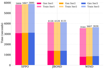
Figure 2: Run time (seconds) of different methods.

Runtime.

We also report the running time used by different methods in our setting. Since we base our implementation on the SPPO GitHub Repository, we only modify the objectives and the sampling process to reflect the difference between these algorithms. Figure 2 shows that our method achieves much better sample efficiency during data generation. In sum, the proposed WIND achieves superior performance with less computation cost, making iterative BOND practice applicable.

6 Conclusion

This work establishes a unified game-theoretic framework that connects iterative BoN with existing game-theoretic RLHF approaches. We present WIND, a sample-efficient efficient algorithm for win rate dominance optimization with finite-sample guarantees, which provides an accelerated alternative to iterative BOND. Empirical validation on multiple public benchmarks demonstrates the effectiveness and efficiency of our approach compared to several state-of-the-art methods.

Appendix A Other Objectives for Algorithm 3

In this section we give some possible alternative objectives for Algorithm 3 by utilizing different variational forms.

$f$-divergence objectives:

We could use $f$-divergence $D_{f}$ as the objective function. For a convex function $f$, $D_{f}$ is defined as

$$D_{f}(P||Q)\coloneqq\mathbb{E}_{Q}\left[f\left(\frac{P}{Q}\right)\right].$$ (27)

Let

$$U=(x,y)\quad\text{and}\quad V=\begin{cases}1,\text{ if $r(x,y)>r(x,y^{\prime})$,}\\ 0,\text{ if $r(x,y)<r(x,y^{\prime})$,}\\ z\sim Ber(1/2),\text{ if $r(x,y)=r(x,y^{\prime})$,}\end{cases}$$

Then $V|U$ is a function of $y^{\prime}$ and $P_{V|U}=Ber(\mathbb{E}_{y^{\prime}}P_{x}(y,y^{\prime}))$. Further define

$$\zeta_{\theta}(x,y)=\frac{1+\beta\eta}{\eta}\phi_{\theta}(y|x)-\frac{1}{\eta}\phi_{\theta_{t}}(y|x)-\beta\phi_{\theta_{\textnormal{ref}}}(y|x)-\frac{1+\beta\eta}{\eta}Z_{t}(x).$$ (28)

We let $Q_{V|U}=Ber(\zeta_{\theta}(y|x))$, then by solving

$$\theta_{t+1}=\arg\min_{\theta}\mathbb{E}_{U}D_{f}(P_{V|U}||Q_{V|U}),$$ (29)

we could approximate the update rule (15).

Especially, when $f(x)=x\log x$, we have $D_{f}=D_{\text{KL}}$, and (29) becomes

$$\theta_{t+1} =\arg\min_{\theta}\mathbb{E}_{x\sim\rho,y\sim\pi_{\theta_{t}}(\cdot|x)}\mathbb{E}_{v\sim P_{V|U}}\log\frac{P_{V|U}(v)}{Q_{V|U}(v)}$$

$$=\arg\min_{\theta}\mathbb{E}_{x\sim\rho,y\sim\pi_{\theta_{t}}(\cdot|x)}\mathbb{E}_{v\sim P_{V|U}}[-\log Q_{V|U}(v)].$$ (30)

We could approximate the above objective by sampling $x_{i}\sim\rho,y_{i},y_{i}^{\prime}\sim\pi_{\theta_{t}}(\cdot|x_{i})$ ($i\in[M]$) and minimizing the empirical risk:

$$\theta_{t+1}=\arg\min_{\theta}R_{t,M}^{\textnormal{kl}}(\theta)\coloneqq-\frac{1}{M}\sum_{i=1}^{M}\left[\mathbbm{1}_{\{v_{i}=1\}}\log\zeta_{\theta}(x,y)+\mathbbm{1}_{\{v_{i}=0\}}\log(1-\zeta_{\theta}(x,y))\right],$$ (31)

where

$$v_{i}=\begin{cases}1,\text{ if $r(x_{i},y_{i})>r(x_{i},y_{i}^{\prime})$,}\\ 0,\text{ if $r(x_{i},y_{i})<r(x_{i},y_{i}^{\prime})$,}\\ z\sim Ber(1/2),\text{ if $r(x_{i},y_{i})=r(x_{i},y_{i}^{\prime})$.}\end{cases}$$ (32)

For other $f$-divergence objectives, we may not be able to get rid of the unknown $P_{V|U}$ on the RHS of (29), but (29) could provide a gradient estimator for the objective that allows us to optimize $\theta$ by stochastic gradient descent.

Noise contrastive estimation (NCE) objectives.

We could use NCE (Gutmann and Hyvärinen, 2010) as objectives. NCE is a method to estimate the likelihood of a data point by contrasting it with noise samples. Let $D_{\theta}$ be the discriminator (parameterized by $\theta$) that distinguishes the true data from noise samples. The NCE objective is

$$\min_{\theta}\mathbb{E}_{z\sim P_{\textnormal{data}}}[-\log D_{\theta}(z)]+\mathbb{E}_{z\sim P_{\textnormal{noise}}}[-\log(1-D_{\theta}(z))],$$ (33)

Then the uptimal solution of (33) is

$$D_{\theta^{\star}}(z)=\frac{P_{\textnormal{data}}(z)}{P_{\textnormal{data}}(z)+P_{\textnormal{noise}}(z)}.$$

In our case, we let $P_{\textnormal{data}}=P_{V|U}$ and $P_{\textnormal{noise}}=Ber(p)$ where $p\in(0,1)$ is a hyperparameter. We also let

$$D_{\theta}(1|x,y)=\frac{\zeta_{\theta}(x,y)}{\zeta_{\theta}(x,y)+p},\quad\text{and}\quad D_{\theta}(0|x,y)=\frac{p}{\zeta_{\theta}(x,y)+p},$$

where $\zeta_{\theta}$ is defined in (28). Then we could approximate the update rule (15) by solving

$$\theta_{t+1} =\arg\min_{\theta}\mathbb{E}_{x\sim\rho,y\sim\pi_{\theta_{t}}(\cdot|x)}\mathbb{E}_{v\sim P_{V|U}}\left[-\mathbbm{1}_{\{v=1\}}\log\frac{\zeta_{\theta}(x,y)}{\zeta_{\theta}(x,y)+p}-\mathbbm{1}_{\{v=0\}}\log\frac{p}{\zeta_{\theta}(x,y)+p}\right]$$

$$\quad\quad\quad\,\,+\mathbb{E}_{x\sim\rho,y\sim\pi_{\theta_{t}}(\cdot|x)}\mathbb{E}_{v\sim Ber(p)}\left[-\mathbbm{1}_{\{v=1\}}\log\frac{p}{\zeta_{\theta}(x,y)+p}-\mathbbm{1}_{\{v=0\}}\log\frac{\zeta_{\theta}(x,y)}{\zeta_{\theta}(x,y)+p}\right].$$ (34)

The sample version of (A) would be

$$\theta_{t+1}=\arg\min_{\theta}R_{t,M}^{\textnormal{nce}}(\theta)\coloneqq-\frac{1}{M}\sum_{i=1}^{M} \bigg{[}\left(\mathbbm{1}_{\{v_{i}=1\}}+\mathbbm{1}_{\{v_{i}^{\prime}=0\}}\right)\log\frac{\zeta_{\theta}(x_{i},y_{i})}{\zeta_{\theta}(x_{i},y_{i})+p}$$

$$+\left(\mathbbm{1}_{\{v_{i}=0\}}+\mathbbm{1}_{\{v_{i}^{\prime}=1\}}\right)\log\frac{p}{\zeta_{\theta}(x_{i},y_{i})+p}\bigg{]},$$ (35)

where $v_{i}$ is defined in (32) and $v_{i}^{\prime}\sim Ber(p)$.

Appendix B Proofs

B.1 Proof of Proposition 1

We first prove the case when $\beta=0$. This part of proof is inspired by Swamy et al. (2024, Lemma 2.1). Let

$$\pi_{1}\coloneqq\arg\max_{\pi}\min_{\pi^{\prime}}P(\pi\succ\pi^{\prime}),\quad\pi_{2}\coloneqq\arg\min_{\pi^{\prime}}\max_{\pi}P(\pi\succ\pi^{\prime}),$$

i.e., $(\pi_{1},\pi_{2})$ is a Nash equilibrium of (9) (which is guaranteed to exist since the policy space is compact). Then $\forall\pi,\pi^{\prime},\forall x\in{\mathcal{X}}$, we have:

$$\pi_{1,x}^{\top}P_{x}\pi^{\prime}_{x}\geq\pi_{1,x}^{\top}P_{x}\pi_{2,x}\geq\pi_{x}^{\top}P_{x}\pi_{2,x},$$

which is equivalent to

$$(\pi^{\prime}_{x})^{\top}P_{x}^{\top}\pi_{1,x}\geq\pi_{2,x}^{\top}P_{x}^{\top}\pi_{1,x}\geq\pi_{2,x}^{\top}P_{x}^{\top}\pi_{x}.$$

Note that

$$P_{x}+P_{x}^{\top}=J,$$ (36)

where $J\in\mathbb{R}^{|{\mathcal{Y}}|\times|{\mathcal{Y}}|}$ is the matrix of all ones. This gives

$$-(\pi^{\prime}_{x})^{\top}P_{x}\pi_{1,x}\geq-\pi_{2,x}^{\top}P_{x}\pi_{1,x}\geq-\pi_{2,x}^{\top}P_{x}\pi_{x},$$

i.e.,

$$(\pi^{\prime}_{x})^{\top}P_{x}\pi_{1,x}\leq\pi_{2,x}^{\top}P_{x}\pi_{1,x}\leq\pi_{2,x}^{\top}P_{x}\pi_{x},\,\,\forall\pi,\pi^{\prime}\in\Delta_{\mathcal{Y}}^{\mathcal{X}},\,\,\forall x\in{\mathcal{X}}.$$

This implies $(\pi_{2},\pi_{1})$ is also a Nash equilibrium of (9). Then by the interchangeability of Nash equilibrium strategies for two-player zero-sum games (Nash et al., 1950), $(\pi_{1},\pi_{1})$ and $(\pi_{2},\pi_{2})$ are both the Nash equilibria of (9), which indicates that $\pi_{1},\pi_{2}$ are both the solutions of (10).

Next we prove the case when $\beta>0$. When $\beta>0$, due to the strong concavity-convexity of the the minmax problem (9), there exists a unique Nash equilibrium $(\pi_{1}^{\star},\pi_{2}^{\star})$ of it. And it’s straightforward to compute that $(\pi_{1}^{\star},\pi_{2}^{\star})$ satisfies the following relation:

$$\forall x\in{\mathcal{X}}:\quad\begin{cases}\pi_{1}^{\star}(\cdot|x)\propto\pi_{\text{ref}}(\cdot|x)\circ\exp\left(\frac{1}{\beta}P_{x}\pi_{2}^{\star}(\cdot|x)\right),\\ \pi_{2}^{\star}(\cdot|x)\propto\pi_{\text{ref}}(\cdot|x)\circ\exp\left(-\frac{1}{\beta}P_{x}^{\top}\pi_{1}^{\star}(\cdot|x)\right),\end{cases}$$ (37)

where we use $\circ$ to denote the element-wise product of two vectors.

Again, using (36), we have

$$\forall x\in{\mathcal{X}}:\quad\begin{cases}\pi_{1}^{\star}(\cdot|x)\propto\pi_{\text{ref}}(\cdot|x)\circ\exp\left(\frac{1}{\beta}P_{x}\pi_{2}^{\star}(\cdot|x)\right),\\ \pi_{2}^{\star}(\cdot|x)\propto\pi_{\text{ref}}(\cdot|x)\circ\exp\left(\frac{1}{\beta}P_{x}\pi_{1}^{\star}(\cdot|x)\right),\end{cases}$$

which implies $(\pi_{2}^{\star},\pi_{1}^{\star})$ is also a Nash equilibrium of (9). By the uniqueness of the Nash equilibrium we immediately know that $\pi_{1}^{\star}=\pi_{2}^{\star}$. Letting $\pi^{\star}_{\beta}=\pi_{1}^{\star}=\pi_{2}^{\star}$, we have $\pi^{\star}_{\beta}$ satisfies (10).

On the other hand, if $\pi^{\star}_{\beta}$ is the solution of (10), then $(\pi^{\star}_{\beta},\pi^{\star}_{\beta})$ satisfies (37) and thus is a Nash equilibrium of (9). In addition, by the uniqueness of (9), we deduce that (10) has a unique solution.

B.2 Proofs of Theorem 1 and Theorem 2

We merge Theorem 1 and Theorem 2 into the following theorem (recall we define $\overline{P}_{x}$ in (5)):

Theorem 5 (solution to iterative BoN (formal)).

Let $\pi_{\textnormal{ref}}\in\text{relint}\left(\Delta_{\mathcal{Y}}^{\mathcal{X}}\right)$ and $n\geq 2$ in Algorithm 1. Then $\lim_{T\rightarrow\infty}\pi_{T}$ exists in the following two cases:

• (No-mixing) When $\alpha_{1}=1,\alpha_{2}=0$. In this case $\overline{\pi}^{\star}_{0}\coloneqq\lim_{T\rightarrow\infty}\pi_{T}$ is a solution to both (8) and (10) with $\beta=0$.

• (Mixing) When $\alpha_{1}=\frac{\eta}{(1+\beta\eta)(n-1)}$, $\alpha_{2}=\frac{n-1-\eta}{(1+\beta\eta)(n-1)}$ for any $\beta,\eta>0$. In this case $\overline{\pi}^{\star}_{\beta}\coloneqq\lim_{T\rightarrow\infty}\pi_{T}$ satisfies:

  $$\overline{\pi}^{\star}_{\beta} \in\arg\max_{\pi}\underset{x\sim\rho,\atop y\in\pi(\cdot|x)}{\mathbb{E}}\log\underset{y^{\prime}\in\overline{\pi}^{\star}_{\beta}(\cdot|x)}{\mathbb{E}}\overline{P}_{x}(y\succeq y^{\prime})-\beta D_{\textnormal{KL}}\left(\pi\|\pi_{\textnormal{ref}}\right).$$ (38)

  Moreover, if

  $$\beta\leq\min_{x\in{\mathcal{X}},\atop y\in{\mathcal{Y}}\backslash{\mathcal{Y}}^{\star}(x)}\left\{\frac{\sum_{y^{\star}\in{\mathcal{Y}}^{\star}(x)}\pi_{\textnormal{ref}}(y^{\star}|x)}{4\max\left\{\log\frac{\pi_{\textnormal{ref}}(y|x)}{\underset{y^{\star}\in{\mathcal{Y}}^{\star}(x)}{\max}\pi_{\textnormal{ref}}(y^{\star}|x)},0\right\}}\right\},$$ (39)

  then for all $x\in{\mathcal{X}}$, we have

  $$\quad\left\|\overline{\pi}^{\star}_{\beta,x}-\pi^{\star}_{\beta,x}\right\|_{1}\leq 4(|{\mathcal{Y}}|-|{\mathcal{Y}}^{\star}(x)|)e^{\frac{-\sum_{y^{\star}\in{\mathcal{Y}}^{\star}(x)}\pi_{\textnormal{ref}}(y^{\star}|x)}{4\beta}}\rightarrow 0\text{ as }\beta\rightarrow 0.$$ (40)

Remark 3.

It’s easy to see that $\overline{\pi}^{\star}_{\beta}$ is a solution to (38) (see also (8) in the main paper) if and only if $(\overline{\pi}^{\star}_{\beta},\overline{\pi}^{\star}_{\beta})$ is a nash equilibrium of the log-win-rate game (7).

Now we give the proof of Theorem 5.

Step 1: show convergence for the no-mixing case.

We first prove the convergence result for the no-mixing case. Note that for any policy $\pi$, $\pi^{(n)}$ has the expression

$$\forall(x,y)\in{\mathcal{X}}\times{\mathcal{Y}}:\quad\pi^{(n)}(y|x) =\binom{n}{1}\pi(y|x){\mathbb{P}}_{y_{i}\sim\pi(\cdot|x)}\left(r(x,y)\geq\max_{1\leq i\leq n-1}r(x,y_{i})\right)$$

$$=n\pi(y|x)\left(\overline{P}_{x}(y,:)\pi_{x}\right)^{n-1},$$ (41)

where $\overline{P}_{x}$ is defined in (5).

When $\alpha_{1}=1,\alpha_{2}=0$, Algorithm 1 could be simplified as

$$\forall t\in{\mathbb{N}}:\quad\pi_{t+1}=\pi_{t}^{(n)}.$$

Then $\pi_{T}$ is equivalent to $\pi_{\textnormal{ref}}^{\left(n^{T}\right)}$ — the best of-$n^{T}$ policy of $\pi_{\textnormal{ref}}$. For any $x$, define ${\mathcal{Y}}^{\star}(x)$ as the set of resonses that maximize the reward function $r(x,\cdot)$, i.e.,

$${\mathcal{Y}}^{\star}(x)\coloneqq\operatorname*{arg\,max}_{y\in{\mathcal{Y}}}r(x,y).$$

Then for any $y\in{\mathcal{Y}}^{\star}(x)$ and $y^{\prime}\in{\mathcal{Y}}$, we have $\overline{P}_{x}(y,y^{\prime})=1$ and $\overline{P}_{x}(y,:)\pi_{\text{ref},x}=1$. And for any $y\notin{\mathcal{Y}}^{\star}(x)$, we have $\overline{P}_{x}(y,:)\pi_{\text{ref},x}<1$ since $\pi_{\text{ref}}\in\text{relint}\left(\Delta_{\mathcal{Y}}^{\mathcal{X}}\right)$.

By the BoN expression (B.2) we deduce that

$$\lim_{T\rightarrow\infty}\pi_{T}(y|x)=\begin{cases}\frac{\pi_{\textnormal{ref}}(y|x)}{\sum_{y\in{\mathcal{Y}}^{\star}(x)}\pi_{\textnormal{ref}}(y|x)},&\textnormal{if }y\in{\mathcal{Y}}^{\star}(x),\\ 0,&\textnormal{otherwise}.\end{cases}$$ (42)

We let $\overline{\pi}^{\star}_{0}\coloneqq\lim_{T\rightarrow\infty}\pi_{T}$. Now we show that $(\overline{\pi}^{\star}_{0},\overline{\pi}^{\star}_{0})$ is a nash equilibrium of (9) when $\beta=0$, which implies $\overline{\pi}^{\star}_{0}$ is a solution to (10) when $\beta=0$.

Note that for any $(x,y)\in{\mathcal{X}}\times{\mathcal{Y}}$, we have

$$(\overline{\pi}^{\star}_{0,x})^{\top}P_{x}(:,y)=\begin{cases}\frac{1}{2},\quad&\textnormal{if }y\in{\mathcal{Y}}^{\star}(x),\\ 1,\quad&\textnormal{otherwise},\end{cases}$$

which gives

$$\forall\pi,x:\quad(\overline{\pi}^{\star}_{0,x})^{\top}P_{x}\pi_{x}\geq\frac{1}{2}=(\overline{\pi}^{\star}_{0,x})^{\top}P_{x}\overline{\pi}^{\star}_{0,x}.$$ (43)

On the other hand, for any $(x,y)\in{\mathcal{X}}\times{\mathcal{Y}}$, we have

$$P_{x}(y,:)\overline{\pi}^{\star}_{0,x}=\begin{cases}\frac{1}{2},\quad&\textnormal{if }y\in{\mathcal{Y}}^{\star}(x),\\ 0,\quad&\textnormal{otherwise},\end{cases}$$

which implies

$$\forall\pi,x:\quad(\pi_{x})^{\top}P_{x}\overline{\pi}^{\star}_{0,x}\leq\frac{1}{2}=(\overline{\pi}^{\star}_{0,x})^{\top}P_{x}\overline{\pi}^{\star}_{0,x}.$$ (44)

(43) and (44) together indicate that $(\overline{\pi}^{\star}_{0},\overline{\pi}^{\star}_{0})$ is a Nash equilibrium of (9) when $\beta=0$, which also indicates that $\overline{\pi}^{\star}_{0}$ is a solution to (10). It’s straightforward to verify with (42) that $\overline{\pi}^{\star}_{0}$ is also a solution to (8).

Step 2: show convergence of the mixing case.

Recall that in the mixing case we set $\alpha_{1}=\frac{\eta}{(1+\beta\eta)(n-1)},\alpha_{2}=\frac{n-1-\eta}{(1+\beta\eta)(n-1)}$. We take logarithm on both sides of the iteration in line 5 of Algorithm 1 and unroll it as follows:

$$\log\pi_{t+1}(y|x) =\alpha_{1}\log\widetilde{\pi}_{t}(y|x)+\alpha_{2}\log\pi_{t}(y|x)+(1-\alpha_{1}-\alpha_{2})\log\pi_{\textnormal{ref}}(y|x)+c_{x}$$

$$=(\alpha_{1}+\alpha_{2})\log\pi_{t}+(n-1)\alpha_{1}\log\left(\overline{P}_{x}(y,:)\pi_{t,x}\right)+(1-\alpha_{1}-\alpha_{2})\log\pi_{\textnormal{ref}}(y|x)+c_{x}^{\prime}$$

$$=(\alpha_{1}+\alpha_{2})^{t+1}\log\pi_{0}(y|x)+(n-1)\alpha_{1}\sum_{i=0}^{t}(\alpha_{1}+\alpha_{2})^{i}\log\left(\overline{P}_{x}(y,:)\pi_{t-i,x}\right)$$

$$\quad+(1-(\alpha_{1}+\alpha_{2})^{t+1})\log\pi_{\textnormal{ref}}(y|x)+c_{x}^{\prime\prime}$$

$$=\log\pi_{\textnormal{ref}}(y|x)+(n-1)\alpha_{1}\sum_{i=0}^{t}(\alpha_{1}+\alpha_{2})^{i}\log\left(\overline{P}_{x}(y,:)\pi_{t-i,x}\right)+c_{x}^{\prime\prime}$$

$$=\log\pi_{\textnormal{ref}}(y|x)+\frac{\eta}{1+\eta\beta}\sum_{i=0}^{t}\left(\frac{1}{1+\beta\eta}\right)^{i}\log\left(\overline{P}_{x}(y,:)\pi_{t-i,x}\right)+c_{x}^{\prime\prime},$$ (45)

where $c_{x},c_{x}^{\prime},c_{x}^{\prime\prime}$ are constants that depend on $x$, and the second equality makes use of (B.2), and the last equality follows from our choice of $\alpha_{1},\alpha_{2}$.

Note that for all $\pi\in\Delta_{\mathcal{Y}}^{\mathcal{X}}$, we have

$$\forall y\in{\mathcal{Y}}^{\star}(x):\quad\overline{P}_{x}(y,:)\pi_{x} =1,$$

$$\forall y\in{\mathcal{Y}}\setminus{\mathcal{Y}}^{\star}(x):\quad\overline{P}_{x}(y,:)\pi_{x} \leq 1.$$

For each $x\in{\mathcal{X}}$, we let $y_{1}(x)\in{\mathcal{Y}}^{\star}(x)$ such that $\pi_{\textnormal{ref}}(y_{1}|x)=\max_{y\in{\mathcal{Y}}^{\star}(x)}\pi_{\textnormal{ref}}(y|x)$. For notation simplicity, when it does not cause confusion, we simply write $y_{1}(x)$ as $y_{1}$. (B.2) indicates that for all $y\in{\mathcal{Y}}$, we have

$$\log\left(\frac{\pi_{t+1}(y_{1}|x)}{\pi_{t+1}(y|x)}\right)=\log\left(\frac{\pi_{\textnormal{ref}}(y_{1}|x)}{\pi_{\textnormal{ref}}(y|x)}\right),\,\,\text{if }y\in{\mathcal{Y}}^{\star}(x),$$ (46)

$$\log\left(\frac{\pi_{t+1}(y_{1}|x)}{\pi_{t+1}(y|x)}\right)=\log\left(\frac{\pi_{\textnormal{ref}}(y_{1}|x)}{\pi_{\textnormal{ref}}(y|x)}\right)+\frac{\eta}{1+\eta\beta}\sum_{i=0}^{t}\left(\frac{1}{1+\beta\eta}\right)^{i}\log\left(\frac{1}{\overline{P}_{x}(y,:)\pi_{t-i,x}}\right),\,\,\text{if }y\notin{\mathcal{Y}}^{\star}(x).$$ (47)

Especially, (47) indicates that the ratio $\frac{\pi_{t+1}(y|x)}{\pi_{t+1}(y_{1}|x)}$ is decreasing with $t$ for all $y\notin{\mathcal{Y}}^{\star}(x)$. Since it has a lower bound 0, we have that the ratio $\frac{\pi_{t+1}(y|x)}{\pi_{t+1}(y_{1}|x)}$ converges as $t\rightarrow\infty$ for all $y\notin{\mathcal{Y}}^{\star}(x)$. Therefore, (46) together with (47) implies that $\overline{\pi}^{\star}_{\beta}\coloneqq\lim_{t\rightarrow\infty}\pi_{t+1}$ exists. To see that $\overline{\pi}^{\star}_{\beta}$ is a solution to (38), we make use of the following lemma.

Lemma 2.

For any sequence $\{a_{t}\}_{t=0}^{\infty}$ in $\mathbb{R}$ where $a_{t}\leq 0$ for all $t$ and $a\coloneqq\lim_{t\rightarrow\infty}a_{t}$ exists ($a$ can be $-\infty$), for any $\alpha\in(0,1)$, we have

$$\lim_{t\rightarrow\infty}\sum_{i=0}^{t}\alpha^{i}a_{t-i}=\frac{a}{1-\alpha}.$$ (48)

Proof of Lemma 2.

If $a=-\infty$, then

$$\lim_{t\rightarrow\infty}\sum_{i=0}^{t}\alpha^{i}a_{t-i}\leq\lim_{t\rightarrow\infty}a_{t}=-\infty.$$

If $a>-\infty$, we have

$$\sum_{i=0}^{t}\alpha^{i}a_{t-i}=\sum_{i=0}^{t}\alpha^{i}a+\sum_{i=0}^{t}\alpha^{i}(\underbrace{a_{t-i}-a}_{e_{t-i}})=\frac{1-\alpha^{t+1}}{1-\alpha}a+\sum_{i=0}^{t}\alpha^{i}e_{t-i},$$

thus we only need to verify that $\lim_{t\rightarrow\infty}\sum_{i=0}^{t}\alpha^{i}e_{t-i}=0$.

For any $\epsilon>0$, there exists $N\in{\mathbb{N}}$ such that

$$\forall t\geq N:\quad\left|\sum_{i=N}^{t}\alpha^{i}e_{t-i}\right|\leq\frac{\alpha^{N}}{1-\alpha}b\leq\epsilon/2,$$

where $b=\max_{i\geq N}|e_{i}|$. $b<\infty$ becuase $e_{t}$ converges to 0. We fix $N$ and choose $T$ such that for all $t\geq T$, we have

$$\sum_{i=0}^{N}\alpha^{i}a_{t-i}\leq\epsilon/2.$$

Then for all $t\geq T$, we have

$$\left|\sum_{i=0}^{t}\alpha^{i}e_{t-i}\right| \leq\left|\sum_{i=0}^{N}\alpha^{i}e_{t-i}\right|+\left|\sum_{i=N+1}^{t}\alpha^{i}e_{t-i}\right|\leq\epsilon/2+\epsilon/2=\epsilon.$$

This completes the proof. ∎

Let $t\rightarrow\infty$ on both sides of (B.2), and by Lemma 2, we have

$$\overline{\pi}^{\star}_{\beta}(y|x)\propto\pi_{\textnormal{ref}}(y|x)\frac{1}{\beta}\log\left(\overline{P}_{x}(y,:)\overline{\pi}^{\star}_{\beta,x}\right).$$ (49)

Note that for any $x$, the strongly concave problem

$$\max_{\pi_{x}\in{\mathcal{Y}}}\log\left(\underset{y^{\prime}\sim\overline{\pi}^{\star}_{\beta}(\cdot|x)}{\mathbb{E}}\overline{P}_{x}(y,y^{\prime})\right)-\beta\textnormal{KL}(\pi_{x}||\pi_{\textnormal{ref}}(\cdot|x))$$

has a unique solution $\overline{\pi}^{\star}_{\beta,x}$. Therefore, $\overline{\pi}^{\star}_{\beta}$ is a solution to (38). By Remark 3 we know that $(\overline{\pi}^{\star}_{\beta},\overline{\pi}^{\star}_{\beta})$ is a Nash equilibrium of the log-win-rate game (7).

Step 3: bound the distance between $\pi^{\star}_{\beta}$ and $\overline{\pi}^{\star}_{\beta}$.

We let $\pi^{(0)}=\pi_{\textnormal{ref}}$ in Algorithm 2 and unroll the iteration (13) similar to (B.2). We have

$$\log\pi^{(t+1)}(y|x)=\log\pi_{\textnormal{ref}}(y|x)+\frac{\eta}{1+\eta\beta}\sum_{i=0}^{t}\left(\frac{1}{1+\beta\eta}\right)^{i}P_{x}(y,:)\pi_{x}^{(t-i)}+c_{x}^{\prime\prime\prime},$$ (50)

where $\pi^{(t)}$ is the policy at the $t$-th round of Algorithm 2. Furthermore, similar to (46) and (47), we have

$$\log\left(\frac{\pi^{(t+1)}(y_{1}|x)}{\pi^{(t+1)}(y|x)}\right)=\log\left(\frac{\pi_{\textnormal{ref}}(y_{1}|x)}{\pi_{\textnormal{ref}}(y|x)}\right),\,\,\text{if }y\in{\mathcal{Y}}^{\star}(x),$$ (51)

$$\log\left(\frac{\pi^{(t+1)}(y_{1}|x)}{\pi^{(t+1)}(y|x)}\right)=\log\left(\frac{\pi_{\textnormal{ref}}(y_{1}|x)}{\pi_{\textnormal{ref}}(y|x)}\right)+\frac{\eta}{1+\eta\beta}\sum_{i=0}^{t}\left(\frac{1}{1+\beta\eta}\right)^{i}\left(P_{x}(y_{1},:)-P_{x}(y,:)\right)\pi_{x}^{(t-i)},\,\,\text{if }y\notin{\mathcal{Y}}^{\star}(x),$$ (52)

For any $\pi\in\Delta_{\mathcal{Y}}^{\mathcal{X}}$, we have

$$\forall y\neq{\mathcal{Y}}^{\star}(x):\quad\left(P_{x}(y_{1},:)-P_{x}(y,:)\right)\pi_{x}\geq\frac{1}{2}\sum_{y\in{\mathcal{Y}}^{\star}(x)}\pi(y|x)\geq 0,$$ (53)

we know that $\log\left(\frac{\pi^{(t+1)}(y_{1}|x)}{\pi^{(t+1)}(y|x)}\right)$ is increasing with $t$ for all $y\in{\mathcal{Y}}\setminus{\mathcal{Y}}^{\star}(x)$, Thus $\pi^{(t)}(y|x)$ is decreasing with $t$ for all $y\in{\mathcal{Y}}\setminus{\mathcal{Y}}^{\star}(x)$. Moreover, by a similar argument as in Step 1, we have that $\lim_{t\rightarrow\infty}\pi^{(t)}$ exists and is the solution to (10) (even when $\eta>\beta$).

Note that (52) is equivalent to

$$\log\left(\frac{\pi^{(t+1)}(y_{1}|x)}{\pi^{(t+1)}(y|x)}\right) =\frac{\eta}{1+\eta\beta}\sum_{i=0}^{t}\left(\frac{1}{1+\beta\eta}\right)^{i}\bigg{(}\underbrace{\left(P_{x}(y_{1},:)-P_{x}(y,:)\right)\pi_{x}^{(t-i)}+\beta\log\left(\frac{\pi_{\textnormal{ref}}(y_{1}|x)}{\pi_{\textnormal{ref}}(y|x)}\right)}_{\xi^{(t-i)}}\bigg{)}$$

$$\quad+\left(\frac{1}{1+\beta\eta}\right)^{t+1}\log\left(\frac{\pi_{\textnormal{ref}}(y_{1}|x)}{\pi_{\textnormal{ref}}(y|x)}\right).$$ (54)

Also note that by (53) and the decreasing property of $\pi^{(t)}(y|x)$ for all $y\notin{\mathcal{Y}}^{\star}(x)$, we have

$$\forall x\in{\mathcal{X}},\forall y\neq{\mathcal{Y}}^{\star}(x):\quad\left(P_{x}(y_{1},:)-P_{x}(y,:)\right)\pi_{x}^{(t-i)} \geq\frac{1}{2}\sum_{y\in{\mathcal{Y}}^{\star}(x)}\pi_{\textnormal{ref}}(y|x).$$

From the above expression and our choice of $\beta$ we know that

$$\forall x\in{\mathcal{X}},\forall y\neq{\mathcal{Y}}^{\star}(x):\quad\xi^{(t-i)}\geq\frac{1}{4}\sum_{y\in{\mathcal{Y}}^{\star}(x)}\pi_{\textnormal{ref}}(y|x).$$ (55)

Then by (B.2) we know that

$$\forall x\in{\mathcal{X}},\forall y\neq{\mathcal{Y}}^{\star}(x):\quad\log\left(\frac{\pi_{\beta}^{\star}(y_{1}|x)}{\pi_{\beta}^{\star}(y|x)}\right)\geq\frac{1}{4\beta}\sum_{y\in{\mathcal{Y}}^{\star}(x)}\pi_{\textnormal{ref}}(y|x),$$

which indicates that for all $y\in{\mathcal{Y}}\setminus{\mathcal{Y}}^{\star}(x)$,

$$\pi_{\beta}^{\star}(y|x) \leq\pi_{\beta}^{\star}(y_{1}|x)\exp\left(-\frac{1}{4\beta}\sum_{y\in{\mathcal{Y}}^{\star}(x)}\pi_{\textnormal{ref}}(y|x)\right)\leq\exp\left(-\frac{1}{4\beta}\sum_{y\in{\mathcal{Y}}^{\star}(x)}\pi_{\textnormal{ref}}(y|x)\right),$$ (56)

which gives

$$\sum_{y\in{\mathcal{Y}}\setminus{\mathcal{Y}}^{\star}(x)}\pi_{\beta}^{\star}(y|x)\leq(|{\mathcal{Y}}|-|{\mathcal{Y}}^{\star}(x)|)\exp\left(-\frac{1}{4\beta}\sum_{y\in{\mathcal{Y}}^{\star}(x)}\pi_{\textnormal{ref}}(y|x)\right).$$

Combining the above relation with (51), we obtain

$$\forall y\in{\mathcal{Y}}^{\star}(x):\quad\pi_{\beta}^{\star}(y|x)\geq\frac{\pi_{\textnormal{ref}}(y|x)}{\sum_{y\in{\mathcal{Y}}^{\star}(x)}\pi_{\textnormal{ref}}(y|x)}\cdot\left(1-(|{\mathcal{Y}}|-|{\mathcal{Y}}^{\star}(x)|)\exp\left(-\frac{1}{4\beta}\sum_{y\in{\mathcal{Y}}^{\star}(x)}\pi_{\textnormal{ref}}(y|x)\right)\right),$$

and

$$\forall y\in{\mathcal{Y}}^{\star}(x):\quad\pi_{\beta}^{\star}(y|x)\leq\frac{\pi_{\textnormal{ref}}(y|x)}{\sum_{y\in{\mathcal{Y}}^{\star}(x)}\pi_{\textnormal{ref}}(y|x)}.$$

Recall that we write the expression of $\overline{\pi}^{\star}_{0}$ in (42). Therefore, we have

$$\forall x\in{\mathcal{X}}:\quad\left\|\pi^{\star}_{\beta,x}-\overline{\pi}^{\star}_{0,x}\right\|_{1}\leq 2(|{\mathcal{Y}}|-|{\mathcal{Y}}^{\star}(x)|)\exp\left(-\frac{1}{4\beta}\sum_{y\in{\mathcal{Y}}^{\star}(x)}\pi_{\textnormal{ref}}(y|x)\right).$$ (57)

For the iteration in Algorithm 1, similar to (B.2) we have

$$\log\left(\frac{\pi^{(t+1)}(y_{1}|x)}{\pi^{(t+1)}(y|x)}\right) =\frac{\eta}{1+\eta\beta}\sum_{i=0}^{t}\left(\frac{1}{1+\beta\eta}\right)^{i}\bigg{(}\underbrace{\log\left(\frac{1}{\overline{P}_{x}(y,:)\pi_{t-i,x}}\right)+\beta\log\left(\frac{\pi_{\textnormal{ref}}(y_{1}|x)}{\pi_{\textnormal{ref}}(y|x)}\right)}_{\delta^{(t-i)}}\bigg{)}$$

$$\quad+\left(\frac{1}{1+\beta\eta}\right)^{t+1}\log\left(\frac{\pi_{\textnormal{ref}}(y_{1}|x)}{\pi_{\textnormal{ref}}(y|x)}\right).$$ (58)

Note that for all $y\in{\mathcal{Y}}\setminus{\mathcal{Y}}^{\star}(x)$, we have

$$\log\left(\frac{1}{\overline{P}_{x}(y,:)\pi_{t-i,x}}\right)\geq\log\left(\frac{1}{1-\sum_{y\in{\mathcal{Y}}^{\star}(x)}\pi_{t-i}(y|x)}\right)\geq\log\left(\frac{1}{1-\sum_{y\in{\mathcal{Y}}^{\star}(x)}\pi_{\textnormal{ref}}(y|x)}\right)\geq\sum_{y\in{\mathcal{Y}}^{\star}(x)}\pi_{\textnormal{ref}}(y|x),$$

where in the second inequality we use the fact that $\pi_{t}(y|x)$ is decreasing with $t$ for all $y\notin{\mathcal{Y}}^{\star}(x)$. Then by a similar argument as in (55), we have

$$\forall x\in{\mathcal{X}},\forall y\neq{\mathcal{Y}}^{\star}(x):\quad\delta^{(t-i)}\geq\frac{3}{4}\sum_{y\in{\mathcal{Y}}^{\star}(x)}\pi_{\textnormal{ref}}(y|x).$$ (59)

Therefore, analogous to (57), we have

$$\forall x\in{\mathcal{X}}:\quad\left\|\pi^{\star}_{\beta,x}-\overline{\pi}^{\star}_{\beta,x}\right\|_{1}\leq 2(|{\mathcal{Y}}|-|{\mathcal{Y}}^{\star}(x)|)\exp\left(-\frac{3}{4\beta}\sum_{y\in{\mathcal{Y}}^{\star}(x)}\pi_{\textnormal{ref}}(y|x)\right).$$ (60)

Combining (57) and (60), we have

$$\left\|\overline{\pi}^{\star}_{\beta,x}-\pi^{\star}_{\beta,x}\right\|_{1} \leq\left\|\overline{\pi}^{\star}_{\beta,x}-\overline{\pi}^{\star}_{0,x}\right\|_{1}+\left\|\pi^{\star}_{\beta,x}-\overline{\pi}^{\star}_{0,x}\right\|_{1}$$

$$\leq 2(|{\mathcal{Y}}|-|{\mathcal{Y}}^{\star}(x)|)\left(\exp\left(-\frac{3}{4\beta}\sum_{y\in{\mathcal{Y}}^{\star}(x)}\pi_{\textnormal{ref}}(y|x)\right)+\exp\left(-\frac{1}{4\beta}\sum_{y\in{\mathcal{Y}}^{\star}(x)}\pi_{\textnormal{ref}}(y|x)\right)\right),$$

from which we can see that (40) holds.

B.3 Proof of Theorem 3

To start with, we reformulate problem (10) as a monotone variational inequality (VI) problem.

We first define the operator $F_{x}:\Delta_{\mathcal{Y}}\rightarrow\mathbb{R}^{|{\mathcal{Y}}|}$ for all $x\in{\mathcal{X}}$ as

$$F_{x}(\pi_{x})\coloneqq-P_{x}\pi_{x}-\beta\log\pi_{\text{ref},x},\,\,\forall\pi_{x}\in\Delta_{\mathcal{Y}}.$$ (61)

We also let

$$h:\Delta_{\mathcal{Y}}\rightarrow\mathbb{R},\,\,h(p)\coloneqq\sum_{i}p_{i}\log p_{i}$$ (62)

denote the negative entropy, which is 1-strongly convex on $\Delta_{\mathcal{Y}}$ w.r.t. the $l_{1}$-norm (Beck, 2017).

The following lemma gives the VI form of WIND.

Lemma 3.

Assume $\beta>0$ and $\pi^{(0)},\pi_{\textnormal{ref}}\in\text{relint}(\Delta^{\mathcal{X}}_{\mathcal{Y}})$. Then (10) is equivalent to the following monotone VI problem:

$$\underset{x\sim\rho}{\mathbb{E}}\left[\left\langle F_{x}(\pi^{\star}_{\beta,x})+\beta\nabla h(\pi_{\beta,x}^{\star}),\pi_{x}-\pi^{\star}_{\beta,x}\right\rangle\right]\geq 0,\,\,\forall\pi\in\Delta_{\mathcal{Y}}^{\mathcal{X}},$$ (63)

where for all $x\in{\mathcal{X}}$, $F_{x}$ is monotone and 1-Lipschitz continuous w.r.t. the $l_{1}$-norm.

Proof of Lemma 3.

By the proof of Proposition 1 we know that when $\beta>0$ and $\pi_{\textnormal{ref}}\in\text{relint}(\Delta^{\mathcal{X}}_{\mathcal{Y}})$, we have $\pi^{\star}_{\beta}\in\text{relint}(\Delta^{\mathcal{X}}_{\mathcal{Y}})$.

By the optimality condition, $\pi^{\star}_{\beta}$ satisfies (10) if and only if

$$\left\langle\nabla f^{\star}(\pi^{\star}_{\beta}),\pi-\pi^{\star}_{\beta}\right\rangle\geq 0,\,\,\forall\pi,$$ (64)

where

$$f^{\star}(\pi)\coloneqq\underset{x\sim\rho}{\mathbb{E}}\bigg{[}\left\langle\pi_{x},-P_{x}\pi^{\star}_{\beta,x}-\beta\log\pi_{\text{ref},x}+\beta\log\pi_{x}\right\rangle\bigg{]}.$$

By (61) and (62), we have (64) equivalent to (63). To see the monotonicity of $F_{x}$, we have

$$\quad\left\langle F_{x}(\pi_{x})-F_{x}(\pi_{x}^{\prime}),\pi_{x}-\pi_{x}^{\prime}\right\rangle$$

$$=(\pi_{x}-\pi_{x}^{\prime})^{\top}P_{x}(\pi_{x}-\pi_{x}^{\prime})$$

$$=(\pi_{x}-\pi_{x}^{\prime})^{\top}\frac{1}{2}(P_{x}+P_{x}^{\top})(\pi_{x}-\pi_{x}^{\prime})$$

$$=(\pi_{x}-\pi_{x}^{\prime})^{\top}\frac{1}{2}J(\pi_{x}-\pi_{x}^{\prime})=0,$$ (65)

where $J\in\mathbb{R}^{|{\mathcal{Y}}|\times|{\mathcal{Y}}|}$ is the matrix of all ones.

Furthermore, we have

$$\forall x\in{\mathcal{X}},\forall p,q\in\Delta_{\mathcal{Y}}:\quad\left\|F_{x}(p)-F_{x}(q)\right\|_{\infty}\leq\left\|P_{x}(p-q)\right\|_{\infty}\leq\left\|p-q\right\|_{1},$$ (66)

where the second inequality follows from the fact that each entry of $P_{x}$ only take its value in $\{0,1/2,1\}$. (66) indicates that $F_{x}$ is 1-Lipschitz with respect to $\ell_{1}$-norm. ∎

We use the following proximal mirror descent ascent rule (Sokota et al., 2023; Pattathil et al., 2023) to solve the monotone VI problem (63):

$$\pi^{(t+1)}=\arg\min_{\pi}\underset{x\sim\rho}{\mathbb{E}}\bigg{[}\left\langle F_{x}(\pi^{(t)}_{x}),\pi_{x}\right\rangle+\beta h(\pi_{x})+\frac{1}{\eta}B_{h}(\pi_{x},\pi^{(t)}_{x})\bigg{]},$$ (67)

where $\eta>0$ is the learning rate, and the Bregman distance $B_{h}:\Delta_{\mathcal{Y}}\times\Delta_{\mathcal{Y}}\rightarrow\mathbb{R}_{+}$ is generated from the negative entropy $h$:

$$B_{h}(p,q)\coloneqq h(p)-h(q)-\left\langle\nabla h(q),p-q\right\rangle=\text{KL}(p||q).$$

It’s straightforward to verify that the analytical solution of (67) is (13) in Algorithm 2.

Note that the negative entropy $h$ (c.f. (62)) is 1-strongly convex on $\Delta_{\mathcal{Y}}$ with respect to the $\ell_{1}$-norm (Beck, 2017, Example 5.27). Furthermore, Lemma 3 shows $F_{x}$ is 1-Lipschitz with respect to $l_{1}$-norm. With these facts, the theorem follows directly from Sokota et al. (2023, Theorem 3.4):

$$\forall x\in{\mathcal{X}}:\quad\textnormal{KL}(\pi^{\star}_{\beta}(\cdot|x)||\pi^{(t)}(\cdot|x))\leq\left(\frac{1}{1+\eta\beta}\right)^{t}\textnormal{KL}(\pi^{\star}_{\beta}(\cdot|x)||\pi^{(0)}(\cdot|x)).$$

(14) can be deduced from the above relation by taking the expectation over $x\sim\rho$ on both sides.

B.4 Proof of Lemma 1

To start with, we have

$$\quad\,\,\mathbb{E}_{u,v}\left[(v-g(u))^{2}\right]$$

$$=\mathbb{E}_{u,v}\left[\left((v-\mathbb{E}_{v}(v|u))+(\mathbb{E}_{v}(v|u)-g(u))\right)^{2}\right]$$

$$=\mathbb{E}_{u,v}\left[(v-\mathbb{E}_{v}(v|u))^{2}\right]+2\mathbb{E}_{u,v}\left[(v-\mathbb{E}_{v}(v|u))(\mathbb{E}_{v}(v|u)-g(u))\right]+\mathbb{E}_{u,v}\left[(\mathbb{E}_{v}(v|u)-g(u))^{2}\right].$$ (68)

We use $F(u)$, $F(u,v)$ and $F(v|u)$ to denote the distribution of $u$, the joint distribution of $u,v$ and the distribution of $v$ conditioned on $u$, resp. Then the cross term

$$\mathbb{E}_{u,v}\left[(v-\mathbb{E}_{v}(v|u))(\mathbb{E}_{v}(v|u)-g(u))\right] =\int_{(u,v)}(v-\mathbb{E}_{v}(v|u))(\mathbb{E}_{v}(v|u)-g(u))dF(u,v)$$

$$=\int_{u}\left(\int_{v}v-\mathbb{E}_{v}(v|u)dF(v|u)\right)(\mathbb{E}_{v}(v|u)-g(u))dF(u)$$

$$=0,$$ (69)

where the last relation follows from the fact that

$$\int_{v}v-\mathbb{E}_{v}(v|u)dF(v|u)=\mathbb{E}_{v}(v|u)-\mathbb{E}_{v}(v|u)=0.$$

Combining (B.4) and (B.4), we have that

$$\mathbb{E}_{u,v}\left[(v-g(u))^{2}\right]=\mathbb{E}_{u,v}\left[(v-\mathbb{E}_{v}(v|u))^{2}\right]+\mathbb{E}_{u}\left[(\mathbb{E}_{v}(v|u)-g(u))^{2}\right]\geq\mathbb{E}_{u,v}\left[(v-\mathbb{E}_{v}(v|u))^{2}\right],$$

and the equality holds if and only if $g(u)=\mathbb{E}_{v}(v|u)$ almost everywhere on the support set of $F(u)$.

B.5 Proof of Theorem 4

We first introduce the three-point property of the Bregman divergence (Sokota et al., 2023, Proposition D.1), (Bauschke et al., 2003, Proposition 2.3):

Lemma 4 (three-point property of the Bregman divergence).

Let $\psi:\Delta_{\mathcal{Y}}\rightarrow\mathbb{R}$ be a function that’s differentiable on $int(\Delta_{\mathcal{Y}})$. Let $p,q\in\Delta_{\mathcal{Y}}$ and $r,s\in int(\Delta_{\mathcal{Y}})$. Then the following equality holds:

$$B_{\psi}(r,s)+B_{\psi}(s,r) =\left\langle\nabla\psi(r)-\nabla\psi(s),r-s\right\rangle.$$ (70)

$$B_{\psi}(p,r) =B_{\psi}(p,s)+B_{\psi}(s,r)+\left\langle\nabla\psi(s)-\nabla\psi(r),p-s\right\rangle.$$ (71)

$$B_{\psi}(p,s)+B_{\psi}(q,r) =B_{\psi}(p,r)+B_{\psi}(q,s)+\left\langle\nabla\psi(r)-\nabla\psi(s),p-q\right\rangle.$$ (72)

To start with, we rewrite the update rule in Algorithm 3

$$\theta_{t+1}\leftarrow\operatorname*{arg\,min}_{\theta\in\Theta}\frac{1}{M}\sum_{i=1}^{M}\big{(}\varphi_{t}(x_{i}^{(t)},y_{i}^{(t)},{y^{\prime}}^{(t)}_{i})-\phi_{\theta}(y_{i}^{(t)}|x_{i}^{(t)})\big{)}^{2}.$$ (73)

to a similar form as the PMDA rule (67).

Step 1: reformulate the update rule (73).

We let $\delta_{S}^{(t)},\delta_{P}^{(t)}\in\mathbb{R}^{|{\mathcal{X}}|\times|{\mathcal{Y}}|}$ denote the statistical error and model approximation error at the $t$-th round, respectively:

$$\forall(x,y)\in{\mathcal{X}}\times{\mathcal{Y}}:\quad\delta_{S}^{(t)}(x,y) \coloneqq\phi_{\theta_{t+1}}(y|x)-\phi_{\theta_{t+1}^{\star}}(y|x),$$ (74)

$$\delta_{P}^{(t)}(x,y) \coloneqq\mathbb{E}_{y^{\prime}\sim\pi_{\theta_{t}}(\cdot|x)}\widehat{P}_{x}(y,y^{\prime})-\mathbb{E}_{y^{\prime}\sim\pi_{\theta_{t}}(\cdot|x)}P_{x}(y,y^{\prime}).$$ (75)

We write $\delta_{S,x}^{(t)}\in\mathbb{R}^{|{\mathcal{X}}|},\delta_{P,x}^{(t)}\in\mathbb{R}^{|{\mathcal{X}}|}$ as the shorthand of $\left(\delta_{S}^{(t)}(x,y)\right)_{y\in{\mathcal{Y}}},\left(\delta_{P}^{(t)}(x,y)\right)_{y\in{\mathcal{Y}}}$, resp.

The above expression (74) combined with (18) gives

$$\pi_{\theta_{t+1}}(y|x) \propto(\pi_{\theta_{t}}(y|x))^{\frac{1}{1+\beta\eta}}(\pi_{\textnormal{ref}}(y|x))^{\frac{\beta\eta}{1+\beta\eta}}\exp\left(\frac{\eta}{1+\beta\eta}\left(\mathbb{E}_{y^{\prime}\sim\pi_{\theta_{t}}(\cdot|x)}\widehat{P}_{x}(y,y^{\prime})+\frac{1+\beta\eta}{\eta}\delta_{S}^{(t)}(x,y)\right)\right).$$ (76)

For notation simplicity we let $\Pi\coloneqq\Delta^{{\mathcal{X}}}_{{\mathcal{Y}}}$ denote the whole policy space. Note that the above relation is equivalent to

$$\pi_{\theta_{t+1}}=\arg\min_{\pi\in\Pi}{\mathbb{E}}_{x\sim\rho}\left[\left\langle\widehat{F}^{(t)}_{x},\pi_{x}\right\rangle+\beta h(\pi_{x})+\frac{1}{\eta}B_{h}(\pi_{x},\pi_{\theta_{t},x})\right],$$ (77)

where $\widehat{F}^{(t)}_{x}\in\mathbb{R}^{|{\mathcal{Y}}|}$ is defined as

$$\forall x\in{\mathcal{X}}:\quad\widehat{F}^{(t)}_{x}\coloneqq\underbrace{-P_{x}\pi_{\theta_{t},x}-\beta\log\pi_{\text{ref},x}}_{=F_{x}(\pi_{\theta_{t},x})\text{ by \eqref{eq:F_x}}}-\frac{1+\beta\eta}{\eta}\delta_{S,x}^{(t)}-\delta_{P,x}^{(t)},$$ (78)

which could be seen as an approximation of $F_{x}(\pi_{\theta_{t},x})$. We let $\delta^{(t)}\in\mathbb{R}^{|{\mathcal{X}}||{\mathcal{Y}}|}$ denote

$$\forall x\in{\mathcal{X}}:\quad\delta^{(t)}_{x}\coloneqq\delta^{(t)}(x,\cdot)\coloneqq\widehat{F}^{(t)}_{x}-F_{x}(\pi_{\theta_{t},x})=-\frac{1+\beta\eta}{\eta}\delta_{S,x}^{(t)}-\delta_{P,x}^{(t)}.$$ (79)

The next step is to bound the distance between $\pi_{\theta_{t}}$ and $\pi^{\star}_{\beta}$ utilizing the reformulated update rule (77). This part of our proof is inspired by Sokota et al. (2023, Theorem 3.4).

Step 2: bound $D_{\textnormal{KL}}\left(\pi^{\star}_{\beta}\|\pi_{\theta_{t}}\right)$.

By the first-order optimality condition we know that (77) is equivalent to

$$\left\langle\widehat{F}^{(t)}_{x}+\beta\nabla h(\pi_{\theta_{t+1},x})+\frac{1}{\eta}(\nabla h(\pi_{\theta_{t+1},x})-\nabla h(\pi_{\theta_{t},x})),\pi_{x}-\pi_{\theta_{t+1},x}\right\rangle\geq 0,\,\,\forall\pi\in\Pi,\,\,\forall x\in{\mathcal{X}},$$ (80)

Reorganizing the terms in (80), we have

$$\left\langle\widehat{F}^{(t)}_{x}+\beta\nabla h(\pi_{\theta_{t+1},x}),\pi_{x}-\pi_{\theta_{t+1},x}\right\rangle \geq\frac{1}{\eta}\left\langle\nabla h(\pi_{\theta_{t},x})-\nabla h(\pi_{\theta_{t+1},x}),\pi_{x}-\pi_{\theta_{t+1},x}\right\rangle$$

$$\overset{\eqref{eq:three_point_2}}{=}\frac{1}{\eta}\left(-B_{h}(\pi_{x},\pi_{\theta_{t},x})+B_{h}(\pi_{x},\pi_{\theta_{t+1},x})+B_{h}(\pi_{\theta_{t+1},x},\pi_{\theta_{t},x})\right).$$ (81)

Let $\pi=\pi^{\star}_{\beta}$ in (B.5) and reorganize the terms, we have

$$\quad\,\,B_{h}(\pi^{\star}_{\beta,x},\pi_{\theta_{t+1},x})$$

$$\leq B_{h}(\pi^{\star}_{\beta,x},\pi_{\theta_{t},x})-B_{h}(\pi_{\theta_{t+1},x},\pi_{\theta_{t},x})+\eta\left\langle\widehat{F}^{(t)}_{x}+\beta\nabla h(\pi_{\theta_{t+1},x}),\pi^{\star}_{\beta,x}-\pi_{\theta_{t+1},x}\right\rangle$$

$$=B_{h}(\pi^{\star}_{\beta,x},\pi_{\theta_{t},x})-B_{h}(\pi_{\theta_{t+1},x},\pi_{\theta_{t},x})+\eta\left\langle F_{x}(\pi_{\theta_{t},x})+\beta\nabla h(\pi_{\theta_{t+1},x}),\pi^{\star}_{\beta,x}-\pi_{\theta_{t+1},x}\right\rangle$$

$$\quad+\eta\left\langle\delta^{(t)}_{x},\pi^{\star}_{\beta,x}-\pi_{\theta_{t+1},x}\right\rangle$$

$$=B_{h}(\pi^{\star}_{\beta,x},\pi_{\theta_{t},x})-B_{h}(\pi_{\theta_{t+1},x},\pi_{\theta_{t},x})+\eta\left\langle F_{x}(\pi_{\theta_{t},x})-F_{x}(\pi_{\theta_{t+1},x}),\pi^{\star}_{\beta,x}-\pi_{\theta_{t+1},x}\right\rangle$$

$$\quad+\eta\left\langle F_{x}(\pi_{\theta_{t+1},x})+\beta\nabla h(\pi_{\theta_{t+1},x}),\pi^{\star}_{\beta,x}-\pi_{\theta_{t+1},x}\right\rangle+\eta\left\langle\delta^{(t)}_{x},\pi^{\star}_{\beta,x}-\pi_{\theta_{t+1},x}\right\rangle,\,\,\forall x\in{\mathcal{X}},\,\,\forall\pi\in\Pi.$$ (82)

Note that for any $\pi\in\Pi$ and $x\in{\mathcal{X}}$, we have

$$\left\langle F_{x}(\pi_{x})+\beta\nabla h(\pi_{x}),\pi^{\star}_{\beta,x}-\pi_{x}\right\rangle =\underbrace{\left\langle F_{x}(\pi_{x})-F_{x}(\pi^{\star}_{\beta,x}),\pi^{\star}_{\beta,x}-\pi_{x}\right\rangle}_{=0\text{ by~{}\eqref{eq:monotonicity}}}+\beta\left\langle\nabla h(\pi_{x})-\nabla h(\pi^{\star}_{\beta,x}),\pi^{\star}_{\beta,x}-\pi_{x}\right\rangle$$

$$\quad+\underbrace{\left\langle F_{x}(\pi^{\star}_{\beta,x})+\beta\nabla h(\pi^{\star}_{\beta,x}),\pi^{\star}_{\beta,x}-\pi_{x}\right\rangle}_{\leq 0\text{ by~{}\eqref{eq:MVI}}}$$

$$\leq\beta\left\langle\nabla h(\pi_{x})-\nabla h(\pi^{\star}_{\beta,x}),\pi^{\star}_{\beta,x}-\pi_{x}\right\rangle$$

$$\overset{\eqref{eq:three_point_1}}{=}-\beta\left(B_{h}(\pi_{x},\pi^{\star}_{\beta,x})+B_{h}(\pi^{\star}_{\beta,x},\pi_{x})\right).$$ (83)

Combining the above two expressions (B.5) and (B.5), we have

$$B_{h}(\pi^{\star}_{\beta,x},\pi_{\theta_{t+1},x}) \leq B_{h}(\pi^{\star}_{\beta,x},\pi_{\theta_{t},x})-B_{h}(\pi_{\theta_{t+1},x},\pi_{\theta_{t},x})+\eta\left\langle F_{x}(\pi_{\theta_{t},x})-F_{x}(\pi_{\theta_{t+1},x}),\pi^{\star}_{\beta,x}-\pi_{\theta_{t+1},x}\right\rangle$$

$$\quad-\beta\eta\left(B_{h}(\pi_{\theta_{t+1},x},\pi^{\star}_{\beta,x})+B_{h}(\pi^{\star}_{\beta,x},\pi_{\theta_{t+1},x})\right)+\eta\left\langle\delta^{(t)}_{x},\pi^{\star}_{\beta,x}-\pi_{\theta_{t+1},x}\right\rangle$$

$$\overset{\eqref{eq:Lipschitz}}{\leq}B_{h}(\pi^{\star}_{\beta,x},\pi_{\theta_{t},x})-B_{h}(\pi_{\theta_{t+1},x},\pi_{\theta_{t},x})+\eta\left\|\pi_{\theta_{t},x}-\pi_{\theta_{t+1},x}\right\|_{1}\left\|\pi^{\star}_{\beta,x}-\pi_{\theta_{t+1},x}\right\|_{1}$$

$$\quad-\beta\eta\left(B_{h}(\pi_{\theta_{t+1},x},\pi^{\star}_{\beta,x})+B_{h}(\pi^{\star}_{\beta,x},\pi_{\theta_{t+1},x})\right)+\eta\left\langle\delta^{(t)}_{x},\pi^{\star}_{\beta,x}-\pi_{\theta_{t+1},x}\right\rangle$$

$$\leq B_{h}(\pi^{\star}_{\beta,x},\pi_{\theta_{t},x})\underbrace{-B_{h}(\pi_{\theta_{t+1},x},\pi_{\theta_{t},x})+\frac{1}{2}\left\|\pi_{\theta_{t},x}-\pi_{\theta_{t+1},x}\right\|_{1}^{2}}_{\leq 0}+\underbrace{\frac{\eta^{2}}{2}\left\|\pi^{\star}_{\beta,x}-\pi_{\theta_{t+1},x}\right\|_{1}^{2}}_{\leq\eta^{2}B_{h}(\pi_{\theta_{t+1},x},\pi^{\star}_{\beta,x})}$$

$$\quad-\beta\eta\left(B_{h}(\pi_{\theta_{t+1},x},\pi^{\star}_{\beta,x})+B_{h}(\pi^{\star}_{\beta,x},\pi_{\theta_{t+1},x})\right)+\eta\left\langle\delta^{(t)}_{x},\pi^{\star}_{\beta,x}-\pi_{\theta_{t+1},x}\right\rangle$$

$$\leq B_{h}(\pi^{\star}_{\beta,x},\pi_{\theta_{t},x})+\eta\underbrace{(\eta-\beta)}_{\leq 0}B_{h}(\pi_{\theta_{t+1},x},\pi^{\star}_{\beta,x})-\beta\eta B_{h}(\pi^{\star}_{\beta,x},\pi_{\theta_{t+1},x})+\eta\left\langle\delta^{(t)}_{x},\pi^{\star}_{\beta,x}-\pi_{\theta_{t+1},x}\right\rangle$$

$$\leq B_{h}(\pi^{\star}_{\beta,x},\pi_{\theta_{t},x})-\beta\eta B_{h}(\pi^{\star}_{\beta,x},\pi_{\theta_{t+1},x})+\eta\left\langle\delta^{(t)}_{x},\pi^{\star}_{\beta,x}-\pi_{\theta_{t+1},x}\right\rangle,$$ (84)

where, in the third relation we use the 1-strong convexity of $h$ w.r.t. the $l_{1}$-norm (see the proof of Theorem 3) to obtain that

$$\quad-B_{h}(\pi_{\theta_{t+1},x},\pi_{\theta_{t},x})+\frac{1}{2}\left\|\pi_{\theta_{t},x}-\pi_{\theta_{t+1},x}\right\|_{1}^{2}$$

$$=-\left(h(\pi_{\theta_{t+1},x})-h(\pi_{\theta_{t},x})-\left\langle\nabla h(\pi_{\theta_{t},x}),\pi_{\theta_{t+1},x}-\pi_{\theta_{t},x}\right\rangle-\frac{1}{2}\left\|\pi_{\theta_{t},x}-\pi_{\theta_{t+1},x}\right\|_{1}^{2}\right)\leq 0.$$

Note that

$$\left\langle\delta^{(t)}_{x},\pi^{\star}_{\beta,x}-\pi_{\theta_{t+1},x}\right\rangle \overset{\eqref{eq:delta}}{=}\left\langle-\frac{1+\beta\eta}{\eta}\delta_{S,x}^{(t)}-\delta_{P,x}^{(t)},\pi^{\star}_{\beta,x}-\pi_{\theta_{t+1},x}\right\rangle$$

$$\leq\frac{1+\beta\eta}{\eta}\underbrace{\left|\left\langle\delta^{(t)}_{S,x},\pi^{\star}_{\beta,x}\right\rangle\right|}_{(i)}+\frac{1+\beta\eta}{\eta}\underbrace{\left|\left\langle\delta^{(t)}_{S,x},\pi_{\theta_{t+1},x}\right\rangle\right|}_{(ii)}+\underbrace{\left\|\delta^{(t)}_{P,x}\right\|_{\infty}\left\|\pi^{\star}_{\beta,x}-\pi_{\theta_{t+1},x}\right\|_{1}}_{(iii)}.$$ (85)

To bound the error term, below we separately bound (i)-(iii).

To bound (i), we first unroll (76) similar as in (B.2) and obtain

$$\log\pi_{\theta_{t+1}}(y|x) =\frac{1}{1+\beta\eta}\log\pi_{\theta_{t}}(y|x)+\frac{\beta\eta}{1+\beta\eta}\pi_{\textnormal{ref}}(y|x)$$

$$\quad+\frac{\eta}{1+\beta\eta}\left(\mathbb{E}_{y^{\prime}\sim\pi_{\theta_{t}}(\cdot|x)}P_{x}(y,y^{\prime})+\frac{1+\beta\eta}{\eta}\delta_{S}^{(t)}(x,y)+\delta_{P}^{(t)}(x,y)\right)$$

$$=\log\pi_{\textnormal{ref}}(y|x)+\frac{\eta}{1+\eta\beta}\sum_{i=0}^{t}\left(\frac{1}{1+\beta\eta}\right)^{i}\bigg{(}\mathbb{E}_{y^{\prime}\sim\pi_{\theta_{t-i}}(\cdot|x)}P_{x}(y,y^{\prime})$$

$$\qquad\qquad\qquad\qquad+\frac{1+\beta\eta}{\eta}\delta_{S}^{(t-i)}(x,y)+\delta_{P}^{(t-i)}(x,y)\bigg{)}+z_{x}$$ (86)

for some $z_{x}$ related to $x$. The above expression gives

$$\log\left(\frac{\pi_{\theta_{t+1}}(y^{\prime}|x)}{\pi_{\theta_{t+1}}(y|x)}\right) =\log\left(\frac{\pi_{\textnormal{ref}}(y^{\prime}|x)}{\pi_{\textnormal{ref}}(y|x)}\right)+\frac{\eta}{1+\eta\beta}\sum_{i=0}^{t}\left(\frac{1}{1+\beta\eta}\right)^{i}\bigg{(}\mathbb{E}_{y^{\prime\prime}\sim\pi_{\theta_{t-i}}(\cdot|x)}(P_{x}(y^{\prime},y^{\prime\prime})-P_{x}(y,y^{\prime\prime}))$$

$$\quad+\frac{1+\beta\eta}{\eta}\delta_{S}^{(t-i)}(x,y^{\prime})+\delta_{P}^{(t-i)}(x,y^{\prime})-\frac{1+\beta\eta}{\eta}\delta_{S}^{(t-i)}(x,y)-\delta_{P}^{(t-i)}(x,y)\bigg{)},$$

for any $y,y^{\prime}\in{\mathcal{Y}}$. This relation yields

$$\log\left(\frac{\pi_{\theta_{t+1}}(y^{\prime}|x)}{\pi_{\theta_{t+1}}(y|x)}\right)\leq\log\left(\frac{\pi_{\textnormal{ref}}(y^{\prime}|x)}{\pi_{\textnormal{ref}}(y|x)}\right)+\frac{\eta}{1+\eta\beta}\sum_{i=0}^{t}\left(\frac{1}{1+\beta\eta}\right)^{i}\cdot 2\bigg{(}\delta_{P}+\frac{1+\beta\eta}{\eta}L_{0}+1\bigg{)},$$

where we use (21) and (74). The above expression indicates

$$\frac{\pi_{\theta_{t+1}}(y^{\prime}|x)}{\pi_{\theta_{t+1}}(y|x)}\leq\frac{\pi_{\textnormal{ref}}(y^{\prime}|x)}{\pi_{\textnormal{ref}}(y|x)}\underbrace{\exp\left(\frac{2}{\beta}\left(\delta_{P}+\frac{1+\beta\eta}{\eta}L_{0}+1\right)\right)}_{C_{2}},$$

Summing over $y^{\prime}\in{\mathcal{Y}}$ on both sides, we get

$$\forall y\in{\mathcal{Y}}:\quad\frac{1}{\pi_{\theta_{t+1}}(y|x)}\leq\frac{1}{\pi_{\theta_{\textnormal{ref}}}(y|x)}C_{2}.$$ (87)

Therefore, we have

$$\left|\left\langle\delta^{(t)}_{S,x},\pi^{\star}_{\beta,x}\right\rangle\right| =\sum_{y\in{\mathcal{Y}}}\frac{\pi^{\star}_{\beta}(y|x)}{\sqrt{\pi_{\theta_{t}}(y|x)}}\sqrt{\pi_{\theta_{t}}(y|x)\left(\delta^{(t)}_{S}(x,y)\right)^{2}}$$

$$\leq\sqrt{\left(\sum_{y\in{\mathcal{Y}}}\frac{\left(\pi^{\star}_{\beta}(y|x)\right)^{2}}{\pi_{\theta_{t}}(y|x)}\right)\left(\sum_{y\in{\mathcal{Y}}}\pi_{\theta_{t}}(y|x)\left(\delta^{(t)}_{S}(x,y)\right)^{2}\right)}$$

$$=\sqrt{\mathbb{E}_{y\sim\pi^{\star}_{\beta}(\cdot|x)}\left[\frac{\pi^{\star}_{\beta}(y|x)}{\pi_{\theta_{t}}(y|x)}\right]\mathbb{E}_{y\sim\pi_{\theta_{t}}(\cdot|x)}\left[\left(\delta^{(t)}_{S}(x,y)\right)^{2}\right]}$$

$$\leq\sqrt{C_{2}\mathbb{E}_{y\sim\pi^{\star}_{\beta}(\cdot|x)}\left[\frac{\pi^{\star}_{\beta}(y|x)}{\pi_{\textnormal{ref}}(y|x)}\right]\mathbb{E}_{y\sim\pi_{\theta_{t}}(\cdot|x)}\left[\left(\delta^{(t)}_{S}(x,y)\right)^{2}\right]}$$

$$\leq\sqrt{C_{2}\mathbb{E}_{y\sim\pi_{\textnormal{ref}}(\cdot|x)}\left[\frac{\pi^{\star}_{\beta}(y|x)}{\pi_{\textnormal{ref}}(y|x)}\right]^{2}\mathbb{E}_{y\sim\pi_{\theta_{t}}(\cdot|x)}\left[\left(\delta^{(t)}_{S}(x,y)\right)^{2}\right]}$$

$$\leq\sqrt{C_{1}\mathbb{E}_{y\sim\pi_{\theta_{t}}(\cdot|x)}\left[\left(\delta^{(t)}_{S}(x,y)\right)^{2}\right]},$$ (88)

where the second line follows from Cauchy-Schwartz inequality, and the last line uses Assumption 3.

By the same argument, we could also bound (ii):

$$\left|\left\langle\delta^{(t)}_{S,x},\pi_{\theta_{t+1},x}\right\rangle\right|\leq\sqrt{C_{1}\mathbb{E}_{y\sim\pi_{\theta_{t}}(\cdot|x)}\left[\left(\delta^{(t)}_{S}(x,y)\right)^{2}\right]}.$$ (89)

For term (iii), note that $\left\|\delta^{(t)}_{P,x}\right\|_{\infty}\leq\delta_{P},$ where $\delta_{P}$ is defined in (75), we have

$$\left\|\delta^{(t)}_{P,x}\right\|_{\infty}\left\|\pi^{\star}_{\beta,x}-\pi_{\theta_{t+1},x}\right\|_{1}\leq 2\delta_{P}.$$ (90)

Thus combining (B.5),(89),(90) with (B.5), we have

$$\left\langle\delta^{(t)}_{x},\pi^{\star}_{\beta,x}-\pi_{\theta_{t+1},x}\right\rangle\leq 2\cdot\frac{1+\beta\eta}{\eta}\sqrt{C_{1}\mathbb{E}_{y\sim\pi_{\theta_{t}}(\cdot|x)}\left[\left(\delta^{(t)}_{S}(x,y)\right)^{2}\right]}+2\delta_{P},\,\,\forall x\in{\mathcal{X}}.$$ (91)

Taking expectation w.r.t. $x$ on both sides of (B.5) and making use of (91), we have

$$\quad D_{\textnormal{KL}}\left(\pi^{\star}_{\beta}\|\pi_{\theta_{t+1}}\right)$$

$$={\mathbb{E}}_{x\sim\rho}\left[B_{h}(\pi^{\star}_{\beta,x},\pi_{\theta_{t+1},x})\right]$$

$$\leq\frac{1}{1+\beta\eta}{\mathbb{E}}_{x\sim\rho}\left[B_{h}(\pi^{\star}_{\beta,x},\pi_{\theta_{t},x})\right]+2\left({\mathbb{E}}_{x\sim\rho}\sqrt{C_{1}\mathbb{E}_{y\sim\pi_{\theta_{t}}(\cdot|x)}\left[\left(\delta^{(t)}_{S}(x,y)\right)^{2}\right]}+\frac{\eta}{1+\beta\eta}\delta_{P}\right)$$

$$\leq\frac{1}{1+\beta\eta}D_{\textnormal{KL}}\left(\pi^{\star}_{\beta}\|\pi_{\theta_{t}}\right)+2\left(\sqrt{C_{1}\mathbb{E}_{x\sim\rho,y\sim\pi_{\theta_{t}}(\cdot|x)}\left[\left(\delta^{(t)}_{S}(x,y)\right)^{2}\right]}+\frac{\eta}{1+\beta\eta}\delta_{P}\right)$$

$$=\frac{1}{1+\beta\eta}D_{\textnormal{KL}}\left(\pi^{\star}_{\beta}\|\pi_{\theta_{t}}\right)+2\left(\sqrt{C_{1}\mathbb{E}_{x\sim\rho,y\sim\pi_{\theta_{t}}(\cdot|x)}\left[\left(\delta^{(t)}_{S}(x,y)\right)^{2}\right]}+\frac{\eta}{1+\beta\eta}\delta_{P}\right)$$ (92)

where the second inequality follows from Jensen’s inequality and $\delta^{(t)}_{S}(x,y)$.

Note that

$$\quad\,\,\mathbb{E}_{x\sim\rho,y\sim\pi_{\theta_{t}}(\cdot|x)}\left[\left(\delta^{(t)}_{S}(x,y)\right)^{2}\right]$$

$$\overset{\eqref{eq:statistical_error}}{=}\mathbb{E}_{x\sim\rho,y\sim\pi_{\theta_{t}}(\cdot|x)}\left[\left(\phi_{\theta_{t+1}}(y|x)-\phi_{\theta_{t+1}^{\star}}(y|x)\right)^{2}\right]$$

$$\,\,=\mathbb{E}_{x\sim\rho,y\sim\pi_{\theta_{t}}(\cdot|x)}\left[\left(\phi_{\theta_{t+1}}(y|x)+\phi_{\theta_{t+1}^{\star}}(y|x)-2\mathbb{E}_{y^{\prime}\sim\pi_{\theta_{t}}(\cdot|x)}[\varphi_{t}(x,y,y^{\prime})|x,y]\right)\left(\phi_{\theta_{t+1}}(y|x)-\phi_{\theta_{t+1}^{\star}}(y|x)\right)\right]$$

$$\,\,=\mathbb{E}_{x\sim\rho,y\sim\pi_{\theta_{t}}(\cdot|x),\atop y^{\prime}\sim\pi_{\theta_{t}}(\cdot|x)}\left[\left(\phi_{\theta_{t+1}}(y|x)-\varphi_{t}(x,y,y^{\prime})\right)^{2}-\left(\phi_{\theta_{t+1}^{\star}}(y|x)-\varphi_{t}(x,y,y^{\prime})\right)^{2}\right]$$

$$\,\,=R_{t}(\theta_{t+1})-R_{t}(\theta_{t+1}^{\star})$$

$$\,\,=R_{t}(\theta_{t+1})-R_{t}^{\star},$$ (93)

where $R_{t}$ is defined in (19), $R_{t}^{\star}\coloneqq\min_{\theta\in\Theta}R_{t}(\theta)=R_{t}(\theta_{t+1}^{\star})$, and the third line uses Assumption 1.

Combining the above expression (B.5) with (B.5), we obtain

$$D_{\textnormal{KL}}\left(\pi^{\star}_{\beta}\|\pi_{\theta_{t+1}}\right)\leq\frac{1}{1+\beta\eta}D_{\textnormal{KL}}\left(\pi^{\star}_{\beta}\|\pi_{\theta_{t}}\right)+2\bigg{(}\underbrace{\sqrt{C_{1}(R_{t}(\theta_{t+1})-R_{t}^{\star})}+\frac{\eta}{1+\beta\eta}\delta_{P}}_{\coloneqq\xi_{t}}\bigg{)}.$$ (94)

The above expression implies we need to bound $\xi_{t}$. If for all $t$, $\xi_{t}$ could be bounded by some finite $\xi$, then by (94) we have

$$D_{\textnormal{KL}}\left(\pi^{\star}_{\beta}\|\pi_{\theta_{t}}\right) \leq\left(\frac{1}{1+\beta\eta}\right)^{t}D_{\textnormal{KL}}\left(\pi^{\star}_{\beta}\|\pi_{\theta_{0}}\right)+2\sum_{s=0}^{t-1}\left(\frac{1}{1+\beta\eta}\right)^{s}\xi$$

$$\leq\left(\frac{1}{1+\beta\eta}\right)^{t}D_{\textnormal{KL}}\left(\pi^{\star}_{\beta}\|\pi_{\theta_{0}}\right)+\frac{2(1+\beta\eta)}{\beta\eta}\xi.$$ (95)

In the following, we bound $\xi_{t}$ by bounding the excess risk $R_{t}(\theta_{t+1})-R_{t}^{\star}$.

Step 3: bound the excess risk.

To bound the excess risk, we first introduce the concept of uniform stability (Bousquet and Elisseeff, 2002). Suppose we have a training dataset ${\mathcal{D}}=\{z_{1},\cdots,z_{M}\}$ where each $z_{i}$ is sampled i.i.d. from some unknown distribution $P$ defined on some abstract set ${\mathcal{Z}}$. Given ${\mathcal{D}}$, a learning algorithm produces the decision rule $w_{M}=w_{M}({\mathcal{D}})=w_{M}(z_{1},\cdots,z_{M})\in{\mathcal{W}}$, where ${\mathcal{W}}$ is the set of all decision rules and is assumed to be a closed subset of a separable Hilbert space. We use $w_{M}$ to refer to both the algorithm and the decision rule. For the loss function $\ell:{\mathcal{Z}}\times{\mathcal{W}}\rightarrow[0,\infty)$, we define the risk and the empirical risk of $w\in{\mathcal{W}}$ respectively as

$$R(w)=\mathbb{E}_{z\sim P}\ell(z,w)\quad\text{and}\quad R_{M}(w)=\frac{1}{M}\sum_{i=1}^{M}\ell(z_{i},w).$$ (96)

Definition 1.

An algorithm $w_{M}$ is uniformly $\gamma$-stable, if for any $z,z^{\prime},z_{1},\cdots,z_{M}\in{\mathcal{Z}}$ and any $i\in[M]$, it holds that

$$|\ell(z,w_{M}(z_{1},\cdots,z_{M}))-\ell(z,w_{M}(z_{1},\cdots,z_{i-1},z^{\prime},z_{i+1},\cdots,x_{M}))|\leq\gamma.$$ (97)

We will also use the generalized Bernstein condition defined as follows:

Definition 2 (Assumption 1.1 in Klochkov and Zhivotovskiy (2021)).

Define ${\mathcal{W}}^{\star}\coloneqq\operatorname*{arg\,min}_{w\in{\mathcal{W}}}R(w)$ where ${\mathcal{W}}$ is a closed set. We say that $({\mathcal{W}},P,\ell)$ satisfies the generalized Bernstein condition if there exists some constant $B>0$ such that for any $w\in{\mathcal{W}}$, there exists $w^{\star}\in{\mathcal{W}}^{\star}$ that satisfies

$$\mathbb{E}_{z\in P}\left[(\ell(w,z)-\ell(w^{\star},z))^{2}\right]\leq B(R(w)-R(w^{\star})).$$ (98)

With the above two lemmas, we now introduce the following important lemma that bounds the generalization error for uniformly stable algorithms:

Lemma 5 (Theorem 1.1 in Klochkov and Zhivotovskiy (2021)).

Assume loss $\ell$ is bounded by $C$ on ${\mathcal{Z}}\times{\mathcal{W}}$, and $({\mathcal{W}},P,\ell)$ satisfies the generalized Bernstein condition with the parameter $B$ (c.f. Definition 2). Let $w$ be a $\gamma$-stable algorithm (c.f. Definition 1) that returns $w_{M}\in\operatorname*{arg\,min}_{w\in{\mathcal{W}}}R_{M}(w)$ given the training dataset ${\mathcal{D}}$. Then with probability at least $1-\delta$, it holds that

$$R(w_{M})-\inf_{w\in{\mathcal{W}}}R(w)\leq C_{r}\left(\gamma\log M+\frac{C+B}{M}\right)\log\left(\frac{1}{\delta}\right),$$ (99)

where $C_{r}>0$ is an absolute constant.

To proceed, we analyze the generalization error at the $t$-th iterate of Algorithm 3 for a fixed arbitrary $t\in{\mathbb{N}}$. We’ll let $\widehat{\theta}$ denote $\theta_{t+1}$ and drop superscript/subscript $t$ when this causes no confusion. For example, we’ll simply write the update rule (73) as

$$\widehat{\theta}\leftarrow\operatorname*{arg\,min}_{\theta\in\Theta}\frac{1}{M}\sum_{i=1}^{M}\left(\varphi(x_{i},y_{i},{y^{\prime}}_{i})-\phi_{\theta}(y_{i}|x_{i})\right)^{2}.$$

For notation simplicity, we also let $u_{i}=(x_{i},y_{i})$, $v_{i}=\varphi(x_{i},y_{i},{y^{\prime}}_{i})$, $z_{i}=(u_{i},v_{i})\in{\mathcal{Z}}\coloneqq{\mathcal{X}}\times{\mathcal{Y}}\times\mathbb{R}$, and let $\phi_{\theta}(u_{i})$ denote $\phi_{\theta}(y_{i}|x_{i})$ for all $i\in[M]$. Let ${\mathcal{Z}}\coloneqq{\mathcal{X}}$. Then in our case, the loss function $\ell:{\mathcal{Z}}\times\Theta\rightarrow\mathbb{R}_{+}$ has the following form:

$$\ell(z,\theta)\coloneqq\left(v-\phi_{\theta}(u)\right)^{2},$$ (100)

where $z=(u,v)\in{\mathcal{Z}}$, and similar as (96), our risk and empirical risk at the $t$-th itrerate satisfy:

$$\forall\theta\in\Theta:\quad R(\theta)=\mathbb{E}_{z\sim P}\ell(z,\theta)\quad\text{and}\quad R_{M}(\theta)=\frac{1}{M}\sum_{i=1}^{M}\ell(z_{i},\theta),$$ (101)

where we let $P$ denote the distribution of $z_{i}$ ($i\in[M]$), and we have

$$\theta^{\star}=\operatorname*{arg\,min}_{\theta\in\Theta}R(\theta)\quad\text{and}\quad\widehat{\theta}=\operatorname*{arg\,min}_{\theta\in\Theta}R_{M}(\theta).$$ (102)

Mote that (22) implies that $L(z,\theta)$ is $L$-Lipschitz over $\theta$ for any $z\in{\mathcal{Z}}$. Then by Assumption 4 and Remark 3 in Kang et al. (2022), we have that $(\Theta,P,\ell)$ satisfies the generalized Bernstein condition with

$$B=\frac{2L^{2}}{\mu}.$$ (103)

Furthermore, Corollary 4 in Charles and Papailiopoulos (2018) gives that, when Assumption 2,4 hold, the empirical risk $R_{M}$ is $\gamma$-uniform stability (c.f. Definition 1) with

$$\gamma=\frac{2L^{2}}{\mu(M-1)}.$$ (104)

Substituting (103) and (104) into (99), we obtain that for any fixed $t$, with probability at least $1-\delta$, we have

$$R_{t}(\widehat{\theta})-R_{t}^{\star}\leq C_{r}\left(\frac{2L^{2}\log M}{\mu(M-1)}+\frac{C+2L^{2}/\mu}{M}\right)\log\left(\frac{1}{\delta}\right).$$ (105)

By the independence of the samples in different rounds we know that with probability at least $1-\delta$, we have

$$\forall t\leq T-1:\quad R_{t}(\widehat{\theta})-R_{t}^{\star} \leq C_{r}\left(\frac{2L^{2}\log M}{\mu(M-1)}+\frac{C+2L^{2}/\mu}{M}\right)\log\left(\frac{1}{1-(1-\delta)^{1/T}}\right)$$

$$\leq C_{r}\left(\frac{2L^{2}\log M}{\mu(M-1)}+\frac{C+2L^{2}/\mu}{M}\right)\log\left(\frac{T}{\delta}\right)$$ (106)

Step 4: put everything together.

Let

$$\xi\coloneqq\sqrt{C_{1}C_{r}\left(\frac{2L^{2}\log M}{\mu(M-1)}+\frac{C+2L^{2}/\mu}{M}\right)\log\left(\frac{T}{\delta}\right)}+\frac{\eta}{1+\beta\eta}\delta_{P}.$$ (107)

Then (107), (B.5) and (B.5) together give the desired result.

References

- Amini et al. [2024] A. Amini, T. Vieira, and R. Cotterell. Variational best-of-n alignment. arXiv preprint arXiv:2407.06057, 2024.
- Askell et al. [2021] A. Askell, Y. Bai, A. Chen, D. Drain, D. Ganguli, T. Henighan, A. Jones, N. Joseph, B. Mann, N. DasSarma, et al. A general language assistant as a laboratory for alignment. arXiv preprint arXiv:2112.00861, 2021.
- Azar et al. [2024] M. G. Azar, Z. D. Guo, B. Piot, R. Munos, M. Rowland, M. Valko, and D. Calandriello. A general theoretical paradigm to understand learning from human preferences. In International Conference on Artificial Intelligence and Statistics, pages 4447–4455. PMLR, 2024.
- Bai et al. [2022] Y. Bai, A. Jones, K. Ndousse, A. Askell, A. Chen, N. DasSarma, D. Drain, S. Fort, D. Ganguli, T. Henighan, et al. Training a helpful and harmless assistant with reinforcement learning from human feedback. arXiv preprint arXiv:2204.05862, 2022.
- Bauschke et al. [2003] H. H. Bauschke, J. M. Borwein, and P. L. Combettes. Bregman monotone optimization algorithms. SIAM Journal on control and optimization, 42(2):596–636, 2003.
- Beck [2017] A. Beck. First-order methods in optimization. SIAM, 2017.
- Beirami et al. [2024] A. Beirami, A. Agarwal, J. Berant, A. D’Amour, J. Eisenstein, C. Nagpal, and A. T. Suresh. Theoretical guarantees on the best-of-n alignment policy. arXiv preprint arXiv:2401.01879, 2024.
- Bousquet and Elisseeff [2002] O. Bousquet and A. Elisseeff. Stability and generalization. The Journal of Machine Learning Research, 2:499–526, 2002.
- Cen et al. [2021] S. Cen, Y. Wei, and Y. Chi. Fast policy extragradient methods for competitive games with entropy regularization. Advances in Neural Information Processing Systems, 34:27952–27964, 2021.
- Cen et al. [2024] S. Cen, J. Mei, K. Goshvadi, H. Dai, T. Yang, S. Yang, D. Schuurmans, Y. Chi, and B. Dai. Value-incentivized preference optimization: A unified approach to online and offline rlhf. arXiv preprint arXiv:2405.19320, 2024.
- Charles and Papailiopoulos [2018] Z. Charles and D. Papailiopoulos. Stability and generalization of learning algorithms that converge to global optima. In International conference on machine learning, pages 745–754. PMLR, 2018.
- Christiano et al. [2017] P. F. Christiano, J. Leike, T. Brown, M. Martic, S. Legg, and D. Amodei. Deep reinforcement learning from human preferences. Advances in neural information processing systems, 30, 2017.
- Cobbe et al. [2021] K. Cobbe, V. Kosaraju, M. Bavarian, M. Chen, H. Jun, L. Kaiser, M. Plappert, J. Tworek, J. Hilton, R. Nakano, et al. Training verifiers to solve math word problems. arXiv preprint arXiv:2110.14168, 2021.
- Cui et al. [2023] G. Cui, L. Yuan, N. Ding, G. Yao, W. Zhu, Y. Ni, G. Xie, Z. Liu, and M. Sun. Ultrafeedback: Boosting language models with high-quality feedback. arXiv preprint arXiv:2310.01377, 2023.
- Dong et al. [2023] H. Dong, W. Xiong, D. Goyal, Y. Zhang, W. Chow, R. Pan, S. Diao, J. Zhang, K. Shum, and T. Zhang. Raft: Reward ranked finetuning for generative foundation model alignment. arXiv preprint arXiv:2304.06767, 2023.
- Dubois et al. [2024] Y. Dubois, C. X. Li, R. Taori, T. Zhang, I. Gulrajani, J. Ba, C. Guestrin, P. S. Liang, and T. B. Hashimoto. Alpacafarm: A simulation framework for methods that learn from human feedback. Advances in Neural Information Processing Systems, 36, 2024.
- Ethayarajh et al. [2024] K. Ethayarajh, W. Xu, N. Muennighoff, D. Jurafsky, and D. Kiela. Kto: Model alignment as prospect theoretic optimization. arXiv preprint arXiv:2402.01306, 2024.
- Gao et al. [2023] L. Gao, J. Schulman, and J. Hilton. Scaling laws for reward model overoptimization. In International Conference on Machine Learning, pages 10835–10866. PMLR, 2023.
- Gui et al. [2024] L. Gui, C. Gârbacea, and V. Veitch. Bonbon alignment for large language models and the sweetness of best-of-n sampling. arXiv preprint arXiv:2406.00832, 2024.
- Gutmann and Hyvärinen [2010] M. Gutmann and A. Hyvärinen. Noise-contrastive estimation: A new estimation principle for unnormalized statistical models. In Proceedings of the thirteenth international conference on artificial intelligence and statistics, pages 297–304. JMLR Workshop and Conference Proceedings, 2010.
- Hendrycks et al. [2020] D. Hendrycks, C. Burns, S. Basart, A. Zou, M. Mazeika, D. Song, and J. Steinhardt. Measuring massive multitask language understanding. arXiv preprint arXiv:2009.03300, 2020.
- Jiang et al. [2023] D. Jiang, X. Ren, and B. Y. Lin. Llm-blender: Ensembling large language models with pairwise ranking and generative fusion. arXiv preprint arXiv:2306.02561, 2023.
- Kang et al. [2022] Y. Kang, Y. Liu, J. Li, and W. Wang. Sharper utility bounds for differentially private models: Smooth and non-smooth. In Proceedings of the 31st ACM International Conference on Information & Knowledge Management, pages 951–961, 2022.
- Karimi et al. [2016] H. Karimi, J. Nutini, and M. Schmidt. Linear convergence of gradient and proximal-gradient methods under the polyak-łojasiewicz condition. In Machine Learning and Knowledge Discovery in Databases: European Conference, ECML PKDD 2016, Riva del Garda, Italy, September 19-23, 2016, Proceedings, Part I 16, pages 795–811. Springer, 2016.
- Klochkov and Zhivotovskiy [2021] Y. Klochkov and N. Zhivotovskiy. Stability and deviation optimal risk bounds with convergence rate . Advances in Neural Information Processing Systems, 34:5065–5076, 2021.
- Korpelevich [1976] G. M. Korpelevich. The extragradient method for finding saddle points and other problems. Matecon, 12:747–756, 1976.
- Liu et al. [2022] C. Liu, L. Zhu, and M. Belkin. Loss landscapes and optimization in over-parameterized non-linear systems and neural networks. Applied and Computational Harmonic Analysis, 59:85–116, 2022.
- Meng et al. [2024] Y. Meng, M. Xia, and D. Chen. Simpo: Simple preference optimization with a reference-free reward. arXiv preprint arXiv:2405.14734, 2024.
- Munos [2003] R. Munos. Error bounds for approximate policy iteration. In ICML, volume 3, pages 560–567. Citeseer, 2003.
- Munos [2005] R. Munos. Error bounds for approximate value iteration. In Proceedings of the National Conference on Artificial Intelligence, volume 20, page 1006. Menlo Park, CA; Cambridge, MA; London; AAAI Press; MIT Press; 1999, 2005.
- Munos and Szepesvári [2008] R. Munos and C. Szepesvári. Finite-time bounds for fitted value iteration. Journal of Machine Learning Research, 9(5), 2008.
- Munos et al. [2023] R. Munos, M. Valko, D. Calandriello, M. G. Azar, M. Rowland, Z. D. Guo, Y. Tang, M. Geist, T. Mesnard, A. Michi, et al. Nash learning from human feedback. arXiv preprint arXiv:2312.00886, 2023.
- Nakano et al. [2021] R. Nakano, J. Hilton, S. Balaji, J. Wu, L. Ouyang, C. Kim, C. Hesse, S. Jain, V. Kosaraju, W. Saunders, et al. Webgpt: Browser-assisted question-answering with human feedback. arXiv preprint arXiv:2112.09332, 2021.
- Nash et al. [1950] J. F. Nash et al. Non-cooperative games. 1950.
- OpenAI [2023] OpenAI. Gpt-4 technical report. arXiv preprint arXiv:2303.08774, 2023.
- Ouyang et al. [2022] L. Ouyang, J. Wu, X. Jiang, D. Almeida, C. Wainwright, P. Mishkin, C. Zhang, S. Agarwal, K. Slama, A. Ray, et al. Training language models to follow instructions with human feedback. Advances in neural information processing systems, 35:27730–27744, 2022.
- Pattathil et al. [2023] S. Pattathil, K. Zhang, and A. Ozdaglar. Symmetric (optimistic) natural policy gradient for multi-agent learning with parameter convergence. In International Conference on Artificial Intelligence and Statistics, pages 5641–5685. PMLR, 2023.
- Popov [1980] L. D. Popov. A modification of the arrow–hurwicz method for search of saddle points. Mathematical Notes of the Academy of Sciences of the USSR, 28(5):845–848, 1980.
- Rafailov et al. [2024] R. Rafailov, A. Sharma, E. Mitchell, C. D. Manning, S. Ermon, and C. Finn. Direct preference optimization: Your language model is secretly a reward model. Advances in Neural Information Processing Systems, 36, 2024.
- Rosset et al. [2024] C. Rosset, C.-A. Cheng, A. Mitra, M. Santacroce, A. Awadallah, and T. Xie. Direct nash optimization: Teaching language models to self-improve with general preferences. arXiv preprint arXiv:2404.03715, 2024.
- Sessa et al. [2024] P. G. Sessa, R. Dadashi, L. Hussenot, J. Ferret, N. Vieillard, A. Ramé, B. Shariari, S. Perrin, A. Friesen, G. Cideron, et al. Bond: Aligning llms with best-of-n distillation. arXiv preprint arXiv:2407.14622, 2024.
- Sokota et al. [2023] S. Sokota, R. D’Orazio, J. Z. Kolter, N. Loizou, M. Lanctot, I. Mitliagkas, N. Brown, and C. Kroer. A unified approach to reinforcement learning, quantal response equilibria, and two-player zero-sum games. In The Eleventh International Conference on Learning Representations, 2023.
- Stiennon et al. [2020] N. Stiennon, L. Ouyang, J. Wu, D. Ziegler, R. Lowe, C. Voss, A. Radford, D. Amodei, and P. F. Christiano. Learning to summarize with human feedback. Advances in Neural Information Processing Systems, 33:3008–3021, 2020.
- Swamy et al. [2024] G. Swamy, C. Dann, R. Kidambi, Z. S. Wu, and A. Agarwal. A minimaximalist approach to reinforcement learning from human feedback. arXiv preprint arXiv:2401.04056, 2024.
- Tang et al. [2024] Y. Tang, Z. D. Guo, Z. Zheng, D. Calandriello, R. Munos, M. Rowland, P. H. Richemond, M. Valko, B. Á. Pires, and B. Piot. Generalized preference optimization: A unified approach to offline alignment. arXiv preprint arXiv:2402.05749, 2024.
- Wang et al. [2024] Z. Wang, C. Nagpal, J. Berant, J. Eisenstein, A. D’Amour, S. Koyejo, and V. Veitch. Transforming and combining rewards for aligning large language models. arXiv preprint arXiv:2402.00742, 2024.
- Wu et al. [2024a] Y. Wu, F. Liu, G. Chrysos, and V. Cevher. On the convergence of encoder-only shallow transformers. Advances in Neural Information Processing Systems, 36, 2024a.
- Wu et al. [2024b] Y. Wu, Z. Sun, H. Yuan, K. Ji, Y. Yang, and Q. Gu. Self-play preference optimization for language model alignment. arXiv preprint arXiv:2405.00675, 2024b.
- Xu et al. [2024] H. Xu, A. Sharaf, Y. Chen, W. Tan, L. Shen, B. Van Durme, K. Murray, and Y. J. Kim. Contrastive preference optimization: Pushing the boundaries of llm performance in machine translation. arXiv preprint arXiv:2401.08417, 2024.
- Yang et al. [2024a] J. Q. Yang, S. Salamatian, Z. Sun, A. T. Suresh, and A. Beirami. Asymptotics of language model alignment. arXiv preprint arXiv:2404.01730, 2024a.
- Yang et al. [2023] T. Yang, S. Cen, Y. Wei, Y. Chen, and Y. Chi. Federated natural policy gradient methods for multi-task reinforcement learning. arXiv preprint arXiv:2311.00201, 2023.
- Yang et al. [2024b] T. Yang, Y. Huang, Y. Liang, and Y. Chi. In-context learning with representations: Contextual generalization of trained transformers. arXiv preprint arXiv:2408.10147, 2024b.
- Yuan et al. [2023a] R. Yuan, S. S. Du, R. M. Gower, A. Lazaric, and L. Xiao. Linear convergence of natural policy gradient methods with log-linear policies. In International Conference on Learning Representations, 2023a.
- Yuan et al. [2023b] Z. Yuan, H. Yuan, C. Tan, W. Wang, S. Huang, and F. Huang. Rrhf: Rank responses to align language models with human feedback without tears. arXiv preprint arXiv:2304.05302, 2023b.
- Zellers et al. [2019] R. Zellers, A. Holtzman, Y. Bisk, A. Farhadi, and Y. Choi. Hellaswag: Can a machine really finish your sentence? arXiv preprint arXiv:1905.07830, 2019.
- Zhang et al. [2024] Y. Zhang, D. Yu, B. Peng, L. Song, Y. Tian, M. Huo, N. Jiang, H. Mi, and D. Yu. Iterative nash policy optimization: Aligning llms with general preferences via no-regret learning. arXiv preprint arXiv:2407.00617, 2024.
- Zhao et al. [2023] Y. Zhao, R. Joshi, T. Liu, M. Khalman, M. Saleh, and P. J. Liu. Slic-hf: Sequence likelihood calibration with human feedback. arXiv preprint arXiv:2305.10425, 2023.
- Zheng et al. [2023] L. Zheng, W.-L. Chiang, Y. Sheng, S. Zhuang, Z. Wu, Y. Zhuang, Z. Lin, Z. Li, D. Li, E. Xing, et al. Judging llm-as-a-judge with mt-bench and chatbot arena. Advances in Neural Information Processing Systems, 36:46595–46623, 2023.