Neural Operators for Adaptive Control of Freeway Traffic

Abstract

Uncertainty and delayed reactions in human driving behavior lead to stop-and-go traffic congestion on freeways. The freeway traffic dynamics are governed by the Aw-Rascle-Zhang (ARZ) traffic Partial Differential Equation (PDE) models with unknown relaxation time. Motivated by the adaptive traffic control problem, this paper presents a neural operator (NO) based adaptive boundary control design for the coupled 2$\times$2 hyperbolic systems with uncertain spatially varying in-domain coefficients and boundary parameter. In traditional adaptive control for PDEs, solving backstepping kernel online is computationally intensive, as it requires significant resources at each time step to update the estimation of coefficients. To address this challenge, we use operator learning, i.e. DeepONet, to learn the mapping from system parameters to the kernels functions. DeepONet, a class of deep neural networks designed for approximating operators, has shown strong potential for approximating PDE backstepping designs in recent studies. Unlike previous works that focus on approximating single kernel equation associated with the scalar PDE system, we extend this framework to approximate PDE kernels for a class of the first-order coupled 2$\times$2 hyperbolic kernel equations. Our approach demonstrates that DeepONet is nearly two orders of magnitude faster than traditional PDE solvers for generating kernel functions, while maintaining a loss on the order of $10^{-3}$. In addition, we mathematically validate the stability of the system through Lyapunov analysis when using DeepONet-approximated kernels in the adaptive controller. The proposed adaptive control is compared with reinforcement learning (RL) methods. Our approach guarantees stability and does not rely on initial values, which is essential for rapidly changing traffic scenarios. This is the first time this operator learning framework has been applied to the adaptive control of the ARZ traffic model, significantly enhancing the real-time applicability of this design framework for mitigating traffic congestion.

1 Introduction

Stop-and-go traffic congestion is a very common phenomenon in major cities around the world. The traffic congestion on highways leads to many unsafe driving behaviors, as well as increased fuel emissions, environmental pollution, and increased commuting time [1][2]. The traffic congestion is characterized by the propagation of shock waves on road, caused by delayed driver response. There have been many studies on traffic stabilization using PDE models, such as the first-order hyperbolic PDE model proposed by Ligthill and Whitham and Richards (LWR) [3][4] to describe traffic density waves on highways. Then Aw and Rascle [5] and Zhang [6] proposed the second-order nonlinear hyperbolic PDE model to describe the evolution of velocity and density states in traffic flow. The ARZ model is a 2$\times$2 hyperbolic PDE system and widely used for describing dynamics of the stop-and-go traffic oscillations. In this paper, we adopt the ARZ model and develop adaptive boundary control designs for traffic stabilization.

1.1 PDE backstepping for traffic control

The control strategy for freeway traffic congestion is usually based on static road infrastructure to regulate traffic flow, such as ramp metering and varying speed limits. Various traffic boundary control designs have been proposed to smooth traffic in the works of Bekiaris-Liberis and Delis [7], Zhang [8] as well as Karafyllis, Bekiaris-Liberis, and Papageorgiou [9]. While Bekiaris-Liberis and Delis utilize Adaptive Cruise Control vehicles for in-domain actuation as control inputs [7], Karafyllis et al. design a boundary feedback law to manage inlet demand [9]. The boundary control strategy using PDE backstepping is first proposed in [10] to stabilize the linearized ARZ system, including full state feedback and output feedback. Recent efforts [11, 12, 13, 14, 15, 16] have further developed backstepping controllers for various traffic scenarios including multi-lane, multi-class and mixed-autonomy traffic. This paper primarily focuses on adaptive control of traffic PDE systems with uncertain parameters.

In traffic flow modeling, relaxation time is a critical parameter representing drivers’ reaction delays to evolving traffic conditions. However, heterogeneity and unpredictability of individual driver behavior makes it impossible to obtain the relaxation time in practice. This uncertainty in relaxation time can significantly impact the stability and performance of traffic systems. Traditional control methods struggle to handle such uncertainties, making it difficult to ensure system stability and optimal performance under varying traffic conditions. To address these challenges, we adopt adaptive control strategies that allow for real-time adjustment of the controller gains to accommodate unknown or time-varying system characteristics, ensuring the desired system performance.

Adaptive control for PDEs first appears in the late 2000s, primarily focused on parabolic PDEs [17, 18]. Adaptive control methods [19, 20, 21] can be categorized into Lyapunov-based design, identifier-based design and swapping-based design. After a decade of research, advancements in adaptive control have begun to be applied to coupled hyperbolic PDEs [22].

Although adaptive control for PDE systems with unknown parameters has been extensively studied [23, 24, 25, 26, 27, 28] and was first applied for the ARZ PDE model in [12]. The practical implementation of the adaptive controller for the traffic systems still faces challenge. This is because the adaptive control process simultaneously requires the estimation of unknown system parameters and PDE states. After each time step, it is necessary to recalculate the solution to the PDE corresponding to the gain kernel function in order to update the estimated system parameter functions. This places extremely high demands on real-time computation. The computational resources required for calculation of the gain function increase significantly with spatial sampling precision when applying traditional finite difference and finite element methods. In this paper, we adopt neural operators to accelerate computation of adaptive PDE backstepping controllers.

1.2 Advances in machine learning for PDE traffic control

With rapid advances in machine learning, data-driven methods for solving, modeling and control of PDEs have received widespread attention including physics-informed learning, reinforcement learning and operator learning. Physics-Informed Neural Networks (PINNs) directly incorporates physical constraints into neural networks training by embedding the physical laws of PDEs into the loss function. This enables PINNs to solve PDEs without large amounts of training data. Mowlavi and Nabi extend PINNs method to PDE optimal control problems in [29]. Zhao proposed a novel hybrid Traffic state estimation (TSE) approach called Observer-Informed Deep Learning (OIDL), which integrates a PDE observer and deep learning paradigm to estimate spatial-temporal traffic states from boundary sensing data in [30]. However, PINNs need to be retrained for each new set of boundary and initial conditions, which poses limitations in adaptive control applications.

Reinforcement learning (RL) has also been increasingly applied for PDE control problems, particularly in boundary and feedback control. RL continuously optimizes strategies to achieve real-time control of complex PDE systems. In the field of traffic management, researchers have been applying RL to various traffic issues. Wu et al. used the city mobility traffic micro-simulator SUMO to design a deep RL framework for hybrid autonomous traffic in various experimental scenarios [31]. Under the same framework, [32] proposed a reinforcement learning-based car-following model for electric, connected, and automated vehicles to reduce traffic oscillations and improve energy efficiency. [33] presented the exploration using RL for traffic PDE boundary control. However, RL has limited generalization ability in practical applications. RL may perform well under the specific initial conditions. However, for initial conditions outside the training range, there may be performance degradation or even failure. RL may be sensitive to hyperparameters and exhibit unpredictable behavior, making it difficult to ensure consistent and stable performance in different scenarios.

Traditional neural networks typically learn mappings between finite dimensional Euclidean spaces, but with the advancement of research, this method has been extended to the field of NO [34]. NO-based learning methods focus on mapping between function spaces and are specifically designed for solving PDEs and dynamical systems. Compared with traditional machine learning methods, NO have two unique advantages. Firstly, theoretically speaking, NO can learn the mapping of the entire system parameter set, rather than being limited to a single system parameter like standard neural networks. Secondly, from an empirical perspective, research work [34][35] has shown that NO have significantly better accuracy than traditional deep learning methods when simulating complex functions. Therefore, NO not only solves individual equation instances, but can also handle the problems of the entire PDE family.

Recent research has effectively utilized DeepONet for one-dimensional transport PDEs[36] and reaction-diffusion equations and observer designs[37]. These studies establish the stability of PDEs under approximate kernels by employing the general operator approximation theorem. Subsequent developments focus on hyperbolic PDEs[38], parabolic PDEs with delays[39], and the ARZ PDE system for traffic flow control[40]. NO are applied for gain scheduling to enable real-time control of nonlinear PDEs[41]. This framework integrates PDE backstepping and DeepONet methods for offline learning, ensuring closed-loop stability and enhancing the accuracy in managing more complex PDEs. The application of NO-approximated gain kernels becomes even more valuable for adaptive control, where the kernel must be recomputed online at each time step to accommodate updated estimates of the plant parameters. This was first explored for first-order hyperbolic PDE in [42] and extended to the reaction-diffusion equation in [43]. Different from [42][43], where the kernel equation involves a single kernel, in this work, we extend the results of [42] to the ARZ traffic models which involved the coupled heterogeneous hyperbolic PDEs. The technical challenges arise from both the more complex kernel computations and the proof analysis of the higher-order PDE systems with the approximated controllers.

Contributions: The main contributions are summarized as follows:

• We present an NO-based adaptive control method to stabilize the ARZ traffic PDE model with unknown relaxation time. Additionally, we extend stability schemes for more general 2$\times$2 hyperbolic systems with uncertain spatially varying in-domain coefficients and boundary parameter. Compared to the relevant works [42][43], which approximate single kernel, a key technical challenge is dealing with the approximation of coupled 2$\times$2 Goursat-form PDE kernels in the stabilization of coupled 2$\times$2 hyperbolic PDEs.

• To address the computational challenges associated with solving gain kernel equations, we integrate DeepONet into the adaptive control framework. It is shown that the NO is almost two orders of magnitude faster than the PDE solver in solving kernel functions, and the loss remains on the order of $10^{-3}$. To the best of our knowledge, this is the first study to integrate DeepONet with adaptive control in traffic flow systems, demonstrating its potential to improve the computational efficiency of control schemes in congested traffic scenarios.

• Through comparative experiments with RL, it has been proven that our method does not rely on initial values compared to RL and provides a model-based solution with guaranteed stability. In addition, we theoretically prove the system’s stability through Lyapunov analysis when replacing with the DeepONet approximation kernels in the adaptive controller.

Organization of paper:The paper is organized as follows. Section 2 introduces ARZ traffic PDE model and a nominal adaptive backstepping control scheme designed for 2$\times$2 hyperbolic PDEs. Section 3 gives a series of properties for the gain kernel and its time derivative and introduces the approximation of feedback kernel operators. Section 4 presents the stabilization achieved through the application of approximate controller gain functions via DeepONet. Numerical simulations are presented in Section 5. Section 6 presents the conclusion.

Notation.

exact operator	$\mathcal{K}$
neural operator	$\hat{\mathcal{K}}$
unknown model parameters	$({c}_{1},{c}_{2},{c}_{3},{c}_{4},{r})$
estimated model parameters	$(\hat{c}_{1},\hat{c}_{2},\hat{c}_{3},\hat{c}_{4},\hat{r})$
exact kernel	$(K^{u},K^{v})=\mathcal{K}({c}_{1},{c}_{2},{c}_{3},{c}_{4},{r})$
exact estimated kernel	$(\breve{K}^{u},\breve{K}^{v})=\mathcal{K}(\hat{c}_{1},\hat{c}_{2},\hat{c}_{3},\hat{c}_{4},\hat{r})$
approximate estimated kernel	$(\hat{K}^{u},\hat{K}^{v})=\hat{\mathcal{K}}(\hat{c}_{1},\hat{c}_{2},\hat{c}_{3},\hat{c}_{4},\hat{r})$

Table 1: Nomenclature for kernel learning with exact and approximate operators

We present the nomenclature for kernel learning with exact and approximate operators in Table 1. We define the $L^{2}$-norm for $\chi(x)\in L^{2}[0,1]$ as $\rVert\chi\rVert_{L^{2}}^{2}=\int_{0}^{1}|\chi(x)|^{2}dx$. For the convenience, we set $\rVert\chi\rVert^{2}=\rVert\chi\rVert_{L^{2}}^{2}$. The supremum norm is denoted $\rVert\cdot\rVert_{\infty}$. $\operatorname{Proj}$ denotes the projection operator

$$\operatorname{Proj}_{\bar{\omega}}\{\tau,\hat{\omega}\}=\left\{\begin{array}[]{rcl}0{}{}{}{}&&{\hat{\omega}\leq a~{}\mbox{and}~{}\tau\leq 0},\\ 0{}{}{}{}&&{\hat{\omega}\geq b~{}\mbox{and}~{}\tau\geq 0},\\ \tau{}{}{}{}&&\mbox{otherwise}.\end{array}\right.$$ (4)

2 Nominal Adaptive Control Design

2.1 ARZ PDE Traffic Model

The ARZ PDE model is used to describe the formation and dynamics of the traffic oscillations which refer to variations of traffic density and speed around equlibrium values. It consists of a set of 2$\times$2 hyperbolic PDEs for traffic density and velocity. The ARZ model of $(\rho_{1}(x,t),v_{1}(x,t))$-system is given by

$$\partial_{t}\rho_{1}+\partial_{x}(\rho_{1}v_{1}) =0,$$ (5)

$$\partial_{t}(v_{1}-V(\rho_{1}))+v_{1}\partial_{x}\left(v_{1}-V(\rho_{1})\right) =\frac{V(\rho_{1})-v_{1}}{\tau},$$ (6)

$$\rho_{1}(0,t) =\frac{q_{1}^{\star}}{v_{1}(0,t)},$$ (7)

$$v_{1}(L,t) =U(t)+v_{1}^{\star},$$ (8)

where $(x,t)\in[0,L]\times\mathbb{R}_{+}$, $\rho_{1}(x,t)$ represents the traffic density, $v_{1}(x,t)$ represents the traffic speed, and $\tau$ denotes the relaxation time, which refers to the time required for driver behavior to adapt to equilibrium. This parameter is used to describe the process by which vehicle speed adjusts to match the traffic density. The variable $p_{1}(\rho_{1})$, defined as the traffic system pressure, is related to the density by the equation

$$p_{1}(\rho_{1})=c_{0}(\rho_{1})^{\gamma},$$ (9)

and $c_{0},\gamma\in\mathbb{R}_{+}$. The equilibrium velocity-density relationship $V(\rho_{1})$ is given in Greenshield model:

$$V(\rho_{1})=v_{f}\left(1-\left(\frac{\rho_{1}}{\rho_{m}}\right)^{\gamma}_{0}\right),$$ (10)

where $v_{f}$ is the free flow velocity, $\rho_{m}$ is the maximum density, and $(\rho_{1}^{\star},v_{1}^{\star})$ are the equilibrium points of the system with $v_{1}^{\star}=V(\rho_{1}^{\star})$. We consider a constant traffic flux $q_{1}^{\star}=\rho_{1}^{\star}V(\rho_{1}^{\star})$ entering the domain from $x=0$. We can apply the change of coordinates introduced in [14] to rewrite it in the Riemann coordinates and then map it to a decoupled first-order 2$\times$2 hyperbolic system.

$$\partial_{t}\tilde{u}_{1}+v_{1}^{\star}\partial_{x}\tilde{u}_{1} =0,$$ (11)

$$\partial_{t}\tilde{v}_{1}-(\gamma_{0}p_{1}^{\star}-v_{1}^{\star})\partial_{x}\tilde{v}_{1} ={c}(x)\tilde{u}_{1},$$ (12)

$$\tilde{u}_{1}(0,t) =r_{0}\tilde{v}_{1}(0,t),$$ (13)

$$\tilde{v}_{1}(L,t) =U(t),$$ (14)

where

$${c}(x) =-\dfrac{1}{\tau}\exp(-\dfrac{x}{\tau v_{1}^{\star}}),r_{0}=\frac{\rho_{1}^{\star}V(\rho_{1}^{\star})+v_{1}^{\star}}{v_{1}^{\star}}.$$ (15)

The relaxation time $\tau$ describes how fast drivers adapt their speed to equilibrium speed-density relations. Its value is usually difficult to measure in practice and is easily affected by various external factors. Therefore, we propose adaptive control law. Motivated by the second-order ARZ model, we first propose NO-based adaptive design for a more general framework of 2$\times$2 hyperbolic PDEs with spatially varying coefficients, as the linearized ARZ model is a special case of such systems.

2.2 Adaptive Control for Coupled 2$\times$2 Hyperbolic PDEs

We consider the first-order coupled 2$\times$2 hyperbolic PDE system with four spatially variable coefficients,

$$\partial_{t}u(x,t)+\lambda\partial_{x}u(x,t) =c_{1}(x)u(x,t)+c_{2}(x)v(x,t),$$ (16)

$$\partial_{t}v(x,t)-\mu\partial_{x}v(x,t) =c_{3}(x)u(x,t)+c_{4}(x)v(x,t),$$ (17)

$$u(0,t) =rv(0,t),$$ (18)

$$v(1,t) =U(t),$$ (19)

where $t\in\mathbb{R}_{+}$ is the time, $x\in[0,1]$ is the space, the states are given by $u,v$ and the initial conditions are $u(x,0)=u_{0}(x)$, $v(x,0)=v_{0}(x)$ where

$$u_{0},v_{0}\in L^{2}([0,1]).$$ (20)

The transport speeds

$$\lambda,\mu\in\mathbb{R},\quad\lambda,\mu>0,$$ (21)

are known, while the spatially variable coefficients and boundary coefficient

$$c_{1}(x),c_{2}(x),c_{3}(x),c_{4}(x) \in C^{0}([0,1]),$$ (22)

$$r \in\mathbb{R},$$ (23)

are unknown.

Note that system (16)-(19) is 2$\times$2 hyperbolic system with spatially variable coefficients in domain, which is different from the system in [25] with the constant coefficients. System (16)-(19) is a direct extension of the system in [25], where the difference lies in the designed adaptive update law.

To ensure the well-posedness of the kernel PDEs, the adaptive control estimation requires bounded assumptions. Our basic assumption is as follows.

Assumption 1.

Bounds are known on all uncertain parameters, that is, there exists some constants $\bar{c}_{i}$, $i=1\cdots 4$, and $\bar{r}$ so that

$$\|c_{i}\|_{\infty}\leq\bar{c}_{i},i=1\cdots 4,\quad|r|\leq\bar{r}.$$ (24)

We first propose an adaptive control design using passive identifier design method, which includes the exact estimated backstepping kernels $\breve{K}^{u},\breve{K}^{v}$.

We consider the identifier

$$\partial_{t}\hat{u}(x,t)= -\lambda\partial_{x}\hat{u}(x,t)+\hat{c}_{1}(x,t)u(x,t)$$

$$+\hat{c}_{2}(x,t)v(x,t)+\rho e(x,t)\|\varpi(t)\|^{2},$$ (25)

$$\partial_{t}\hat{v}(x,t)= \mu\partial_{x}\hat{v}(x,t)+\hat{c}_{3}(x,t)u(x,t)$$

$$+\hat{c}_{4}(x,t)v(x,t)+\rho\epsilon(x,t)\|\varpi(t)\|^{2},$$ (26)

$$\hat{u}(0,t)= \frac{\hat{r}u(0,t)+u(0,t)v^{2}(0,t)}{1+v^{2}(0,t)},$$ (27)

$$\hat{v}(1,t)= U(t),$$ (28)

where

$$e(x,t)=u(x,t)-\hat{u}(x,t),\epsilon(x,t)=v(x,t)-\hat{v}(x,t),$$ (29)

are errors between $u$ and $v$ and their estimates $\hat{u}$ and $\hat{v}$ , $\hat{c}_{i}$ and $\hat{r}$ are estimates $c_{i}$ and $r$. We define

$$\varpi(x,t)=[u(x,t),v(x,t)]^{T},$$ (30)

for some initial conditions

$$\hat{u}_{0},\hat{v}_{0}\in L^{2}([0,1]).$$

The error signals (29) can straightforwardly be shown to have dynamics

$$\partial_{t}{e}(x,t)= -\lambda\partial_{x}{e}(x,t)+\tilde{c}_{1}(x,t)u(x,t)$$

$$+\tilde{c}_{2}(x,t)v(x,t)-\rho e(x,t)\|\varpi(t)\|^{2},$$ (31)

$$\partial_{t}{\epsilon}(x,t)= \mu\partial_{x}{\epsilon}(x,t)+\tilde{c}_{3}(x,t)u(x,t)$$

$$+\tilde{c}_{4}(x,t)v(x,t)-\rho\epsilon(x,t)\|\varpi(t)\|^{2},$$ (32)

$$e(0,t)= \frac{\tilde{r}(t)v(0,t)}{1+v^{2}(0,t)},$$ (33)

$$\epsilon(1,t)= 0.$$ (34)

where $\tilde{c}_{i}=c_{i}-\hat{c}_{i},i=1,\cdots,4$, $\tilde{r}=r-\hat{r}$. We choose the following update laws

$$\hat{c}_{1t}(x,t) =\operatorname{Proj}_{\bar{c}_{1}}\left\{\gamma_{1}e^{-\gamma x}e(x,t)u(x,t),\hat{c}_{1}(x,t)\right\},$$ (35)

$$\hat{c}_{2t}(x,t) =\operatorname{Proj}_{\bar{c}_{2}}\left\{\gamma_{2}e^{-\gamma x}e(x,t)v(x,t),\hat{c}_{2}(x,t)\right\},$$ (36)

$$\hat{c}_{3t}(x,t) =\operatorname{Proj}_{\bar{c}_{3}}\left\{\gamma_{3}e^{\gamma x}\varepsilon(x,t)u(x,t),\hat{c}_{3}(x,t)\right\},$$ (37)

$$\hat{c}_{4t}(x,t) =\operatorname{Proj}_{\bar{c}_{4}}\left\{\gamma_{4}e^{\gamma x}\varepsilon(x,t)v(x,t),\hat{c}_{4}(x,t)\right\},$$ (38)

$$\dot{\hat{r}}(t) =\operatorname{Proj}_{\bar{r}}\left\{\gamma_{5}e(0,t)v(0,t),\hat{r}(t)\right\},$$ (39)

where $\rho,\gamma,\gamma_{1},\gamma_{2},\gamma_{3},\gamma_{4},\gamma_{5}>0$ are scalar design gains. The adaptive law (35)-(39) have the following properties for all $t>0$ [44]

$$-\tilde{\omega}^{T}\operatorname{Proj}_{\bar{\omega}}\{\tau,\hat{\omega}\}\leq-\tilde{\omega}^{T}\tau,$$ (40)

where

$$\tilde{\omega}=\omega-\hat{\omega}.$$ (41)

Lemma 1.

[Properties of passive identifier ] Consider the system (16)-(19) ,the identifier (2.2)-(28), with an arbitrary initial condition $\hat{u}_{0}=\hat{u}(\cdot,0),\hat{v}_{0}=\hat{v}(\cdot,0)$ such that $\|\hat{u}_{0}\|<\infty,\|\hat{v}_{0}\|<\infty$, along with the update law (35)-(39) with an arbitrary Lipschitz initial conditions satisfying the bounds (24), guarantees the following properties

$$\|\hat{c}_{i}(\cdot,t)\|_{\infty}\leq\bar{c}_{i},|\hat{r}| \leq \bar{r},\quad\forall t\leq 0,i=1,\cdots,4,$$ (42)

$$\|e\|,\|\varepsilon\| \in \mathcal{L}_{\infty}\cap\mathcal{L}_{2}\,,$$ (43)

$$\|e\|\|\varpi\|,\|\varepsilon\|\|\varpi\| \in \mathcal{L}_{2},$$ (44)

$$|e(0,\cdot)|,|\varepsilon(0,\cdot)|,\|e\||u(0,\cdot)| \in \mathcal{L}_{2}\,,$$ (45)

$$\|\hat{c}_{i}\|,|\dot{\hat{r}}| \in \mathcal{L}_{2},$$ (46)

$$\dfrac{\tilde{r}v(0,\cdot)}{\sqrt{1+v^{2}(0,\cdot)}} \in \mathcal{L}_{2}.$$ (47)

Proof.

The proof of this lemma follows a similar approach to the proof of Theorem 9.2 in [22]. The details can be found in the Appendix. ∎

Considering the plant (16)-(19) with unknown parameters $c_{i},i=1,\cdots,4$ and $r$, we will design a nominal adaptive control law to achieve global stability.

We consider the following adaptive backstepping transformation

$$w(x,t)= \hat{u}(x,t),$$ (48)

$$z(x,t)= \hat{v}(x,t)-\int_{0}^{x}\breve{K}^{u}(x,\xi,t)\hat{u}(\xi,t)d\xi$$

$$-\int_{0}^{x}\breve{K}^{v}(x,\xi,t)\hat{v}(\xi,t)d\xi=T[\hat{u},\hat{v}](x,t),$$ (49)

where the kernels $\breve{K}^{u}$ and $\breve{K}^{v}$ satisfy the following kernel functions

$$\mu\breve{K}_{x}^{u}(x,\xi,t)= \lambda\breve{K}_{\xi}^{u}(x,\xi,t)+\hat{c}_{3}(\xi,t)\breve{K}^{v}(x,\xi,t)$$

$$+(\hat{c}_{1}(\xi,t)-\hat{c}_{4}(\xi,t))\breve{K}^{u}(x,\xi,t),$$ (50)

$$\mu\breve{K}_{x}^{v}(x,\xi,t)= -\mu\breve{K}_{\xi}^{v}(x,\xi,t)+\hat{c}_{2}(\xi,t)\breve{K}^{u}(x,\xi,t),$$ (51)

$$\breve{K}^{u}(x,x,t)= -\frac{\hat{c}_{3}(x,t)}{\lambda+\mu},$$ (52)

$$\breve{K}^{v}(x,0,t)= \dfrac{\lambda\hat{r}(t)}{\mu}\breve{K}^{u}(x,0,t),$$ (53)

The coupled $2\times 2$ Goursat-form PDEs, governed by two gain kernels, are defined over the triangular domain $\mathcal{T}_{1}$, given by:

$$\mathcal{T}_{1}=\{(x,\xi)\;|\;0\leq\xi\leq x\leq 1\}.$$ (54)

Using the transformation (48) and (49), we get the following target system

$$w_{t}(x,t)= -\lambda w_{x}(x,t)+\hat{c}_{1}w(x,t)+\hat{c}_{1}e(x,t)+\hat{c}_{2}z(x,t)$$

$$+\int_{0}^{x}\omega(x,\xi,t)w(\xi,t)d\xi$$

$$+\int_{0}^{x}\kappa(x,\xi,t)z(\xi,t)d\xi$$

$$+\hat{c}_{2}\varepsilon(x,t)+\rho e(x,t)\|\varpi(t)\|^{2},$$ (55)

$$z_{t}(x,t)= \mu z_{x}(x,t)+\hat{c}_{4}z(x,t)-\lambda\breve{K}^{u}(x,0,t)r(t)\epsilon(0,t)$$

$$-\lambda\breve{K}^{u}(x,0,t)\tilde{r}(t)z(0,t)+\breve{K}^{u}(x,0,t)e(0,t)$$

$$-\int_{0}^{x}\breve{K}_{t}^{u}(x,\xi,t)w(\xi,t)d\xi$$

$$-\int_{0}^{x}\breve{K}_{t}^{v}(x,\xi,t)T^{-1}[w,z](\xi,t)d\xi$$

$$+T\left[\hat{c}_{1}e+\hat{c}_{2}\epsilon,\hat{c}_{3}e+\hat{c}_{4}\varepsilon\right](x,t)$$

$$+\rho T[e,\epsilon](x,t)\|\varpi(t)\|^{2},$$ (56)

$$w(0,t)= r(t)z(0,t)+r(t)\epsilon(0,t)-e(0,t),$$ (57)

$$z(1,t)= 0,$$ (58)

where the coefficient $\omega$ and $\kappa$ are chosen to satisfy

$$\omega(x,\xi,t) =\hat{c}_{1}(x,t)\breve{K}^{u}(x,\xi,t)+\int_{\xi}^{x}\kappa(x,s,t)\breve{K}^{u}(s,\xi,t)ds,$$ (59)

$$\kappa(x,\xi,t) =\hat{c}_{1}(x,t)\breve{K}^{v}(x,\xi,t)+\int_{\xi}^{x}\kappa(x,s,t)\breve{K}^{v}(s,\xi,t)ds.$$ (60)

From the boundary conditions (19), (49) and (58), the nominal stabilizing controller is straightforwardly derived as follows [25]

$$U(t)=\int_{0}^{1}\breve{K}^{u}(1,\xi,t)\hat{u}(\xi,t)d\xi+\int_{0}^{1}\breve{K}^{v}(1,\xi,t)\hat{v}(\xi,t)d\xi.$$ (61)

Next, we present the stability of exact adaptive backstepping control, which serves as a guide for what we aim to achieve under the NO-based approximate adaptive backstepping design.

Theorem 1.

[Stability of exact adaptive backstepping control] Consider the plant (16)-(19) in feedback with the adaptive control law

$$U(t)=\int_{0}^{1}\breve{K}^{u}(1,\xi,t)\hat{u}(\xi,t)d\xi+\int_{0}^{1}\breve{K}^{v}(1,\xi,t)\hat{v}(\xi,t)d\xi,$$ (62)

along with the update law for $\hat{c}_{1},\hat{c}_{2},\hat{c}_{3},\hat{c}_{4},\hat{r}$ given by (35)-(39) and the passive identifier $\hat{u},\hat{v}$ given by (2.2)-(28) satisfies the following properties for all solutions for all time:

$$\|u\|,\|v\|,\|\hat{u}\|,\|\hat{v}\|,\|\hat{u}\|_{\infty},\|\hat{v}\|_{\infty}\in L_{2}\cap L_{\infty},$$ (63)

$$\|\hat{u}\|_{\infty},\|\hat{v}\|_{\infty},\|\hat{u}\|,\|\hat{v}\|\mapsto 0.$$ (64)

Proof.

The proof of this theorem follows a similar approach to the proof of Theorem 9.2 in [22]. ∎

In summary, the exact adaptive backstepping feedback law (61) can achieve global stability at the equilibrium point, with the system states $u(x,t),v(x,t)$ converging pointwise to zero. However, this method is computationally intensive because it requires solving Volterra equations (2.2)-(53) at each time step t. To simplify the computation, we propose using the NO $\hat{\mathcal{K}}:(\hat{c}_{1},\hat{c}_{2},\hat{c}_{3},\hat{c}_{4},\hat{r})\mapsto(\hat{K}^{u},\hat{K}^{v})$ to approximate the exact adaptive backstepping gain operator $\mathcal{K}:(\hat{c}_{1},\hat{c}_{2},\hat{c}_{3},\hat{c}_{4},\hat{r})\mapsto(\breve{K}^{u},\breve{K}^{v})$. This approach allows for neural network evaluation at each time step instead of solving the complex equations. In the following section, we will introduce how to approximate the operator $\mathcal{K}$ using DeepONet and use the resulting approximate control gain functions for boundary stabilization of plant (16)-(19). And we will use the universal approximation theorem of DeepONet [45] to derive the stability theorem from control gain kernel approximations.

3 Neural Operator for Approximating Gain Kernels

To ensure the effectiveness of the control strategy, the time and spatial derivatives of the gain kernel PDEs must be well-defined, continuous, and bounded. By proving the continuity and boundedness mentioned above, it can be further deduced that for a set of continuously differentiable coefficients within a certain supremely bounded norm, there exists a NO with arbitrary accuracy. This means that the NO can be used to accurately approximate these reaction coefficients.

3.1 Properties of the gain kernel functions

Lemma 2.

(Existence and bound for $\breve{K}^{u}(x,y,t)$, $\breve{K}^{v}(x,y,t)$, $\breve{K}^{w}_{t}(x,y,t)$, $\breve{K}^{z}_{t}(x,y,t)$[25]) Let $\|\hat{c}_{i}(\cdot,t)\|_{\infty}\leq\bar{c}_{i},|\hat{r}|\leq\bar{r}$, $\forall(x,t)\in[0,1]\times\mathbb{R}_{+}$. Then, for any fixed $t\in\mathbb{R}_{+}$ and for any $\lambda,\mu\in\mathbb{R}_{+}$, $\hat{c}_{i}\in C^{1}([0,1])$ and $r\in\mathbb{R}_{+}$, the gain kernels $K^{u},K^{v}$ satisfying the PDE systems (2.2)–(53), have unique $C^{1}(\mathcal{T})$ solution with the following property

$$|\breve{K}^{u}(x,\xi,t)|\leq \bar{K},\quad t\geq 0,$$ (65)

$$|\breve{K}^{v}(x,\xi,t)|\leq \bar{K},\quad t\geq 0,$$ (66)

$$\|\breve{K}^{u}_{t}(x,\xi,t)\|\leq M_{1}\|\hat{c}_{1t}\|+M_{2}\|\hat{c}_{2t}\|+M_{3}\|\hat{c}_{3t}\|$$

$$+M_{4}\|\hat{c}_{4t}\|+M_{5}|\dot{\hat{r}}|,\quad\forall t\geq 0,$$ (67)

$$\|\breve{K}^{v}_{t}(x,\xi,t)\|\leq M_{6}\|\hat{c}_{1t}\|+M_{7}\|\hat{c}_{2t}\|+M_{8}\|\hat{c}_{3t}\|0,$$

$$+M_{9}\|\hat{c}_{4t}\|+M_{10}|\dot{\hat{r}}|,\quad\forall t\geq 0,$$ (68)

where $\bar{K}>0,M_{j}>0,j=1\cdots 10$ are constants depending on the parameter bounds (24).

Proof.

The proof of Lemma 2 can be found in [46]. ∎

3.2 Approximation of the NO

In the following discussion, we will first introduce the universal approximation theorem of DeepONet. This theorem demonstrates DeepONet’s ability to approximate operators, enabling us to use it to learn the backstepping gain kernel mapping of PDEs and theoretically guarantee the stability of the adaptive control system.

Theorem 2.

[Universal approximation theorem of DeepONet[45]].For sets $X\subset\mathbb{R}^{d_{x}}$ and $Y\subset\mathbb{R}^{d_{y}}$, they are compact sets of vectors $x\in X$ and $y\in Y$, respectively. Define $\mathcal{U}:X\mapsto U\subset\mathbb{R}^{d_{u}}$ and $\mathcal{V}:Y\mapsto V\subset\mathbb{R}^{d_{v}}$ as sets of continuous functions $u(x)$ and $v(y)$, respectively, and assume that $\mathcal{U}$ is also a compact set. If the operator $\mathcal{G}:\mathcal{U}\mapsto\mathcal{V}$ is continuous, then for any $\mathcal{E}>0$, there exist $a^{\star}$ and $b^{\star}\in\mathbb{N}$ such that when $a\geq a^{\star},b\geq b^{\star}$, there exist neural networks $f^{\mathcal{N}}(\cdot;\theta^{(i)}),g^{\mathcal{N}}(\cdot;\theta^{(i)}),i=1,\dots,b$ with parameters $\theta^{(i)},\vartheta^{(i)}$, and their corresponding $x_{j}\in X,j=1,\dots,a$, such that $\mathbf{u}_{a}=(u(x_{1}),u(x_{2}),\dots,u(x_{a}))^{T}$ satisfies the following conditions.

$$|\mathcal{G}(u)(y)-\mathcal{G}_{\mathbb{N}}(\mathbf{u}_{a})(y)|\leq\mathcal{E},$$ (69)

where

$$\mathcal{G}_{\mathbb{N}}(\mathbf{u}_{a})(y)=\sum\limits_{i=1}^{b}g^{\mathcal{N}}(\mathbf{u};\vartheta^{(i)})f^{\mathcal{N}}(y;\theta^{(i)}),$$ (70)

for all $u\in\mathcal{U}$ and $y\in Y$ of $\mathcal{G}(u)\in\mathcal{V}$.

Figure 1 presents a schematic diagram of the control circuit, illustrating the utilization of neural operators to accelerate the generation process of gain kernel functions in PDE adaptive control.

We use the deepxde package to train DeepONet. As shown in Figure 2, we constructed a branch network consisting of two layers of convolutional neural networks and two layers of fully connected networks, and a trunk network consisting of two layers of fully connected networks. This framework contains a total of 32,094,465 parameters. $n_{x}$ represents the number of discrete lattices in the $x$ direction. This framework consists of a branch network and a trunk network, encoding the input function space and output function domain respectively. Firstly, based on the kernel functions (2.2)-(53), multiple input-output data pairs are calculated offline using a traditional PDE numerical solver. Subsequently, the computed kernel functions are used as training data for training the neural network. Through the combination of multi-layer neural networks, DeepONet learns the hidden nonlinear relationships in the system, namely the mapping relationship between system parameters and kernel functions. During the training process, DeepONet continuously adjusts the network parameters through the backpropagation algorithm to minimize the error between the predicted output and the true kernels.

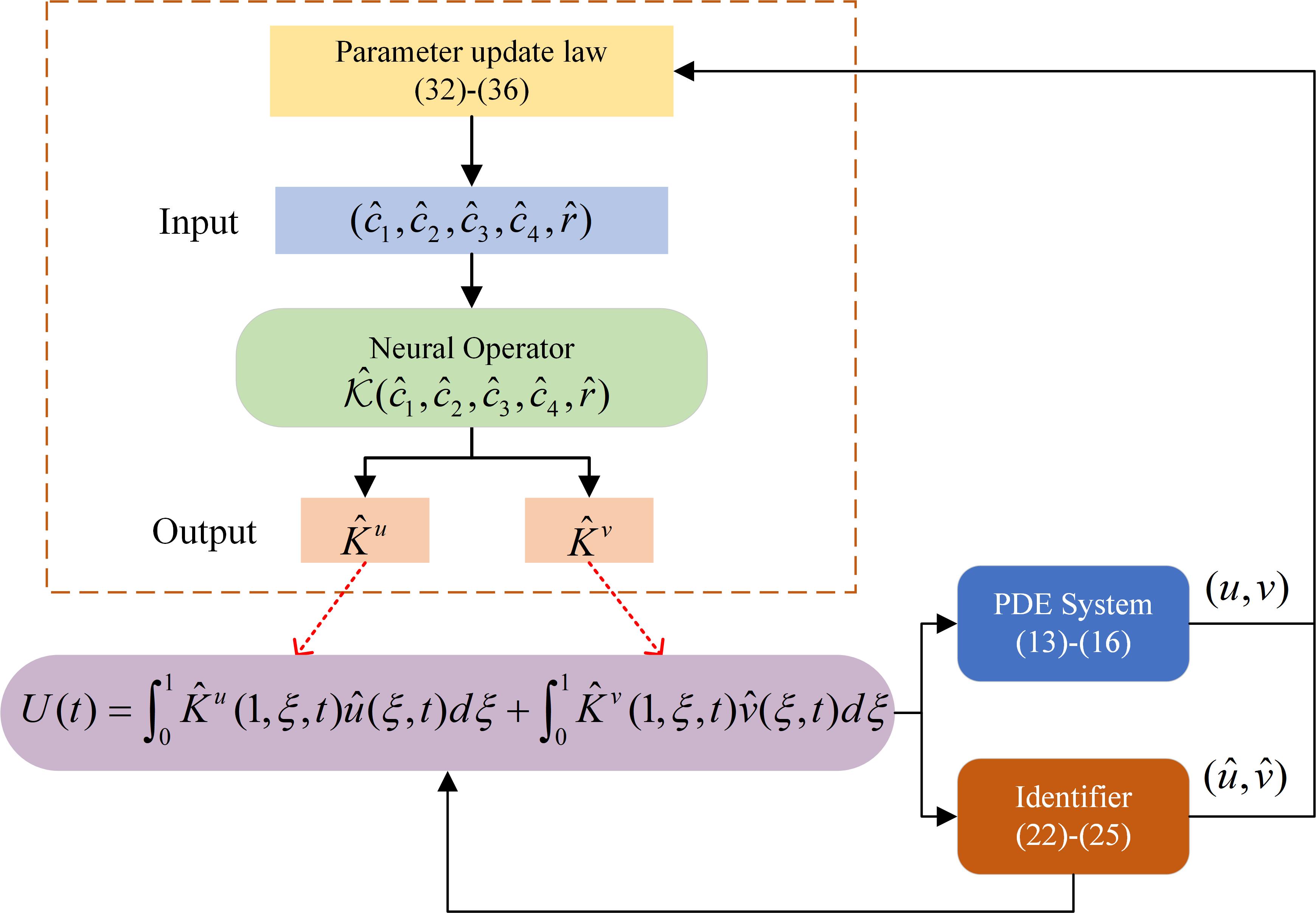
Figure 1: The NO learning framework for adaptive control.

Next, we define the operator $\mathcal{K}:(C^{0}([0,1]))^{4}\times\mathbb{R}\mapsto(C^{1}(\mathcal{T}))^{2}$

$$\mathcal{K}(\hat{c}_{1},\hat{c}_{2},\hat{c}_{3},\hat{c}_{4},\hat{r})(\cdot,t):=(\breve{K}^{u}(x,\xi),\breve{K}^{v}(x,\xi)).$$ (71)

Theorem 3.

[Existence of a NO to approximating the kernel] Consider the NO defined in (71), along with (2.2)-(53). Fixed $t>0$, Let $(\hat{c}_{1},\hat{c}_{2},\hat{c}_{3},\hat{c}_{4},\hat{r})\in\mathbb{R}\times C^{0}([0,1])$. Then for all $\mathcal{E}>0$ there exists a NO $\mathcal{\hat{K}}:\mathbb{R}^{3}\times(C^{0}([0,1]))^{4}\mapsto(C^{1}(\mathcal{T}))^{2}$ such that for all $\forall(x,\xi)\in\mathcal{T}$,

$$|\mathcal{K}(\hat{c}_{1},\hat{c}_{2},\hat{c}_{3},\hat{c}_{4},\hat{r})(\cdot,t)-\hat{\mathcal{K}}(\hat{c}_{1},\hat{c}_{2},\hat{c}_{3},\hat{c}_{4},\hat{r})(\cdot,t)|\leq\mathcal{E},$$

namely,

$$|\tilde{K}^{u}(\cdot,t)|+|\tilde{K}^{v}(\cdot,t)|\leq\mathcal{E}.$$ (72)

Proof.

The continuity of the operator $\mathcal{K}$ is derived from Lemma 2. And this result is based on Theorem 2.1 proposed by B. Deng et al. in their study [45]. ∎

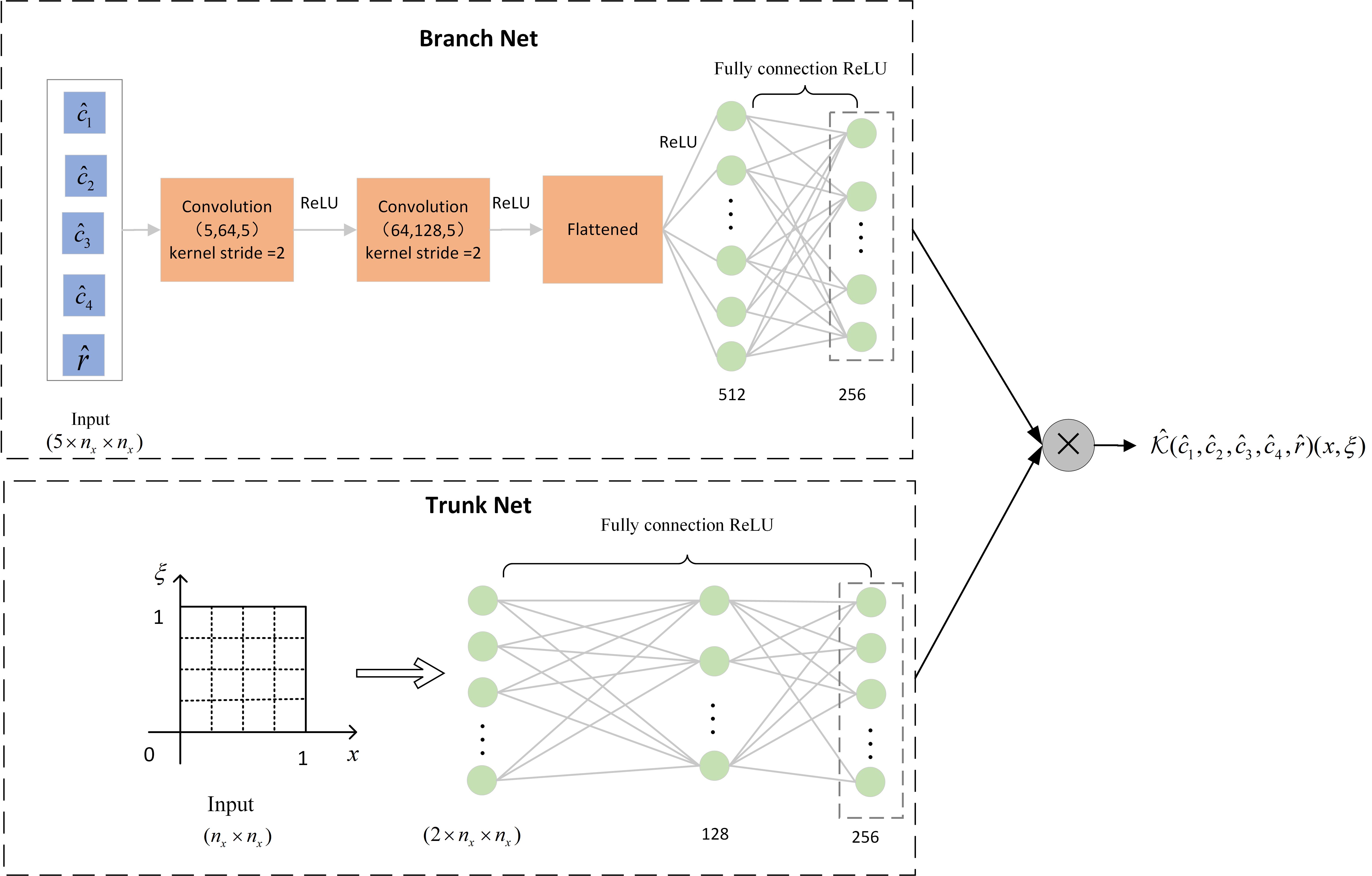
Figure 2: The DeepONet structure for operator $\hat{\mathcal{K}}$

4 Stabilization under DeepONet-Approximated Gain Feedback

We will demonstrate that although the adaptive controller uses approximate estimated kernel functions, the stability of the system is still guaranteed. Based on Theorem 1, we present the system stability proof for the adaptive backstepping controller using approximate estimation kernels $\hat{K}^{u},\hat{K}^{v}$ in the following theorem.

Theorem 4.

[Stabilization under approximate adaptive backstepping control] For all $\bar{c}_{1},\bar{c}_{2},\bar{c}_{3},\bar{c}_{4},\bar{r},\mathcal{E}>0$ there exists a $\mathcal{E}_{0}:=\frac{\sqrt{d}}{\sqrt{2\mu e^{k}}\bar{\Gamma}}$ such that for all NO approximations $\hat{K}^{u},\hat{K}^{v}$ of accuracy $\mathcal{E}\in(0,\mathcal{E}_{0})$ provided by Theorem 3, the plant (16)-(19) in feedback with the adaptive control law

$$U(t)=\int_{0}^{1}\hat{K}^{u}(1,\xi,t)\hat{u}(\xi,t)d\xi+\int_{0}^{1}\hat{K}^{v}(1,\xi,t)\hat{v}(\xi,t)d\xi,$$ (73)

along with the update law for $\hat{c}_{1},\hat{c}_{2},\hat{c}_{3},\hat{c}_{4}$ and $\hat{r}$ given by (35)-(39) with any Lipschitz initial condition $\hat{c}_{10}=\hat{c}_{1}(\cdot,0),\hat{c}_{20}=\hat{c}_{2}(\cdot,0),\hat{c}_{30}=\hat{c}_{3}(\cdot,0),\hat{c}_{40}=\hat{c}_{4}(\cdot,0),\hat{r}_{0}=\hat{r}(0)$ such that $\hat{c}_{10}\leq\bar{c}_{1},\hat{c}_{20}\leq\bar{c}_{2},\hat{c}_{30}\leq\bar{c}_{3},\hat{c}_{40}\leq\bar{c}_{4},\hat{r}_{10}\leq\bar{r}$ and the passive identifier $\hat{u}$, $\hat{v}$ given by (2.2)-(28) with any initial condition $\hat{u}_{0}=\hat{u}(\cdot,0),\hat{v}_{0}=\hat{v}(\cdot,0)$ such that $\|\hat{u}_{0}\|<\infty,\|\hat{v}_{0}\|<\infty$, the following properties hold:

$$\|u\|,\|v\|,\|\hat{u}\|,\|\hat{v}\|,\|{u}\|_{\infty},\|{v}\|_{\infty},\|\hat{u}\|_{\infty},\|\hat{v}\|_{\infty},\in L_{2}\cap L_{\infty},$$ (74)

$$\|{u}\|_{\infty},\|{v}\|_{\infty},\|\hat{u}\|_{\infty},\|\hat{v}\|_{\infty}\mapsto 0.$$ (75)

Moreover, for the equilibrium $(u,v,\hat{u},\hat{v},\hat{c}_{1},\hat{c}_{2},\hat{c}_{3},\hat{c}_{4},\hat{r})=(0,0,0,0,{c}_{1},{c}_{2},{c}_{3},{c}_{4},r)$ the following global stability estimate holds

$$S(t)\leq 2\dfrac{k_{2}}{k_{1}}\theta_{2}S(0)e^{\theta_{1}k_{2}S(0)},t>0,$$ (76)

where

$$S(t):= \|u\|^{2}+\|v\|^{2}+\|\hat{u}\|^{2}+\|\hat{v}\|^{2}+\|\tilde{c}_{1}\|^{2}+\|\tilde{c}_{2}\|^{2}$$

$$+\|\tilde{c}_{3}\|^{2}+\|\tilde{c}_{4}\|^{2}+\tilde{r}^{2},$$ (77)

and $k_{1}$, $k_{2}$, $\theta_{1}$ and $\theta_{2}$ are strictly positive constants.

Proof.

This proof mainly refers to [22, Chperter 9], and makes necessary supplements to the gain approximation error while reducing repetition.

Part A: DeepONet-perturbed target system

We consider the following adaptive backstepping transformation (48) and (49)

$$w(x,t)= \hat{u}(x,t),$$ (78)

$$z(x,t)= \hat{v}(x,t)-\int_{0}^{x}\breve{K}^{u}(x,\xi,t)\hat{u}(\xi,t)d\xi$$

$$-\int_{0}^{x}\breve{K}^{v}(x,\xi,t)\hat{v}(\xi,t)d\xi=T[\hat{u},\hat{v}](x,t),$$ (79)

where $\breve{K}^{u}$ and $\breve{K}^{v}$ are exact solutions to kernel function (2.2)-(53). The transformation is an invertible backstepping transformation, with inverse in the same form

$$\hat{u}(x,t)= w(x,t),$$ (80)

$$\hat{v}(x,t)= z(x,t)+\int_{0}^{x}\breve{L}^{u}w(\xi,t)d\xi$$

$$+\int_{0}^{x}\breve{L}^{v}z(\xi,t)d\xi=T^{-1}[w,z](x,t)$$ (81)

where $T^{-1}$ is an operator similar to $T$. According to [47], from Lemma 2, $K^{u},K^{v}$ are continuous, there exists a unique continuous inverse kernels $L^{u},L^{v}$ defined on $\mathcal{T}_{1}$ and there exits a constant $\bar{L}$ so that $\|\breve{L}^{u}\|_{\infty}\leq\bar{L}$, $\|\breve{L}^{v}\|_{\infty}\leq\bar{L}$. We will derive the DeepONet-perturbed target system with exact estimated kernels. Because the controller we have chosen is (73), where the kernels $\hat{K}^{u}$ and $\hat{K}^{v}$ are approximated by NO. This transformation lead to the following target system

$$w_{t}(x,t)= -\lambda w_{x}(x,t)+\hat{c}_{1}w(x,t)+\hat{c}_{1}e(x,t)+\hat{c}_{2}z(x,t)$$

$$+\int_{0}^{x}\omega(x,\xi,t)w(\xi,t)d\xi$$

$$+\int_{0}^{x}\kappa(x,\xi,t)z(\xi,t)d\xi$$

$$+\hat{c}_{2}\varepsilon(x,t)+\rho e(x,t)\|\varpi(t)\|^{2},$$ (82)

$$z_{t}(x,t)= \mu z_{x}(x,t)+\hat{c}_{4}z(x,t)-\lambda\breve{K}^{u}(x,0,t)r(t)\epsilon(0,t)$$

$$-\lambda\breve{K}^{u}(x,0,t)\tilde{r}(t)z(0,t)+\breve{K}^{u}(x,0,t)e(0,t)$$

$$-\int_{0}^{x}\breve{K}_{t}^{u}(x,\xi,t)w(\xi,t)d\xi$$

$$-\int_{0}^{x}\breve{K}_{t}^{v}(x,\xi,t)T^{-1}[w,z](\xi,t)d\xi$$

$$+T\left[\hat{c}_{1}e+\hat{c}_{2}\epsilon,\hat{c}_{3}e+\hat{c}_{4}\varepsilon\right](x,t)$$

$$+\rho T[e,\epsilon](x,t)\|\varpi(t)\|^{2},$$ (83)

$$w(0,t)= r(t)z(0,t)+r(t)\epsilon(0,t)-e(0,t),$$ (84)

$$z(1,t)= -\int_{0}^{1}\tilde{K}^{u}(1,\xi,t)w(\xi,t)d\xi$$

$$-\int_{0}^{1}\tilde{K}^{v}(1,\xi,t)T^{-1}[w,z](\xi,t)d\xi:=\Gamma(t),$$ (85)

where

$$\omega(x,\xi,t) =\hat{c}_{2}(x,t)\breve{K}^{u}(x,\xi,t)+\int_{\xi}^{x}\kappa(x,s,t)\breve{K}^{u}(s,\xi,t)ds,$$ (86)

$$\kappa(x,\xi,t) =\hat{c}_{2}(x,t)\breve{K}^{v}(x,\xi,t)+\int_{\xi}^{x}\kappa(x,s,t)\breve{K}^{v}(s,\xi,t)ds.$$ (87)

The main difference between the current system (82)-(85) and the system described in (55)-(58) is the perturbation $\Gamma(t)$ in the boundary conditions (85). This difference is due to the controller (73) using an approximated estimated kernels $\hat{K}^{u}$ and $\hat{K}^{v}$ instead of the exact estimated kernels $\breve{K}^{u}$ and $\breve{K}^{v}$. The specific derivation process of (85) is as follows

$$z(1,t)= \hat{v}(1,t)-\int_{0}^{1}\breve{K}^{u}(1,\xi,t)\hat{u}(\xi,t)d\xi$$

$$-\int_{0}^{1}\breve{K}^{v}(1,\xi,t)\hat{v}(\xi,t)d\xi$$

$$= U(t)-\int_{0}^{1}\breve{K}^{u}(1,\xi,t)\hat{u}(\xi,t)d\xi$$

$$-\int_{0}^{1}\breve{K}^{v}(1,\xi,t)\hat{v}(\xi,t)d\xi$$

$$= \int_{0}^{1}\hat{K}^{u}(1,\xi,t)\hat{u}(\xi,t)d\xi+\int_{0}^{1}\hat{K}^{v}(1,\xi,t)\hat{v}(\xi,t)d\xi$$

$$-\int_{0}^{1}\breve{K}^{u}(1,\xi,t)\hat{u}(\xi,t)d\xi-\int_{0}^{1}\breve{K}^{v}(1,\xi,t)\hat{v}(\xi,t)d\xi$$

$$= -\int_{0}^{1}\tilde{K}^{u}(1,\xi,t)\hat{u}(\xi,t)d\xi-\int_{0}^{1}\tilde{K}^{v}(1,\xi,t)\hat{v}(\xi,t)d\xi.$$

By using (81), we obtained (85).

Spatial $\mathcal{L}^{2}$ boundedness and regulation of plant and
observer states

We use the following Lyapunov function candidate

$$V(t):=V_{4}(t)+aV_{5}(t),$$ (88)

where $a>0$ and

$$V_{4}(t) :=\|w(t)\|_{-\delta}^{2}=\int_{0}^{1}e^{-\delta x}w^{2}(x,t)dx,$$ (89)

$$V_{5}(t) :=\|z(t)\|_{k}^{2}=\int_{0}^{1}e^{kx}z^{2}(x,t)dx.$$ (90)

Before we start the formal calculations of the Lyapunov function, we will present the inequalities derived from Lemma 1.

$$\|\breve{K}^{u}\|_{\infty}\leq\bar{K},\|\breve{K}^{v}\|_{\infty}\leq\bar{K},$$ (91)

$$\|\tilde{K}^{u}\|_{\infty}\leq\mathcal{E},\|\tilde{K}^{v}\|_{\infty}\leq\mathcal{E},$$ (92)

$$\|w(t)\|=\|\hat{u}(t)\|,$$ (93)

$$\|z(t)\|\leq(1+\bar{K}^{v})\|\hat{v}(t)\|+\bar{K}^{u}\|\hat{u}(t)\|,$$ (94)

$$\|\hat{v}(t)\|\leq(1+\bar{L})\|z(t)\|+\bar{L}\|w(t)\|,$$ (95)

$$\Gamma(t)\leq\mathcal{E}\bar{\Gamma}(\|w\|+\|z\|),$$ (96)

where

$$\bar{\Gamma}=1+\bar{L}.$$

The current work is based on the previous work [22, Chapter 9], with a key difference being that $z^{2}(1,t)=\Gamma(t)^{2}\neq 0$. This leads to the terms $2\mu e^{k}\mathcal{E}^{2}\bar{\Gamma}^{2}V(t)$ in (98) as follows. Let $\delta\geq 1$. There exist positive constants $h_{1},h_{2},\cdots,h_{6}$ and nonnegative, integrable function $l_{1},l_{2},\cdots,l_{5}$ such that

$$\dot{V}_{4}(t)\leq h_{1}w^{2}(0,t)-\left[\lambda\delta-h_{2}\right]V_{4}(t)+h_{3}V_{5}(t)$$

$$+l_{1}(t)V_{4}(t)+l_{2}(t),$$ (97)

$$\dot{V}_{5}(t)\leq -\left[\mu-e^{k}h_{4}\tilde{q}^{2}(t)\right]w^{2}(0,t)+h_{5}V_{4}(t)$$

$$-\left[k\mu-h_{6}\right]V_{5}(t)+l_{3}(t)V_{4}(t)+l_{4}(t)V_{5}(t)$$

$$+l_{5}(t)+2\mu e^{k}\mathcal{E}^{2}\bar{\Gamma}^{2}V(t).$$ (98)

Thus, we obtain the following upper bound calculation

$$\dot{V}(t)\leq-\left[d-2\mu e^{k}\mathcal{E}^{2}\bar{\Gamma}^{2}\right]V(t)+l_{6}(t)V(t)+l_{10}(t),$$ (99)

for positive constant $d$ and the nonnegative, integrable functions $l_{10}(t)$ and $l_{6}(t)$

$$l_{10}(t)= \dfrac{2\tilde{r}^{2}z(0,t)^{2}}{1+v(0,t)^{2}}+8b\tilde{r}^{2}\epsilon(0,t)^{2}+l_{2}(t)+al_{5}(t)$$

$$+b\dfrac{\tilde{r}^{2}z(0,t)^{2}}{1+v(0,t)^{2}}z(0,t)^{2},$$ (100)

$$l_{2}(t)= \left(\bar{c}_{1}^{2}+4e^{-\delta}\right)\|e(t)\|^{2}+\left(\bar{c}_{2}^{2}+4e^{-\delta}\right)\|\epsilon(t)\|^{2}$$

$$+3\lambda e^{2}(0,t)+3\lambda\bar{r}^{2}\epsilon^{2}(0,t),$$ (101)

$$l_{5}(t)= \lambda^{2}\bar{K}^{2}\bar{r}^{2}e^{k}\epsilon^{2}(0,t)+\lambda^{2}\bar{K}^{2}e^{k}e^{2}(0,t)$$

$$+2e^{k}A_{1}^{2}\bar{c}_{1}^{2}\|e(t)\|^{2}+2e^{k}A_{1}^{2}\bar{c}_{2}^{2}\|\epsilon(t)\|^{2}$$

$$+2e^{k}A_{2}^{2}\bar{c}_{3}^{2}\|e(t)\|^{2}+2e^{k}A_{2}^{2}\bar{c}_{4}^{2}\|\epsilon(t)\|^{2}$$

$$+4e^{-\delta}\|e(t)\|^{2}+4e^{-\delta}\|\epsilon(t)\|^{2},$$ (102)

$$l_{6}(t)= \mathop{\max}\left\{l_{1}(t)+al_{3}(t),l_{4}(t)\right\},$$ (103)

$$l_{1}(t)= e^{2\delta}\rho^{2}\|e(t)\|^{2}\|\varpi(t)\|^{2},$$ (104)

$$l_{3}(t)= e^{\delta+k}\left\|\hat{K}_{t}^{u}(t)\right\|^{2}+2e^{\delta+k}\left\|\hat{K}_{t}^{v}(t)\right\|^{2}A_{3}^{2},$$ (105)

$$l_{4}(t)= 2\rho^{2}e^{\delta+2k}\left(A_{1}^{2}\|e(t)\|^{2}+A_{2}^{2}\|\epsilon(t)\|^{2}\right)\|\varpi(t)\|^{2}$$

$$+2e^{k}\left\|\hat{K}_{t}^{v}(t)\right\|^{2}A_{4}^{2},$$ (106)

where $a,b,k,A_{i}$, $i=1\cdots 4$ are positive constants. We introduce

$$\mathcal{E}_{0}:=\dfrac{\sqrt{d}}{\sqrt{2\mu e^{k}}\bar{\Gamma}}.$$ (107)

Thus, if we choose $\mathcal{E}\in(0,\mathcal{E}_{0})$ we have $d-2\mu e^{k}\mathcal{E}^{2}\bar{\Gamma}^{2}>\frac{1}{2}>0$. It then follows from Lemma B.6 in [48] that

$$V\in\mathcal{L}_{1}\cap\mathcal{L}_{\infty},$$

and hence

$$\|u\|,\|v\|\in\mathcal{L}_{2}\cap\mathcal{L}_{\infty}.$$

Due to the invertibility of the backstepping transformation

$$\|\hat{u}\|,\|\hat{v}\|\in\mathcal{L}_{2}\cap\mathcal{L}_{\infty}.$$

From Lemma 1 it follows that

$$\|u\|,\|v\|\in\mathcal{L}_{2}\cap\mathcal{L}_{\infty}.$$

Part B: Pointwise-in-space boundedness and regulation

The paper [49] proved that the system (16)-(19) is equivalent to the following system through an invertible backstepping transformation.

$$\alpha_{t}(x,t) =-\lambda\alpha_{x}(x,t)+g(x)\beta(0,t),$$ (108)

$$\beta_{t}(x,t) =\mu\beta_{x}(x,t),$$ (109)

$$\alpha(0,t) =r\beta(0,t),$$ (110)

$$\beta(1,t) =U(t)-\int_{0}^{1}G_{1}(\xi)u(\xi)d\xi-\int_{0}^{1}G_{2}(\xi)v(\xi)d\xi,$$ (111)

for some bounded functions $g,G_{1},G_{2}\in\mathcal{C}$ fo the unknown parameters. Equation (108)-(111) can be explicitly be solved for $t>\lambda^{-1}+\mu^{-1}$ to yield

$$\alpha(x,t)= r\beta\left(1,t-\mu^{-1}-\lambda^{-1}x\right)$$

$$+\lambda^{-1}\int_{0}^{x}h(\tau)\beta\left(1,t-\mu^{-1}-\lambda^{-1}(x-\tau)\right)d\tau,$$ (112)

$$\beta(x,t)= \beta\left(1,t-\mu^{-1}(1-x)\right).$$ (113)

From (111), the control law $U(t)$ and $\|u\|,\|v\|,\|\hat{u}\|,\|\hat{v}\|\in$ $\mathcal{L}_{2}\cap\mathcal{L}_{\infty}$, it follows that $\beta(1,\cdot)\in$ $\mathcal{L}_{2}\cap\mathcal{L}_{\infty}$. Since $\beta$ and $\alpha$ are simple, cascaded transport equations, this implies

$$\|\alpha\|_{\infty},\|\beta\|_{\infty}\in\mathcal{L}_{2}\cap\mathcal{L}_{\infty},\quad\|\alpha\|_{\infty},\|\beta\|_{\infty}\rightarrow 0.$$ (114)

With the invertibility of the transformation, then yields

$$\|u\|_{\infty},\|v\|_{\infty}\in\mathcal{L}_{2}\cap\mathcal{L}_{\infty},\quad\|u\|_{\infty},\|v\|_{\infty}\rightarrow 0.$$ (115)

From the structure of the identifier (16), we will also have $\hat{u}(x,\cdot),\hat{v}(x,\cdot)\in\mathcal{L}_{\infty}\cap\mathcal{L}_{2}$ , and hence

$$\|\hat{u}\|_{\infty},\|\hat{v}\|_{\infty}\in\mathcal{L}_{\infty}\cap\mathcal{L}_{2},\quad\|\hat{u}\|_{\infty},\|\hat{v}\|_{\infty}\mapsto 0.$$ (116)

Part C: Global stability

Here, we will prove the global stability of the system, specifically by proving (76), and thus we introduce the following function

$$S(t):= \|u\|^{2}+\|v\|^{2}+\|\hat{u}\|^{2}+\|\hat{v}\|^{2}+\|\tilde{c}_{1}\|^{2}+\|\tilde{c}_{2}\|^{2}$$ (117)

$$+\|\tilde{c}_{3}\|^{2}+\|\tilde{c}_{4}\|^{2}+\tilde{r}^{2}.$$ (118)

The goal of the proof is to demonstrate the existence of a function $\theta\in\mathcal{K}_{\infty}$ such that the following inequality holds.

$$S(t)\leq\theta(S(0)),t\geq 0.$$ (119)

We will reuse the Lyapunov function from Appendix to show that the system’s state remains stable over time.

$$V_{1}(t)= V_{2}(t)+\gamma_{1}^{-1}\|\tilde{c}_{1}\|^{2}+\gamma_{2}^{-1}\|\tilde{c}_{2}\|^{2}+\gamma_{3}^{-1}\|\tilde{c}_{3}\|^{2}$$

$$+\gamma_{4}^{-1}\|\tilde{c}_{4}\|^{2}+\dfrac{1}{2\gamma_{5}}\tilde{r}^{2}(t),$$ (120)

where

$$V_{2}(t)=\int_{0}^{1}e^{-\gamma x}e^{2}(x,t)dx+\int_{0}^{1}e^{\gamma x}\varepsilon^{2}(x,t)dx,$$ (121)

leads to the following upper bound:

$$\dot{V}_{1}(t)\leq -\lambda e^{-\gamma}e^{2}(1,t)-\lambda e^{2}(0,t)v^{2}(0,t)-\lambda\gamma e^{-\gamma}\|e(t)\|^{2}$$

$$-2\rho e^{-\gamma}\|e(t)\|^{2}\|\varpi(t)\|^{2}-\mu\epsilon^{2}(0,t)$$

$$-\mu\gamma\|\epsilon(t)\|^{2}-2\rho e^{\gamma}\|\epsilon(t)\|^{2}\|\varpi(t)\|^{2},$$ (122)

which shows that ${V}_{1}(t)$ is non-increasing and hence bounded. Thus implies that the ${V}_{1}(t)<V_{1}(0)$ and limit $\lim_{t\to\infty}V_{1}(t)=V_{1,\infty}$ exists. By integrating (122) from zero to infinity, we obtain the following upper bound:

$$\lambda e^{-\gamma}\int_{0}^{\infty}e^{2}(1,\tau)d\tau+\lambda\int_{0}^{\infty}e^{2}(0,\tau)v^{2}(0,\tau)d\tau$$

$$+\lambda\gamma e^{-\gamma}\int_{0}^{\infty}\|e(\tau)\|^{2}d\tau$$

$$+2\rho e^{-\gamma}\int_{0}^{\infty}\|e(\tau)\|^{2}\|\varpi(\tau)\|^{2}d\tau+\mu\int_{0}^{\infty}\epsilon^{2}(0,\tau)d\tau$$

$$+\mu\gamma\int_{0}^{\infty}\|\epsilon(\tau)\|^{2}d\tau+2\rho e^{\gamma}\int_{0}^{\infty}\|\epsilon(\tau)\|^{2}\|\varpi(\tau)\|^{2}d\tau$$

$$\leq V_{1}(0).$$ (123)

From (100) and (103), it can be concluded that there are constants $\theta_{1}>0$ and $\theta_{2}>1$ such that

$$\|l_{6}\|_{1}\leq \theta_{1}V_{1}(0),$$ (124)

$$\|l_{10}\|_{1}\leq \theta_{2}V_{1}(0).$$ (125)

Recalling (99), we have that

$$\dot{V}(t)\leq-\frac{1}{2}V(t)+l_{6}(t)V(t)+l_{10}(t).$$ (126)

We also have from Lemma B.6 in [48] that

$$V(t)\leq(e^{-\frac{1}{2}t}V(0)+\|l_{10}\|_{1})e^{\|l_{6}\|_{1}}.$$ (127)

We then introduce the function

$$V_{3}(t):=V_{1}(t)+V(t).$$ (128)

Noticing that

$$V_{1}(t)\leq V_{1}(0)\leq\theta_{2}V_{1}(0)e^{\theta_{1}V_{1}(0)},$$ (129)

we achieve from (127), (129), (124) and (125) the following

$$V_{3}(t)= V(t)+V_{1}(t)$$

$$\leq (e^{-\frac{1}{2}t}V(0)+\|l_{10}\|_{1})e^{\|l_{6}\|_{1}}+\theta_{2}V_{1}(0)e^{\theta_{1}V_{1}(0)}$$

$$\leq (\theta_{2}V(0)+\theta_{2}V_{1}(0))e^{\|l_{6}\|_{1}}+\theta_{2}V_{1}(0)e^{\theta_{1}V_{1}(0)}$$

$$\leq 2\theta_{2}V_{3}(0)e^{\theta_{1}V_{3}(0)}.$$ (130)

This Lyapunov functional can be represented by an equivalent norm, and the bounds of this equivalent norm are determined by two positive constants $k_{1}>0$ and $k_{2}>0$.

$$k_{1}S(t)\leq V_{3}(t)\leq k_{2}S(t).$$ (131)

So we have

$$S(t)\leq 2\dfrac{k_{2}}{k_{1}}\theta_{2}S(0)e^{\theta_{1}k_{2}S(0)}.$$ (132)

∎

5 Simulations

This section will present and analyze the performance of the proposed NO-based adaptive controllers for two PDE models: (i) a general 2$\times$2 hyperbolic system (16)-(19) (ii) the ARZ PDE system. Through these examples, we will demonstrate the effectiveness of the NO-based adaptive control design.

5.1 Simulation of the Coupled 2$\times$2 Hyperbolic System

A. Simulation configuration

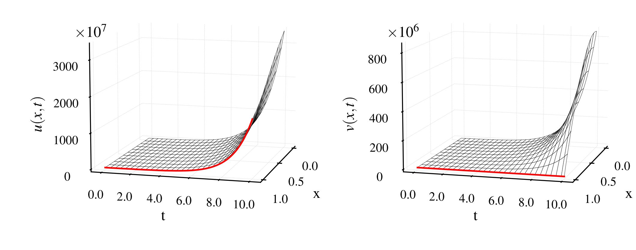
Figure 3: Open-loop $u(x,t)$ and $v(x,t)$. We note that the plant is open-loop unstable.

The coefficients of system (16)-(19) are defined as $c_{1}(x)=\cos(\sigma_{1}\cos^{-1}(x))$, $c_{2}(x)=\cos(\sigma_{2}\cos^{-1}(x))$, $c_{3}(x)=\sin(1-\sigma_{3}x)+1$ and $c_{4}(x)=\cos(\sigma_{4}x)$ with the shape parameters $\sigma_{1}$, $\sigma_{2}$, $\sigma_{3}$ and $\sigma_{4}$. We choose the spatially varying coefficient from three classes of functions—namely the Chebyshev polynomial forms, sine function and cosine function. Because these coefficients are both bounded and equicontinuous, satisfying the compactness requirement of Theorem 3. And We can generate a rich and diverse set of kernel functions for training data by varying a single parameter $\sigma_{1}$, $\sigma_{2}$, $\sigma_{3}$ and $\sigma_{4}$. Although this paper uses specific Chebyshev polynomial forms, sine functions, and cosine functions, our framework is applicable to any compact set of continuous functions. We use the finite difference scheme to solve PDEs, where the time step $dt=0.005s$, the spatial step $dx=0.05m$, the total time $T=10s$, and the length $L=1m$. The initial conditions are $u_{0}=\sin(2\pi x)$, $v_{0}=x$. We demonstrate in the Figure 3 that the system is open-loop unstable.

B. Dataset generation and NO training

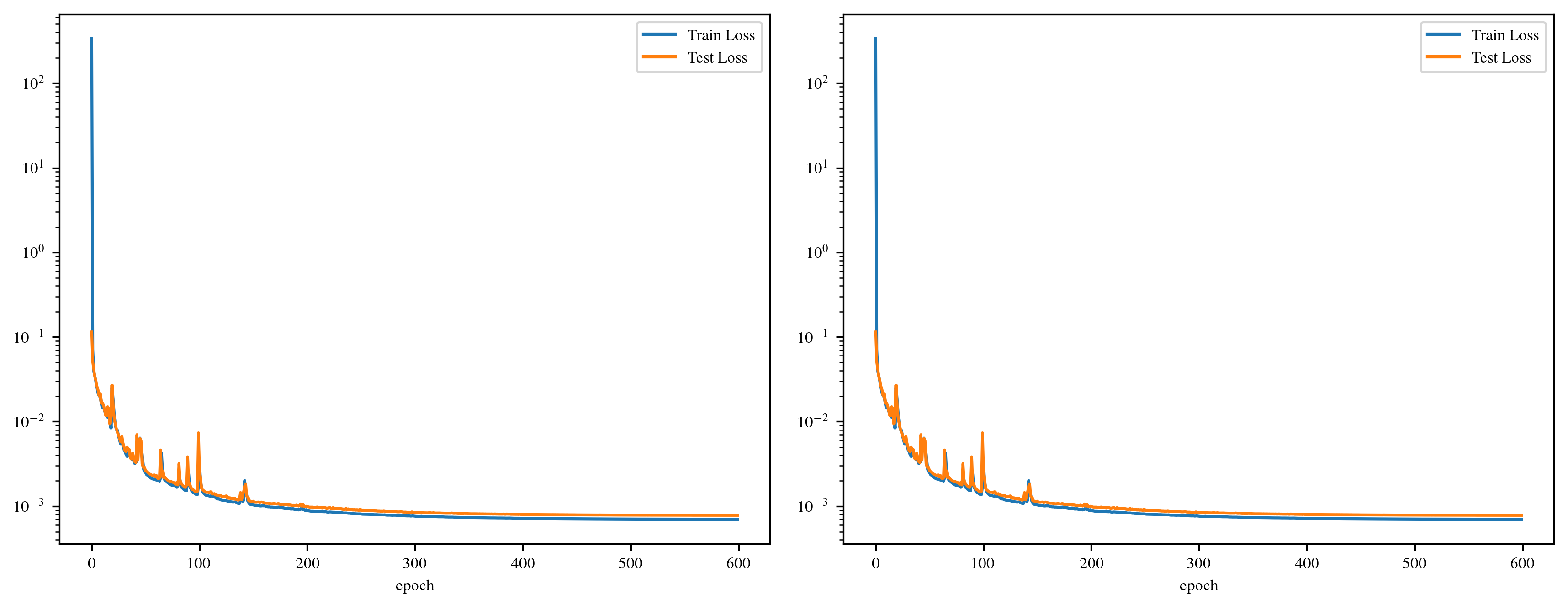
Figure 4: The train and test loss for $\breve{K}^{u}$ and $\breve{K}^{v}$

In order to establish a mapping $(\hat{c}_{1},\hat{c}_{2},\hat{c}_{3},\hat{c}_{4},\hat{r})\mapsto(\breve{K}^{u},\breve{K}^{v})$, one must build a sufficiently large dataset containing the $(\hat{c}_{1}(x),\hat{c}_{2}(x),\hat{c}_{3}(x),\hat{c}_{4}(x),\hat{r})$ values that may be encountered. In this work, we choose 10 sets of $(c_{1},c_{2},c_{3},c_{4},r)$ randomly sampled with $\sigma_{1}\sim U(3.5,4.5)$, $\sigma_{2}\sim U(0.8,1)$, $\sigma_{3}\sim U(20,21)$, $\sigma_{4}\sim U(10,11)$ and $r\sim U(2,5)$, where $U(a,b)$ denotes the uniform distribution over the interval $[a,b]$. We simulate trajectories using adaptive control methods and calculate the corresponding kernel functions using numerical solvers. Each trajectory was sampled at $1000$ time points, resulting in a dataset of $10000$ sets of $(\hat{c}_{1},\hat{c}_{2},\hat{c}_{3},\hat{c}_{4},\hat{r},\breve{K}^{u},\breve{K}^{v})$ for training. We trained the model on an Nvidia RTX 4060 Ti GPU. After 600 epochs of training, the $L_{2}$ error of kernel $\breve{K}^{u}$ reached $1.2\times 10^{-3}$, and the test error was $1.1\times 10^{-3}$. The $L_{2}$ error of kernel $\breve{K}^{v}$ reached $1.3\times 10^{-3}$, and the testing error was $1.2\times 10^{-3}$, as shown in Figure 4.

C. Computation time comparison

We begin to discuss the computational acceleration performance of NO. Table 2 provides a comparison of the computation time of solving kernels at each time step using the numerical solver and the trained DeepONet model. The last column of Table 2 represents the multiple of acceleration calculation. As the sampling accuracy increases (i.e.,the discrete space step size $dx$ decreases), the calculation time of the finite-difference method will significantly increase. In contrast, the calculation time of NO only slightly increases with the decrease of spatial step size. We can see that as the sampling accuracy improves, the acceleration obtained by the NO becomes substantial. Especially when the spatial step size dx=0.0005, the kernel computation time is shortened from 3.191s to 4.631 $\times 10^{-3}$s. We computed the average absolute error $\int_{\xi}^{1}\int_{0}^{x}(|\breve{K}^{u}-\hat{K}^{u}|+|\breve{K}^{v}-\hat{K}^{v}|)d\xi dx$ between numerical solutions and NO solutions with different step sizes. Although the error slightly increases with the decrease of step size, they are quite small at all step sizes. Because adaptive control requires calculating control gain at every step of updating parameter estimation, quickly solving the kernel function can help improve the performance of adaptive control.

D. Simulation results

We test the performance of the closed-loop system stability with test values $(\sigma_{1}=4,\sigma_{2}=0.9,\sigma_{3}=20.1,\sigma_{4}=10.1,r=4)$ unseen during training. Figure 5 shows the kernels $\breve{K}^{u},\breve{K}^{v}$ calculated by the numerical solver, the kernels $\hat{K}^{u},\hat{K}^{v}$ learned by DeepONet, and the error between them. In Figure 6, we demonstrate closed-loop stability with the NO approximated kernel function for the control feedback law. The NO approximation of the kernels is illustrated in Figure 5, where most of the absolute pointwise errors for the learned kernel do not exceed 0.03. Figure 5 and Figure 6 confirm that the kernels $\hat{K}^{u},\hat{K}^{v}$ approximated by NO can effectively simulate the backstepping kernels $\breve{K}^{u},\breve{K}^{v}$ while maintaining the stability of the system. All estimated parameters $\hat{c}_{i}$ and $\hat{r}$ are shown in Figure LABEL:coefficient_ci. We emphasize that although in adaptive control the system parameters $\hat{c}_{1},\hat{c}_{2},\hat{c}_{3},\hat{c}_{4}$ and $\hat{r}$ may not precisely converge to their true values, this does not affect the control performance. This phenomenon is not a problem but rather a characteristic of adaptive control. The goal of adaptive control is not perfect system identification, but rather the estimation of parameters that ensure system stability.

E. Comparative experiment with RL

We will evaluate the performance of NO-based (DeepONet) adaptive control method and RL method for stabilization results under different initial conditions. Specifically, we assume that the initial condition of state $u$ is a sine function, and the specific form is

$$u_{0}=\sin(\omega_{0}\pi x),$$ (133)

where $\omega_{0}$ is the frequency of a sine wave. To evaluate the performance of these two methods, we train DeepONet and RL at the same frequency $\omega_{0}=2$, ensuring all other parameters remained consistent with those in Figure 5. In the testing phase, we will use sine initial conditions of different frequencies $\omega_{0}=2,10$ to verify the model stability of NO-based adaptive control and RL. Figure LABEL:Comparison_with_RL shows the stabilization results of the RL and NO control under different initial conditions. The comparative experiments highlight a significant advantage of the NO-based adaptive control method, which consistently demonstrates robustness across different initial conditions. Specifically, the NO-based adaptive control method maintains system stability without requiring retraining even when the initial conditions are changed. This characteristic underscores its adaptability in dynamic environments. In contrast, the RL method shows a significant dependency on initial conditions. Although it performs well under specific conditions encountered during training, it is unstable when faced with unforeseen initial conditions($\omega_{0}=10$).In real-world scenarios where initial conditions are often variable and unpredictable, DeepONet ensures stability and adaptability without the need for retraining. In summary, this demonstrates DeepONet’s potential for more reliable applications in adaptive control systems, where maintaining performance across diverse conditions is crucial.

Spatial Step Size	Numerical solver (s)	NO(s)	Speedup	Error
dx=$0.01$	$8.221\times 10^{-3}$	$4.38\times 10^{-3}$	$2\times$	$0.024$
dx=$0.05$	$2.432\times 10^{-2}$	$4.42\times 10^{-3}$	$58\times$	$0.031$
dx=$0.001$	$8.701\times 10^{-1}$	$4.513\times 10^{-3}$	$192\times$	$0.037$
dx=$0.0005$	$3.191$	$4.631\times 10^{-3}$	$689\times$	$0.045$

Table 2: Comparison of computation time of kernels $\breve{K}^{u}$ and $\breve{K}^{v}$.

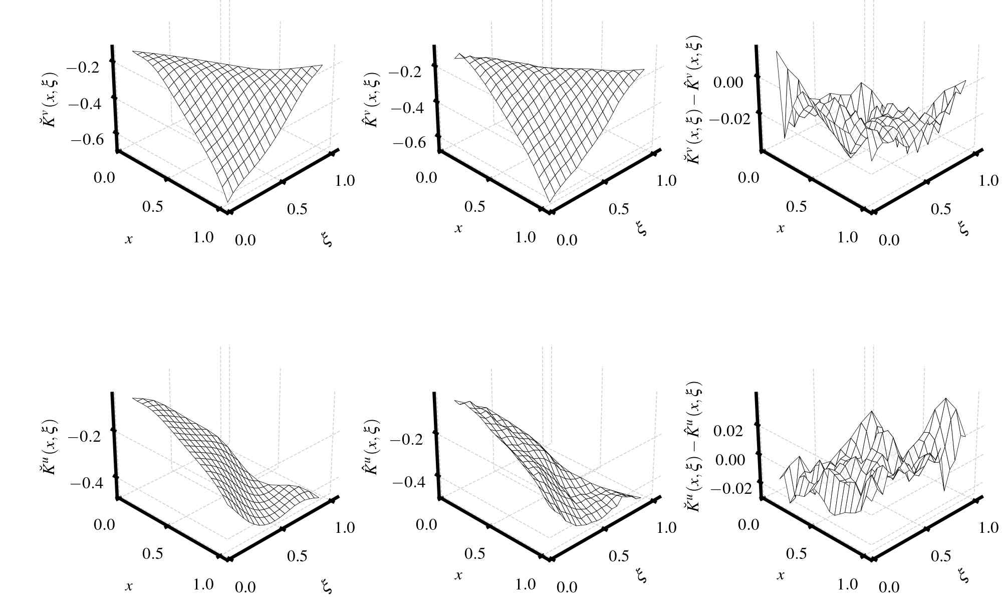
Figure 5: The first row shows the exact estimated kernels $\breve{K}^{u}$ and $\breve{K}^{v}$. The second row shows the NO estimated kernels $\hat{K}^{u}$ and $\hat{K}^{v}$. The last row shows the kernel errors $\breve{K}^{u}-\hat{K}^{u}$ and $\breve{K}^{v}-\hat{K}^{v}$. All kernels are plotted at the final time $T$.

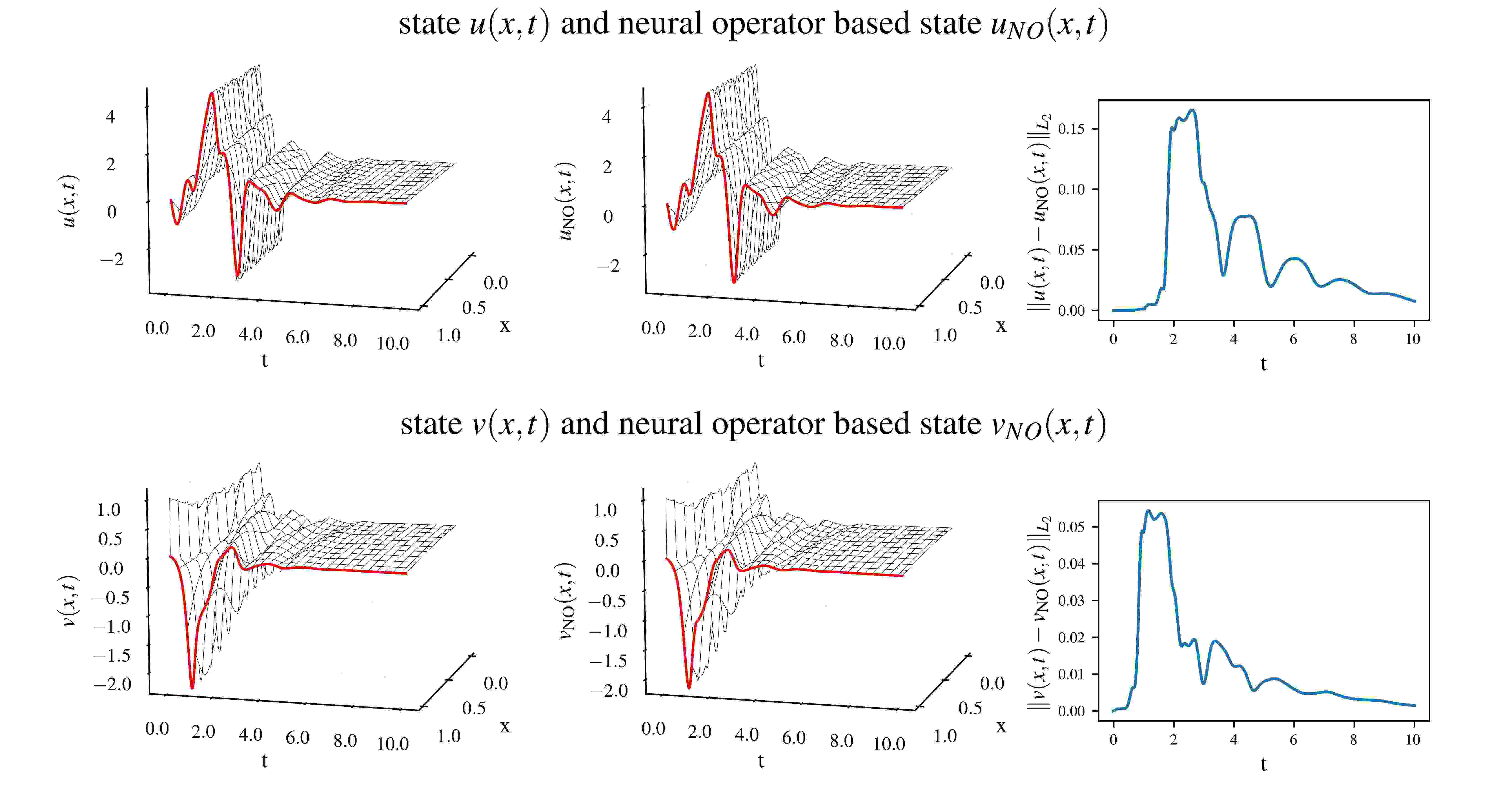
Figure 6: Simulation of the close-loop system with the update law (35)-(39), feedback controller (62) and (73). The left columns of the first and second rows show close-loop system states $u(x,t)$, $v(x,t)$ with the analyzed kernels $\breve{K}^{u}$ and $\breve{K}^{v}$. The middle columns of the first and second rows show close-loop system states $u_{NO}(x,t)$, $v_{NO}(x,t)$ with the approximated kernels $\hat{K}^{u}$ and $\hat{K}^{v}$. The right columns of the first and second rows show the errors between $u(x,t)$ and $u_{NO}(x,t)$, and between $v(x,t)$ and $v_{NO}(x,t)$, respectively.

5.2 Application Simulation of the ARZ Traffic System

A. NO-based adaptive controller

Following the steps in the section 2, we can obtain the adaptive controller for ARZ traffic system (5)-(8) as follows

$$U(t)=\int_{0}^{1}\breve{K}^{u_{1}}(1,\xi,t)\tilde{u}_{1}(\xi,t)d\xi+\int_{0}^{1}\breve{K}^{v_{1}}(1,\xi,t)\tilde{v}_{1}(\xi,t)d\xi,$$ (134)

with the parameter update law

$$\hat{c}_{t}(x,t)=\operatorname{Proj}_{\bar{c}}\left\{\gamma_{3}e^{\gamma x}\varepsilon_{1}(x,t){\tilde{u}_{1}}(x,t),\hat{c}(x,t)\right\},$$ (135)

where

$$\epsilon_{1}(x,t)=v_{1}(x,t)-\hat{v}_{1}(x,t),$$ (136)

and the kernels satisfy the following kernel functions

$$(\gamma p^{\star}-{v_{1}}^{\star})\breve{K}_{x}^{u_{1}}(x,\xi,t)= {v_{1}}^{\star}\breve{K}_{\xi}^{u_{1}}(x,\xi,t)$$

$$+\hat{c}(x,t)\breve{K}^{v_{1}}(x,\xi,t),$$ (137)

$$(\gamma p^{\star}-{v_{1}}^{\star})\breve{K}_{x}^{v_{1}}(x,\xi,t)= -(\gamma p^{\star}-{v_{1}}^{\star})\breve{K}_{\xi}^{v_{1}}(x,\xi,t),$$ (138)

$$\breve{K}^{u_{1}}(x,x,t)= -\frac{\hat{c}(x,t)}{\gamma p^{\star}},$$ (139)

$$\breve{K}^{v_{1}}(x,0,t)= \dfrac{{v_{1}}^{\star}}{\gamma p^{\star}-{v_{1}}^{\star}}r\breve{K}^{u_{1}}(x,0,t).$$ (140)

According to the approximation of NO in Theorem 3, we get the NO-based adaptive controller

$$U(t)=\int_{0}^{1}\hat{K}^{u_{1}}(1,\xi,t)\tilde{u}_{1}(\xi,t)d\xi+\int_{0}^{1}\hat{K}^{v_{1}}(1,\xi,t)\tilde{v}_{1}(\xi,t)d\xi.$$ (141)

Method	Average Computation Time (s)	Error
Nominal Adaptive Controller	$1.92$	$0$
NO-based adaptive Controller	$0.036$	$0.032$

Table 3: The computation time and error of nominal adaptive controller and NO-based adaptive controller.

B. Simulation results

Then, we analyze the performance of the proposed NO-based adaptive control law for the ARZ traffic PDE system through simulations on a L=600m road over T=300 seconds. The parameters are set as follows: free-flow velocity $v_{m}=40$ m/s, maximum density $\rho_{m}=160$ veh/km, equilibrium density $\rho_{1}^{\star}=120$ veh/km, driver reaction time $\tau=60$ s. Let $\gamma_{0}=1$. Initial conditions are sinusoidal inputs $\rho_{1}(x,0)=\rho_{1}^{\star}+0.1\sin(\frac{3\pi x}{L})\rho_{1}^{\star}$ and $v_{1}(x,0)=v_{1}^{\star}-0.01\sin(\frac{3\pi x}{L})v^{\star}$ to mimic stop-and-go traffic. To generate a sufficient dataset for training, we use 10 different $c(x)$ functions with $\tau\in U[50,70]$ and simulate the resulting PDEs under the adaptive controller for $T=300$ seconds. We sub-sample each $(c,\hat{K}^{u_{1}},\hat{K}^{v_{1}})$ pair every 0.1 seconds, resulting in a total of 30,000 distinct $(c,\hat{K}^{u_{1}},\hat{K}^{v_{1}})$ pairs for training the NO. Using the trained NO, we simulate with the same parameters. Figure 11 shows the ARZ system is open-loop unstable. Figures LABEL:rho_v show the density and velocity of ARZ traffic system with the adaptive controller (134) with the update law (135) and NO-based adaptive controller (141). The blue line indicates the initial condition, whereas the red line represents the boundary condition of the system. The results indicate that both the NO-based adaptive method and the adaptive backstepping control method effectively stabilize the transportation system. The traffic density and velocity converge to the equilibrium values of $\rho_{1}^{\star}=120$ veh/km and $v_{1}^{\star}=36$ m/s, respectively. The relative $L_{2}$ error between the closed-loop states of the nominal adaptive controller and the NO-based adaptive controller is shown in Figures LABEL:rho_v. The maximum error does not exceed 10$\%$. The estimated parameter $\hat{c}$ is shown in Figure 17.

Table 3 presents the computation times for both the nominal adaptive controller and the NO-based adaptive controller. As the baseline result, the nominal adaptive control method is compared with the NO-based adaptive control method. Notably, the NO-based adaptive control method not only achieves significantly faster average computation times but also maintains superior accuracy with a lower relative $L_{2}$ error. These advantages of the NO-based adaptive control method not only enhance computational efficiency but also make it highly suitable for real-time traffic system applications. The NO method’s efficiency and accuracy represent a substantial advancement, promising more effective and scalable traffic control strategies in practical scenarios.

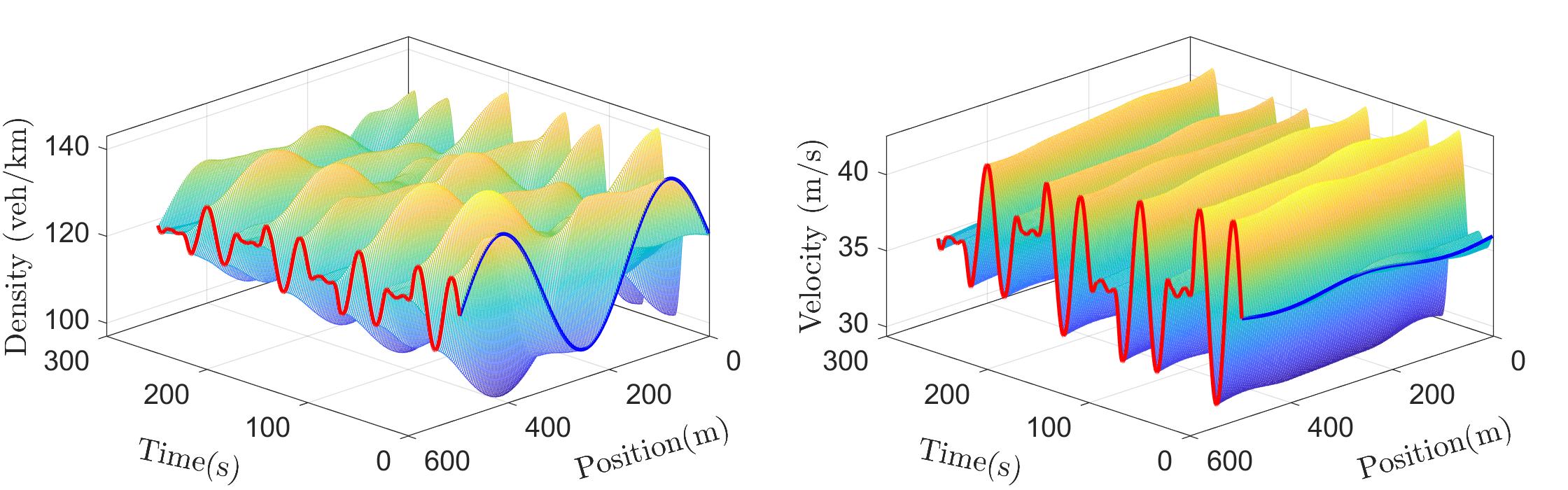
Figure 11: Density and velocity evolution of open-loop ARZ traffic system

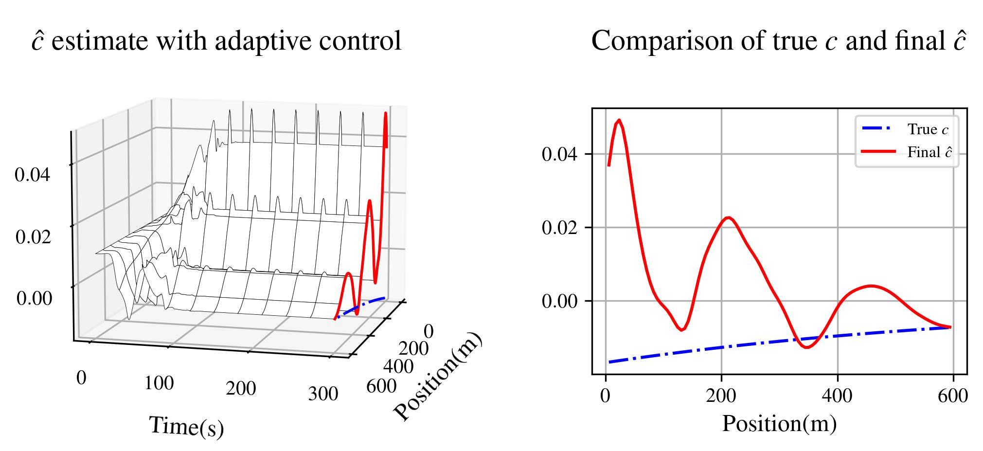
Figure 17: Parameter estimation of $\hat{c}$ in ARZ traffic system and comparision of true $c$ and $\hat{c}$

6 Conclusion

This paper builds upon prior studies such as [42] and [43], which primarily focused on approximating a single kernel PDE. In contrast, our work accelerates the computation of 2$\times$2 coupled Goursat-form PDEs that arise from the application of adaptive control designs to a 2$\times$2 linear first-order hyperbolic system. In this paper, the DeepONet is used to learn the adaptive control gains for stabilizing the traffic PDE system, and it is shown that under the DeepONet-approximated kernels the stabilization of 2$\times$2 hyperbolic PDEs can still be achieved with significant improvement for computational speeds. Experimental results show that compared to traditional numerical solvers, our method improves computational efficiency by two orders of magnitude. Additionally, compared with RL, the NO-based adaptive control strategy is independent of the system’s initial conditions, making it more robust for rapidly changing traffic scenarios. Our method significantly accelerates the process of obtaining adaptive controllers in PDE systems, greatly improving the real-time applicability of adaptive control strategies for mitigating traffic congestion. In the future, we will incorporate real traffic data into the training of the neural operator.

Appendix

The proof of Lemma 1.

Property (42) follows trivially from projection in (35)-(38) and Lemma A.1 in [22]. The result can be easily obtained using the following Lyapunov function candidate:

$$V_{1}(t)= V_{2}(t)+\gamma_{1}^{-1}\|\tilde{c}_{1}\|^{2}+\gamma_{2}^{-1}\|\tilde{c}_{2}\|^{2}+\gamma_{3}^{-1}\|\tilde{c}_{3}\|^{2}$$

$$+\gamma_{4}^{-1}\|\tilde{c}_{4}\|^{2}+\dfrac{1}{2}\gamma_{5}^{-1}\tilde{r}^{2}(t),$$ (142)

where

$$V_{2}(t)=\int_{0}^{1}e^{-\gamma x}e^{2}(x,t)dx+\int_{0}^{1}\varepsilon^{\gamma x}e^{2}(x,t)dx.$$ (143)

Computing the time derivative of (142) along (31)-(34) as

$$\dot{V}_{1}(t)= 2\int_{0}^{1}e^{-\gamma x}e(x,t)e_{t}(x,t)+e^{\gamma x}\varepsilon(x,t)\varepsilon_{t}(x,t)dx$$

$$+2\gamma_{1}^{-1}\int_{0}^{1}\tilde{c}_{1}(x,t)\tilde{c}_{1t}(x,t)dx$$

$$+2\gamma_{2}^{-1}\int_{0}^{1}\tilde{c}_{2}(x,t)\tilde{c}_{2t}(x,t)dx$$

$$+2\gamma_{3}^{-1}\int_{0}^{1}\tilde{c}_{3}(x,t)\tilde{c}_{3t}(x,t)dx$$

$$+2\gamma_{4}^{-1}\int_{0}^{1}\tilde{c}_{4}(x,t)\tilde{c}_{4t}(x,t)dx+\lambda\gamma_{5}^{-1}\tilde{r}(t)\dot{\tilde{r}}(t).$$ (144)

We put into the dynamics (31)-(34), integrating by parts, thus we have

$$\dot{V}_{1}(t)= -\lambda e^{-\gamma}e^{2}(1,t)+\lambda e^{2}(0,t)-\lambda\gamma\int_{0}^{1}e^{-\gamma x}e^{2}(x,t)dx$$

$$+2\int_{0}^{1}e^{-\gamma x}e(x,t)\varpi^{T}(x,t)\tilde{c}_{1}(x,t)dx$$

$$-2\rho\int_{0}^{1}e^{-\gamma x}e^{2}(x,t)\|\varpi(t)\|^{2}dx$$

$$-\mu\epsilon^{2}(0,t)-\mu\gamma\int_{0}^{1}e^{\gamma x}\epsilon^{2}(x,t)dx$$

$$+2\int_{0}^{1}e^{\gamma x}\epsilon(x,t)\varpi^{T}(x,t)\tilde{c}_{2}(x,t)dx$$

$$-2\rho\int_{0}^{1}e^{\gamma x}\epsilon^{2}(x,t)\|\varpi(t)\|^{2}dx$$

$$+2\gamma_{1}^{-1}\int_{0}^{1}\tilde{c}_{1}(x,t)\tilde{c}_{1t}(x,t)dx$$

$$+2\gamma_{2}^{-1}\int_{0}^{1}\tilde{c}_{2}(x,t)\tilde{c}_{2t}(x,t)dx$$

$$+2\gamma_{3}^{-1}\int_{0}^{1}\tilde{c}_{3}(x,t)\tilde{c}_{3t}(x,t)dx$$

$$+2\gamma_{4}^{-1}\int_{0}^{1}\tilde{c}_{4}(x,t)\tilde{c}_{4t}(x,t)dx+\lambda\gamma_{5}^{-1}\tilde{r}(t)\dot{\tilde{r}}(t).$$ (145)

Inserting the adaptive laws (35)-(39), and using the property (40), give

$$\begin{split}\dot{V}_{1}(t)\leq&-\lambda e^{-\gamma}e^{2}(1,t)+\lambda e^{2}(0,t)-\lambda\gamma\int_{0}^{1}e^{-\gamma x}e^{2}(x,t)dx\\ &-2\rho\int_{0}^{1}e^{-\gamma x}e^{2}(x,t)\|\varpi(t)\|^{2}dx\\ &-\mu\epsilon^{2}(0,t)-\mu\gamma\int_{0}^{1}e^{\gamma x}\epsilon^{2}(x,t)dx\\ &-2\rho\int_{0}^{1}e^{\gamma x}\epsilon^{2}(x,t)\|\varpi(t)\|^{2}dx-\lambda\tilde{r}(t)e(0,t)v(0,t).\end{split}$$ (146)

From the boundary condition (33), we have

$$e(0,t)=\tilde{r}(t)v(0,t)-e(0,t)v^{2}(0,t),$$ (147)

By substituting this, we obtain

$$\dot{V}_{1}(t)\leq -\lambda e^{-\gamma}e^{2}(1,t)-\lambda e^{2}(0,t)v^{2}(0,t)-\lambda\gamma e^{-\gamma}\|e(t)\|^{2}$$

$$-2\rho e^{-\gamma}\|e(t)\|^{2}\|\varpi(t)\|^{2}-\mu\epsilon^{2}(0,t)$$

$$-\mu\gamma\|\epsilon(t)\|^{2}-2\rho e^{\gamma}\|\epsilon(t)\|^{2}\|\varpi(t)\|^{2},$$ (148)

This establishes that $V_{1}$ is bounded. By the definitions of $V_{1}$ and $V_{2}$, it follows that $\|e\|,\|\varepsilon\|\in\mathcal{L}_{\infty}$. When (Appendix) is integrated over time from zero to infinity, we conclude that $\|e\|,\|\varepsilon\|\in\mathcal{L}_{2}$. Additionally, from the properties (44), $|e(0,\cdot)v(0,\cdot)|\in\mathcal{L}_{2}$ and the adaptive laws (35)-(38), we derive that (45). we choose the following Lyapunov function candidate

$$V_{2}(t)=\frac{1}{2}\gamma_{5}^{-1}\tilde{r}^{2}(t),$$ (149)

and use the property (40), we find

$$\dot{V}_{2}(t)\leq-\tilde{r}(t)e(0,t)v(0,t)\leq-\frac{\tilde{r}^{2}(t)v^{2}(0,t)}{1+v^{2}(0,t)}.$$ (150)

This implies that $V_{2}$ is upper-bounded, and hence we have $V_{3}\in\mathcal{L}_{\infty}$. By integrating (150) from zero to infinity, we obtain (47). Using (147) and (33), we derive that

$$\begin{split}e^{2}(0,t)&=e(0,t)\left(\tilde{r}(t)v(0,t)-e(0,t)v^{2}(0,t)\right)\\ &=\frac{\tilde{r}^{2}(t)v^{2}(0,t)}{1+v^{2}(0,t)}-e^{2}(0,t)v^{2}(0,t),\end{split}$$ (151)

and from $|e(0,\cdot)v(0,\cdot)|\in\mathcal{L}_{2}$ and (47), (147) and (33), we have $e(0,\cdot)\in\mathcal{L}_{2}$.

References

• [1] F. Belletti, M. Huo, X. Litrico, A. M. Bayen, Prediction of traffic convective instability with spectral analysis of the aw–rascle–zhang model, Physics Letters A 379 (38) (2015) 2319–2330.
• [2] A. De Palma, R. Lindsey, Traffic congestion pricing methodologies and technologies, Transportation Research Part C: Emerging Technologies 19 (6) (2011) 1377–1399.
• [3] M. J. Lighthill, G. B. Whitham, On kinematic waves ii. a theory of traffic flow on long crowded roads, Proceedings of the royal society of london. series a. mathematical and physical sciences 229 (1178) (1955) 317–345.
• [4] P. I. Richards, Shock waves on the highway, Operations research 4 (1) (1956) 42–51.
• [5] A. Aw, M. Rascle, Resurrection of” second order” models of traffic flow, SIAM journal on applied mathematics 60 (3) (2000) 916–938.
• [6] H. M. Zhang, A non-equilibrium traffic model devoid of gas-like behavior, Transportation Research Part B: Methodological 36 (3) (2002) 275–290.
• [7] N. Bekiaris-Liberis, A. Delis, Feedback control of freeway traffic flow via time-gap manipulation of acc-equipped vehicles: A pde-based approach, IFAC-PapersOnLine 52 (6) (2019) 1–6.
• [8] L. Zhang, C. Prieur, J. Qiao, Pi boundary control of linear hyperbolic balance laws with stabilization of arz traffic flow models, Systems & Control Letters 123 (2019) 85–91.
• [9] I. Karafyllis, N. Bekiaris-Liberis, M. Papageorgiou, Feedback control of nonlinear hyperbolic pde systems inspired by traffic flow models, IEEE Transactions on Automatic Control 64 (9) (2018) 3647–3662.
• [10] H. Yu, M. Krstic, Traffic congestion control for aw–rascle–zhang model, Automatica 100 (2019) 38–51.
• [11] M. Burkhardt, H. Yu, M. Krstic, Stop-and-go suppression in two-class congested traffic, Automatica 125 (2021) 109381.
• [12] H. Yu, M. Krstic, Adaptive output feedback for aw-rascle-zhang traffic model in congested regime, in: 2018 Annual American Control Conference (ACC), IEEE, 2018, pp. 3281–3286.
• [13] H. Yu, M. Krstic, Traffic congestion control by PDE backstepping, Springer, 2022.
• [14] H. Yu, M. Krstic, Varying speed limit control of aw-rascle-zhang traffic model, in: 2018 21st international conference on intelligent transportation systems (ITSC), IEEE, 2018, pp. 1846–1851.
• [15] H. Yu, J. Auriol, M. Krstic, Simultaneous downstream and upstream output-feedback stabilization of cascaded freeway traffic, Automatica 136 (2022) 110044.
• [16] Y. Zhang, H. Yu, J. Auriol, M. Pereira, Mean-square exponential stabilization of mixed-autonomy traffic pde system, arXiv preprint arXiv:2310.15547 (2023).
• [17] M. Krstic, A. Smyshlyaev, Adaptive boundary control for unstable parabolic pdes—part i: Lyapunov design, IEEE Transactions on Automatic Control 53 (7) (2008) 1575–1591.
• [18] A. Smyshlyaev, M. Krstic, Adaptive boundary control for unstable parabolic pdes—part ii: Estimation-based designs, Automatica 43 (9) (2007) 1543–1556.
• [19] F. Di Meglio, D. Bresch-Pietri, U. J. F. Aarsnes, An adaptive observer for hyperbolic systems with application to underbalanced drilling, IFAC Proceedings Volumes 47 (3) (2014) 11391–11397.
• [20] M. C. Belhadjoudja, M. Maghenem, E. Witrant, C. Prieur, Adaptive stabilization of the kuramoto-sivashinsky equation subject to intermittent sensing, in: 2023 American Control Conference (ACC), IEEE, 2023, pp. 1608–1613.
• [21] C. Kawan, A. Mironchenko, M. Zamani, A lyapunov-based iss small-gain theorem for infinite networks of nonlinear systems, IEEE Transactions on Automatic Control 68 (3) (2022) 1447–1462.
• [22] H. Anfinsen, O. M. Aamo, Adaptive control of hyperbolic PDEs, Springer, 2019.
• [23] M. Krstic, A. Smyshlyaev, Backstepping boundary control for first-order hyperbolic pdes and application to systems with actuator and sensor delays, Systems & Control Letters 57 (9) (2008) 750–758.
• [24] A. Smyshlyaev, E. Cerpa, M. Krstic, Boundary stabilization of a 1-d wave equation with in-domain antidamping, SIAM journal on control and optimization 48 (6) (2010) 4014–4031.
• [25] H. Anfinsen, O. M. Aamo, Adaptive control of linear2$\times$ 2 hyperbolic systems, Automatica 87 (2018) 69–82.
• [26] L. Hu, F. Di Meglio, R. Vazquez, M. Krstic, Control of homodirectional and general heterodirectional linear coupled hyperbolic pdes, IEEE Transactions on Automatic Control 61 (11) (2015) 3301–3314.
• [27] J. Wang, M. Krstic, Event-triggered backstepping control of 2$\times$ 2 hyperbolic pde-ode systems, IFAC-PapersOnLine 53 (2) (2020) 7551–7556.
• [28] J. Auriol, Output feedback stabilization of an underactuated cascade network of interconnected linear pde systems using a backstepping approach, Automatica 117 (2020) 108964.
• [29] S. Mowlavi, S. Nabi, Optimal control of pdes using physics-informed neural networks, Journal of Computational Physics 473 (2023) 111731.
• [30] C. Zhao, H. Yu, Observer-informed deep learning for traffic state estimation with boundary sensing, IEEE Transactions on Intelligent Transportation Systems (2023).
• [31] C. Wu, A. Kreidieh, E. Vinitsky, A. M. Bayen, Emergent behaviors in mixed-autonomy traffic, in: Conference on Robot Learning, PMLR, 2017, pp. 398–407.
• [32] X. Qu, Y. Yu, M. Zhou, C.-T. Lin, X. Wang, Jointly dampening traffic oscillations and improving energy consumption with electric, connected and automated vehicles: A reinforcement learning based approach, Applied Energy 257 (2020) 114030.
• [33] H. Yu, S. Park, A. Bayen, S. Moura, M. Krstic, Reinforcement learning versus pde backstepping and pi control for congested freeway traffic, IEEE Transactions on Control Systems Technology 30 (4) (2021) 1595–1611.
• [34] L. Lu, P. Jin, G. Pang, Z. Zhang, G. E. Karniadakis, Learning nonlinear operators via deeponet based on the universal approximation theorem of operators, Nature machine intelligence 3 (3) (2021) 218–229.
• [35] Y. Shi, Z. Li, H. Yu, D. Steeves, A. Anandkumar, M. Krstic, Machine learning accelerated pde backstepping observers, in: 2022 IEEE 61st Conference on Decision and Control (CDC), IEEE, 2022, pp. 5423–5428.
• [36] L. Bhan, Y. Shi, M. Krstic, Neural operators for bypassing gain and control computations in pde backstepping, arXiv preprint arXiv:2302.14265 (2023).
• [37] M. Krstic, L. Bhan, Y. Shi, Neural operators of backstepping controller and observer gain functions for reaction–diffusion pdes, Automatica 164 (2024) 111649.
• [38] J. Qi, J. Zhang, M. Krstic, Neural operators for pde backstepping control of first-order hyperbolic pide with recycle and delay, Systems & Control Letters 185 (2024) 105714.
• [39] S. Wang, M. Diagne, M. Krstić, Deep learning of delay-compensated backstepping for reaction-diffusion pdes, arXiv preprint arXiv:2308.10501 (2023).
• [40] Y. Zhang, R. Zhong, H. Yu, Neural operators for boundary stabilization of stop-and-go traffic, in: 6th Annual Learning for Dynamics & Control Conference, PMLR, 2024, pp. 554–565.
• [41] M. Lamarque, L. Bhan, R. Vazquez, M. Krstic, Gain scheduling with a neural operator for a transport pde with nonlinear recirculation, arXiv preprint arXiv:2401.02511 (2024).
• [42] M. Lamarque, L. Bhan, Y. Shi, M. Krstic, Adaptive neural-operator backstepping control of a benchmark hyperbolic pde, arXiv preprint arXiv:2401.07862 (2024).
• [43] L. Bhan, Y. Shi, M. Krstic, Adaptive control of reaction-diffusion pdes via neural operator-approximated gain kernels, arXiv preprint arXiv:2407.01745 (2024).
• [44] M. Krstic, Delay compensation for nonlinear, adaptive, and pde systems (2009).
• [45] B. Deng, Y. Shin, L. Lu, Z. Zhang, G. E. Karniadakis, Approximation rates of deeponets for learning operators arising from advection–diffusion equations, Neural Networks 153 (2022) 411–426.
• [46] F. Di Meglio, R. Vazquez, M. Krstic, Stabilization of a system of $n+1$ coupled first-order hyperbolic linear pdes with a single boundary input, IEEE Transactions on Automatic Control 58 (12) (2013) 3097–3111.
• [47] R. V. Valenzuela, Boundary control laws and observer design for convective, turbulent and magnetohydrodynamic flows, University of California, San Diego, 2006.
• [48] M. Krstic, P. V. Kokotovic, I. Kanellakopoulos, Nonlinear and adaptive control design, John Wiley & Sons, Inc., 1995.
• [49] R. Vazquez, M. Krstic, J.-M. Coron, Backstepping boundary stabilization and state estimation of a 2$\times$ 2 linear hyperbolic system, in: 2011 50th IEEE conference on decision and control and european control conference, IEEE, 2011, pp. 4937–4942.