Optimal Sensor Placement for TDOA-Based Source Localization with Sensor Location Errors
Abstract
The accuracy of time difference of arrival (TDOA)-based source localization is influenced by sensor location deployment. Many studies focus on optimal sensor placement (OSP) for TDOA-based localization without sensor location noises (OSP-WSLN). In practice, there are sensor location errors due to installation deviations, etc, which implies the necessity of studying OSP under sensor location noises (OSP-SLN). There are two fundamental problems: What is the OSP-SLN strategy? To what extent do sensor location errors affect the performance of OSP-SLN? For the first one, under the assumption of the near-field and full set of TDOA, minimizing the trace of the Cramér–Rao bound is used as optimization criteria. Based on this, a concise equality, namely Eq. (18), is proven to show that OSP-SLN is equivalent to OSP-WSLN. Extensive simulations validate both equality and equivalence and respond to the second problem: not large sensor position errors give an ignorable negative impact on the performance of OSP-SLN quantified by the trace of CRB. Also, simulations show source localization accuracy with OSP-SLN outperforms that with random placement. These simulations validate our derived OSP-SLN and its effectiveness. We have open-sourced the code for community use.
Index Terms:
Optimal sensor placement, Source localization, Cramér-Rao bound, Fisher information matrix.I Introduction
TDOA-based source localization is one of the very important localization technologies with a wide range of applications in navigation, search/rescue tasks, and mobile communications [1, 2, 3]. In the past few decades, relevant research has mainly focused on designing estimation methods to improve the accuracy of TDOA-based source localization [4, 5, 6], with less attention paid to the impact of sensor position configuration on source localization. In fact, the location of the sensor significantly affects the accuracy of source localization [7]. Poor sensor placement can lead to poor localization results, and even cause localization failure.
Early works utilized Cramér-Rao bound (CRB) or Fisher information matrix (FIM) to find optimal sensor placement (OSP) strategies for TDOA-based source localization. [8] minimizes the trace of CRB for source position parameters to derive the necessary and sufficient conditions for the 2D/3D optimal sensor array configuration with assumptions of near-field and using full-set TDOA defined in Eq. (1). [9] further analyzed the sensor placement strategy to improve TDOA-based source localization in other cases not considered in [8]. [10] studied different optimization criteria and derived some new optimal geometric configurations. [11] derived the necessary and sufficient conditions for the optimal array configuration by maximizing the determinant of FIM and [12] gave solutions to the OSP problem for an uncertain source location by maximizing the expected value of FIM’s determinant.
Recently, [13] and [14] derived the OSP strategy based on fused TOA-RSS-AOA and hybrid TDOA-TOA-RSS-AOA respectively. [15] have formulated a general OSP problem for various measurements including TOA, TDOA, AOA or RSS and adopted a unified optimization-based framework to solve it.
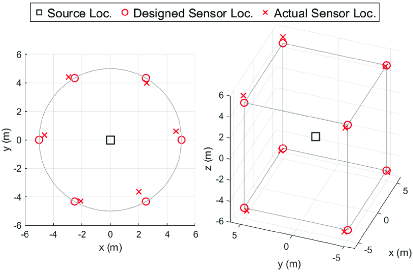
In practice, deploying sensor placement strategies, including optimal sensor placement strategies, is inevitable to encounter sensor position errors due to installation deviations or changes in sensor location caused by long-term use, etc. Fig. 1 presents 2D and 3D examples of sensor placement following a specified strategy (gray trajectory) with sensor location errors. ‘Designed Sensor Loc.’ can also be understood as the sensor locations we know, which are also regarded as the sensor location measurements. However, most works were related to optimal sensor placement without sensor location noises (OSP-WSLN), and only a few focused on optimal sensor placement with sensor location noises (OSP-SLN). [16] studied the influence of sensor location errors on the trace of CRB for TDOA-based localization. However, they only proved that the trace of CRB under sensor location errors is always larger than that of CRB without the errors and did not derive a solution to minimize the trace of CRB under sensor location errors, i.e., OSP-SLN. Very recently, in cooperative multi-robot localization, [17] studied optimal anchor (robot) placements under mobile anchor location uncertainty. They utilized range-based measurements which are different from ours. There are three main contributions to this paper:
-
•
To our best knowledge, it is the first time exploring OSP-SLN for TDOA-based localization. Minimizing the trace of CRB is used to find out the OSP-SLN strategy.
- •
-
•
We conducted simulations to show the correctness of the equality, the equivalence between OSP-WSLN and OSP-SLN, no large sensor location noises taking the ignorable influence on the performance of OSP-SLN quantified by the trace of CRB, and the contribution of OSP-SLN to improving source localization accuracy. We open-source our code to benefit the community.
II Formulation
Denote the -th sensor location as () and is the location of the sound source (). Denote measurement and measurement function for time difference of arrival (TDOA) between the -th sensor and the -th sensor are and respectively and their relationship is
| (1) |
where is the propagation velocity of source, and is Gaussian noise in . Denote TDOA measurements as () and the corresponding vector of measurement function also arrange its elements in this order. Denote measurement and measurement function of the -th sensor location are and respectively and their relationship is
| (2) |
where that is Gaussian noise. Denote sensor location measurement as and the corresponding vector of measurement function also arrange its elements in this order.
Denote as the parameter vector that needs to be estimated and is the measurement vector. When sensor locations are precisely known, , , and when sensor locations have errors, , . The maximum likelihood function is formulated as
| (3) |
where is the covariance matrix with diagonal form and is a constant. The Fisher information matrix is
| (4) |
where is the true value of . The Jacobian matrix and the CRB matrix are and respectively. Denote the CRB matrix and the Jacobian matrix with/without sensor location errors as / and / respectively. Denote and as
| (5) |
respectively where .
III Equivalence between OSP-SLN and OSP-WSLN
In this section, we first derive the concise equality describing the linear relationship between the trace of CRB for OSP-SLN and the trace of CRB for OSP-WSLN. Then, the equivalence between OSP-SLN and OSP-WSLN can be easily proven based on the equality Eq. (18).
Denote as the sub-matrix of , which represents the CRB matrix for sound location parameters. By the block matrix inversion formula and simplification, we have
| (7) | ||||
Here, . The trace of i.e., and the trace of i.e., represent the lower bound for the mean square error (MSE) of the source location with and without sensor location noises respectively. To further analyze, we expand Eq. (7) by doing the singular value decomposition (SVD) of :
| (8) |
where and unitary matrix . Then we have
| (9) |
where and . Based on Eq. (9), we simplify the trace of :
| (10) | ||||
Furthermore, a gap function between and is
| (11) | ||||
Unless otherwise specified, is used to stand for . Next, we do the SVD on :
| (12) |
where and unitary matrix . Based on Eq. (12), is simplified as
| (13) | ||||
where . By Lemma 1 demonstrated at the end of this section, . is further simplified as
| (14) | ||||
where
| (15) |
Assume and according to Lemma 2, the SVD is performed: where . Note that Lemma 2 is proven at the end of this section. Both and are unitary matrix. Note that and replace with , we get
| (16) | ||||
Therefore,
| (17) | ||||
which means
| (18) |
Therefore, without loss of generality, assume , it is easy to prove the equivalence: , which indicates that OSP-WSLN is equivalent to OSP-SLN.
Lemma 1: When is decomposed by the thin SVD i.e., Eq. (12), and .
Proof: is formulated as
| (19) |
where is a unit row vector. Denote symmetric and is full rank. The formulation of is ignored due to the limited space. An important property of is: , which can be demonstrated by calculation. Therefore, assume and are any eigenvalue and the corresponding eigenvector of respectively, . Because any eigenvector of of full rank is non-zero, . Therefore, non-zero singular values of equal to , which means .
Lemma 2: When we do the SVD on (): , .
Proof: we formulate as
| (20) |
Note that is full column rank and each column vector in is the linear combination of column vectors in . The latter can be formulated as . Using both Eq. (8) and Eq. (12), .
Because and , . Then, .
IV Simulations
We need to verify four parts: demonstrating the equality Eq. (18), the equivalence between OSP-SLN and OSP-WSLN, the tiny impact of not large sensor location errors on the performance of OSP-SLN, and the superiority of OSP-SLN in source localization. Indoor sound source localization is used as an example.
IV-A Correctness of the Equality
To fully verify the correctness of the derived equality, we randomly generate all parameters except for the sound velocity within a certain range: . The source is set at the origin and the sensor positions are randomly generated in a square space with a side length of . 100,000 Monte-Carlo simulations are performed. In each Monte-Carlo run, we record , , , and and calculate . After 100,000 Monte-Carlo simulations, the mean of equals after removing outliers in boxplot [18]. The averaged error, i.e., is inevitably caused by floating-point calculations, which indicates the concise equality Eq. (18) holds when ignoring numerical errors.
IV-B Verification of the Equivalence and Minute Impact
IV-B1 Set up
In this section, two conclusions are to be verified: the equivalence between OSP-SLN and OSP-WSLN, and the tiny impact of limited sensor location errors on the performance of deploying the OSP-SLN strategy. Under assumptions of the full set of TDOA and near-field, the OSP-WSLN in 2D space is a uniform angular array (UAA) and the OSP-WSLN in 3D space is a platonic solid [8]. UAA is set as
| (21) | ||||
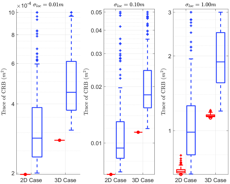
where we set , , , , . For platonic solids in 3D space, we select the cube whose and edge length equals . The source is placed at the origin. We set and . is called as when true values of sensor location precisely follow the optimal configuration. is called as when equals optimal locations adding errors. is called as when are generated randomly over a square space with a side length of . In each , 200 Monte-Carlo simulations are performed and in each simulation, , and are computed.
IV-B2 Results
The simulation results are shown in Fig. 2 and note that when in both 2D and 3D scenarios, is larger than zero and extremely small. There are two observations from Fig. 2 and the note, and these observations are consistent in both 2D and 3D cases. Firstly, is the smallest over all cases, which means OSP-SLN is equivalent to OSP-WSLN. The second one is when sensor location noises are not large (), every is close enough to and is less than all of , which supports the second conclusion in this section.
IV-C Improvement for Source Localization by OSP-SLN
IV-C1 Set up
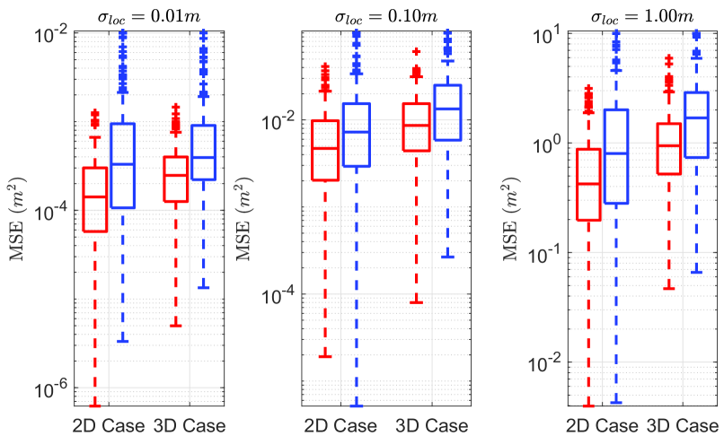
The superiority of OSP-SLN in sound source localization is verified in this section. The OSP-SLN in 2D space and the OSP-SLN in 3D space are a uniform angular array (UAA) and a platonic solid respectively, which has been demonstrated by the equivalence between OSP-SLN and OSP-WSLN. The configuration setting of UAA and platonic solid are the same as that in Section IV.B. We set and . In each , we perform 200 Monte-Carlo simulations. Each simulation generates measurements, selects initial values randomly, and localizes the sound source. To be specific, the MSE of the source location following the OSP-SLN strategy (MSE-OSP-SLN) and the MSE of the source location by placing sensors randomly (MSE-RAN) are computed. The formulation of optimization for sound source localization with sensor location errors is
| (22) |
which is solved by the Gauss-Newton (GN) method.
IV-C2 Results
The simulation results are shown in Fig. 3. We can observe that the performance of MSE-OSP-SLN is better than that of MSE-RAN in both 2D/3D space under any level of sensor location noise, which means source localization accuracy is improved by the OSP-SLN strategy significantly.
V Conclusions and Future Works
In this paper, we study the optimal sensor placement strategy for TDOA-based source localization under sensor location noises, called OSP-SLN. Under the assumptions of the full set of TDOA and near-field, OSP-SLN is shown to be equivalent to OSP-WSLN from a concise equity Eq. (18) that describes the linear relationship between the trace of CRB without sensor location errors and the trace of CRB with the errors. The other problem is how sensor location errors influence the performance of OSP-SLN policy and the answer is obtained in simulation. Extensive simulations validate both equality and equivalence and demonstrate that no large sensor location errors bring an ignorable impact on the performance quantified by the trace of CRB. Further, simulations show that deploying the OSP-SLN policy improves source localization accuracy remarkably.
In the future, we will study theoretically the impact of sensor position errors on the trace of CRB for the OSP-SLN by modeling as random variables. Also, OSP-SLN strategies will be explored based on other optimization criteria and other measurements.
References
- [1] J. Tiemann and C. Wietfeld, “Scalable and precise multi-uav indoor navigation using tdoa-based uwb localization,” in 2017 International Conference on Indoor Positioning and Indoor Navigation (IPIN), 2017, pp. 1–7.
- [2] F. Gustafsson and F. Gunnarsson, “Mobile positioning using wireless networks: possibilities and fundamental limitations based on available wireless network measurements,” IEEE Signal Processing Magazine, vol. 22, no. 4, pp. 41–53, 2005.
- [3] R. Zekavat and R. M. Buehrer, “Handbook of position location: theory, practice, and advances,” 2019.
- [4] R. O. Schmidt, “A new approach to geometry of range difference location,” IEEE Transactions on Aerospace and Electronic Systems, vol. AES-8, no. 6, pp. 821–835, 1972.
- [5] Y. Chan and K. Ho, “A simple and efficient estimator for hyperbolic location,” IEEE Transactions on Signal Processing, vol. 42, no. 8, pp. 1905–1915, 1994.
- [6] K. Ho and Y. Chan, “Solution and performance analysis of geolocation by tdoa,” IEEE Transactions on Aerospace and Electronic Systems, vol. 29, no. 4, pp. 1311–1322, 1993.
- [7] K. C. Ho and L. M. Vicente, “Sensor allocation for source localization with decoupled range and bearing estimation,” IEEE Transactions on Signal Processing, vol. 56, no. 12, pp. 5773–5789, 2008.
- [8] B. Yang and J. Scheuing, “Cramer-rao bound and optimum sensor array for source localization from time differences of arrival,” in Proceedings. (ICASSP ’05). IEEE International Conference on Acoustics, Speech, and Signal Processing, 2005., vol. 4, 2005, pp. iv/961–iv/964 Vol. 4.
- [9] ——, “A theoretical analysis of 2d sensor arrays for tdoa based localization,” in 2006 IEEE International Conference on Acoustics Speech and Signal Processing Proceedings, vol. 4, 2006, pp. IV–IV.
- [10] B. Yang, “Different sensor placement strategies for tdoa based localization,” in 2007 IEEE International Conference on Acoustics, Speech and Signal Processing - ICASSP ’07, vol. 2, 2007, pp. II–1093–II–1096.
- [11] A. N. Bishop, B. Fidan, B. D. Anderson, P. N. Pathirana, and K. Dogancay, “Optimality analysis of sensor-target geometries in passive localization: Part 2 - time-of-arrival based localization,” in 2007 3rd International Conference on Intelligent Sensors, Sensor Networks and Information, 2007, pp. 13–18.
- [12] J. T. Isaacs, D. J. Klein, and J. P. Hespanha, “Optimal sensor placement for time difference of arrival localization,” in Proceedings of the 48h IEEE Conference on Decision and Control (CDC) held jointly with 2009 28th Chinese Control Conference, 2009, pp. 7878–7884.
- [13] K. Panwar, G. Fatima, and P. Babu, “Optimal sensor placement for hybrid source localization using fused toa–rss–aoa measurements,” IEEE Transactions on Aerospace and Electronic Systems, vol. 59, no. 2, pp. 1643–1657, 2023.
- [14] K. Tang, S. Xu, Y. Yang, H. Kong, and Y. Ma, “Optimal sensor placement using combinations of hybrid measurements for source localization,” in 2024 IEEE Radar Conference (RadarConf24), 2024, pp. 1–6.
- [15] N. Sahu, L. Wu, P. Babu, B. S. M. R., and B. Ottersten, “Optimal sensor placement for source localization: A unified admm approach,” IEEE Transactions on Vehicular Technology, vol. 71, no. 4, pp. 4359–4372, 2022.
- [16] Y. Yang, J. Zheng, H. Liu, K. Ho, Y. Chen, and Z. Yang, “Optimal sensor placement for source tracking under synchronization offsets and sensor location errors with distance-dependent noises,” Signal Processing, vol. 193, p. 108399, 2022. [Online]. Available: https://www.sciencedirect.com/science/article/pii/S0165168421004369
- [17] M. Theunissen, I. Fantoni, E. Malis, and P. Martinet, “Robustness study of optimal geometries for cooperative multi-robot localization,” in IEEE/RSJ International Conference on Intelligent Robots and Systems., 2024.
- [18] F. M. Dekking, C. Kraaikamp, H. P. Lopuhaä, and L. E. Meester, “A modern introduction to probability and statistics,” Springer Texts in Statistics, 2005.