Generator Matching: Generative modeling with arbitrary Markov processes

Abstract

We introduce generator matching, a modality-agnostic framework for generative modeling using arbitrary Markov processes. Generators characterize the infinitesimal evolution of a Markov process, which we leverage for generative modeling in a similar vein to flow matching: we construct conditional generators which generate single data points, then learn to approximate the marginal generator which generates the full data distribution. We show that generator matching unifies various generative modeling methods, including diffusion models, flow matching and discrete diffusion models. Furthermore, it provides the foundation to expand the design space to new and unexplored Markov processes such as jump processes. Finally, generator matching enables the construction of superpositions of Markov generative processes and enables the construction of multimodal models in a rigorous manner. We empirically validate our method on protein and image structure generation, showing that superposition with a jump process improves image generation.

1 Introduction

Early deep generative models—like VAEs (Kingma, 2013) and GANs (Goodfellow et al., 2014) generated samples in a single forward pass. With denoising diffusion models (DDMs) (Song et al., 2020; Ho et al., 2020), a paradigm shift happened were step-wise updates are used to transform noise into data. Similarly, scalable training of continuous normalizing flows (CNFs; Chen et al. 2018) via flow matching (Lipman et al., 2022; Liu et al., 2022; Albergo et al., 2023) allowed for high-quality and fast generative modeling by simulating an ODE. Since then, similar constructions based on diffusion and flows have also been applied to other modalities such as discrete data (Campbell et al., 2022; Gat et al., 2024) or data on manifolds (De Bortoli et al., 2022; Huang et al., 2022; Chen & Lipman, 2024) leading to a variety of models for different data types.

The single common property of the aforementioned generative models is their iterative step-wise nature: starting with a sample $X_{0}\sim p_{\text{simple}}$ from an easy-to-sample distribution $p_{\text{simple}}$, they iteratively construct samples $X_{t+h}$ of the next time step depending only on the current state $X_{t}$. Mathematically speaking, this means that they are all Markov processes. In this work, we develop a generative modeling framework that solely relies on that Markov property. At the core of our framework is the concept of a generator that describes the infinitesimal change of the distribution of a Markov process. We show that one can easily learn a generator through a family of scalable training objectives—a framework we coin generator matching (GM).

Generator matching unifies many existing generative modeling techniques across modalities such as denoising diffusion models (Song et al., 2020), flow matching (Lipman et al., 2022), stochastic interpolants (Albergo et al., 2023), discrete diffusion models (Campbell et al., 2022; Gat et al., 2024; Lou et al., 2024a), among many others (see sec. 8). Most importantly, GM gives rise to new, unexplored models, and allows us to combine models across different classes of Markov processes. We make the following contributions:

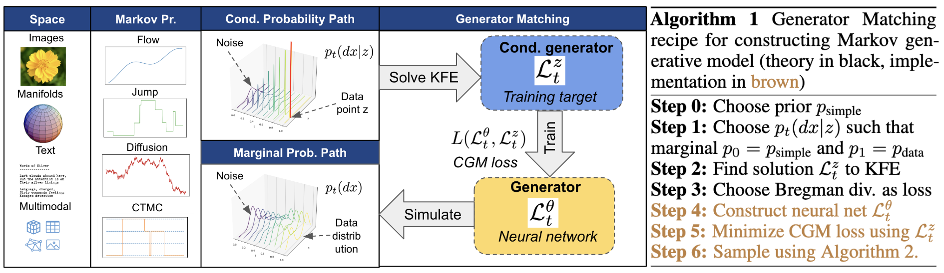
Figure 1: Overview of the generator matching (GM) framework to construct generative models. GM works on any state space (including multi-modal) and Markov processes. Flower image source: vecteezy.com

1. Generator matching: We present generator matching, a framework for generative modeling with Markov processes on arbitrary state spaces. This framework unifies a diversity of prior generative modeling methods into a common framework that is modality-agnostic.

2. Novel models: We universally characterize the space of Markovian generative models on discrete and Euclidean spaces identifying jump models as an unexplored model class for $\mathbb{R}^{d}$.

3. Model combinations: We show how generator matching allows to combine models in 2 ways: (1) We introduce Markov superpositions for generative models on the same state space; and (2) We build multimodal generative models by combining unimodal generators.

4. Experiments: On image and protein structure generation experiments, we show that jump models and Markov superpositions allow us to achieve competitive results.

2 Generative modeling via Probability Paths

Let $S$ be a state space. Important examples are $S=\mathbb{R}^{d}$ (e.g., images, vectors), $S$ discrete (e.g., language), $S$ a Riemannian manifold (e.g., geometric data) or their products for multimodal data generation. In generative modeling, we are given samples $x_{1},\dots,x_{N}\sim p_{\text{data}}$ from a distribution $p_{\text{data}}$ on $S$ and our goal is to generate novel samples $z\sim p_{\text{data}}$. GM works for arbitrary distributions, in particular those that do not have densities (e.g., with discrete support). If for a distribution $p$ a density exists, we write $p(x)$ for its density and consider $p$ as a function $p:S\to\mathbb{R}_{\geq 0}$. For general probability measures $p$, we use the notation $p(dx)$ where "$dx$" is a symbolic expression denoting integration with respect to $p$ in a variable $x$. For a reader unfamiliar with the notation, one can simply assume the density exists and simply read $p(dx)=p(x)dx$.

A fundamental paradigm of recent state-of-the-art generative models is that they prespecify a transformation of a simple distribution $p_{\text{simple}}$ (e.g. a Gaussian) into $p_{\text{data}}$ via probability paths. Specifically, a conditional probability path is a set of time-varying probability distributions $(p_{t}(dx|z))_{0\leq t\leq 1}$ depending on a data point $z\in S$. The data distribution $p_{\text{data}}$ induces a corresponding marginal probability path

$$p_{t}(dx)=\mathbb{E}_{z\sim p_{\text{data}}}[p_{t}(dx|z)]$$

The main feature of the conditional probability path $p_{t}(dx|z)$ is that it is easy to sample from. Given a dataset of samples from $p_{\text{data}}$, one can then also efficiently draw samples from the marginal $p_{t}(dx)$: first sample a data point $z\sim p_{\text{data}}$ and then sample $x\sim p_{t}(dx|z)$. As we will see, this makes training scalable.

The key design requirement for the conditional probability path is that its associated marginal probability path interpolates between $p_{\text{simple}}$ and $p_{\text{data}}$, leading to the first design principle of GM:

Principle 1: Given a data distribution $p_{\text{data}}$, choose a prior $p_{\text{simple}}$ and a conditional probability path such that its marginal probability path $(p_{t})_{0\leq t\leq 1}$ fulfills $p_{\text{simple}}=p_{0}$ and $p_{\text{data}}=p_{1}$.

Two common constructions are mixtures (for arbitrary $S$) and geometric averages (for $S=\mathbb{R}^{d}$):

$$p_{t}(dx|z) =(1-\kappa_{t})\cdot p_{\text{simple}}(dx)+\kappa_{t}\cdot\delta_{z}(dx)\ \ \Leftrightarrow\ \ x_{t}\sim\begin{cases}z&\text{with prob }\kappa_{t}\\ x_{0}&\text{with prob }(1-\kappa_{t})\end{cases}\ \ \blacktriangleright\text{mixture}$$

$$p_{t}(dx|z) =\mathbb{E}_{x_{0}}\left[\delta_{\sigma_{t}x_{0}+\alpha_{t}z}\right]\quad\qquad\ \ \qquad\qquad\ \ \ \Leftrightarrow\ \ x_{t}=\sigma_{t}x_{0}+\alpha_{t}z\quad\quad\ \blacktriangleright\text{geometric average}$$

where $x_{t}\sim p_{t}(\cdot|z),x_{0}\sim p_{\text{simple}},z\sim p_{\text{data}}$, and $\alpha_{t},\sigma_{t},\kappa_{t}\in\mathbb{R}_{\geq 0}$ are differentiable functions satisfying $\kappa_{0}=\alpha_{0}=\sigma_{1}=0$ and $\kappa_{1}=\alpha_{1}=\sigma_{0}=1$ and $0\leq\kappa_{t}\leq 1$.

Remark. Our time parameterization follows the standard from the flow literature where $t=1$ corresponds to data and $t=0$ corresponds to noise. In the diffusion literature, time is inverted ($t=0$ corresponds to data) and a probability path is modelled as a forward diffusion process. Further, GM also works if one conditions a probability path on start and end point (Tong et al., 2023; Pooladian et al., 2023).

3 Markov Processes

We briefly time-continuous Markov processes, a fundamental concept in this work (Ethier & Kurtz, 2009). For $t\in[0,1]$, let $X_{t}\in S$ be a random variable. We call $(X_{t})_{0\leq t\leq 1}$ a Markov process if it fulfills the following condition for all $0\leq t_{1}<t_{2}<\dots<t_{n}<t_{n+1}\leq 1$ and $A\subseteq S$ (measurable):

$$\mathbb{P}[X_{t_{n+1}}\in A|X_{t_{1}},X_{t_{2}},\dots,X_{t_{n}}]=\mathbb{P}[X_{t_{n+1}}\in A|X_{t_{n}}] \blacktriangleright\text{Markov assumption}$$

Informally, the above condition says that the process has no memory. If we know the present, knowing the past will not influence our prediction of the future. In table 1, we give an overview over important classes of Markov processes. Each Markov process has a transition kernel $(k_{t+h|t})_{0\leq t<t+h\leq 1}$ that assigns every $x\in S$ a probability distribution $k_{t+h|t}(\cdot|x)$ such that $\mathbb{P}[X_{t+h}\in A|X_{t}=x]=k_{t+h|t}(A|x)$. Due to the Markov assumption, a Markov process is fully specified by a transition kernel and its initial distribution $p_{0}$. Conversely, any initial distribution and transition kernel define a Markov process.

In the context of GM, we use a Markov process as follows: Given a marginal path $(p_{t}(dx))_{0\leq t\leq 1}$ (see sec. 2), we want to train a model that allows to simulate a Markov process such that $X_{0}\sim p_{\text{simple}}\Rightarrow X_{t}\sim p_{t}\quad\text{for all }0\leq t\leq 1$. That is, if starting with the right initial distribution $X_{0}\sim p_{0}$, the marginals of $X_{t}$ will be $p_{t}$. Once we have found such a Markov process, we can simply generate samples from $p_{1}=p_{\text{data}}$ by sampling $X_{0}\sim p_{0}$ and simulating $X_{t+h}\sim k_{t+h|t}(\cdot|X_{t})$ step-wise up to time $t=1$. The challenge with such an approach is that an arbitrary general kernel $k_{t+h|t}$ is hard to parameterize in a neural network. One of the key insights in the development diffusion models was that for small $h>0$, the kernel $k_{t+h|t}$ can be closely approximated by a simple parametric distribution like Gaussian (Sohl-Dickstein et al., 2015; Ho et al., 2020). One can extend this idea to Markov processes leading to the concept of the generator.

Name Flow Diffusion Jump process Continous-time Markov chain Space $S$ $S=\mathbb{R}^{d}$ $S=\mathbb{R}^{d}$ $S$ arbitrary $|S|<\infty$ Parameters $u_{t}(x)\in\mathbb{R}^{d}$ $\sigma_{t}^{2}(x)\in S_{d}^{++}$ Jump measure $Q_{t}(dy;x)\geq 0$ $Q_{t}\in\mathbb{R}^{S\times S}$, $1^{T}Q_{t}=0$ $Q_{t}(x^{\prime};x)\geq 0$ ($x^{\prime}\neq x$) Sampling $X_{t+h}=X_{t}+hu_{t}(X_{t})$ $X_{t+h}=X_{t}+\sqrt{h\sigma_{t}^{2}(X_{t})}\epsilon_{t}$ $\epsilon_{t}\sim\mathcal{N}(0,I)$ $X_{t+h}=X_{t}$ with prob. $1-h\int Q_{t}(dy;x)$ $X_{t+h}\sim\frac{Q_{t}(dy;x)}{\int Q_{t}(dy;x)}$ with prob. $h\int Q_{t}(dy;x)$ $X_{t+h}\sim(I+hQ_{t})(\cdot;X_{t})$ Generator $\mathcal{L}_{t}$ $\nabla f^{T}u_{t}$ $\frac{1}{2}\nabla^{2}f\cdot\sigma_{t}^{2}$ $\int f(y)-f(x)Q_{t}(dy;x)$ $f^{T}Q_{t}^{T}$ KFE (Adjoint) Continuity Equation: $\partial_{t}p_{t}=-\nabla\cdot[u_{t}p_{t}]$ Fokker-Planck Equation: $\partial_{t}p_{t}=\frac{1}{2}\nabla^{2}\cdot[p_{t}\sigma^{2}_{t}]$ Jump Continuity Equation: $\partial_{t}p_{t}(x)=$ $\int Q_{t}(x;x^{\prime})p_{t}(x^{\prime})-Q_{t}(x^{\prime};x)p_{t}(x)dx^{\prime}$ Mass preservation: $\partial_{t}p_{t}=Q_{t}p_{t}$ Marginal $\mathbb{E}_{z\sim p_{1|t}(\cdot|x)}[u_{t}(x|z)]$ $\mathbb{E}_{z\sim p_{1|t}(\cdot|x)}[\sigma_{t}^{2}(x|z)]$ $\mathbb{E}_{z\sim p_{1|t}(\cdot|x)}[Q_{t}(dx^{\prime};x|z)]$ $\mathbb{E}_{z\sim p_{1|t}(\cdot|x)}[Q_{t}(x^{\prime};x|z)]$ CGM Loss (Example) $\|u_{t}(x|z)-u_{t}^{\theta}(x)\|^{2}$ $\|\sigma_{t}^{2}(x|z)-[\sigma_{t}^{\theta}]^{2}(x)\|_{2}^{2}$ $(\int Q_{t}^{\theta}(x^{\prime};x)dx^{\prime}$ $-Q_{t}(x^{\prime};x|z)\log Q_{t}^{\theta}(x^{\prime};x)dx^{\prime})$ $(\sum\limits_{x^{\prime}\neq x}Q_{t}^{\theta}(x^{\prime};x)$ $-Q_{t}(x^{\prime};x|z)\log Q_{t}^{\theta}(x^{\prime};x))$

Table 1: Overview of various classes of Markov processes, their generators and how they are learnt with GM. Derivations can be found in sec. A.4. For diffusion, we assume zero drift as this is captured by the flow column. KFE is listed in its adjoint version, i.e. assumes density $p_{t}(x)$ and jump kernel $Q_{t}(y;x)$ exists.

4 Generators

Let us consider the transition kernel $k_{t+h|t}$ for small $h>0$. Specifically, we consider an informal 1st-order Taylor approximation in $t$ with an error term $o(h)$:

$$``k_{t+h|t}=k_{t|t}+h\mathcal{L}_{t}+o(h)",\quad\mathcal{L}_{t}:=\frac{d}{dh}\Big{|}_{h=0}k_{t+h|t},\quad k_{t|t}(\cdot|x)=\delta_{x}$$ (1)

We call the 1st-order derivative $\mathcal{L}_{t}$ the generator of $k_{t+h|t}$ (Ethier & Kurtz, 2009; Rüschendorf et al., 2016). Similar to derivatives, generators are first-order linear approximations and, as we will see, easier to parameterize than $k_{t+h|t}$. As we will see, diffusion, flow, and other generative models can all be seen as algorithms to learn the generator of a Markov process (see table 1). However, as a probability measure is not a standard function, equation 1 is not well-defined yet. We will make it rigorous using test functions.

Test functions. Test functions are a way to “probe” a probability distribution. They serve as a theoretical tool to handle distributions as if they were real-valued functions. Specifically, we use a family $\mathcal{T}$ of bounded, integrable functions $f:S\to\mathbb{R}$ that characterize probability distributions fully, i.e., two probability distributions $\mu_{1},\mu_{2}$ are equal if and only if $\mathbb{E}_{x\sim\mu_{1}}[f(x)]=\mathbb{E}_{x\sim\mu_{2}}[f(x)]$ for all $f\in\mathcal{T}$. Generally speaking, one chooses $\mathcal{T}$ to be as “nice” (or regular) as possible. For example, if $S=\mathbb{R}^{d}$, the space $\mathcal{T}=C_{c}^{\infty}$ of infinitely differentiable functions with compact support fulfills that property. We define the action of the marginal $p_{t}$ and transition kernels $k_{t+h|t}$ for all $f\in\mathcal{T}$ via

$$p_{t}\odot f =\int f(y)p_{t}(dy)=\mathbb{E}\left[f(X_{t})\right] \blacktriangleright\text{marginal action}$$ (2)

$$\left[k_{t+h|t}\odot f\right](x) =\int f(y)k_{t+h|t}(dy|x)=\mathbb{E}\left[f(X_{t+h})|X_{t}=x\right] \blacktriangleright\text{transition action}$$ (3)

where the marginal action maps each test function $f$ to a scalar $p_{t}\odot f\in\mathbb{R}$, while the transition action maps a real-valued function $x\mapsto f(x)$ to a another real-valued function $x\mapsto[k_{t+h|t}\odot f](x)$. The tower property implies that $p_{t}\odot[k_{t+h|t}\odot f]=p_{t+h}\odot f$.

Generator definition.

Let us revisit equation 1 and define the derivative of $k_{t+h|t}$. With the test function perspective in mind, we can take derivatives of $\left[k_{t+h|t}\odot f\right](x)$ per $x\in S$ and define

$$\frac{d}{dh}\Big{|}_{h=0}\left[k_{t+h|t}\odot f\right](x) =\lim_{h\rightarrow 0}\frac{\left[k_{t+h|t}\odot f\right](x)-f(x)}{h}\stackrel{{\scriptstyle\text{def}}}{{=}}[{\mathcal{L}}_{t}f](x).$$ (4)

We call this action the generator ${\mathcal{L}}_{t}$ (and define it for all $f$ for which the limit exists uniformly in $x$ and $t$, see sec. A.1 ). In table 1, there are several examples of generators listed with derivations in sec. A.4. With this definition, the Taylor series in equation 1 has the, now well-defined, form as $k_{t+h|t}\odot f=f+h{\mathcal{L}}_{t}f+o(h)$.

Under mild regularity assumptions, there is a unique correspondence between the generator and the Markov process (Ethier & Kurtz, 2009; Pazy, 2012). This allows us to parameterize a Markov process:

Principle 2: Parameterize a Markov process via a parameterized generator $\mathcal{L}_{t}^{\theta}$.

Of course, it is hard to parameterize a linear operator $\mathcal{L}_{t}$ on function spaces directly via a neural network. A simple solution is to restrict ourselves to certain subclasses of Markov processes and parameterize it linearly with a neural network (see sec. A.5 for details and examples). For example, flow matching restricts itself to generators of the form $\mathcal{L}_{t}f=\nabla f(x)^{T}u_{t}^{\theta}(x)$ which correspond to flows. However, as we will show now, we can in fact fully characterize generators on specific spaces.

Theorem 1 (Universal characterization of generators).

Under regularity assumptions (see sec. A.2), the generators of a Markov processes $X_{t}$ ($0\leq t\leq 1$) take the form:

1. Discrete $|S|<\infty$: The generator is given by a rate transition matrix $Q_{t}$ and the Markov process corresponds to a continuous-time Markov chain (CTMC).

2. Euclidean space $S=\mathbb{R}^{d}$: The generator has a representation as a sum of components described in table 1, i.e.,

   $$\mathcal{L}_{t}f(x)=\underbrace{\vphantom{\frac{1}{2}}\nabla f(x)^{T}u_{t}(x)}_{\text{flow}}+\underbrace{\frac{1}{2}\nabla^{2}f(x)\cdot\sigma^{2}_{t}(x)}_{\text{diffusion}}+\underbrace{\int\left[f(y)-f(x)\right]Q_{t}(dy;x)}_{\text{jump}}$$ (5)

   where $u:[0,1]\times\mathbb{R}^{d}\rightarrow\mathbb{R}^{d}$ is a velocity field, $\sigma:[0,1]\times\mathbb{R}^{d}\rightarrow S^{++}_{d}$ the diffusion coefficient ($S^{++}_{d}$=positive semi-definite matrices), and $Q_{t}(A|x)$ is a finite measure called jump measure. $\nabla^{2}f(x)$ describes the Hessian of $f$ and $\nabla^{2}f(x)\cdot\sigma^{2}_{t}(x)$ describes the Frobenius inner product.

The proof adapts a known result in the mathematical literature and can be found in sec. C.1. This result allows us to not only characterize a wide class of Markov process models but to characterize the design space exhaustively for $S=\mathbb{R}^{d}$ or $S$ discrete. In Euclidean space, people have considered learning the flow parts of the generator and for diffusion models, using a fixed $\sigma_{t}$ for a diffusion. Learning $\sigma_{t}$ or jump models on non-discrete spaces have not (or rarely) been considered. A general recipe to sample from a Markov process with a universal generator is presented in alg. 2. For $S=\mathbb{R}^{d}$, we can therefore simplify Principle 2:

Principle 2 ($S=\mathbb{R}^{d})$: Parameterize a Markov process (e.g., using a neural network) via a generator $\mathcal{L}_{t}$ that is composed of (a subset of) velocity $u_{t}$, diffusion coefficient $\sigma_{t}^{2}$, and jump measure $Q_{t}$.

5 Kolmogorov Forward Equation and Marginal Generator

Beyond parameterizing a Markov process, the generator has a further use-case in the generator matching framework: checking if a Markov process generates a desired probability path $p_{t}$. We discuss the latter now using the Kolmogorov Forward Equation (KFE). Specifically, the evolution of the marginal probabilities $p_{t}$ of a Markov process $X_{t}$ are governed by the generator ${\mathcal{L}}_{t}$, as can be seen by computing:

$$\partial_{t}[p_{t}\odot f]= \frac{d}{dh}\Big{|}_{h=0}[p_{t+h}\odot f]=\frac{d}{dh}\Big{|}_{h=0}p_{t}\odot\left[k_{t+h|t}\odot f\right]=p_{t}\odot\left[\frac{d}{dh}\Big{|}_{h=0}k_{t+h|t}\odot f\right]\overset{(\ref{e:generator})}{=}p_{t}\odot{\mathcal{L}}_{t}f,$$

where we used that the $p_{t}\odot$ operation is linear to swap the derivative, and the fact that $p_{t}\odot[k_{t+h|t}\odot f]=p_{t+h}\odot f$. This shows that given a generator ${\mathcal{L}}_{t}$ of a Markov process $X_{t}$ we can recover its marginal probabilities via their infinitesimal change,

$$\partial_{t}[p_{t}\odot f]=p_{t}\odot[{\mathcal{L}}_{t}f]\qquad\blacktriangleright\text{Kolmogorov Forward Equation (KFE)}$$ (6)

Conversely, if a generator ${\mathcal{L}}_{t}$ of a Markov process $X_{t}$ satisfies the above equation, then $X_{t}$ generates the probability path $(p_{t})_{0\leq t\leq 1}$, i.e. initializing $X_{0}\sim p_{0}$ will imply that $X_{t}\sim p_{t}$ for all $0\leq t\leq 1$ (see item 5) (Rogers & Williams, 2000). Therefore, a key component of the Generator Matching framework will be:

Principle 3*: Given a marginal probability path $(p_{t})_{0\leq t\leq 1}$, find a generator satisfying the KFE.

Adjoint KFE. The above version of the KFE determines the evolution of expectations of test functions $f$. Whenever a probability density $p_{t}(x)$ exists, one can use the adjoint KFE (see table 1 for examples and sec. A.3 for details). In this form, the KFE generalizes many equations used to develop generative models such as Fokker-Planck or the continuity equation (Song et al., 2020; Lipman et al., 2022) (see table 1).

As we will show in the next proposition, to find a Markov process that generates the marginal probability path, we only need to find one that generates the conditional path.

Proposition 1.

For every data point $z\in S$, let $X_{t}^{z}$ be a Markov process with generator $\mathcal{L}_{t}^{z}$ that we call conditional generator. Assume that $X_{t}^{z}$ generates the conditional probability path $(p_{t}(\cdot|z))_{0\leq t\leq 1}$. Then the marginal probability path $(p_{t})_{0\leq t\leq 1}$ is generated by a Markov process $X_{t}$ with generator

$$\mathcal{L}_{t}f(x)= \mathbb{E}_{z\sim p_{1|t}(\cdot|x)}[\mathcal{L}_{t}^{z}f(x)]$$ (7)

where $p_{1|t}(dz|x)$ is the posterior distribution (i.e. the conditional distribution over data $z$ given an observation $x$). For $S=\mathbb{R}^{d}$ and the representation in eq. 5, we get a marginal representation of $\mathcal{L}_{t}f(x)$ given by:

$$\nabla f(x)^{T}\mathbb{E}_{z\sim p_{1|t}(\cdot|x)}[u_{t}(x|z)]+\frac{\nabla^{2}f(x)}{2}\cdot\mathbb{E}_{z\sim p_{1|t}(\cdot|x)}[\sigma_{t}^{2}(x|z)]+\int\left[f(y)-f(x)\right]\mathbb{E}_{z\sim p_{1|t}(\cdot|x)}[Q_{t}(dy;x|z)]$$

More generally, an identity as in eq. 7 holds for any linear parameterization of the generator (see sec. C.3).

The proof relies on the linearity of the KFE (see sec. C.3). Proposition 1 immensely simplifies the construction of a Markov process that generates a desired probability path. To find the right training target, we only need to find a solution for the KFE for the conditional path. This simplifies Principle 3* to:

Principle 3: Derive a conditional generator ${\mathcal{L}}_{t}^{z}$ satisfying the KFE for the conditional path $p_{t}(\cdot|z)$.

In denoising diffusion models, the strategy to find solutions to a KFE is to construct a probability path via a forward noising process and then use a time-reversal of that process as a solution to the KFE (we illustrate this in sec. H.2). Here, we illustrate two novel solutions for the KFE for common conditional probability paths on $\mathbb{R}^{d}$ in fig. 2. We discuss them here for $d=1$ (in sec. 7.2 it is discussed how to easily extend it to $d>1$).

Example 1 - Jump solution to geometric average. Current state-of-the-art models use a geometric average probability path of the form $p_{t}(x|z)=\mathcal{N}(x;tz,(1-t)^{2})$ called CondOT path (Lipman et al., 2022). We ask the question: are there other Markov processes that follow the same probability path? As derived in sec. E.1, another solution is given by a jump model with rate kernel $Q_{t}:\mathbb{R}\times\mathbb{R}\to\mathbb{R}$:

$$Q_{t}(x^{\prime};x|z)=\frac{[k_{t}(x)]_{+}[-k_{t}(x^{\prime})]_{+}p_{t}(x^{\prime}|z)}{(1-t)^{3}\int[-k_{t}(\tilde{x})]_{+}p_{t}(\tilde{x}|z)d\tilde{x}},\quad k_{t}(x)=x^{2}-(t+1)xz-(1-t)^{2}+tz^{2}$$ (8)

where $[x]_{+}:=\max(x,0)$. In fig. 2, we illustrate how a jump model trained with this conditional rate has the same marginal probability path as common flow models but with significantly different sample paths.

Example 2 - Pure diffusion solution to mixture path. GM allows to learn the diffusion coefficient $\sigma_{t}^{2}$ of an SDE. We illustrate this for the mixture path $p_{t}(dx|z)=\kappa_{t}\delta_{z}+(1-\kappa_{t})\text{Unif}_{[a_{1},a_{2}]}$. We introduce a solution that we call “pure diffusion” (see sec. E.2). The corresponding Markov process is given by an SDE with no drift (i.e., no vector field) and diffusion coefficient given by

$$\sigma_{t}^{2}(x|z)= 2\dot{\kappa}_{t}\frac{a_{2}-a_{1}}{1-\kappa_{t}}\left(\frac{1}{2}\frac{(x_{1}-a_{1})^{2}}{a_{2}-a_{1}}+[x-z]_{+}-\frac{1}{2}\frac{(x-a_{1})^{2}}{a_{2}-a_{1}})\right)$$ (9)

We add an additional reflection term at the boundaries of the data support (see sec. E.2 for details). Note the striking feature of this model: It only specifies how much noise to add to the current state. Still, it is able to generate data (see fig. 2). This is strictly different than “denoising diffusion models” because they corrupt data (as opposed to generating) with a diffusion process and there $\sigma_{t}^{2}(x)=\sigma_{t}^{2}$ is state-independent.

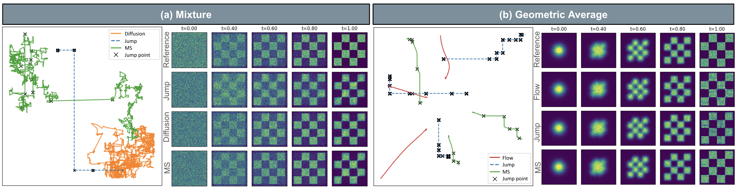
Figure 2: Illustration of Markov models trained with different KFE solutions for the same probability path. The paths for individual samples are plotted across time in one plot. 2d histograms of generated samples are plotted per time point. Although the individual sample paths look very different, the marginal probability path (histogram) are the same up to approximation error (Geometric average $\sim$ example 1, mixture $\sim$ example 2).

6 Generator Matching

We now discuss how to train a parameterized generator $\mathcal{L}_{t}^{\theta}$ to approximate the “true” marginal generator $\mathcal{L}_{t}$. In practice, $\mathcal{L}_{t}^{\theta}$ is linearly parameterized by a neural network $F_{t}^{\theta}:S\times[0,1]\to\Omega$ where $\Omega\subset V$ is convex subset of some vector space $V$ with inner product $\left\langle\cdot,\cdot\right\rangle$ (see sec. A.5 for details). Our goal is to approximate the ground truth parameterization $F_{t}:S\times[0,1]\to\Omega$ of $\mathcal{L}_{t}$. For example, $F_{t}=u_{t}$ for flows, $F_{t}=\sigma_{t}^{2}$ for diffusion, or $F_{t}=Q_{t}$ for jumps (see table 1). We train the neural network $F_{t}^{\theta}$ to approximate $F_{t}$. As a distance function on $\Omega$, we consider Bregman divergences defined via a convex function $\phi:\Omega\to\mathbb{R}$ as

$$D(a,b)=\phi(a)-[\phi(b)+\left\langle a-b,\nabla\phi(b)\right\rangle],\quad a,b\in\Omega$$ (10)

which are a general class of loss functions including many examples such as MSE or the KL-divergence (see sec. C.4.1). We use $D$ to measure how well $F_{t}^{\theta}$ approximates $F_{t}$ via the generator matching loss defined as

$$L_{\text{gm}}(\theta)\stackrel{{\scriptstyle\text{def}}}{{=}}\mathbb{E}_{t\sim\text{Unif},x\sim p_{t}}\left[D(F_{t}(x),F_{t}^{\theta}(x))\right] \blacktriangleright\text{ Generator matching}$$

Unfortunately, the above training objective is intractable as we do not know the marginal generator $\mathcal{L}_{t}$ and also no parameterization $F_{t}$ of the marginal generator. To make training tractable, let us set $F_{t}^{z}$ to be a linear parameterization of the conditional generator $\mathcal{L}_{t}^{z}$ with data point $z$ (see sec. A.5). For clarity, we reiterate that by construction, we know $F_{t}^{\theta},F_{t}^{z},p_{t}(\cdot|z),D$ as well as can draw $\text{data samples }z\sim p_{\text{data}}$ but the shape of $F_{t}$ is unknown. By proposition 1, we can assume that $F_{t}$ has the shape $F_{t}(x)=\int F^{z}_{t}(x)p_{1|t}(dz|x)$. This enables us to define the conditional generator matching loss as

$$L_{\text{cgm}}(\theta) \stackrel{{\scriptstyle\text{def}}}{{=}}\mathbb{E}_{t\sim\text{Unif},z\sim p_{\text{data}},x\sim p_{t}(\cdot|z)}\left[D(F^{z}_{t}(x),F_{t}^{\theta}(x))\right] \blacktriangleright\text{ Conditional generator matching}$$

This objective is tractable and scalable. It turns out that we can use it to minimize the desired objective.

Proposition 2.

For any Bregman divergence, the GM loss $L_{\text{gm}}$ has the same gradients as the CGM loss $L_{\text{cgm}}$, i.e. $\nabla_{\theta}L_{\text{gm}}(\theta)=\nabla_{\theta}L_{\text{cgm}}(\theta)$. Therefore, minimizing the CGM loss with Stochastic Gradient Descent will also minimize the GM loss. Further, for this property to hold, $D$ must necessarily be a Bregman divergence.

Note the significance of proposition 2: we can learn $\mathcal{L}_{t}$ without having ever access to it with a scalable objective. Further, we can universally characterize the space of loss functions. The proof can be found in sec. C.4. In table 1, we list examples of several CGM loss functions. Often it is also possible to derive losses that give upper bounds on the model log-likelihood (ELBO bounds). We illustrate this in app. D.

Principle 4: Train $\mathcal{L}_{t}^{\theta}$ by minimizing the CGM loss with a Bregman divergence.

With this, we arrived at the last principle of GM. In alg. 1, we summarize the generator matching recipe for constructing generative models.

7 Applications of generative matching theory

GM provides a unifying framework for many existing generative models (see sec. 8), as well as gives rise to new models. Beyond that, the generality of GM in itself has several use cases that we discuss in this section.

7.1 Combining models

The generator is a linear operator and the KFE $\partial_{t}[p_{t}\odot f]=p_{t}\odot[\mathcal{L}_{t}f]$ is a linear equation. These two properties enable us to combine generative models for the same state space $S$ in different ways.

Proposition 3 (Combining models).

Let $p_{t}$ be a marginal probability path, then the following generators solve the KFE for $p_{t}$ and consequently define a generative model with $p_{t}$ as marginal:

1. Markov superposition: $\alpha_{t}^{1}\mathcal{L}_{t}+\alpha^{2}_{t}\mathcal{L}_{t}^{\prime}$, where $\mathcal{L}_{t},\mathcal{L}_{t}^{\prime}$ are two generators of Markov processes solving the KFE for $p_{t}$, and $\alpha_{t}^{1},\alpha_{t}^{2}\geq 0$ satisfy $\alpha^{1}_{t}+\alpha^{2}_{t}=1$. We call this a Markov superposition.

2. Divergence-free components: $\mathcal{L}_{t}+\beta_{t}\mathcal{L}_{t}^{\text{div}}$, where $\mathcal{L}_{t}^{\text{div}}$ is a generator such that $p_{t}\odot[\mathcal{L}_{t}^{\text{div}}f]=0$ for all $f\in{\mathcal{T}}$, and $\beta_{t}\geq 0$. We call such $\mathcal{L}_{t}^{\text{div}}$ divergence-free.

3. Predictor-corrector: $\alpha^{1}_{t}\mathcal{L}_{t}+\alpha^{2}_{t}\bar{\mathcal{L}}_{t}$, where $\mathcal{L}_{t}$ is a generator solving the KFE for $p_{t}$ in forward-time and $\bar{\mathcal{L}}_{t}$ is a generator solving the KFE in backward time, and $\alpha_{t}^{1},\alpha_{t}^{2}\geq 0$ with $\alpha^{1}_{t}-\alpha^{2}_{t}=1$.

A proof can be found in sec. C.5. Markov superpositions can be used to combine generative models of different classes, e.g., one could combine a flow and a jump model. These can be 2 networks trained separately or we can train two models in one network simultaneously. We illustrate Markov superpositions in fig. 2. To find divergence-free components, one can use existing Markov-Chain Monte-Carlo (MCMC) algorithms - such as Hamiltonian Monte Carlo, Langevin dynamics, or approaches based on detailed balance - all of these algorithms are general recipes to find divergence-free components.

7.2 Multimodal and High-dimensional generative modeling

GM allows us to easily combine generative models from two state spaces $S_{1},S_{2}$ into the product space $S_{1}\times S_{2}$ in a rigorous, principled, and simple manner. This has two advantages: (1) we can design a joint multi-modal generative model easily and (2) we can often reduce solving the KFE in high dimensions to the one-dimensional case. We state here the construction informally and provide a rigorous treatment in sec. C.6.

Proposition 4 (Multimodal generative models - Informal version).

Let $q_{t}^{1}(\cdot|z_{1}),q_{t}^{2}(\cdot|z_{2})$ be two conditional probability paths on state spaces $S_{1},S_{2}$. Define the conditional factorized path on $S_{1}\times S_{2}$ as $p_{t}(\cdot|z_{1},z_{2})=q_{t}^{1}(\cdot|z_{1})q_{t}^{2}(\cdot|z_{2})$. Let $p_{t}(dx)$ be its marginal path.

1. Conditional generator: To find a solution to the KFE for the conditional factorized path, we only have to find solutions to the KFE for each $S_{1},S_{2}$. We can combine them component-wise.

2. Marginal generator: The marginal generator of $p_{t}(dx)$ can be parameterized as follows: (1) parameterize a generator on each $S_{i}$ but make it values depend on all dimensions; (2) During sampling, update each component independently as one would do for each $S_{i}$ in the unimodal case.

3. Loss function: We can simply take the sum of loss functions for each $S_{i}$.

As a concrete example, let us consider joint image-text generation with a joint flow and discrete Markov model with $S_{1}=\mathbb{R}^{d},S_{2}=\{1,\dots,N\}$. To build a multimodal model, we can simply make the vector field $u_{t}(x_{t}^{1},x_{t}^{2})\in\mathbb{R}^{d}$ depend on both modalities $x_{t}^{1},x_{t}^{2}$ but update the flow part via $X_{t+h}^{1}=X_{t}^{1}+hu_{t}(X_{t}^{1},X_{t}^{2})$. Similarly, the text updates depend on both $(X_{t}^{1},X_{t}^{2})$. In app. F, we give another example for jump models.

8 Related Work

GM unifies a diversity of previous generative modeling approaches. We discuss here a selection for $S=\mathbb{R}^{d}$ and $S$ discrete. App. H includes an detailed discussion and models for other $S$ (e.g. manifolds, multimodal).

Denoising Diffusion and Flows in $\mathbb{R}^{d}$. From the perspective of GM, a “denoising diffusion model” is a flow model that is learnt using the CGM loss with the mean squared error. During sampling, a divergence-free component given via Langevin dynamics (Flow + SDE) can be be added for stochastic sampling (see proposition 3). If we set the weight of that component to $0$, we recover the probability flow ODE (Song et al., 2020). To the best of our knowledge, it has not been explored in the literature yet whether one could learn a state-dependent diffusion coefficient $\sigma_{t}(x)$ as opposed to fixing it. Our framework allows for that as we illustrate in fig. 2. Flow matching and rectified flows (Lipman et al., 2022; Liu et al., 2022) are immediate instances of generator matching leveraging the flow-specific versions of the KFE given by the continuity equation (see table 1). Stochastic interpolants (Albergo et al., 2023) extend general flow-based models by learning an additional divergence-free Langevin dynamics component separately (see proposition 3 (b)) and showcase the advantages of adding it both theoretically and practically.

Discrete models and LLMs. In discrete space, generator matching recovers generative modeling via continuous-time Markov chains, often coined “discrete diffusion models” (Campbell et al., 2022; Gat et al., 2024). These models use a version of proposition 4 using factorized probability paths to make the generator (=rate matrix $Q_{t}$) update each dimension independently. SEDD (Lou et al., 2024b) use the same Bregman divergence but with a different linear parameterization of the generator, namely via the ratio $p(y)/p(x)$ coined as discrete score. Theoretically, by using auto-regressive probability paths and fixing the jump times via high jump intensities, one can also recover common language model training as an edge case of GM.

Markov generative modeling. The most closely-related work to ours is Benton et al. (2024). This work focuses on recovering existing denoising diffusion models into a common framework. Here, we try to fully characterize the design space of Markov generative models as a whole and identify novel parts - e.g., by introducing jump models on $\mathbb{R}^{d}$, Markov superpositions, universal characterizations of the space of generators, novel solutions to the KFE, Bregman divergence losses as the natural loss classes, among others.

9 Experiments

The design space of the GM framework is extraordinarily large. At the same time, single classes of models (e.g., diffusion and flows) have already been optimized over many previous works. Therefore, we choose to focus on 3 aspects of GM: (1) The ability to design models for arbitrary state spaces (2) Jump models as a novel class of models (3) The ability of combining different model classes into a single generative model.

Method	Div.	Nov.
FrameDiff (Yim et al., 2023b)	0.15	0.33
FrameFlow (Yim et al., 2023a)	0.31	0.34
FrameJump (ours)	0.29	0.36
Markov superposition (ours)	0.34	0.36

Table 2: Protein structure generation results.

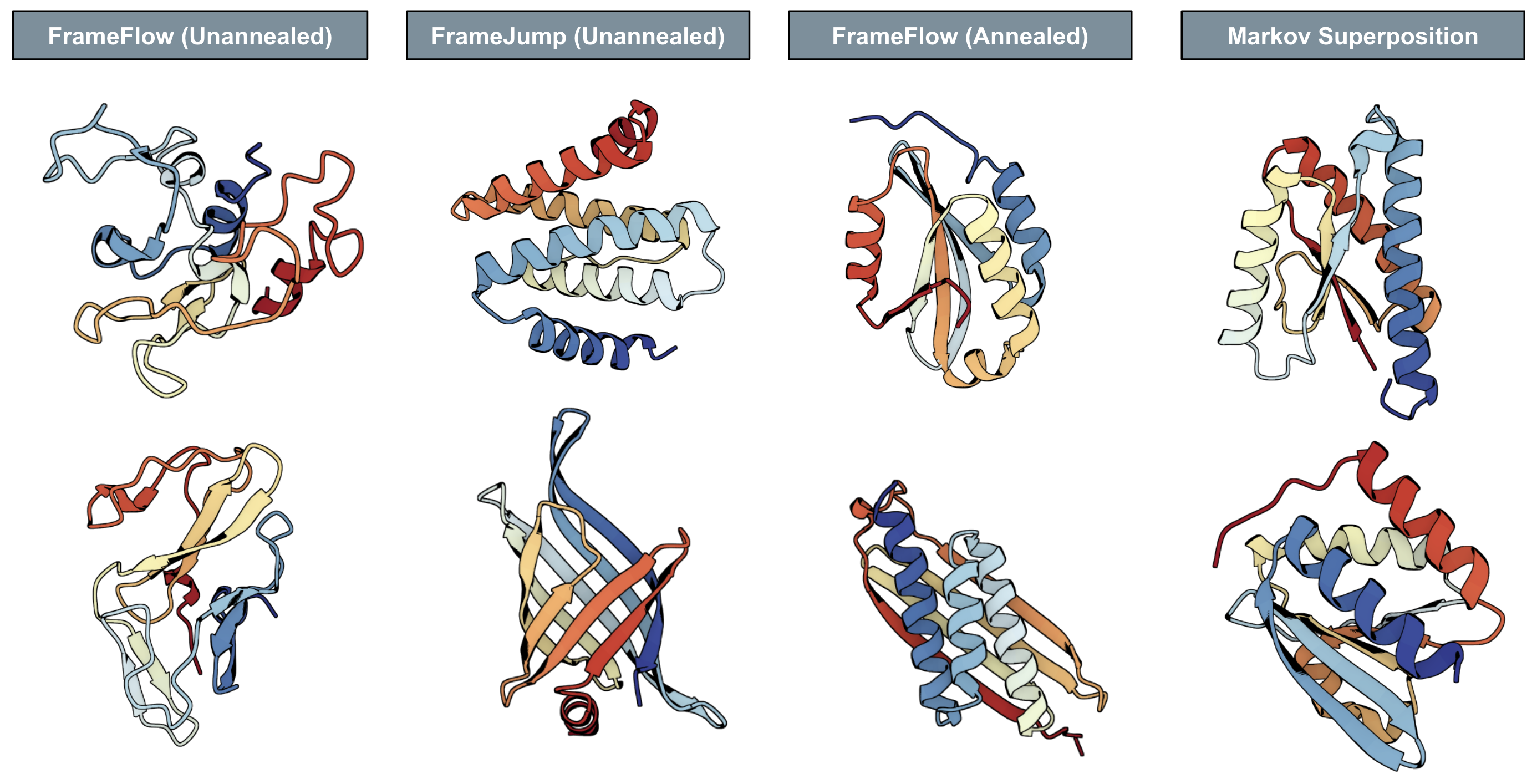
Figure 3: Examples of generated proteins for various model combinations.

Building models for arbitrary state spaces - Protein experiments. GM allows us to design models for arbitrary state spaces. To illustrate this, we repurpose FrameFlow, a state-of-the-art $SE(3)$ flow model for protein structure generation (Yim et al., 2023a; 2024) and show it can be improved using jump models. Specifically, we derive a novel solution $\mathcal{L}_{t}^{z}$ to the KFE on $S=SO(3)$ with a jump model (see sec. G.1). We then make this model multi-dimensional ($S=SO(3)^{d}$) and combine it with a flow model on $\mathbb{R}^{d}$ ($S=\mathbb{R}^{d}\times SO(3)^{d}$) using proposition 4. Using the pre-trained FrameFlow without any fine-tuning, we “pseudo-marginalize” the conditional jumps by predicting $x_{1}\in SE(3)$ and then taking a conditional step with $\mathcal{L}_{t}^{z}$. We refer to this method as FrameJump. In fig. 3, we can see examples of generated proteins. We benchmark our results by following Yim et al. (2023a) to compute the following metrics: Diversity (Div) is the proportion of unique proteins passing a protein quality check called designability, Novelty (Nov) is the average inverse similarity of each protein passing designability. Table 2 shows our results compared to FrameFlow and its precursor, FrameDiff, a $SE(3)$ diffusion model (Yim et al., 2023a). We see that FrameJump significantly outperforms FrameDiff while achieving better novelty than FrameFlow. We show combining FrameFlow and FrameJump provides the best result with improved diversity compared to only using FrameFlow. Sec. G.4 provides more experiment details. This result illustrates that decoupling the probability path from the KFE solution gives a powerful design choice - leading to improvements of models without even the need to re-train them.

Method	CIFAR10	ImageNet
DDPM (Ho et al., 2020)	$3.17$	$6.99$
VP-SDE (Song et al., 2020)	$3.01$	$6.84$
EDM (Karras et al., 2022)	$1.98$	$-$
Flow model (Euler)	$2.94$	$4.58$
Jump model (Euler)	$4.23$	$7.66$
Jump + Flow MS (Euler)	2.49	3.47
Flow model (2nd order)	$2.48$	$3.59$
Jump + Flow MS (mixed)	2.36	3.33

Table 3: Experimental results for image generation. FID scores are listed. MS=Markov superposition. Euler: euler sampling. 2nd order: 2nd order ODE sampler. Mixed: Flow uses 2nd order sampler and jump uses Euler sampling.

New models - Jump model. We next illustrate training from scratch on image generation experiments. We use the jump model defined in eq. 8. To parameterize a $1$d-kernel $Q_{t}(x^{\prime};x)$, we factorize it into functions $Q_{t}(x^{\prime};x)=\lambda_{t}(x)J_{t}(x^{\prime};x)$ where $J_{t}(x^{\prime};x)$ is probability kernel, i.e., $\int J_{t}(x^{\prime};x)dx^{\prime}=1$, and $\lambda_{t}(x)\geq 0$. We parameterize $J_{t}(x^{\prime};x)$ via bins in $1d$ normalizing it using a softmax function. Using proposition 4, we extend the model to arbitrary dimensions - which means we need to define $\lambda_{t},J_{t}$ per pixel (see app. F). We use a U-Net architecture with $n+1$ output channels where $n$ is the number of bins in $J_{t}$ and one channel is reserved for $\lambda_{t}$. We use a discretization of the loss from table 1. In app. D, we show that this corresponds to an ELBO loss. We refer to app. F for details of the model. We apply the model on CIFAR10 and the ImageNet32 (blurred faces) datasets. As jump models do not have an equivalent of classifier-free guidance, we focus on unconditional generation. A challenge for a fair comparison is that flow models have higher-order ODE samplers that can be used, while sampling for jump models in $\mathbb{R}^{d}$ is only done with Euler sampling. We ablate over this choice. As one can see in fig. 4, the jump model can generate realistic images of high quality. In table 3, one can see quantitative results of our experiments. While lacking behind current state-of-the art models, the jump model shows promising results as a first version of an unexplored class of models.

Combining models - Markov superposition. Next, we train a flow and jump model in the same architecture (i.e., just increase number of channels to $n+2$). We validate that the flow part achieves the state-of-the-art results as before. We then combine both models via a Markov superposition. As one can see in table 3, a Markov superposition of a flow and jump model boosts the performance of each other and there are synergistic effects. For Euler sampling, we see significant improvements. We can also combine 2nd order samplers for flows with Euler sampling for jumps in a “mixed” sampling method (see table 3) leading to improvements of the current SOTA by flow models. We anticipate that with further improvements of the jump model (e.g. better sampling), the effect of increased performance via Markov superposition will be even more pronounced.

10 Discussion

We introduced generator matching, a general framework for scalable generative modeling on arbitrary state spaces via Markov generators. The generator abstraction offers key insights into the fundamental equations governing Markov generative models: Generators are linear operators, the KFE is a linear equation, and many losses (Bregman divergences) are linear in the training target. Therefore, any minimization we do conditionally on a data point, implicitly minimizes the training target marginalized across a distribution of data points. These principles allowed us to unify a diversity prior generative modeling methods such as diffusion models, flow matching, or discrete diffusion models. Further, we could universally characterize the space of Markov models and loss functions. GM allows us to combine generative models of different classes on the same state space (Markov superpositions) and how to build multimodal generative models from unimodal components. Future work could further explore the design space of GM. For example, we showed how one can learn a diffusion coefficient $\sigma_{t}$ of a diffusion model. In addition, jump models on Euclidean space offer a large class of models that we could only study here in its simple instances. In addition, future work can explore better samplers or distillation to minimize computational cost during sampling. To conclude, generator matching provides both a rigorous theoretical foundation and opens up a large practical design space to advance generative modeling across a diverse range of applications.

Acknowledgments

P.H. would like to thank Yann Ollivier for his insightful comments and for sharing his mathematical expertise throughout the project. Further, P.H. would like to thank Andreas Eberle for mathematical support and advice as well as for sharing excellent teaching materials for Markov process theory. Further, we would like to thank Maurice Weiler, Ishaan Chandratreya, Alexander Sauer, and Krunoslav Lehman Pavasovic for extensive feedback on early drafts of the work. We also thank Anuroop Sriram and Daniel Severo for feedback and help along the way. Finally, we would like to thank Heli Ben-Hamu for sharing code for von Mises–Fisher distributions.

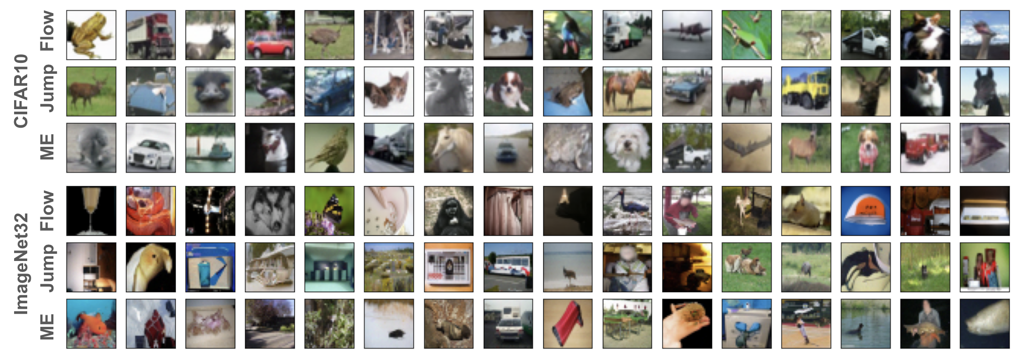
Figure 4: . Examples of generated images on CIFAR10 (top) and ImageNet32 (bottom).

Algorithm 1 Generator Matching recipe for constructing Markov generative model (theory in black, implementation in brown)

Step 0: Choose prior $p_{\text{simple}}$
Step 1: Choose $p_{t}(dx|z)$ such that
marginal $p_{0}=p_{\text{simple}}$ and $p_{1}=p_{\text{data}}$
Step 2: Find solution $\mathcal{L}_{t}^{z}$ to KFE
Step 3: Choose Bregman div. as loss
Step 4: Construct neural net $\mathcal{L}_{t}^{\theta}$
Step 5: Minimize CGM loss using $\mathcal{L}_{t}^{z}$
Step 6: Sample using Algorithm 2.

Algorithm 2 Euler sampling for $S=\mathbb{R}^{d}$

Given: $u_{t},\sigma_{t}$, $Q_{t}$, $p_{\text{simple}}$, step size $h>0$
Init: $X_{0}\sim p_{\text{simple}}$

1:for $t$ in $\text{linspace}(0,1,1/h)$ do

2:     Jump intensity $\lambda_{t}(X_{t})=\int Q_{t}(dy;X_{t})$

3:     $\bar{X}_{t+h}\sim Q_{t}(\cdot;X_{t})/\lambda_{t}(X_{t})$

4:     $m\sim\text{Bernoulli}(h\lambda_{t}(X_{t}))$, $\epsilon_{t}\sim\mathcal{N}(0,1)$

5:     $\tilde{X}_{t+h}=X_{t}+hu_{t}(X_{t})+\sqrt{h}\sigma_{t}(X_{t})\epsilon_{t}$

6:     $X_{t+h}=m\bar{X}_{t+h}+(1-m)\tilde{X}_{t+h}$

7:end for

Return: $X_{1}$

Appendix A Overview of Markov Processes and their generators

A.1 Setup and Definitions

State space. Throughout this work, we assume $(S,d)$ is a Polish metric space, i.e., $S$ is a set and there is a metric $d:S\times S\to\mathbb{R}_{\geq 0}$ defined on $S$ such that $(S,d)$ is complete (i.e., any Cauchy sequence converges) and separable (i.e., it has a countable dense subset). We endow $S$ with its Borel $\sigma$-algebra $B(S)$ and consider a set $A\subset S$ as measurable if $A\in B(S)$. Any function $f:S\to\mathbb{R}$ considered in this work is assumed to be measurable. Throughout this work, we assume that $\mathcal{T}$ is a set of functions $f:S\to\mathbb{R}$ on $S$ such two probability measures $\mu_{1},\mu_{2}$ are equal if and only if $\mathbb{E}_{x\sim\mu_{1}}[f(X_{t})]=\mathbb{E}_{x\sim\mu_{2}}[f(x)]$ for all $f\in\mathcal{T}$. We call elements in $\mathcal{T}$ test functions.

Markov process. Let $(\Omega,\mathcal{F},\mathbb{P})$ be a probability space. A Markov process $(X_{t})_{0\leq t1}$ is a collection of integrable random variables $X_{t}:\Omega\to S$ such that

Markov assumption: $$\mathbb{P}[X_{t_{n+1}}\in A|X_{t_{1}},X_{t_{2}},\dots,X_{t_{n}}]=\mathbb{P}[X_{t_{n+1}}\in A|X_{t_{n}}]$$

$$\text{for all }0\leq t_{1}<t_{2}<\dots<t_{n}<t_{n+1}\leq 1,A\subseteq S\text{ measurable}$$

We denote by $k_{t+h|t}(A|x)=\mathbb{E}[X_{t+h}\in A|X_{t}=x]$ the transition kernel of $X_{t}$.

Semigroup.

We define the action of marginals $p_{t}$ and of transition kernels $k_{t+h|t}$ on test functions $f$ as in the main paper via:

$$p_{t}\odot f =\int f(y)p_{t}(dy)=\mathbb{E}\left[f(X_{t})\right] \blacktriangleright\text{marginal action}$$ (11)

$$\left[k_{t+h|t}\odot f\right](x) =\int f(y)k_{t+h|t}(dy|x)=\mathbb{E}\left[f(X_{t+h})|X_{t}=x\right] \blacktriangleright\text{transition action}$$ (12)

where the marginal action maps each test function $f$ to a scalar $p_{t}\odot f\in\mathbb{R}$, while transition action maps a real-valued function $x\mapsto f(x)$ to a another real-valued function $x\mapsto[k_{t+h|t}\odot f](x)$. The tower property implies that $p_{t}\odot[k_{t+h|t}\odot f]=p_{t+h}\odot f$. Considering $k_{t+h|t}$ as a linear operator as above, we know by the Markov assumption and the tower property that there are two fundamental properties that hold:

$$k_{t|t}= \text{Id},\quad p_{s|u}=p_{t|u}\odot p_{s|t},\quad 0\leq u<t<s\leq 1 \blacktriangleright\text{composition}$$

$$\|p_{s|t}f\|_{\infty}\leq \|f\|_{\infty},\quad 0\leq t<s\leq 1 \blacktriangleright\text{contraction}$$

where $\|\cdot\|_{\infty}$ describes the supremum norm.

A.1.1 Definitions for time-homogeneous Markov processes

A complication in the theory we develop here is that we (need to) consider time-inhomogeneous Markov processes, while most of the mathematical theory and literature resolves around time-homogeneous Markov processes. Therefore, we first give the definitions for time-homogeneous Markov processes and then explain how this can be translated to the time-homogenous case.

A time-homogeneous Markov process is a Markov process $\bar{X}_{t}$ such that $k_{t+h|t}=k_{h|0}$ for all $t,h\geq 0$ - i.e. the evolution is constant in time. This implies the semigroup property

$$k_{t|0}=\text{Id},\quad k_{s|0}\odot k_{t|0}=k_{s+t|0}$$

Let $C_{0}(S)$ be the space of continuous functions $f:S\to\mathbb{R}$ that vanish at infinity, i.e. for all $\epsilon>0$ there exists a compact set $K\subset S$ such that $|f(x)|<\epsilon$ for all $x\in S\setminus K$.

Feller process.

We call $\bar{X}_{t}$ a Feller process if it holds that

1. Operators on continuous functions: For any $f\in C_{0}(S)$ and $t\geq 0$, also $k_{t|0}f\in C_{0}(S)$.

2. Strong continuity: For any $f\in C_{0}(S)$:

   $$\lim\limits_{t\downarrow 0}\|k_{t|0}f-f\|_{\infty}=0$$

Generator.

We define the generator $\mathcal{L}$ of a Feller process $\bar{X}_{t}$ as follows: for any $f\in C_{0}(S)$ such that the limit

$$\lim\limits_{t\downarrow 0}\frac{k_{t|0}f-f}{t}\to\mathcal{L}f$$

exists uniformly in $S$ (i.e., in $\|\cdot\|_{\infty}$) and we define $\mathcal{L}f$ as the limit above. We define the core $D(\mathcal{L})$ as all $f$ for which that limit exists. It holds that $D(\mathcal{L})$ is a dense subspace of $C_{0}(S)$ (Pazy, 2012) and $\mathcal{L}$ is a linear operator.

A.1.2 Definitions for time-inhomogeneous Markov processes

For a general time-inhomogeneous Markov process $X_{t}$, one can extend the definitions to a two-parameter semigroup, see (Rüschendorf et al., 2016) for example. Another approach is to simply consider the corresponding time-homogeneous Markov process $\bar{X}_{t}=(X_{t},t)$ on extended state space $S\times[0,1]$. The transition kernel on extended state space is then given for $A\subset S\times[0,1]$ via:

$$\bar{p}_{h|0}(A,(x,t))=k_{t+h|t}(A_{t+h},x),\quad A_{t+h}:=\{y|(y,t+h)\in A\}$$

and the action is given via

$$\bar{p}_{h|0}f(x,t)=\mathbb{E}[f(X_{t+h},t+h)|X_{t}=x]$$

Feller process.

The Feller assumption is equivalent to:

1. Operators on continuous functions: For any $f\in C_{0}(S\times[0,1])$ and $t\geq 0$, also $k_{t|0}f\in C_{0}(S\times[0,1])$.

2. Strong continuity: For any $f\in C_{0}(S\times[0,1])$:

   $$\lim\limits_{t\downarrow 0}\|k_{t|0}f-f\|_{\infty}=0$$

   where here the supremum norm $\|\cdot\|_{\infty}$ is taken across $S$ and time $[0,1]$.

Time-dependent generator.

In the above case, we can reshape the generator via

$$\mathcal{L}f(x,t)= \lim\limits_{h\to 0}\frac{\mathbb{E}[f(X_{t+h},t+h)-f(X_{t},t)|X_{t}=x]}{h}$$

$$= \lim\limits_{h\to 0}\frac{\mathbb{E}[f(X_{t+h},t+h)-f(X_{t},t+h)+f(X_{t},t+h)-f(X_{t},t)|X_{t}=x]}{h}$$

$$= \lim\limits_{h\to 0}\left[\frac{\mathbb{E}[f(X_{t+h},t+h)-f(X_{t},t+h)|X_{t}=x}{h}\right]+\lim\limits_{h\to 0}\frac{f(x,t+h)-f(x,t)}{h}$$

$$= \underbrace{\lim\limits_{h\to 0}\left[\frac{\mathbb{E}[f(X_{t+h},t+h)-f(X_{t},t+h)|X_{t}=x]}{h}\right]}_{=:\mathcal{L}_{t}f^{t}(x)}+\partial_{t}f(x,t)$$

$$= \mathcal{L}_{t}f^{t}(x)+\partial_{t}f(x,t)$$

where $f^{t}:S\to\mathbb{R},x\mapsto f(x,t)$ describes the restriction of $f$ on $S$ and we defined the time-dependent generator $\mathcal{L}_{t}$ as an operator acting on spatial components, i.e. functions in $C_{0}(S)$, via

$$\mathcal{L}_{t}g(x):=\frac{\mathbb{E}[g(X_{t+h})-g(X_{t})|X_{t}=x]}{h}$$ (13)

for any $g:S\to\mathbb{R}$ such that the limit exists. Note that however that when we define the time-dependent generator $\mathcal{L}_{t}f$, we also need to specify the direction operator $\partial_{t}$ (i.e. in what direction of time it goes). This is always implicitly assumed. Further, we remark that in the above derivation, we have assumed that $t\mapsto\mathcal{L}_{t}f^{t}$ is continuous (in supremum norm) in $t$ for any function in the domain of $\mathcal{L}_{t}$. We will state this now again.

A.2 Regularity Assumptions.

Throughout this work, we make the following regularity assumptions:

1. Assumption on semigroup: The Markov process $X_{t}$ is a Feller process in the sense defined in sec. A.1.2.

2. Assumption on sample paths: In every time interval $[s,t]$, the expected number of discontinuities of $t\mapsto X_{t}$ is finite.

3. Assumptions on test functions: There exists a subspace of test functions $\mathcal{T}$ that is dense in $C_{0}(S)$ such that $\mathcal{T}\subset\text{dom}(\mathcal{L}_{t})$ and the function $t\mapsto\mathcal{L}_{t}f$ is continuous for any $f\in\mathcal{T}$. Further, two probability distributions $\mu_{1},\mu_{2}$ on $S$ are equal if and only if for all $f\in\mathcal{T}$ it holds that $\mathbb{E}_{x\sim\mu_{1}}[f(x)]=\mathbb{E}_{x\sim\mu_{2}}[f(x)]$.

4. Assumptions on probability path: Any probability path $(p_{t})_{0\leq t\leq 1}$ considered fulfils that the function $t\mapsto p_{t}\odot f$ is continuous in $t$ for all $f\in\mathcal{T}$.

5. KFE is sufficient to check probability path: Let $(p_{t})_{0\leq t\leq 1}$ be a probability path on $S$. Then:

   $$X_{0}\sim p_{0}\quad$$ (start with right initial distribution)

   $$\partial_{t}[p_{t}\odot f]= p_{t}\odot\mathcal{L}_{t}f\text{ for all }f\in\mathcal{T}$$ (fulfil KFE)

   $$\Rightarrow X_{t}\sim p_{t}\text{ for all }0\leq t\leq 1 \text{ (marginals of }X_{t}\text{ are given by }p_{t})$$

   i.e. if $X_{t}$ is initialized with the right initial distribution, its marginals will be given by $p_{t}$.

Remark regarding assumption 5.

We note that assumption 5 is true under relatively weak assumptions and there is a diversity of mathematical literature on showing uniqueness of the solution of the KFE in $p_{t}$ for different settings. However, to the best of our knowledge, there is no known result that states regularity assumptions for general state spaces and Markov processes, which is why simply state it here as an assumption. For the machine learning practitioner, this assumption holds for any state space of interest. To illustrate this, we point the rich sources in the mathematical literature that show uniqueness that list the regularity assumptions for specific spaces and classes of Markov processes:

1. Flows in $\mathbb{R}^{d}$ and manifolds: (Villani et al., 2009, Mass conservation formula, page 15), (DiPerna & Lions, 1989), (Ambrosio, 2004)

2. Diffusion in $\mathbb{R}^{d}$ and manifolds: (Villani et al., 2009, Diffusion theorem, page 16)

3. General Ito-SDEs in $\mathbb{R}^{d}$: (Figalli, 2008, Theorem 1.3 and 1.4), (Kurtz, 2011, Corollary 1.3), (Bogachev et al., 2022)

4. Discrete state spaces: Here, the KFE is a linear ODE, which has a unique solution under the assumption that the coefficients are continuous.

A.3 Adoint KFE

The version of the KFE in eq. 6 determines the evolution of expectations of test functions $f$. This is necessary if we use probability distributions that do not have a density. If a density exists, a more familiar version of the KFE can be used that directly prescribe the change of the probability densities. To present it, we introduce the adjoint generator ${\mathcal{L}}_{t}^{*}$, which acts on probability densities $p_{t}(x)$, namely $[{\mathcal{L}}_{t}^{*}p_{t}](x)$ is implicitly defined by the identity

$$p_{t}\odot[{\mathcal{L}}_{t}f]=[{\mathcal{L}}_{t}^{*}p_{t}]\odot f,\quad\forall f\in{\mathcal{T}}.$$ (14)

Now, equation 14 applied to the KFE (equation 6) we get

$$\int\partial_{t}p_{t}(x)f(x)dx$$

$$= \partial_{t}\int p_{t}(x)f(x)dx$$

$$= \partial_{t}[p_{t}\odot f]$$

$$= p_{t}\odot[\mathcal{L}_{t}f]$$

$$= [{\mathcal{L}}_{t}^{*}p_{t}]\odot f$$

$$= \int[{\mathcal{L}}_{t}^{*}p_{t}](x)f(x)dx$$

where "$dx$" denotes the integration with respect to some reference measure on $S$. As this holds for all test functions $f$, we can conclude that

$$\partial_{t}p_{t}(x)=[{\mathcal{L}}_{t}^{*}p_{t}](x)\text{ for all }x\in S\qquad\blacktriangleright\text{Adjoint KFE}$$ (15)

which is an equivalent version of the KFE that we call adjoint KFE. In this form, the KFE generalizes many famous equations used to develop generative models such as the Continuity Equation or the Fokker-Planck Equation (Song et al., 2020; Lipman et al., 2022) (see table 1). Whenever a probability density exists, we use the adjoint KFE. We will derive several examples of adjoint generators and adjoint KFEs in sec. A.4.

A.4 Properties of important Markov processes (derivations for table 1)

In this section, we include the definition of important classes of Markov processes and their properties including their generators.

A.4.1 Flows

Definition.

Let $S=\mathbb{R}^{d}$ and $u:\mathbb{R}^{d}\times\mathbb{R}\to\mathbb{R}^{d},(x,t)\mapsto u_{t}(x)$ be a time-dependent vector field. Then a flow $\phi_{t,s}(x)$ is the solution to the ODE:

$$\frac{d}{dt}\phi_{t,s}(x)=u_{t}(\phi_{t,s}(x),t),\quad\phi_{s,s}(x)=x$$

It is clear that $\phi_{t,s}$ is a deterministic Markov transition kernel $p_{t|s}$, i.e. $p_{t|s}(\cdot;x)$ is a delta distribution for every $x\in\mathbb{R}^{d}$. Euler sampling of the ODE corresponds to

$$X_{t+h}=X_{t}+hu_{t}(X_{t})+o(h)$$

Generator.

Let $\mathcal{T}=C_{c}^{\infty}(\mathbb{R}^{d})$ be the space of infinitely differentiable and smooth functions with compact support (test function in $\mathbb{R}^{d}$). Then we can compute the generator via

$$[{\mathcal{L}}_{t}f](x) =\lim_{h\rightarrow 0}\frac{\mathbb{E}\left[f(X_{t}+hu_{t}(X_{t})+o(h))|X_{t}=x\right]-f(x)}{h}$$

$$=\lim_{h\rightarrow 0}\frac{h\nabla f(x)^{T}u_{t}(x)+o(h)}{h}=\nabla f(x)^{T}u_{t}(x),$$

where we used a first-order Taylor approximation and the limit is uniform by the fact that $f$ is in $C_{c}^{\infty}(\mathbb{R}^{d})$.

Adjoint and adjoint KFE.

Let’s assume that $p_{t}$ has a density $p_{t}(x)$ that is bounded. We can compute the adjoint generator $\mathcal{L}_{t}^{*}$ via

$$p_{t}\odot[\mathcal{L}_{t}f]= \mathbb{E}_{x\sim p_{t}}[\mathcal{L}_{t}f(x)]$$

$$= \int\mathcal{L}_{t}f(x)p_{t}(x)dx$$

$$= \int\nabla f(x)^{T}u_{t}(x)p_{t}(x)dx$$

$$= \int f(x)[-\nabla\cdot[u_{t}(x)p_{t}(x)]]dx$$

$$= \int f(x)[{\mathcal{L}}_{t}^{*}p_{t}](x)dx$$

by partial integration. Therefore, the adjoint generator is given by ${\mathcal{L}}_{t}^{*}p_{t}=-\nabla\cdot[u_{t}(x)p_{t}(x)]$. Using the adjoint KFE, we get the well-known continuity equation

$$\partial_{t}p_{t}(x)=-\nabla\cdot[u_{t}p_{t}](x)$$

A.4.2 Diffusion

Definition.

Let $S=\mathbb{R}^{d}$ and $\sigma_{t}:\mathbb{R}^{d}\times\mathbb{R}\to\mathbb{R}^{d\times d},(x,t)\mapsto\sigma_{t}(x)$ be a time-dependent function mapping to symmetric positive semi-definite matrices $\sigma_{t}$ in a continuous fashion. A diffusion process with diffusion coefficient $\sigma_{t}$ is defined via the infinitesimal sampling procedure:

$$X_{t+h}=X_{t}+\sqrt{h}\sigma_{t}(X_{t})\epsilon_{t}$$

where $\epsilon_{t}\sim\mathcal{N}(0,I)$. For a more formal definition, see (Oksendal, 2013).

Generator.

Let $\mathcal{T}=C_{c}^{\infty}(\mathbb{R}^{d})$ be the space of infinitely differentiable and smooth functions with compact support (test function in $\mathbb{R}^{d}$). Then we can compute the generator via

$$[{\mathcal{L}}_{t}f](x) =\lim_{h\rightarrow 0}\frac{\mathbb{E}\left[f(X_{t}+\sqrt{h}\sigma_{t}(X_{t})\epsilon_{t}+o(h))|X_{t}=x\right]-f(x)}{h}$$

$$=\lim_{h\rightarrow 0}\frac{\mathbb{E}[f(x)+\nabla f(x)^{T}\sqrt{h}\sigma_{t}(x)\epsilon_{t}+\frac{1}{2}h[\sigma_{t}(x)\epsilon_{t}]^{T}\nabla^{2}f(x)[\sigma_{t}(x)\epsilon_{t}]-f(x)]}{h}$$

$$=\lim_{h\rightarrow 0}\frac{\nabla f(x)^{T}\sqrt{h}\sigma_{t}(x)\mathbb{E}[\epsilon_{t}]+\mathbb{E}[\frac{1}{2}h[\sigma_{t}(x)\epsilon_{t}]^{T}\nabla^{2}f(x)[\sigma_{t}(x)\epsilon_{t}]]}{h}$$

$$=\frac{1}{2}\mathbb{E}[\epsilon_{t}^{T}[\sigma_{t}(x)]^{T}\nabla^{2}f(x)[\sigma_{t}(x)]\epsilon_{t}]]$$

$$=\frac{1}{2}\text{Trace}\left(\sigma_{t}(x)^{T}\nabla^{2}f(x)\sigma_{t}(x)\right)$$

$$=\frac{1}{2}\text{Trace}[\sigma_{t}(x)\sigma_{t}(x)^{T}\nabla^{2}f(x)]$$

$$=\frac{1}{2}\sigma_{t}^{2}(x)\cdot\nabla^{2}f(x)$$

where we used a 2nd order Taylor approximation (2nd order because $\mathbb{E}[\|\sqrt{h}\epsilon_{t}\|^{2}]\propto h$) and the symmetry of $\sigma_{t}^{2}$.

Adjoint and adjoint KFE.

Let’s assume that $p_{t}$ has a density $p_{t}(x)$. We can compute the adjoint generator $\mathcal{L}_{t}^{*}$ via

$$p_{t}\odot[\mathcal{L}_{t}f]= \mathbb{E}_{x\sim p_{t}}[\mathcal{L}_{t}f(x)]$$

$$= \int\mathcal{L}_{t}f(x)p_{t}(x)dx$$

$$= \frac{1}{2}\int\sigma_{t}^{2}(x)\cdot\nabla^{2}f(x)p_{t}(x)dx$$

$$= \frac{1}{2}\int f(x)\nabla^{2}\cdot[\sigma_{t}^{2}p_{t}](x)dx$$

$$= \int f(x)[\mathcal{L}_{t}^{*}p_{t}](x)dx$$

by partial integration. Using the fact that this holds for all test functions, we can convert the KFE to the adjoint KFE recovering the well-known Fokker-Planck equation

$$\partial_{t}p_{t}(x)=\nabla^{2}\cdot[\sigma_{t}^{2}p_{t}](x)$$

A.4.3 Jumps

Let us assume that we consider a jump process defined by a time-dependent kernel $Q_{t}(dy;x)$, i.e. for every $0\leq t\leq 1$ and every $x\in S$, $Q_{t}(dy;x)$ is a positive measure over $S\setminus\{x\}$. The idea of a jump process is that the total volume assigned to $S$

$$\lambda_{t}(x)=\int Q_{t}(dy;x)$$

gives the jump intensity, i.e. the infinitesimal likelihood of jumping. Further, if $\lambda_{t}(x)>0$, we can assign a jump distribution by normalizing $Q_{t}$ to a probability kernel

$$J_{t}(dy;x)=\frac{Q_{t}(dy;x)}{\lambda_{t}(x)}$$

The infinitesimal sampling procedure is as follows:

$$X_{t+h}=\begin{cases}X_{t}&\text{with probability }1-h\lambda_{t}(X_{t})\\ \sim J_{t}(dy;X_{t})&\text{with probability }h\lambda_{t}(X_{t})\end{cases}$$

We derive the generator here in an informal way. For a rigorous treatment of jump processes, see for example (Davis, 1984). Up to $o(h)$-approximation error, the generator is then given by

$$\mathcal{L}_{t}f(x)= \lim\limits_{h\to 0}\frac{\mathbb{E}[f(X_{t+h})-f(X_{t})|X_{t}=x]}{h}$$

$$= \lim\limits_{h\to 0}\frac{\mathbb{E}[f(X_{t+h})-f(X_{t})|X_{t}=x,\text{Jump in }[t,t+h)]\mathbb{P}[\text{Jump in }[t,t+h)]}{h}$$

$$+\lim\limits_{h\to 0}\underbrace{\frac{\mathbb{E}[f(X_{t+h})-f(X_{t})|X_{t}=x,\text{No jump in }[t,t+h)]\mathbb{P}[\text{No jump in }[t,t+h)]}{h}}_{=0}$$

$$= \lim\limits_{h\to 0}\frac{\mathbb{E}_{y\sim J_{t}(dy;x)}\left[f(y)-f(x)\right]h\lambda_{t}(x)}{h}$$

$$= \mathbb{E}_{y\sim J_{t}(dy;x)}\left[f(y)-f(x)\right]\lambda_{t}(x)$$

$$= \int f(y)-f(x)Q_{t}(dy;x)$$

where we have used that if $X_{t}$ does not jump in $[t,t+h]$, then $X_{t+h}=X_{t}$.

Adjoint and adjoint KFE.

Let’s assume that $p_{t}$ has a density $p_{t}(x)$ and that the jump measures $Q_{t}(dy;x)$ is given via a kernel $Q_{t}:S\times S\to\mathbb{R}_{\geq 0},(y,x)\mapsto Q_{t}(y;x)$ such that

$$\int f(y)Q_{t}(dy;x)=\int f(y)Q_{t}(y;x)dy$$

where $dy$ denotes the integration with respect to some reference measure on $S$ (e.g. the Lebesgue measure on $\mathbb{R}^{d}$ or just summation on $S$ discrete). Then we can derive the adjoint generator as follows:

$$p_{t}\odot\mathcal{L}_{t}f(x)= \int\int(f(y)-f(x))Q_{t}(y;x)dyp_{t}(x)dx$$

$$= \int\int f(y)Q_{t}(y;x)p_{t}(x)dydx-\int\int f(x)Q_{t}(y;x)p_{t}(x)dydx$$

$$= \int\int f(x)Q_{t}(x;y)p_{t}(y)dydx-\int\int f(x)Q_{t}(y;x)p_{t}(x)dydx$$

$$= \int f(x)\underbrace{\left[\int Q_{t}(x;y)p_{t}(y)-Q_{t}(y;x)p_{t}(x)dy\right]}_{=:\mathcal{L}_{t}^{*}p_{t}}dx$$

where we have seen that $\mathcal{L}_{t}^{*}$ describes the adjoint generator. With this, we get the jump continuity equation as adjoint KFE

$$\partial_{t}p_{t}(x)=\int\underbrace{Q_{t}(x;y)p_{t}(y)}_{\text{inflow}}-\underbrace{Q_{t}(y;x)p_{t}(x)}_{=\text{outflow}}dy$$

A.4.4 Continuous-time Markov chain (CTMC)

Let us consider a continuous-time Markov chain $X_{t}$ on a discrete space $S$ with $|S|<\infty$. We define this to be a jump process as defined in sec. A.4.3. However, we can find a convenient parameterization for the jump process. Specifically, we can convert integrals into sums and see that there is a jump kernel $Q_{t}\in\mathbb{R}^{S\times S}_{\geq 0}$ given such that for all $x\in S$ it holds that

$$\mathcal{L}_{t}f(x)= \sum\limits_{y\in S}[f(y)-f(x)]Q_{t}(y;x)=\sum\limits_{y\neq x}[f(y)-f(x)]Q_{t}(y;x)$$

A natural convention people follow is to set $Q_{t}(x;x)=-\sum\limits_{y\neq x}Q_{t}(y;x)$. This gives us the rate of staying at $x$ (However, not that $Q_{t}(y;x)$ does not describe a kernel of a positive measure anymore.) With this constraint, we get

$$\mathcal{L}_{t}f(x)=\sum\limits_{y\in S}f(y)Q_{t}(y;x)=f^{T}Q_{t}$$

where we consider $f=(f(x))_{x\in S}$ as a row vector. The adjoint is simply given by the adjoint multiplication $p_{t}\mapsto Q_{t}p_{t}$ and we get that the adjoint KFE is given by

$$\partial_{t}p_{t}(x)=\sum\limits_{y\in S}Q_{t}(x;y)p_{t}(y)$$

To sample the next time step given $X_{t}=x$, we get

$$X_{t+h}= \begin{cases}\sim\frac{Q_{t}(y;x)}{\sum\limits_{y\neq x}Q_{t}(y;x)}&\text{with probability }h\sum\limits_{y\neq x}Q_{t}(y;x)\\ x&\text{with probability }1-h\sum\limits_{y\neq x}Q_{t}(y;x)\\ \end{cases}$$

$$= \begin{cases}\sim\frac{Q_{t}(y;x)}{\sum\limits_{y\neq x}Q_{t}(y;x)}&\text{with probability }h\sum\limits_{y\neq x}Q_{t}(y;x)\\ x&\text{with probability }1+hQ_{t}(x;x)\\ \end{cases}$$

$$= \begin{cases}y&\text{with probability }hQ_{t}(y;x)\text{ (for all }y\in S)\\ x&\text{with probability }1+hQ_{t}(x;x)\\ \end{cases}$$

$$\sim (I+hQ_{t})(\cdot;x)$$

where we simply sample from the stochastic matrix $I+hQ_{t}$ (a matrix whose columns sum to $1$).

A.5 Linear parameterization of generators

We describe here what we understand under a linear parameterization of a generator. This is the basis for parameterizing a generator in a neural network that can be implemented in a computer. For simplicity, we fix a $t\in[0,1]$. As before, $\mathcal{T}$ be the space of test functions and $B(S)$ be the space of bounded functions on $S$. Then the space $A(\mathcal{T}):=\{\mathcal{L}:\mathcal{T}\to B(S)|\mathcal{L}\text{ is linear}\}$ of linear operators on $\mathcal{T}$ is itself again a vector space. Let $W\subset A(\mathcal{T})$ be a subspace. Then a linear parameterization of $W$ is given by 2 components: (1) a convex closed set $\Omega\subset V$ that is a subset of a vector space with an inner product $\left\langle\cdot,\cdot\right\rangle_{V}$ and (2) a linear operator $D:\mathcal{T}\to C(S;V)$ such that every $\mathcal{L}_{t}\in W$ can be written as

$$\mathcal{L}_{t}f(x)=\left\langle\mathcal{D}f(x);F_{t}(x)\right\rangle_{V}$$ (16)

for a continuous function $F_{t}:S\to\Omega$. We list several examples to make this abstract definition more concrete.

1. Flows in $S=\mathbb{R}^{d}$: $\mathcal{T}=C_{c}^{\infty}(\mathbb{R}^{d})$ and $\Omega=V=\mathbb{R}^{d}$. Let $W$ be the space of linear operators given via generators of flows, i.e.

   $$\mathcal{L}_{t}f=\nabla f^{T}u_{t},\quad u_{t}:\mathbb{R}^{d}\to\mathbb{R}^{d}$$

   Setting $\mathcal{D}f=\nabla f$ and $F_{t}=u_{t}$ we recover the shape of eq. 16.

2. Diffusion in $S=\mathbb{R}^{d}$: $\mathcal{T}=C_{c}^{\infty}(\mathbb{R}^{d})$ and $\Omega=S_{d}^{++}\subset\mathbb{R}^{d\times d}=V$, where $S_{d}^{++}$ denotes the set of all positive semi-definite matrices. Let $W$ is the space of linear operators given via generators of diffusion, i.e.

   $$\mathcal{L}_{t}f=\nabla^{2}f\cdot\sigma_{t}^{2},\quad\sigma_{t}:\mathbb{R}^{d}\to S_{d}^{++}$$

   Setting $\mathcal{D}f=\nabla^{2}f$ and $F_{t}=\sigma_{t}^{2}$ we recover the shape of eq. 16.

3. Jumps in $S=\mathbb{R}^{d}$: $\mathcal{T}=C_{c}^{\infty}(\mathbb{R}^{d})$ and $\Omega=\{a:\mathbb{R}^{d}\to\mathbb{R}_{\geq 0},a\text{ continuous}\}\subset C^{1}(\mathbb{R}^{d},\mathbb{R})=V$. On $V$, a dot product is defined via $\left\langle a,b\right\rangle_{V}=\int a(x)b(x)dx$. Let $W$ be the space of linear operators given via generators of jumps, i.e.

   $$\mathcal{L}_{t}f(x)=\int f(y)-f(x)Q_{t}(y;x)dy=\left\langle Df(x),Q_{t}(\cdot;x)\right\rangle_{V}$$

   where we set $\mathcal{D}f(x)$ as the function $y\mapsto f(y)-f(x)$. Setting $F_{t}=Q_{t}$ we recover the shape of eq. 16.

4. Continuous-time Markov chains: Let $S$ be discrete and $Q_{t}\in\mathbb{R}^{S\times S}$ be a rate matrix of a continuous-time Markov chain. Then for any $f\in\mathbb{R}^{S}$

   $$\mathcal{L}_{t}f(x)=f^{T}Q_{t}(\cdot;x)=\left\langle f,Q_{t}(\cdot;x)\right\rangle_{V}$$

   where $V=\mathbb{R}^{S}$ and $Df=f$ and $\left\langle\cdot,\cdot\right\rangle_{V}$ is the standard Euclidean dot product. With this, we recover the shape of eq. 16.

Appendix B Sampling with universal representation (alg. 2)

In alg. 2, we summarize a sampling procedure to sample a generator for $S=\mathbb{R}^{d}$ with universal representation described in theorem 1. We briefly want to derive that alg. 2 is in fact a method a sampling procedure that simulates a Markov process with the correct generator up to $o(h)$ approximation error. Let us assume that $X_{t}$ is a Markov process that is obtained by sampling as in alg. 2 (limit process for $h\to 0$). Then its generator is given via:

$$\mathcal{L}_{t}f(x)= \lim\limits_{h\to 0}\frac{1}{h}\left(\mathbb{E}[f(X_{t+h})-f(X_{t})|X_{t}=x]\right)$$

$$= \lim\limits_{h\to 0}\frac{\mathbb{E}[f(X_{t+h})-f(X_{t})|X_{t}=x,\text{Jump in }[t,t+h)]\mathbb{P}[\text{Jump in }[t,t+h)]}{h}$$

$$+\lim\limits_{h\to 0}\underbrace{\frac{\mathbb{E}[f(X_{t+h})-f(X_{t})|X_{t}=x,\text{No jump in }[t,t+h)]\mathbb{P}[\text{No jump in }[t,t+h)]}{h}}_{=0}$$

$$= \lim\limits_{h\to 0}\frac{\mathbb{E}_{y\sim Q_{t}(dy;x)/\lambda_{t}(x)}[f(y)-f(x)]h\lambda_{t}(x)}{h}$$

$$+\lim\limits_{h\to 0}\frac{[\mathbb{E}[f(X_{t}+hu_{t}(X_{t})+\sqrt{h}\sigma_{t}(X_{t})\epsilon_{t})-f(X_{t})|X_{t}=x,\text{No jump in }[t,t+h)]](1-h\lambda_{t}(x))}{h}$$

$$= \int f(y)-f(x)Q_{t}(dy;x)$$

$$+\lim\limits_{h\to 0}\frac{\mathbb{E}[f(X_{t}+hu_{t}(X_{t})+\sqrt{h}\sigma_{t}(X_{t})\epsilon_{t})-f(X_{t})|X_{t}=x,\text{No jump in }[t,t+h)]]}{h}$$

$$= \int f(y)-f(x)Q_{t}(dy;x)$$

$$+\lim\limits_{h\to 0}\frac{\mathbb{E}[h\nabla f(x)^{T}[u_{t}(X_{t})+\sqrt{h}\sigma_{t}(X_{t})\epsilon_{t})]+\frac{1}{2}h^{2}[u_{t}(X_{t})+\sqrt{h}\sigma_{t}(X_{t})\epsilon_{t})]^{T}\nabla^{2}f(x)[u_{t}(X_{t})+\sqrt{h}\sigma_{t}(X_{t})\epsilon_{t})]]}{h}$$

$$= \int f(y)-f(x)Q_{t}(dy;x)$$

$$+\nabla f(x)^{T}u_{t}(x)+\lim\limits_{h\to 0}\frac{\mathbb{E}[\frac{1}{2}[\sigma_{t}(X_{t})\epsilon_{t})]^{T}\nabla^{2}f(x)[\sigma_{t}(X_{t})\epsilon_{t})]]}{h}$$

$$= \int f(y)-f(x)Q_{t}(dy;x)+\nabla f(x)^{T}u_{t}(x)+\frac{1}{2}\text{Trace}\left[\sigma_{t}(X_{t})\nabla^{2}f(x)\sigma_{t}(X_{t})\right]$$

$$= \int f(y)-f(x)Q_{t}(dy;x)+\nabla f(x)^{T}u_{t}(x)+\frac{1}{2}\sigma_{t}^{2}(X_{t})\cdot\nabla^{2}f(x)$$

This finishes the proof.

Appendix C Proofs

C.1 Proof of theorem 1

Let $(X_{t})_{0\leq t\leq 1}$ be a continuous-time Markov process. For now, we assume that $X_{t}$ is time-homogeneous. Let $\mathcal{L}$ be the generator of $X_{t}$ defined via

$$\mathcal{L}f(x)= \lim\limits_{h\to 0}\frac{\mathbb{E}[f(X_{t+h})-f(X_{t})|X_{t}=x]}{h}$$

We know that $\mathcal{L}$ has the following property:

$$f(x)=0,f\geq 0\quad\Rightarrow\quad\mathcal{L}f(x)\geq 0\quad(\text{``almost positive''})$$

An operator having the above property is called almost positive. The theory of almost positive operators is well-established. Specifically, we can use universal representations of almost positive operators as established in (von Waldenfels, 1965, Satz 1). Related theorems can be found in (Courrege, 1965) for characterizing differential operators satisfying the absolute maximum principle (that is closely related to the almost positive principle) and in weaker form for Markov processes (Feller, 1955). Here we use (von Waldenfels, 1965, Satz 1). Specifically, we know that $\mathcal{L}$ must have the form

$$\mathcal{L}f(x)= -c(x)f(x)+u(x)^{T}\nabla f(x)+\frac{1}{2}\sigma^{2}(x)\cdot\nabla^{2}f(x)$$

$$+\int\limits_{y\neq x}\left[f(y)-f(x)-y^{T}\nabla f(x)\mathbf{1}_{\|y-x\|<1}\right]Q(dy;x)$$

where $c(x)\geq 0,u(x)\in\mathbb{R}^{d}$ are continuous functions and $\sigma^{2}(x)$ is a positive semi-definite matrix continuous in $x$. For every $x$, $Q(dy;x)$ is a measure on $\mathbb{R}^{d}\setminus\{x\}$. The term $c(x)$ corresponds to a process that is “dying”. As we assume that our process runs from $t=0$ to $t=1$, we can drop $c(x)$. Further, using the assumption that there only exists a finite number of discontinuities (see sec. A.2), we can discard the term $y^{T}\nabla f(x)\mathbf{1}_{\|y-x\|<1}$ (alternatively, one can redefine the drift to $\bar{u}(x)=u(x)-\int y\mathbf{1}_{\|y-x\|<1}Q(dy;x)$). Therefore, we can rewrite the above formula as:

$$\mathcal{L}f= u(x)^{T}\nabla f(x)+\frac{1}{2}\sigma^{2}(x)\cdot\nabla^{2}f(x)+\int\limits_{y\neq x}f(y)-f(x)Q(dy;x)$$

C.2 Time-inhomogenous case

Let $(X_{t})_{0\leq t\leq 1}$ be a continuous-time Markov process. Now, we allow $X_{t}$ to be time-inhomogenous. To make it time-homogenous, we define $\bar{X}_{t}=(X_{t},t)$. Let $\bar{\mathcal{L}}$ be the generator of $\bar{X}_{t}$. Then for a test function $f:\mathbb{R}^{d}\times\mathbb{R}\to\mathbb{R}$ we get

$$\bar{\mathcal{L}}f= \bar{u}(x,t)^{T}\nabla_{x,t}f(x,t)+\frac{1}{2}\bar{\sigma^{2}}(x,t)\cdot\nabla^{2}_{x,t}f(x,t)+\int\limits f(y,s)-f(x,s)Q(dy,ds;x,t)$$

where $\bar{u},\bar{\sigma}^{2},Q_{t}$ are operators over the extended space $\mathbb{R}^{d}\times\mathbb{R}$, i.e. $\bar{u}(x,t)=(\bar{u}_{x}(x,t),\bar{u}_{t}(x,t))$ and

$$\bar{\sigma}(x,t)=\begin{pmatrix}\bar{\sigma}_{x,x}(x,t)&\bar{\sigma}_{x,t}(x,t)\\ \bar{\sigma}_{t,x}(x,t)&\bar{\sigma}_{t,t}(x,t)\end{pmatrix}$$

However, note that since marginal process in $t$ is deterministic and has derivative one, it must necessarily hold (by uniqueness of the representation) that $\bar{u}_{t}(x,t)=1$ and $\bar{\sigma}^{2}(x,t)_{t,x}=\bar{\sigma}^{2}(x,t)_{x,t}=\bar{\sigma}^{2}(x,t)_{t,t}=0$ and $Q(\cdot,\cdot;x,t)$ is supported over $\mathbb{R}^{d}\times\{t\}$ - i.e. is a time-dependent kernel $Q_{t}(dy;x)$. Therefore, we can rewrite the above equation as:

$$\bar{\mathcal{L}}f= \frac{\partial}{\partial t}f(x,t)+u_{t}(x)^{T}\nabla_{x}f(x,t)+\frac{1}{2}\sigma^{2}_{t}(x)\cdot\nabla^{2}_{x}f(x,t)+\int\limits f(y,t)-f(x,t)Q_{t}(dy;x)$$

Rewriting $\bar{\mathcal{L}}$ as a time-dependent generator $\mathcal{L}_{t}$ (see sec. A.2), we get for a time-independent test function $f:\mathbb{R}^{d}\to\mathbb{R}$

$$\mathcal{L}_{t}f= u_{t}(x)^{T}\nabla_{x}f(x)+\frac{1}{2}\sigma^{2}_{t}(x)\cdot\nabla^{2}_{x}f(x)+\int\limits f(y)-f(x)Q_{t}(dy;x)$$

This finishes the proof.

C.3 Proof of proposition 1

Let $k_{t+h|t}(\cdot|x,z)$ be the conditional transition kernel for the conditional Markov process $X_{t}^{z}$ with conditional generator $\mathcal{L}_{t}^{z}$ that solves the KFE for the conditional probability path $p_{t}(dx|z)$. Then we can compute for the marginal probability path $p_{t}$ and a test function $f$ that:

$$\partial_{t}[p_{t}\odot f]= \lim\limits_{h\to 0}\frac{1}{h}[p_{t+h}\odot f-p_{t}\odot f]$$

$$= \lim\limits_{h\to 0}\frac{1}{h}[\mathbb{E}_{z\sim p_{\text{data}},x^{\prime}\sim p_{t+h}(\cdot|z)}[f(x^{\prime})]-\mathbb{E}_{z\sim p_{\text{data}},x\sim p_{t}(\cdot|z)}[f(x)]]$$

$$= \lim\limits_{h\to 0}\frac{1}{h}[\mathbb{E}_{z\sim p_{\text{data}},x\sim p_{t}(\cdot|z),x^{\prime}\sim k_{t+h|t}(\cdot|x,z)}[f(x^{\prime})]-\mathbb{E}_{z\sim p_{\text{data}},x\sim p_{t}(\cdot|z)}[f(x)]]$$

$$= \lim\limits_{h\to 0}\frac{1}{h}[\mathbb{E}_{z\sim p_{\text{data}},x\sim p_{t}(\cdot|z),x^{\prime}\sim k_{t+h|t}(\cdot|x,z)}[f(x^{\prime})-f(x)]]$$

$$= \lim\limits_{h\to 0}\frac{1}{h}\mathbb{E}_{x\sim p_{t}(x)}\left[\mathbb{E}_{z\sim p_{t}(dz|x)}\left[\left[\mathbb{E}[_{x^{\prime}\sim k_{t+h|t}(\cdot|x,z)}[f(x^{\prime})]-f(x)\right]\right]\right]$$

$$= \mathbb{E}_{x\sim p_{t}(x)}\left[\mathbb{E}_{z\sim p_{t}(dz|x)}\left[\lim\limits_{h\to 0}\frac{1}{h}\left[\mathbb{E}[_{x^{\prime}\sim k_{t+h|t}(\cdot|x,z)}[f(x^{\prime})]-f(x)\right]\right]\right]$$

$$= \mathbb{E}_{x\sim p_{t}(x)}[\underbrace{\mathbb{E}_{z\sim p_{t}(dz|x)}[\mathcal{L}_{t}^{z}f(x)]}_{=:\mathcal{L}_{t}f(x)}]$$

$$= \mathbb{E}_{x\sim p_{t}(x)}[\mathcal{L}_{t}f(x)]$$

$$= p_{t}\odot\mathcal{L}_{t}f$$

Therefore, we see that the marginal generator $\mathcal{L}_{t}$ defined as above solves the KFE for the marginal probability path $p_{t}$.

Proof that proposition 1 also holds for any linear parameterization of the generator.

Let us assume that the conditional generator has a linear parameterization in the sense defined in sec. A.5 given via

$$\mathcal{L}_{t}^{z}(x)=\left\langle\mathcal{D}f(x);F_{t}^{z}(x)\right\rangle_{V}$$

for a function $F_{t}^{z}:S\to V$. The proof proceeds exactly as above to get

$$\partial_{t}[p_{t}\odot f]= \mathbb{E}_{x\sim p_{t}(x)}[\mathbb{E}_{z\sim p_{t}(dz|x)}[\mathcal{L}_{t}^{z}f(x)]$$

$$= \mathbb{E}_{x\sim p_{t}(x)}[\mathbb{E}_{z\sim p_{t}(dz|x)}[\left\langle\mathcal{D}f(x);F_{t}^{z}(x)\right\rangle_{V}]]$$

$$= \mathbb{E}_{x\sim p_{t}(x)}[\left\langle\mathcal{D}f(x);\underbrace{\mathbb{E}_{z\sim p_{t}(dz|x)}[F_{t}^{z}(x)]}_{=:F_{t}(x)}\right\rangle]$$

$$= p_{t}\odot\mathcal{L}_{t}f$$

Therefore, we can see that also the marginal generator has linear parameterization given via $F_{t}:S\to\Omega$. Note that it holds that $F_{t}(x)\in\Omega$ because $\Omega$ is convex and closed.

C.4 Proof of proposition 2

C.4.1 Example of Bregman divergences

We list two motivating examples of an illustration for Bregman divergences (see eq. 10):

1. Mean squared-error: Setting $\phi:\mathbb{R}^{d}\to\mathbb{R},x\mapsto\|x\|^{2}$ leads to

   $$D(x,y)= \phi(x)-\phi(y)-\left\langle x-y,\nabla\phi(y)\right\rangle$$

   $$= \|x\|^{2}-\|y\|^{2}-\left\langle x-y,2y\right\rangle$$

   $$= \|x\|^{2}-2\left\langle x,y\right\rangle+\|y\|^{2}$$

   $$= \|x-y\|^{2}$$

2. KL-divergence: Define the probability simplex as $\Delta_{d-1}=\{x\in\mathbb{R}^{d}_{\geq 0}|\sum\limits_{i=1}^{d}x=1\}$. Then define

   $$\phi: \Delta_{d-1}\to\mathbb{R},x\mapsto\sum\limits_{i=1}^{d}x_{i}\log x_{i}$$

   $$\Rightarrow\quad D(x,y)= \phi(x)-\phi(y)-\left\langle x-y,\nabla\phi(y)\right\rangle$$

   $$= \sum\limits_{i=1}^{d}x_{i}\log x_{i}-\sum\limits_{i=1}^{d}y_{i}\log y_{i}-\sum\limits_{i=1}^{d}(x_{i}-y_{i})(1+\log x_{i})$$

   $$= \sum\limits_{i=1}^{d}y_{i}\log\frac{y_{i}}{x_{i}}$$

C.4.2 Bregman divergence as sufficient condition for proposition 2

First, we show that $\nabla_{\theta}L_{\text{gm}}(\theta)=\nabla_{\theta}L_{\text{cgm}}(\theta)$ for any Bregman divergence. Let $V$ be an arbitrary vector space, $\Omega\subset V$ be a convex subset, and $D:\Omega\times\Omega\to\mathbb{R}_{\geq 0}$ be a Bregman divergence on it defined via

$$D(a,b)=\phi(a)-[\phi(b)+\left\langle a-b,\nabla\phi(b)\right\rangle],\quad a,b\in\Omega$$ (17)

for a convex function $\phi:\Omega\to\mathbb{R}$. We rewrite $D$ as

$$D(a,b)=A(a)+\left\langle a,B(b)\right\rangle+C(b)$$ (18)

with functions $A(a)=\phi(a),B(b)=\nabla\phi(b),C(b)=-\phi(b)+\left\langle b,\nabla\phi(b)\right\rangle$.

With this, we get:

$$L_{\text{gm}}(\theta)= \mathbb{E}_{t\sim\text{Unif},x\sim p_{t}}\left[D(F_{t}(x),F_{t}^{\theta}(x))\right]$$

$$= \mathbb{E}_{t\sim\text{Unif},x\sim p_{t}}\left[A(F_{t}(x))+\left\langle F_{t}(x),F_{t}^{\theta}(x)\right\rangle+C(F_{t}^{\theta}(x))\right]$$

$$= \mathbb{E}_{t\sim\text{Unif},x\sim p_{t}}\left[A(F_{t}(x))+\left\langle\int F_{t}^{z}(x)p_{t}(dz|x),F_{t}^{\theta}(x)\right\rangle+C(F_{t}^{\theta}(x))\right]$$

$$= \mathbb{E}_{t\sim\text{Unif},x\sim p_{t}}\left[A(F_{t}(x))+\int\left\langle F_{t}^{z}(x),F_{t}^{\theta}(x)\right\rangle p_{t}(dz|x)+C(F_{t}^{\theta}(x))\right]$$

$$= \mathbb{E}_{t\sim\text{Unif},x\sim p_{t}}\left[\int\left[A(F_{t}^{z}(x))+\left\langle F_{t}^{z}(x),F_{t}^{\theta}(x)\right\rangle+C(F_{t}^{\theta}(x))\right]p_{t}(dz|x)\right]+\text{const}$$

$$= \mathbb{E}_{t\sim\text{Unif},x\sim p_{t},z\sim p_{t}(\cdot|x)}\left[D(F_{t}^{z}(x),F_{t}(x))\right]+\text{const}$$

$$= \mathbb{E}_{t\sim\text{Unif},z\sim p_{\text{data}},x\sim p_{t}(\cdot|z)}\left[D(F_{t}^{z}(x),F_{t}(x))\right]+\text{const}$$

$$= L_{\text{cgm}}(\theta)+\text{const}$$

i.e. both losses only different by a constant in $\theta$. Hence, their gradients with respect to $\theta$ are the same. This proves proposition 2 for any Bregman divergence $D$ eq. 19.

C.4.3 Bregman divergence as necessary condition for proposition 2

We now show that the Bregman divergence property is a necessary condition for $\nabla_{\theta}L_{\text{gm}}(\theta)=\nabla_{\theta}L_{\text{cgm}}(\theta)$ to hold for arbitrary probability paths and data distributions.

To do so, we first prove an equivalent characterization of Bregman divergences. For simplicity and because any representation used in a computer will be finite-dimensional, we restrict ourselves here to fine-dimensional vector spaces, i.e. we set $V=\mathbb{R}^{k}$ for some $k\in\mathbb{N}$.

Lemma 1.

Let $\Omega\subset\mathbb{R}^{k}$ to be a convex closed subset such that its interior $\Omega^{\mathrm{o}}$ is convex and dense in $\Omega$. Let $D:\Omega\times\Omega\to\mathbb{R}_{\geq 0}$ be an arbitrary cost function, here defined as smooth function such that $D(a,b)=0$ if and only if $a=b$. Then the following statements are equivalent:

1. Bregman divergence: The function $D$ is a Bregman divergence, i.e. there exists a strictly convex function $\phi:\Omega\to\mathbb{R}$ such that

   $$D(a,b)=\phi(a)-[\phi(b)+\left\langle a-b,\nabla\phi(b)\right\rangle],\quad\text{ for all }a,b\in\Omega$$

2. Target-affine loss function: There exist functions $A:\Omega\to\mathbb{R},B:\Omega\to\mathbb{R}^{k},C:\Omega\to\mathbb{R}$ such that

   $$D(a,b)=A(a)+\left\langle a,B(b)\right\rangle+C(b)$$ (19)

3. Gradient in second argument is linear: For every $a_{1},a_{2}\in\Omega$ and $\lambda_{1},\lambda_{2}\geq 0$ such that $\lambda_{1}+\lambda_{2}=1$ it holds that

   $$\nabla_{b}D(\lambda_{1}a_{1}+\lambda_{2}a_{2},b)=\lambda_{1}\nabla_{b}D(a_{1},b)+\lambda_{2}\nabla_{b}D(a_{2},b)$$ (20)

Proof of $(1)\Rightarrow(2)$.

This is trivial. Define $A(a)=\phi(a),B(b)=\nabla\phi(b),C(b)=-\phi(b)+\left\langle b,\nabla\phi(b)\right\rangle$.

Proof of $(2)\Rightarrow(1)$.

Let us assume we have

$$D(a,b)= A(a)+\left\langle a,B(b)\right\rangle+C(b)$$ (21)

The condition that $D$ is a valid differentiable cost function implies that

$$\operatorname*{arg\,min}\limits_{a}D(a,b)= b\quad\text{ for all }b\in\Omega$$

$$\Rightarrow 0= \nabla_{a}D(a,b)_{|a=b}$$

$$= \nabla A(b)+B(b)\text{ for all }b\in\Omega$$

This is equivalent to $B=-\nabla A$. Therefore, we get that

$$D(a,b)=A(a)-\left\langle a,\nabla A(b)\right\rangle+C(b)$$

Further, we require that $D(a,a)=0$ for all $a$, which implies that

$$0= D(a,a)=A(a)-\left\langle a,\nabla A(a)\right\rangle+C(a)\quad\text{ for all }a\in\Omega$$

$$\Rightarrow\quad C(a)= \left\langle a,\nabla A(a)\right\rangle-A(a)\quad\text{ for all }a\in\Omega$$

$$\Rightarrow D(a,b)= A(a)-\left\langle a,\nabla A(b)\right\rangle+\left\langle b,\nabla A(b)\right\rangle-A(b)\quad\text{ for all }a,b\in\Omega$$

$$= A(a)-A(b)-\left\langle a-b,\nabla A(b)\right\rangle\quad\text{ for all }a\in\Omega$$

Finally, since $D(a,b)\geq 0$ it must hold that

$$A(a)\leq A(b)+\left\langle a-b,\nabla A(b)\right\rangle\text{ for all }a,b\in\Omega$$

The above is equivalent to the fact that $A$ is a convex function. Therefore, setting $A(a)=\phi(a)$, we get that $D$ is a Bregman divergence.

Proof of $(2)\Rightarrow(3)$.

Let us assume that

$$D(a,b)= A(a)+\left\langle a,B(b)\right\rangle+C(b)$$ (22)

Then:

$$\nabla_{b}D(\lambda_{1}a_{1}+\lambda_{2}a_{2},b)= \left\langle\lambda_{1}a_{1}+\lambda_{2}a_{2},\nabla_{b}B(b)\right\rangle+\nabla_{b}C(b)$$

$$= \lambda_{1}\left\langle a_{1},\nabla_{b}B(b)\right\rangle+\lambda_{2}\left\langle a_{2},\nabla_{b}B(b)\right\rangle+\lambda_{1}\nabla_{b}C(b)+\lambda_{2}\nabla_{b}C(b)$$

$$= \lambda_{1}\nabla_{b}D(a_{1},b)+\lambda_{2}\nabla_{b}D(a_{2},b)$$

Proof of $(3)\Rightarrow(2)$.

Let us assume that eq. 20 holds. Fix a $b\in\Omega^{\mathrm{o}}$. We first show that eq. 20 implies that the function $a\mapsto\nabla_{b}D(a,b)$ is an affine function. To see this, because of the required condition, the function $F=(F_{1},\dots,F_{d}):a\mapsto\nabla_{b}D(a,b)$ fulfills the condition that each $F_{i}$ is both convex and concave. In particular, $\nabla^{2}F_{i}$ and $-\nabla^{2}F_{i}$ are both positive semi-definite. This implies that $\nabla^{2}F_{i}=0$. In turn, this implies that $\nabla F_{i}$ is a constant function. In turn, this implies that the Jacobian $\nabla F$ is constant. This implies that $F$ is affine, i.e. that

$$\nabla_{b}D(a,b)=\tilde{B}(b)a+\tilde{C}(b)$$

for a $\tilde{C}:\mathbb{R}^{k}\to\mathbb{R}^{k}$ and $\tilde{B}:\mathbb{R}^{k}\to\mathbb{R}^{k}\times\mathbb{R}^{k}$. Further, since $D$ is twice continuously differentiable

$$\nabla_{b}\nabla_{a}D(a,b)=\nabla_{a}\nabla_{b}D(a,b)^{T}=\tilde{B}(b)^{T}$$

which implies that $\tilde{B}(b)^{T}=\nabla_{b}B(b)$ for the function $B=\nabla_{a}D(a,b):\Omega\to\mathbb{R}^{k}$. In turn, this implies that $\tilde{C}(b)=\nabla_{b}C(b)$ for the function $C(b)=D(a,b)-\left\langle a,B(b)\right\rangle$. Then we get:

$$\nabla_{b}D(a,b)=\nabla_{b}[\left\langle a,B(b)\right\rangle+C(b)]\quad\text{ for all }a,b\in\Omega$$

$$\Rightarrow D(a,b)=A(a)+\left\langle a,B(b)\right\rangle+C(b)\text{ for all }a,b\in\Omega$$

for some function $A:\Omega\to\mathbb{R}$. This finishes the proof.

Necessity of Bregman divergence property for proposition 2 to hold.

We show the necessity of the Bregman divergence property by giving a counterexample. Fix a $0\leq t<1$. Let us assume that the network $F_{t}^{\theta}$ is just a constant function given by a vector $\theta\in\Omega$. Now, let us suppose that $D$ is not a Bregman divergence. Then by lemma 1(c), there exist some $a_{1},a_{2},b\in\Omega$ and $\lambda_{1},\lambda_{2}\geq 0$ with $\lambda_{1}+\lambda_{2}=1$ such that

$$\nabla_{b}D(\lambda_{1}a_{1}+\lambda_{2}a_{2},b)\neq\lambda_{1}\nabla_{b}D(a_{1},b)+\lambda_{2}\nabla_{b}D(a_{2},b)$$

Then define the data distribution as $p_{\text{data}}=\lambda_{1}\cdot\delta_{z_{1}}+\lambda_{2}\cdot\delta_{z_{2}}$ and the conditional distribution at time $t$ simply as $p_{t}(\cdot|z)=p_{\text{data}}$, i.e. a distribution that just resamples independently from $p_{\text{data}}$. Then $p_{t}(dz|x)=p_{\text{data}}(dz)$. Further, let there be a conditional KFE solution parameterized by $F_{t}^{z}$ such that $F_{t}^{z_{1}}(x)=a_{1},F_{t}^{z_{2}}(x)=a_{2}$ for all $x$ (note that we can choose an arbitrary parameterization and we can choose $p_{t^{\prime}}(\cdot|z)$ arbitrarily for any $t<t^{\prime}<1$). Finally, set $\theta=b$. Then

$$F_{t}(x)=\mathbb{E}_{z\sim p_{t}(dz|x)}[F_{t}^{z}(x)]=\mathbb{E}_{z\sim p_{\text{data}}}[F_{t}^{z}(x)]=\lambda_{1}a_{1}+\lambda_{2}a_{2}$$

and

$$\nabla_{\theta}L_{\text{gm}}(\theta)= \nabla_{\theta}\mathbb{E}[D(F_{t}(z),F_{t}^{\theta}(z))]$$

$$= \nabla_{\theta}D(\lambda_{1}a_{2}+\lambda_{2}a_{2},\theta)$$

$$\neq \nabla_{\theta}[\lambda_{1}D(a_{1},\theta)+\lambda_{2}D(a_{2},\theta)]$$

$$= \nabla_{\theta}\mathbb{E}_{z\sim p_{\text{data}}}[D(F_{t}^{z}(z),\theta)]$$

$$= \nabla_{\theta}\mathbb{E}_{z\sim p_{\text{data}},x\sim p_{t}(\cdot|z)}[D(F_{t}^{z}(x),\theta)]$$

$$= \nabla_{\theta}L_{\text{cgm}}(\theta)$$

Therefore, the gradients are not the same and proposition 2 does not hold. This shows that the Bregman divergence property is necessary if we want to desired property to hold for arbitrary data distributions, probability paths, and network parameterizations.

C.5 Proof of proposition 3

Let $\mathcal{L}_{t},\mathcal{L}_{t}^{\prime}$ be two generators of two Markov processes that solve the KFE for a probability path $p_{t}$. Then for $\alpha^{1}_{t},\alpha^{2}_{t}\in\mathbb{R}$ with $\alpha^{1}_{t}+\alpha^{2}_{t}=1$ it holds that:

$$p_{t}\odot(\alpha^{1}_{t}\mathcal{L}_{t}+\alpha^{2}_{t}\mathcal{L}_{t}^{\prime})=\alpha^{1}_{t}p_{t}\odot\mathcal{L}_{t}+\alpha^{2}_{t}p_{t}\odot\mathcal{L}_{t}^{\prime}=\alpha^{1}_{t}\partial_{t}p_{t}+\alpha^{2}_{t}\partial_{t}p_{t}=(\alpha^{1}_{t}+\alpha^{2}_{t})\partial_{t}p_{t}=\partial_{t}p_{t}$$

i.e., $\alpha_{t}^{1}\mathcal{L}_{t}+\alpha^{2}_{t}\mathcal{L}_{t}^{\prime}$ is again a solution of the KFE. A small but important detail is whether $\alpha_{t}^{1},\alpha_{t}^{2}$ are positive or negative and whether $\mathcal{L}_{t},\mathcal{L}_{t}^{\prime}$ correspond to actual Markov processes - and if yes, in forward or backward time. As explained in sec. A.4, the generator of a time-inhomogeneous Markov process is given by a spatial generator $\mathcal{L}_{t}$ operating on spatial components plus an associated time-derivative $\partial_{t}$ operator (as explained, it is usually ignored but relevant here). Therefore, both the spatial components have to sum to $1$ and the time-derivative operators. Therefore, we have to add the time-derivative operators up (Markov superposition), set their weight to zero (divergence-free components), or flip their sign (predictor-corrector) in order to make the KFE hold. This leads to the 3 different use-cases described.

C.6 Proof of proposition 4

First, we state a formal version of proposition 4. We assume that we have a setup where have a generator matching model given for each state space $S_{1},S_{2}$. Specifically, let $q_{t}^{1}(\cdot|z_{1}),q_{t}^{2}(\cdot|z_{2})$ be two conditional probability paths on state spaces $S_{1},S_{2}$. Let $\bar{\mathcal{L}}_{t}^{z},\tilde{\mathcal{L}}_{t}^{z}$ be solutions to the conditional KFE for $q_{t}^{1}(\cdot|z_{1}),q_{t}^{2}(\cdot|z_{2})$. In the sense defined as in sec. A.5, we assume that there are linear parameterizations $\bar{F}_{t}^{z_{1}}:S\to\Omega_{1}\subset V_{1},\tilde{F}_{t}^{z_{2}}:S\to\Omega_{1}\subset V_{1}$ of $\bar{\mathcal{L}}_{t}^{z_{1}},\tilde{\mathcal{L}}^{z_{2}}_{t}$ given such that

$$\bar{\mathcal{L}}_{t}^{z_{1}}f_{1}(x_{1})=\left\langle\mathcal{D}_{1}f_{1}(x_{1}),\bar{F}_{t}^{z_{1}}(x_{1})\right\rangle_{V_{1}},\quad\bar{\mathcal{L}}_{t}^{z_{2}}f(x_{2})=\left\langle\mathcal{D}_{2}f_{2}(x_{2}),\tilde{F}_{t}^{z_{2}}(x_{2})\right\rangle_{V_{2}}$$ (23)

for all test functions $f_{1}:S_{1}\to\mathbb{R},f_{2}:S_{2}\to\mathbb{R}$ and for two linear operators $\mathcal{D}_{1},\mathcal{D}_{2}$. On the product space $V_{1}\times V_{2}$, we define an inner product via

$$\left\langle(a_{1},b_{1}),(a_{2},b_{2})\right\rangle_{V_{1}\times V_{2}}=\left\langle a_{1},a_{2}\right\rangle_{V_{1}}+\left\langle b_{1},b_{2}\right\rangle_{V_{2}}$$

Let $X_{t}^{1},X_{t}^{2}$ be two marginal Markov processes with corresponding marginal generators $\bar{\mathcal{L}_{t}},\tilde{\mathcal{L}}_{t}$ with parameterization $F_{t}^{1},F_{t}^{2}$. We assume that there is a simulation kernels $T^{1},T^{2}$ given that are independent for the Markov process (e.g. Euler sampling in table 1 or an ODE solver), i.e. simulating the Markov process

$$X_{t+h}^{1}\sim T^{1}_{t+h|t}(\cdot|X_{t}^{1},F_{t}^{1}(X_{t}^{1}))$$

$$X_{t+h}^{2}\sim T^{2}_{t+h|t}(\cdot|X_{t}^{2},F_{t}^{2}(X_{t}^{2}))$$

leads to a valid simulation with the correct generators, i.e. for all test functions $f$:

$$\bar{\mathcal{L}}_{t}f(x_{t})= \lim\limits_{h\to 0}\frac{1}{h}\mathbb{E}_{x_{t+h}\sim T^{1}_{t+h|t}(\cdot|X_{t}^{1},F_{t}^{1}(X_{t}^{1}))}[f(x_{t+h})-f(x_{t})]$$ (24)

$$\tilde{\mathcal{L}}_{t}f(x_{t})= \lim\limits_{h\to 0}\frac{1}{h}\mathbb{E}_{x_{t+h}\sim T^{2}_{t+h|t}(\cdot|X_{t}^{2},F_{t}^{2}(X_{t}^{2}))}[f(x_{t+h})-f(x_{t})]$$ (25)

Proposition 5 (Multimodal generative models - Formal version).

Let there be a data distribution $p_{\text{data}}$ be given over $S_{1}\times S_{2}$. Define the conditional factorized path as $p_{t}(\cdot|z_{1},z_{2})=q_{t}^{1}(\cdot|z_{1})q_{t}^{2}(\cdot|z_{2})$ and the marginal factorized path via $\mathbb{E}_{(z_{1},z_{2})\sim p_{\text{data}}}[p_{t}(dx|z_{1},z_{2})]$. Then:

1. Conditional generator: The conditional factorized path $p_{t}(\cdot|z_{1},z_{2})=q_{t}^{1}(\cdot|z_{1})q_{t}^{2}(\cdot|z_{2})$ on $S_{1}\times S_{2}$ admits a KFE solution given by a Markov process $X_{t}=(X_{t}^{1},X_{t}^{2})$ where $X_{t}^{1},X_{t}^{2}$ are independent Markov processes with marginals $q_{t}^{1}(\cdot|z_{1}),q_{t}^{2}(\cdot|z_{2})$ and generator

   $$\mathcal{L}_{t}^{z}f(x_{1},x_{2})=[\bar{\mathcal{L}}_{t}^{z_{1}}f^{x_{2}}](x_{1})+[\tilde{\mathcal{L}}_{t}^{z_{2}}f^{x_{1}}](x_{2}),\quad z=(z_{1},z_{2})$$ (26)

   where $f^{x_{1}}(y)=f(x_{1},y)$ describes the restriction of a test function $f:S_{1}\times S_{2}\to\mathbb{R}$ on $S_{2}$. In particular, a linear parameterization of $\mathcal{L}_{t}^{z}$ is given for $x=(x_{1},x_{2})\in S_{1}\times S_{2}$ via

   $$\mathcal{L}_{t}^{z}f(x_{1},x_{2})= \left\langle\mathcal{D}f(x),F_{t}^{z}(x)\right\rangle_{V_{1}\times V_{2}},\quad\mathcal{D}f(x)=(\mathcal{D}_{1}f^{x_{2}}(x_{1}),\mathcal{D}_{2}f^{x_{1}}(x_{2}))$$

   $$F_{t}^{z}(x)= (F_{t}^{z_{1}}(x_{1}),F_{t}^{z_{2}}(x_{2}))$$

   for all test functions $f:S_{1}\times S_{2}\to\mathbb{R}$.

2. Marginal generator: The marginal generator of a multimodal generative model (with conditional generator as in eq. 26) is given by

   $$\mathcal{L}_{t}f(x_{1},x_{2})= \int\bar{\mathcal{L}}_{t}^{z_{1}}f^{x_{2}}(x_{1})p_{1|t}(dz_{1}|x_{1},x_{2})+\int\tilde{\mathcal{L}}_{t}^{z_{2}}f^{x_{1}}(x_{2})p_{1|t}(dz_{2}|x_{1},x_{2})$$ (27)

   $$=: \bar{\mathcal{L}}_{t}f^{x_{2}}(x_{1},x_{2})+\tilde{\mathcal{L}}_{t}f^{x_{1}}(x_{1},x_{2})$$ (28)

   In particular, the above generator can be linearly parameterized by

   $$\mathcal{L}_{t}f(x)=\left\langle\mathcal{D}f(x),F_{t}(x)\right\rangle_{V_{1}\times V_{2}},\quad\mathcal{D}f(x)=(\mathcal{D}_{1}f^{x_{2}}(x_{1}),\mathcal{D}_{2}f^{x_{1}}(x_{2}))$$ (29)

   for a function $F_{t}:S_{1}\times S_{2}\to\Omega_{1}\times\Omega_{2}$.

3. Loss function: For two Bregman divergences $D_{1}:\Omega_{1}\times\Omega_{1}\to\mathbb{R},D_{2}:\Omega_{2}\times\Omega_{2}\to\mathbb{R}$, the product

   $$D((a_{1},a_{2}),(b_{1},b_{2}))=D(a_{1},b_{1})+D(a_{2},b_{2}),\quad a_{1},b_{1}\in\Omega_{1},a_{2},b_{2}\in\Omega_{2}$$

   is again a Bregman divergence. To train a linear parameterization represented by a neural network $F_{t}^{\theta}=(F_{t,1}^{\theta},F_{t,2}^{\theta}):S_{1}\times S_{2}\to\Omega_{1}\times\Omega_{2}$ we can train it with the sum of two CGM losses

   $$\mathbb{E}_{t\sim\text{Unif},z\sim p_{\text{data}},x_{1}\sim p_{t}(\cdot|z_{1}),x_{2}\sim p_{t}(\cdot|z_{2})}\left[D_{1}(F_{t}^{z_{1}}(x_{1}),F_{t,1}^{\theta}(x_{1},x_{2}))+D_{2}(F_{t}^{z_{2}}(x_{2}),F_{t,2}^{\theta}(x_{1},x_{2}))\right]$$

4. Sampling: A valid simulation procedure is given by updating each dimension independently, i.e.

   $$X_{t+h}= \begin{pmatrix}X_{t+h}^{1}\\ X_{t+h}^{2}\end{pmatrix}$$ (30)

   $$X_{t+h}^{1}\sim T^{1}_{t+h|t}(\cdot|X_{t}^{1},F_{t,1}^{\theta}(X_{t}^{1},X_{t}^{2}))$$ (31)

   $$X_{t+h}^{2}\sim T^{2}_{t+h|t}(\cdot|X_{t}^{2},F_{t,2}^{\theta}(X_{t}^{1},X_{t}^{2}))$$ (32)

   where $X_{t+h}^{1},X_{t+h}^{2}$ are sampled independently, i.e. the above procedure simulates a Markov process with generator as given in eq. 27 for $h\to 0$ (note that each $F_{t,i}^{\theta}$ depends on both modalities).

Note that there are several striking features about eq. 27 and eq. 29: (1) each summand depends only on the marginal posterior $p_{1|t}(dz_{i}|x_{1},x_{2})$ per single modality ($i=1,2$). The dependency of the posterior across modalities does not influence the marginal generator $\mathcal{L}_{t}$. (2) The shape of $\mathcal{L}_{t}$ can be easily parameterized into a neural network by taking the parameterizations per modality and making the input depend on all modalities jointly (i.e. the dimension of the parameterization scales linearly with the dimension - if we parameterized a transition kernels, it would scale exponentially).

Proof for conditional generator.

It holds that:

$$\partial_{t}[p_{t}(\cdot|z_{1},z_{2})\odot f]$$

$$= \partial_{t}[\mathbb{E}_{x_{1}\sim p_{t}(\cdot|z_{1}),x_{2}\sim p_{t}(\cdot|z_{2})}[f(x_{1},x_{2})]]$$

$$= \lim\limits_{h\to 0}\frac{1}{h}\left[\mathbb{E}_{x_{1}\sim p_{t+h}(\cdot|z_{1}),x_{2}\sim p_{t+h}(\cdot|z_{2})}[f(x_{1},x_{2})]-\mathbb{E}_{x_{1}\sim p_{t}(\cdot|z_{1}),x_{2}\sim p_{t}(\cdot|z_{2})}[f(x_{1},x_{2})]\right]$$

$$= \lim\limits_{h\to 0}\frac{1}{h}(\mathbb{E}_{x_{1}\sim p_{t+h}(\cdot|z_{1}),x_{2}\sim p_{t+h}(\cdot|z_{2})}[f(x_{1},x_{2})]-\mathbb{E}_{x_{1}\sim p_{t}(\cdot|z_{1}),x_{2}\sim p_{t+h}(\cdot|z_{2})}[f(x_{1},x_{2})]$$

$$+\mathbb{E}_{x_{1}\sim p_{t}(\cdot|z_{1}),x_{2}\sim p_{t+h}(\cdot|z_{2})}[f(x_{1},x_{2})]-\mathbb{E}_{x_{1}\sim p_{t}(\cdot|z_{1}),x_{2}\sim p_{t}(\cdot|z_{2})}[f(x_{1},x_{2})])$$

$$= \lim\limits_{h\to 0}\frac{1}{h}\mathbb{E}_{x_{2}\sim p_{t+h}(\cdot|z_{2})}[\mathbb{E}_{x_{1}\sim p_{t+h}(\cdot|z_{1})}[f^{x_{2}}(x_{1})]-\mathbb{E}_{x_{1}\sim p_{t}(\cdot|z_{1})}[f^{x_{2}}(x_{1})]]$$

$$+\mathbb{E}_{x_{1}\sim p_{t}(\cdot|z_{1})}\left[\lim\limits_{h\to 0}\frac{1}{h}\left[\mathbb{E}_{x_{2}\sim p_{t+h}(\cdot|z_{2})}[f^{x_{1}}(x_{2})]-\mathbb{E}_{x_{2}\sim p_{t}(\cdot|z_{2})}[f^{x_{1}}(x_{2})])\right]\right]$$

$$= \mathbb{E}_{x_{2}\sim p_{t}(\cdot|z_{2})}\left[\mathbb{E}_{x_{1}\sim p_{t}(\cdot|z_{1})}[\mathcal{L}_{t}^{\prime}f^{x_{2}}(x_{1})]\right]+\mathbb{E}_{x_{1}\sim p_{t}(\cdot|z_{1})}\left[\mathbb{E}_{x_{2}\sim p_{t}(\cdot|z_{2})}[\tilde{\mathcal{L}}_{t}f^{x_{1}}(x_{2})]\right]$$

$$= p_{t}(\cdot|z_{1},z_{2})\odot\mathcal{L}_{t}f$$

where $\mathcal{L}_{t}$ is defined as in eq. 26.

Proof of marginal generator shape.

To show statement 2, we can compute that

$$\mathcal{L}_{t}f(x_{1},x_{2})= \int\mathcal{L}_{t}^{z}f(x_{1},x_{2})p_{1|t}(dz_{1},dz_{2}|x_{1},x_{2})$$ (33)

$$= \int\bar{\mathcal{L}}_{t}^{z_{1}}f^{x_{2}}(x_{1})+\tilde{\mathcal{L}}_{t}^{z_{2}}f^{x_{1}}(x_{2})p_{1|t}(dz_{1},dz_{2}|x_{1},x_{2})$$ (34)

$$= \int\bar{\mathcal{L}}_{t}^{z_{1}}f^{x_{2}}(x_{1})p_{1|t}(dz_{1},dz_{2}|x_{1},x_{2})+\int\tilde{\mathcal{L}}_{t}^{z_{2}}f^{x_{1}}(x_{2})p_{1|t}(dz_{1},dz_{2}|x_{1},x_{2})$$ (35)

$$= \int\bar{\mathcal{L}}_{t}^{z_{1}}f^{x_{2}}(x_{1})p_{1|t}(dz_{1}|x_{1},x_{2})+\int\tilde{\mathcal{L}}_{t}^{z_{2}}f^{x_{1}}(x_{2})p_{1|t}(dz_{2}|x_{1},x_{2})$$ (36)

where we used in the last equation that summand $i=1,2$ only depends on $z_{i}$.

Proof of Loss shape

We use the equivalent characterization of Bregman divergences as target-affine loss functions (see lemma 1(2)). Let $D_{1}(a,b),D_{2}(c,d)$ are two Bregman divergence functions on $V_{1},V_{2}$ for $a,b\in V_{1},c,d\in V_{2}$ in shape

$$D_{1}(a,b)=A_{1}(a)+\left\langle a,B_{1}(b)\right\rangle_{V_{1}}+C_{1}(b)$$

$$D_{2}(c,d)=A_{2}(c)+\left\langle c,B_{2}(d)\right\rangle_{V_{2}}+C_{2}(d)$$

Then define:

$$D((a,c),(b,d)):= D_{1}(a,b)+D_{2}(c,d)$$

$$= [A_{1}(a)+A_{2}(c)]+\left\langle(a,c),(B_{1}(b),B_{2}(d))\right\rangle_{V_{1}\times V_{2}}+[C_{1}(b)+C_{2}(d)]$$

where the last equation shows that $D$ is again of the shape as outlined in lemma 1(b), i.e. it is again a Bregman divergence. For a parameterization $F^{\theta}_{t}(x_{1},x_{2})=(F^{\theta}_{t,1}(x_{1},x_{2}),F^{\theta}_{t,2}(x_{1},x_{2}))\in V_{1}\times V_{2}$ of the generator, we therefore get the loss given by

$$L_{\text{cgm}}(\theta)= \mathbb{E}_{t\sim\text{Unif},z\sim p_{\text{data}},x_{1}\sim p_{t}(\cdot|z_{1}),x_{2}\sim p_{t}(\cdot|z_{2})}\left[D(F^{z}_{t}(x),F_{t}^{\theta}(x))\right]$$

$$= \mathbb{E}_{t\sim\text{Unif},z\sim p_{\text{data}},x_{1}\sim p_{t}(\cdot|z_{1}),x_{2}\sim p_{t}(\cdot|z_{2})}\left[D((F_{t}^{z_{1}}(x_{1}),F_{t}^{z_{2}}(x_{2})),F_{t}^{\theta}(x))\right]$$

$$= \mathbb{E}_{t\sim\text{Unif},z\sim p_{\text{data}},x_{1}\sim p_{t}(\cdot|z_{1}),x_{2}\sim p_{t}(\cdot|z_{2})}\left[D_{1}(F_{t}^{z_{1}}(x_{1}),F_{t,1}^{\theta}(x))+D_{2}(F_{t}^{z_{2}}(x_{2}),F_{t,2}^{\theta}(x))\right]$$

where $F_{t}^{z_{1}},F_{t}^{z_{2}}$ describe the ground truth parameterizations of the conditional generators for each modality. In app. F, we see a concrete example of this loss construction.

Sampling.

For readability, we drop the parameter $\theta$ and write $F_{t}^{1},F_{t}^{2}$ for two general parameterizations of Markov processes. We assume that eq. 24 and eq. 25 hold. Let $X_{t+h}$ be a Markov process that is simulated as specified in eq. 30. Our goal is to show that $X_{t+h}$ has the desired shape of the generator, i.e. that for a test function $f:S_{1}\times S_{2}\to\mathbb{R}$ it holds

$$\mathcal{L}_{t}f(x_{1},x_{2})= \lim\limits_{h\to 0}\frac{1}{h}\left[\mathbb{E}_{x_{t+h}^{1}\sim T^{1}_{t+h|t}(\cdot|X_{t}^{1},F_{t,1}^{\theta}(X_{t}^{1},X_{t}^{2})),x_{t+h}^{2}\sim T^{2}_{t+h|t}(\cdot|X_{t}^{2},F_{t,2}^{\theta}(X_{t}^{1},X_{t}^{2}))}[f(x_{t+h}^{1},x_{t+h}^{2})-f(x_{1},x_{2})]\right]$$

We derive

$$\lim\limits_{h\to 0}\frac{1}{h}\left[\mathbb{E}_{x_{t+h}^{1}\sim T^{1}_{t+h|t}(\cdot|X_{t}^{1},F_{t,1}^{\theta}(X_{t}^{1},X_{t}^{2})),x_{t+h}^{2}\sim T^{2}_{t+h|t}(\cdot|X_{t}^{2},F_{t,2}^{\theta}(X_{t}^{1},X_{t}^{2}))}[f(x_{t+h}^{1},x_{t+h}^{2})-f(x_{1},x_{2})]\right]$$

$$= \lim\limits_{h\to 0}\frac{1}{h}\left[\mathbb{E}_{x_{t+h}^{1}\sim T^{1}_{t+h|t}(\cdot|X_{t}^{1},F_{t,1}^{\theta}(X_{t}^{1},X_{t}^{2})),x_{t+h}^{2}\sim T^{2}_{t+h|t}(\cdot|X_{t}^{2},F_{t,2}^{\theta}(X_{t}^{1},X_{t}^{2}))}[f(x_{t+h}^{1},x_{t+h}^{2})-f(x_{t+h}^{1},x_{2})]\right]$$

$$+\lim\limits_{h\to 0}\frac{1}{h}\left[\mathbb{E}_{x_{t+h}^{1}\sim T^{1}_{t+h|t}(\cdot|X_{t}^{1},F_{t,1}^{\theta}(X_{t}^{1},X_{t}^{2}))}[f(x_{t+h}^{1},x_{2})-f(x_{1},x_{2})]\right]$$

$$= \lim\limits_{h\to 0}\frac{1}{h}\left[\mathbb{E}_{x_{t+h}^{1}\sim T^{1}_{t+h|t}(\cdot|X_{t}^{1},F_{t,1}^{\theta}(X_{t}^{1},X_{t}^{2})),x_{t+h}^{2}\sim T^{2}_{t+h|t}(\cdot|X_{t}^{2},F_{t,2}^{\theta}(X_{t}^{1},X_{t}^{2}))}[f^{x_{t+h}^{1}}(x_{t+h}^{2})-f^{x_{t+h}^{1}}(x_{2})]\right]$$

$$+\lim\limits_{h\to 0}\frac{1}{h}\left[\mathbb{E}_{x_{t+h}^{1}\sim T^{1}_{t+h|t}(\cdot|X_{t}^{1},F_{t,1}^{\theta}(X_{t}^{1},X_{t}^{2}))}[f^{x_{2}}(x_{t+h}^{1})-f^{x_{2}}(x_{1})]\right]$$

$$= \tilde{\mathcal{L}}_{t}^{x_{1}}f^{x_{1}}(x_{1},x_{2})+\bar{\mathcal{L}}_{t}f^{x_{2}}(x_{1},x_{2})$$

$$= \mathcal{L}_{t}f(x_{1},x_{2})$$

where we used eq. 24 and eq. 25 and the uniform continuity in both arguments $x_{t+h}^{1},x_{t+h}^{2}$. The above derivation shows that the sampling procedure as defined in eq. 30 leads to the correct generator.

Appendix D KL-divergence (ELBO) losses for Markov processes

In principle, proposition 2 shows that any Bregman divergence allows us to train a generator matching model. However, while the minimum for all Bregman divergences is the same, different Bregman divergences trade-off errors differently. Further, some Bregman divergences can be derived via first principles and have theoretical guarantees. Here, we consider an ELBO/KL-divergence loss and derive it for jump models, the model that we implement in sec. 9.

D.1 Path ELBO loss - General case

For completeness, we give here a heuristic derivation of the continuous-time ELBO loss. A similar derivation as below was already used by Sohl-Dickstein et al. (2015) to derive an ELBO loss to train a diffusion model (for discrete time steps). Let us be given a reference Markov process $(X_{t})_{0\leq t\leq 1}$ with transition kernel $k_{t+h|t}$ and a parameterized Markov process $(X_{t}^{\theta})_{0\leq t\leq 1}$ with transition kernel $k^{\theta}_{t+h|t}$. Then let us discretize the process in time and let’s define grid points $t_{i}=i/n$ for $i=0,1\dots,n$ and $h=\frac{1}{n}$. Let $p,p^{\theta}$ denote the joint marginals of all grid points, i.e.

$$p^{\theta}(x_{1},x_{\frac{n-1}{n}},\dots,x_{\frac{1}{n}},x_{0})= p_{0}(x_{0})\prod\limits_{t=0,1/n,\dots,(n-1)/n}k_{t+h|t}^{\theta}(x_{t+h}|x_{t})$$ (37)

$$p(x_{1},x_{\frac{n-1}{n}},\dots,x_{\frac{1}{n}},x_{0})= p_{0}(x_{0})\prod\limits_{t=0,1/n,\dots,(n-1)/n}k_{t+h|t}(x_{t+h}|x_{t})$$ (38)

Then we can bound the KL-divergence by using the data processing inequality and the chain rule for KL-divergence to get

$$D_{KL}(p_{\text{data}}(x_{1})||p^{\theta}_{1}(x_{1}))$$

$$\leq D_{KL}(p(x_{1},x_{\frac{n-1}{n}},\dots,x_{\frac{1}{n}},x_{0})||p^{\theta}(x_{1},x_{\frac{n-1}{n}},\dots,x_{\frac{1}{n}},x_{0}))$$

$$= D_{KL}(p(x_{0})||p^{\theta}(x_{0}))+\sum\limits_{i=0}^{n-1}\mathbb{E}_{x_{t_{i}}\sim p_{t_{i}}}[D_{KL}(k_{t_{i+1}|t_{i}}(\cdot|x_{t_{i}})||k_{t_{i+1}|t_{i}}^{\theta}(\cdot|x_{t_{i}}))]$$

$$= 0+\sum\limits_{i=0}^{n-1}(t_{i+1}-t_{i})\mathbb{E}_{x_{t_{i}}\sim p_{t_{i}}}\left[\frac{D_{KL}(k_{t_{i+1}|t_{i}}(\cdot|x_{t_{i}})||k_{t_{i+1}|t_{i}}^{\theta}(\cdot|x_{t_{i}}))}{t_{i+1}-t_{i}}\right]$$

$$\to \int\limits_{0}^{1}\int p_{\text{data}}(x_{1})p_{t|x_{1}}(x_{t}|x_{1})\frac{\partial}{\partial h}\left[D_{KL}(k_{t+h|t}(x_{t+h}|x_{t})||k^{\theta}_{t+h|t}(x_{t+h}|x_{t}))\right]_{|h=0}dx_{t}dx_{1}dt$$

$$= \mathbb{E}_{t\sim\text{Unif},z\sim p_{\text{data}},x_{t}\sim p_{t}(\cdot|z)}\left[\frac{\partial}{\partial h}\left[D_{KL}(k_{t+h|t}(x_{t+h}|x_{t})||k^{\theta}_{t+h|t}(x_{t+h}|x_{t}))\right]_{|h=0}\right]$$

for $n\to\infty$. The above shows that

$$D_{KL}(p_{\text{data}}(x_{1})||p^{\theta}_{1}(x_{1}))$$ (39)

$$\leq \mathbb{E}_{t\sim\text{Unif},z\sim p_{\text{data}},x_{t}\sim p_{t}(\cdot|z)}\left[\frac{\partial}{\partial h}\left[D_{KL}(k_{t+h|t}(x_{t+h}|x_{t})||k^{\theta}_{t+h|t}(x_{t+h}|x_{t}))\right]_{|h=0}\right]$$ (40)

D.2 ELBO loss for continuous-time Markov chain (CTMC)

We work out an ELBO bound for the case of $S$ discrete using the path ELBO bound given via eq. 39. Let use assume that there are two CTMCs given with rate matrices $Q_{t},Q_{t}^{\theta}$ and transition kernels $k_{t+h|t},k_{t+h|t}^{\theta}$. Then, it holds that:

$$k_{t+h|t}(x_{t+h}|x_{t})=\delta_{x_{t}}(x_{t+h})+hQ_{t}(x_{t+h}|x_{t})+o(h)$$

$$k^{\theta}_{t+h|t}(x_{t+h}|x_{t})=\delta_{x_{t}}(x_{t+h})+hQ_{t}^{\theta}(x_{t+h}|x_{t})+o(h)$$

Further,

$$D_{KL}(k_{t+h|t}(x_{t+h}|x_{t})||k^{\theta}_{t+h|t}(x_{t+h}|x_{t}))$$

$$= \sum\limits_{x_{t+h}}k_{t+h|t}(x_{t+h}|x_{t})\log\frac{k_{t+h|t}(x_{t+h}|x_{t})}{k^{\theta}_{t+h|t}(x_{t+h}|x_{t})}dx_{t+h}$$

$$= \int\left[\delta_{x_{t}}(x_{t+h})+hQ_{t}(x_{t+h}|x_{t})\right]\log\frac{\delta_{x_{t}}(x_{t+h})+hQ_{t}(x_{t+h}|x_{t})+o(h)}{\delta_{x_{t}}(x_{t+h})+hQ_{t}^{\theta}(x_{t+h}|x_{t})+o(h)}dx_{t+h}$$

$$= (1+hQ_{t}(x_{t}|x_{t}))\log\frac{1+hQ_{t}(x_{t}|x_{t})+o(h)}{1+hQ_{t}^{\theta}(x_{t}|x_{t})+o(h)}$$

$$+\sum\limits_{x_{t+h}\neq x_{t}}hQ_{t}(x_{t+h}|x_{t})\log\frac{hQ_{t}(x_{t+h}|x_{t})+o(h)}{hQ_{t}^{\theta}(x_{t+h}|x_{t})+o(h)}$$

Ignoring the $o(h)$-terms, we get:

$$D_{KL}(k_{t+h|t}(x_{t+h}|x_{t})||k^{\theta}_{t+h|t}(x_{t+h}|x_{t}))$$

$$= (1+hQ_{t}(x_{t}|x_{t}))\log\frac{1+hQ_{t}(x_{t}|x_{t})}{1+hQ_{t}^{\theta}(x_{t}|x_{t})}+\sum\limits_{x_{t+h}\neq x_{t}}hQ_{t}(x_{t+h}|x_{t})\log\frac{Q_{t}(x_{t+h}|x_{t})}{Q_{t}^{\theta}(x_{t+h}|x_{t})}$$

It holds that:

$$\frac{\partial}{\partial h}\log\frac{a+hy}{a+hx}= \frac{a+hx}{a+hy}\frac{(a+hx)y-(a+hy)x}{(a+hx)^{2}}=\frac{1}{a+hy}\frac{ay+hxya-xa-hyxa}{a+hx}=\frac{a(y-x)}{(a+hy)(a+hx)}$$

$$\frac{\partial}{\partial h}\log\frac{a+hy}{a+hx}_{|h=0}= \frac{y-x}{a}$$

And therefore,

$$\frac{\partial}{\partial h}D_{KL}(k_{t+h|t}(x_{t+h}|x_{t})||k^{\theta}_{t+h|t}(x_{t+h}|x_{t}))_{|h=0}$$

$$= \left[Q_{t}(x_{t}|x_{t})\log\frac{1+hQ_{t}(x_{t}|x_{t})}{1+hQ_{t}^{\theta}(x_{t}|x_{t})}+(1+hQ_{t}(x_{t}|x_{t}))\frac{Q_{t}(x_{t}|x_{t})-Q_{t}^{\theta}(x_{t}|x_{t})}{(1+hQ_{t}^{\theta}(x_{t}|x_{t}))(1+hQ_{t}(x_{t}|x_{t}))}\right]_{|h=0}$$

$$+\sum\limits_{x_{t+h}\neq x_{t}}Q_{t}(x_{t+h}|x_{t})\log\frac{Q_{t}(x_{t+h}|x_{t})}{Q_{t}^{\theta}(x_{t+h}|x_{t})}$$

$$= Q_{t}(x_{t}|x_{t})-Q_{t}^{\theta}(x_{t}|x_{t})+\sum\limits_{x_{t+h}\neq x_{t}}Q_{t}(x_{t+h}|x_{t})\log\frac{Q_{t}(x_{t+h}|x_{t})}{Q_{t}^{\theta}(x_{t+h}|x_{t})}$$

$$= -Q_{t}^{\theta}(x_{t}|x_{t})-\sum\limits_{x_{t+h}\neq x_{t}}Q_{t}(x_{t+h}|x_{t})\log Q_{t}^{\theta}(x_{t+h}|x_{t})+C$$

$$= \sum\limits_{x_{t+h}\neq x_{t}}Q_{t}^{\theta}(x_{t+h}|x_{t})-Q_{t}(x_{t+h}|x_{t})\log Q_{t}^{\theta}(x_{t+h}|x_{t})+C$$

where the last step assumes that $Q_{t}$ has been normalized to $\sum\limits_{y\neq x_{t}}Q_{t}(y|x_{t})=-Q_{t}(x_{t}|x_{t})$ and $C$ is a constant in $q$. The above gives us a simple way of training the $Q_{t}$-kernel. Plugging this into the generator matching loss (see proposition 2) for a conditional rate matrix $Q_{t}^{z}$, this gives us the total loss of:

$$D_{KL}(p_{\text{data}}(x_{1})||p^{\theta}_{1}(x_{1}))$$

$$\leq \mathbb{E}_{z\sim p_{\text{data}},t\sim\text{Unif}_{[0,1]},x_{t}\sim p_{t}(\cdot|z)}\left[\sum\limits_{\tilde{x}\neq x_{t}}Q_{t}^{\theta}(\tilde{x}|x_{t})-Q_{t}^{z}(\tilde{x}|x_{t})\log Q_{t}^{\theta}(\tilde{x}|x_{t})\right]+C$$

$$=: L(\theta)$$

The above loss was also found previously in the literature (Opper & Sanguinetti, 2007, equation (3)) as an ELBO bound of the KL-divergence of continuous-space jump processes.

Up to a constant in $\theta$, we can frame the above as a conditional generator matching loss with a Bregman divergence by defining the convex function $\phi$ on $\Omega=\mathbb{R}^{|S|-1}_{\geq 0}$ via

$$\phi:\Omega\to\mathbb{R},\quad x\mapsto\sum\limits_{i=1}^{|S|-1}x_{i}\log(x_{i})-x_{i}$$

To see this, it holds that

$$\nabla\phi(x)=\log(x),\nabla^{2}\phi(x)=\text{diag}(1/x)\geq 0$$

which shows that $\phi$ is a convex function. Further, the corresponding Bregman divergence is given by

$$D(x,y)= \phi(x)-\phi(y)-\left\langle x-y,\nabla\phi(y)\right\rangle$$

$$= \sum\limits_{i=1}^{|S|-1}-y_{i}\log(y_{i})+x_{i}\log(x_{i})-(x_{i}-y_{i})-(x_{i}-y_{i})\log(y_{i})$$

$$= \sum\limits_{i=1}^{|S|-1}y_{i}-x_{i}\log(y_{i})+C$$

where $C$ is a constant in $y$. This recovers the above loss.

Appendix E Finding solutions to Kolmogorov Forward Equation (KFE)

In this section, we give examples of two solutions to the KFE for two different conditional probability paths. These allow us to build generative models based on their corresponding Markov processes. Models trained with these solutions are illustrated in fig. 2. We formally derive the models here.

E.1 Example 1 - CondOT path with jump model

The CondOT probability path in $1d$ with a Gaussian prior is given via:

$$p_{t}(\cdot|z)=\mathcal{N}(tz,(1-t)^{2})$$

for $z\in\mathbb{R},0\leq t\leq 1$. The jump continuity equation (see sec. A.4.3 for derivation) describes the adjoint KFE in this case given via

$$\frac{\partial}{\partial t}p_{t}(x|z)=\int Q_{t}(x;y)p_{t}(y|z)-Q_{t}(y;x)p_{t}(x|z)dy$$

Setting $\lambda_{t}(x)=\int Q_{t}(y;x)dy\geq 0$ and $J_{t}(y;x)=Q_{t}(y;x)/\lambda_{t}(x)$, we get

$$\frac{\partial}{\partial t}p_{t}(x|z)=\int\lambda_{t}(y)J_{t}(x;y)p_{t}(y|z)dy-\lambda_{t}(x)p_{t}(x|z)$$

Time-derivative $\frac{\partial}{\partial t}p_{t}$.

Let’s compute the left-hand side first:

$$\frac{\partial}{\partial t}p_{t}(x|z)$$

$$= \frac{\partial}{\partial t}\left[\frac{1}{\sqrt{2\pi(1-t)^{2}}}\exp\left(-\frac{(x-tz)^{2}}{2(1-t)^{2}}\right)\right]$$

$$= \frac{\partial}{\partial t}\left[\frac{1}{\sqrt{2\pi(1-t)^{2}}}\right]\exp\left(-\frac{(x-tz)^{2}}{2(1-t)^{2}}\right)+\frac{1}{\sqrt{2\pi(1-t)^{2}}}\frac{\partial}{\partial t}\left[\exp\left(-\frac{(x-tz)^{2}}{2(1-t)^{2}}\right)\right]$$

$$= \frac{\partial}{\partial t}[(1-t)^{-1}](2\pi)^{-1/2}\exp\left(-\frac{(x-tz)^{2}}{2(1-t)^{2}}\right)-\mathcal{N}(x;tz,(1-t)^{2})\frac{\partial}{\partial t}\left[\frac{(x-tz)^{2}}{2(1-t)^{2}}\right]$$

$$= (1-t)^{-2}(2\pi)^{-1/2}\frac{\mathcal{N}(x;tz,(1-t)^{2})}{(2\pi(1-t)^{2})^{-1/2}}-\mathcal{N}(x;tz,(1-t)^{2})\frac{\partial}{\partial t}\left[\frac{(x-tz)^{2}}{2(1-t)^{2}}\right]$$

$$= (1-t)^{-2}\frac{\mathcal{N}(x;tz,(1-t)^{2})}{(1-t)^{-1}}-\mathcal{N}(x;tz,(1-t)^{2})\frac{\partial}{\partial t}\left[\frac{(x-tz)^{2}}{2(1-t)^{2}}\right]$$

$$= (1-t)^{-1}\mathcal{N}(x;tz,(1-t)^{2})-\mathcal{N}(x;tz,(1-t)^{2})\frac{\partial}{\partial t}\left[\frac{(x-tz)^{2}}{2(1-t)^{2}}\right]$$

$$= \mathcal{N}(x;tz,(1-t)^{2})\left[(1-t)^{-1}-\frac{\partial}{\partial t}\left[\frac{(x-tz)^{2}}{2(1-t)^{2}}\right]\right]$$

$$= \mathcal{N}(x;tz,(1-t)^{2})\left[(1-t)^{-1}-\frac{2(1-t)^{2}2(x-tz)(-z)-(x-tz)^{2}4(1-t)(-1)}{4(1-t)^{4}}\right]$$

$$= \mathcal{N}(x;tz,(1-t)^{2})\left[(1-t)^{-1}-\frac{-(1-t)(x-tz)z+(x-tz)^{2}}{(1-t)^{3}}\right]$$

$$= \mathcal{N}(x;tz,(1-t)^{2})\left[(1-t)^{-1}-\frac{(x-tz)}{(1-t)^{3}}(-(1-t)z+(x-tz))\right]$$

$$= \mathcal{N}(x;tz,(1-t)^{2})\left[(1-t)^{-1}-\frac{(x-tz)}{(1-t)^{3}}(x-z)\right]$$

Let’s assume that $J_{t}(x|z)=J_{t}(x)$ for a state-independent jump distribution $J_{t}(x)$. Further, let’s set $\tilde{\lambda}_{t}(x)=\lambda_{t}(x)(1-t)$. Then jump continuity equation becomes:

$$\mathcal{N}(x;tz,(1-t)^{2})\left[1-\frac{(x-tz)(x-z)}{(1-t)^{2}}+\tilde{\lambda}_{t}(x)\right]= J_{t}(x)\int\tilde{\lambda}_{t}(\tilde{x})\mathcal{N}(\tilde{x};tz,(1-t)^{2})d\tilde{x}$$

$$\frac{\mathcal{N}(x;tz,(1-t)^{2})\left[1-\frac{(x-tz)(x-z)}{(1-t)^{2}}+\tilde{\lambda}_{t}(x)\right]}{\int\tilde{\lambda}_{t}(\tilde{x})\mathcal{N}(\tilde{x};tz,(1-t)^{2})d\tilde{x}}= J_{t}(x)$$

To be a valid probability distribution, $J_{t}$ must fulfill:

$$J_{t}(x)\geq 0\Leftrightarrow\tilde{\lambda}_{t}(x)\geq\max\left(\frac{(x-tz)(x-z)}{(1-t)^{2}}-1,0\right)$$

$$1= \int J_{t}(x)dx$$

$$\Leftrightarrow 0= \int\mathcal{N}(x;tz,(1-t)^{2})\left[1-\frac{(x-tz)(x-z)}{(1-t)^{2}}\right]dx$$

$$\Leftrightarrow 0= 1-\int\mathcal{N}(x;tz,(1-t)^{2})\frac{(x-tz)(x-z)}{(1-t)^{2}}dx$$

$$\Leftrightarrow 0= 1-\int\mathcal{N}(x;tz,(1-t)^{2})\frac{x^{2}-(t+1)zx+tz^{2}}{(1-t)^{2}}dx$$

$$\Leftrightarrow 0= 1-\frac{(1-t)^{2}+t^{2}z^{2}-(t+1)z^{2}t+tz^{2}}{(1-t)^{2}}$$

$$\Leftrightarrow 0= \frac{t^{2}z^{2}-(t+1)z^{2}t+tz^{2}}{(1-t)^{2}}$$

$$\Leftrightarrow 0= \frac{-z^{2}t+tz^{2}}{(1-t)^{2}}$$

$$\Leftrightarrow 0= 0$$

Hence, we can see that $J_{t}(x)$ is indeed a valid probability distribution. Using that $\tilde{\lambda}_{t}(x)=\lambda_{t}(x)(1-t)$, we get the following result:

$$\lambda_{t}(x)= \frac{\max\left(\frac{(x-tz)(x-z)}{(1-t)^{2}}-1,0\right)}{1-t}$$

$$= \frac{\max\left((x-tz)(x-z)-(1-t)^{2},0\right)}{(1-t)^{3}}$$

$$= \frac{\max\left(x^{2}-(t+1)xz-(1-t)^{2}+tz^{2},0\right)}{(1-t)^{3}}$$

$$J_{t}(x)= \frac{\mathcal{N}(x;tz,(1-t)^{2})\left[1-\frac{(x-tz)(x-z)}{(1-t)^{2}}+(1-t)\lambda_{t}(x)\right]}{(1-t)\int\lambda_{t}(\tilde{x})\mathcal{N}(\tilde{x};tz,(1-t)^{2})d\tilde{x}}$$

$$= \frac{\left[1-\frac{(x-tz)(x-z)}{(1-t)^{2}}\right]_{+}\mathcal{N}(x;tz,(1-t)^{2})}{\int\left[1-\frac{(\tilde{x}-tz)(\tilde{x}-z)}{(1-t)^{2}}\right]_{+}\mathcal{N}(\tilde{x};tz,(1-t)^{2})d\tilde{x}}$$

$$= \frac{\left[(1-t)^{2}-(x-tz)(x-z)\right]_{+}\mathcal{N}(x;tz,(1-t)^{2})}{\int\left[(1-t)^{2}-(\tilde{x}-tz)(\tilde{x}-z)\right]_{+}\mathcal{N}(\tilde{x};tz,(1-t)^{2})d\tilde{x}}$$

$$= \frac{\left[-x^{2}+(t+1)xz+(1-t)^{2}-tz^{2}\right]_{+}\mathcal{N}(x;tz,(1-t)^{2})}{\int\left[-x^{2}+(t+1)xz+(1-t)^{2}-tz^{2}\right]_{+}\mathcal{N}(\tilde{x};tz,(1-t)^{2})d\tilde{x}}$$

Let’s study the 2nd degree polynomial that is used here:

$$k(x)= x^{2}-(t+1)xz-(1-t)^{2}+tz^{2}$$

$$x_{1,2}= \frac{(t+1)z\pm\sqrt{(t+1)^{2}z^{2}+4(1-t)^{2}-4tz^{2}}}{2}$$

$$= \frac{(t+1)z\pm\sqrt{(t^{2}+2t+1)z^{2}+4-8t+4t^{2}-4tz^{2}}}{2}$$

$$= \frac{(t+1)z\pm\sqrt{(t^{2}-2t+1)z^{2}+4-8t+4t^{2}}}{2}$$

$$= \frac{(t+1)z\pm\sqrt{(1-t)^{2}z^{2}+4(1-t)^{2}}}{2}$$

$$= \frac{(t+1)z\pm|1-t|\sqrt{z^{2}+4}}{2}$$

$$= \frac{tz+z}{2}\pm|1-t|\sqrt{\frac{z^{2}}{4}+1}$$

The above says intuitively that the jump intensity is “most negative” around the area at the arithmetic of the currrent mean $tz$ and the final mean $z$. Note that for $t\approx 1$, it holds that only $x$ with $x$ close to $z$ have $p(x)<0$, all others must jump.

As an aside, the above allows to know the support of the marginal $J_{t}$ apriori:

$$\frac{tz+z}{2}\pm|1-t|\sqrt{\frac{z^{2}}{4}+1}\leq c\frac{t+1}{2}+(1-t)\sqrt{\frac{c^{2}}{4}+1}$$

$$= \left[\frac{c}{2}-\sqrt{\frac{c^{2}}{4}+1}\right]t+\sqrt{\frac{c^{2}}{4}+1}+\frac{c}{2}$$

$$\leq \sqrt{\frac{c^{2}}{4}+1}+\frac{c}{2}$$

where $c$ is the upper boundary of the support of the data. A reverse inequality for holds the lower boundary.

Summary.

The CondOT probability path is generated by a jump process with jump intensity $\lambda_{t}(x)$ and state-independent jump distribution $J_{t}$ given by:

$$\lambda_{t}(x)= \frac{[k_{t}(x)]_{+}}{(1-t)^{3}}$$ (41)

$$J_{t}(x;\tilde{x})=J_{t}(x)\propto [-k_{t}(x)]_{+}\mathcal{N}(x,tz,(1-t)^{2})$$ (42)

$$\text{where }\quad k_{t}(x)= x^{2}-(t+1)xz-(1-t)^{2}+tz^{2}$$ (43)

$$Q_{t}(y;x)= \lambda_{t}(x)J_{t}(y;x)$$ (44)

Intuitively, we jump at $x_{t}$ only if $k(x_{t})$ has a positive value. If we jump, we jump to a region of negative $k_{t}(x)$ proportional to $k_{t}(x)$ multiplied with the desired density.

E.2 Example 2 - Mixture Path with Data-generating diffusion

In this section, we would like to find a solution based on a forward diffusion process that solves for the mixture probability path in $\mathbb{R}$ given by:

$$p_{t}(x|z)=(1-\kappa_{t})\cdot p_{\text{simple}}(dx)+\kappa_{t}\cdot\mathcal{N}(z,\sigma^{2}_{\text{min}})\ \ \Leftrightarrow\ \ x_{t}\sim\begin{cases}\sim\mathcal{N}(z,\sigma^{2}_{\text{min}})&\text{with prob }\kappa_{t}\\ \sim p_{\text{simple}}&\text{with prob }(1-\kappa_{t})\end{cases}$$

where $\sigma_{\text{min}}>0$ is a small value (we will later $\sigma_{\text{min}}\to 0$). Specifically, we search for KFE solutions given by an SDE

$$dX_{t}=\sigma(X_{t},t)dW_{t}+dL_{t}$$

where $\sigma(X_{t},t)$ is a diffusion coefficient controlling the amount of infinitesimal noise we add and $dL_{t}$ describes a reflection process. Let $G_{0}(x)=\int\limits_{-\infty}^{x}\int\limits_{-\infty}^{y}p_{\text{simple}}(w)dz$ and $G_{z,\sigma_{\text{min}}}(x)=\int\limits_{-\infty}^{x}\int\limits_{-\infty}^{y}\mathcal{N}(w;z,\sigma^{2}_{\text{min}})dw$. Then:

$$\frac{\partial^{2}}{\partial^{2}x}G_{x_{1},\sigma_{\text{min}}}(x)= \mathcal{N}(x;x_{1},\sigma_{\text{min}}^{2}),\quad\frac{\partial^{2}}{\partial^{2}x}G_{0}(x)=p_{0}(x)$$

Therefore, for any $a_{t},b_{t}\in\mathbb{R}$ we get

$$\frac{\partial}{\partial t}p_{t}(x|z)= \dot{\kappa}_{t}(\mathcal{N}(x;z,\sigma_{\text{min}}^{2}I_{d})-p_{0}(x))$$

$$= \frac{\partial^{2}}{\partial^{2}x}(\dot{\kappa}_{t}(a_{t}+b_{t}x+G_{z,\sigma_{\text{min}}}(x)-G_{0}(x)))$$

$$= \frac{\partial^{2}}{\partial^{2}x}(p_{t}(x|z)\frac{\dot{\kappa}_{t}(a_{t}+b_{t}x+G_{z,\sigma_{\text{min}}}(x)-G_{0,\sigma}(x))}{p_{t}(x|z)})$$

$$= \frac{1}{2}\frac{\partial^{2}}{\partial^{2}x}(p_{t}(x|z)\underbrace{\frac{2\dot{\kappa}_{t}(a_{t}+b_{t}x+G_{z,\sigma_{\text{min}}}(x)-G_{0}(x))}{\kappa_{t}\mathcal{N}(x;z,\sigma_{\text{min}}^{2})+(1-\kappa_{t})p_{0}(x)}}_{=:\tilde{\sigma}_{t}^{2}(x|z)})$$

$$= \frac{1}{2}\frac{\partial^{2}}{\partial^{2}x}(p_{t}(x|z)\tilde{\sigma}_{t}^{2}(x|z))$$

Therefore, we can see that $\tilde{\sigma}_{t}^{2}(x|z)$ satisfies the Fokker-Planck equation. However, $\tilde{\sigma}^{2}$ can be negative and therefore it is not a valid diffusion coefficient in general. We have to pick $a_{t},b_{t}$ such that $\tilde{\sigma}_{t}^{2}$ is non-negative.

Choice of $a_{t},b_{t}$.

Specifically, define $a_{t}=c_{t}+\frac{1}{2}z$ and $b_{t}=0$ for a value $c_{t}$ that we will define later. Then we get that:

$$\tilde{\sigma}_{t}^{2}(x|z)= \frac{2\dot{\kappa}_{t}(a_{t}+b_{t}x+G_{z,\sigma_{\text{min}}}(x)-G_{0}(x))}{\kappa_{t}\mathcal{N}(x;z,\sigma_{\text{min}}^{2})+(1-\kappa_{t})p_{0}(x)}=\frac{2\dot{\kappa}_{t}(c_{t}+\frac{1}{2}x+\frac{1}{2}(z-x)+G_{z,\sigma_{\text{min}}}(x)-G_{0}(x))}{\kappa_{t}\mathcal{N}(x;z,\sigma_{\text{min}}^{2})+(1-\kappa_{t})p_{0}(x)}$$

The value $c_{t}$ is chosen such that $\tilde{\sigma}_{t}^{2}(x|z)$ is non-negative (we will simply define it as the minimum of the residual). For $\sigma_{\text{min}}\to 0$, it holds that $G_{z,\sigma_{\text{min}}}(x)\to[x-z]_{+}$ and we have:

$$\tilde{\sigma}_{t}^{2}(x|z)= \frac{2\dot{\kappa}_{t}(c_{t}+\frac{1}{2}x+\frac{1}{2}(z-x)+G_{z,\sigma_{\text{min}}}(x)-G_{0}(x))}{\kappa_{t}\mathcal{N}(x;z,\sigma_{\text{min}}^{2})+(1-\kappa_{t})p_{0}(x)}$$

$$\to \frac{2\dot{\kappa}_{t}(c_{t}+\frac{1}{2}x+\frac{1}{2}(z-x)+[x-z]_{+}-G_{0}(x)))}{(1-\kappa_{t})p_{0}(x)}$$

$$= \frac{2\dot{\kappa}_{t}(c_{t}+\frac{1}{2}x+\frac{1}{2}|x-z|-G_{0}(x)))}{(1-\kappa_{t})p_{0}(x)}$$

We can define

$$c_{t}:=-\min\limits_{x\in\mathbb{R}}g(x),\quad g(x)=\frac{1}{2}x+\frac{1}{2}|x-z|-G_{0}(x)$$

We know that

$$g^{\prime}(x)= 1-F_{0}(x)<0,\quad(x\geq z)$$

$$g^{\prime}(x)= -F_{0}(x)<0,\quad(x\leq z)$$

The above implies that the minimum of $g(x)$ is obtained at $z$ and it holds that:

$$c_{t}=G_{0}(z)-\frac{1}{2}z$$

This value can be computed numerically. The final function we get is:

$$\tilde{\sigma}_{t}^{2}(x|z)=\frac{2\dot{\kappa}_{t}(G_{0}(z)-\frac{1}{2}z+\frac{1}{2}x+\frac{1}{2}|x-z|-G_{0}(x)))}{(1-\kappa_{t})p_{0}(x)}=\frac{2\dot{\kappa}_{t}(G_{0}(z)+[x-z]_{+}-G_{0}(x)))}{(1-\kappa_{t})p_{0}(x)}$$

If the above prior $p_{\text{simple}}$ has no boundaries (i.e. support $\mathbb{R}$) as for a Gaussian, then we are done here. For a prior with compact support, we need to consider reflections.

Uniform prior.

Let’s a uniform prior $p_{0}=\text{Unif}_{[a_{1},a_{2}]}$. Then the equation becomes

$$\tilde{\sigma}_{t}^{2}(x|z)= (a_{2}-a_{1})\frac{2\dot{\kappa}_{t}(\frac{1}{2}\frac{(z-a_{1})^{2}}{a_{2}-a_{1}}+[x-z]_{+}-\frac{1}{2}\frac{(x-a_{1})^{2}}{a_{2}-a_{1}}))}{(1-\kappa_{t})}$$ (45)

The above equation has non-zero boundaries:

$$\tilde{\sigma}_{t}^{2}(a_{1}|z)= \frac{\dot{\kappa}_{t}(z^{2}-a_{1}^{2}-2a_{1}[z-a_{1}])}{(a_{2}-a_{1})(1-\kappa_{t})}=\frac{\dot{\kappa}_{t}(z^{2}+a_{1}^{2}-2a_{1}z)}{(a_{2}-a_{1})(1-\kappa_{t})}=\frac{\dot{\kappa}_{t}(z-a_{1})^{2}}{(a_{2}-a_{1})(1-\kappa_{t})}$$

$$\tilde{\sigma}_{t}^{2}(a_{2}|z)= \frac{\dot{\kappa}_{t}(z^{2}-a_{2}^{2}+2a_{2}[a_{2}-z])}{(a_{2}-a_{1})(1-\kappa_{t})}=\frac{\dot{\kappa}_{t}(z^{2}+a_{2}^{2}-2a_{2}z)}{(a_{2}-a_{1})(1-\kappa_{t})}=\frac{\dot{\kappa}_{t}(z-a_{2})^{2}}{(a_{2}-a_{1})(1-\kappa_{t})}$$

Therefore, we need to consider a reflected SDE. In this case, the process is getting reflected at $[a_{1},a_{2}]$ and in addition to satisfying the Fokker-Planck equation, it must satisfy the Neumann boundary condition that:

$$\frac{\partial}{\partial x}[\tilde{\sigma}_{t}^{2}(x|z)p_{t}(x|z)]_{|x=a_{1}}=0$$

$$\frac{\partial}{\partial x}[\tilde{\sigma}_{t}^{2}(x|z)p_{t}(x|z)]_{|x=a_{2}}=0$$

Note that here, $p_{t}(x|z)$ is a constant along the boundary (because the only place where it is not constant is around $z$ for $\sigma_{\text{min}}\to 0$). Therefore, the above reads as

$$\frac{\partial}{\partial x}[\tilde{\sigma}_{t}^{2}(x|z)]_{|x=a_{1}}=0$$

$$\frac{\partial}{\partial x}[\tilde{\sigma}_{t}^{2}(x|z)]_{|x=a_{2}}=0$$

That this is fulfilled can be easily seen. Therefore, in total, we have proven that a reflected Brownian motion with a uniform initial distribution and $\tilde{\sigma}_{t}^{2}$ as defined as in eq. 45 generates the conditional mixture path.

Appendix F Details for Euclidean Jump Model

We use a jump model with $Q_{t}(y;x)=\lambda_{t}(x)J_{t}(y;x)$ where $\lambda_{t},J_{t}$ are described in eqs. 42 and 44.

Sampling.

For sampling, we can use the fact that $\lambda_{t}(x)=[k_{t}(x)]_{+}/(1-t)^{3}$ factorizes in a part that is relatively constant across time and a part that is relatively time-dependent. Specifically, we can set:

$$\lambda_{t+s}(x)\approx\frac{[k_{t}(x)]_{+}}{(1-t-s)^{3}}\quad 0\leq s<h$$

Which gives:

$$\mathbb{P}[\text{No Jump in }[t,t+h)]= \exp(-\int\limits_{0}^{h}\lambda_{t+s}(x)ds)$$

$$\approx \exp(-[k_{t}(x)]_{+}\int\limits_{0}^{h}\frac{1}{(1-t-s)^{3}}ds)$$

$$= \exp(-[k_{t}(x)]_{+}[\frac{1}{2}(1-t-s)^{-2}]_{0}^{h})$$

$$= \exp\left(-\frac{[k_{t}(x)]_{+}}{2}\left[\frac{1}{(1-t-h)^{2}}-\frac{1}{(1-t)^{2}}\right]\right)$$

$$= \exp\left(\frac{[k_{t}(x)]_{+}}{2}\left[\frac{1}{(1-t)^{2}}-\frac{1}{(1-t-h)^{2}}\right]\right)$$

$$= \exp\left(\frac{\frac{[k_{t}(x)]_{+}}{2}}{(1-t)^{3}}\left[1-t-\frac{(1-t)^{3}}{(1-t-h)^{2}}\right]\right)$$

$$= \exp\left(\frac{1}{2}\lambda_{t}(x)(1-t)\left[1-\frac{(1-t)^{2}}{(1-t-h)^{2}}\right]\right)$$

$$=: R_{t,t+h}(\lambda_{t}(x))$$

Therefore, the above gives us a valid scheduler to decide whether to jump in a time-interval $[t,t+h)$ or not. For us, this modification made a significant difference in the image generation results (e.g. FID $12$ vs $4.5$ on CIFAR-10).

Extension to multi-dimensional case.

We assume our data is multi-dimensional and lies in $\mathbb{R}^{d}$ and we can use proposition 4 to extend the model from $1d$ to multiple dimensions. Specifically, for $x\in\mathbb{R}^{d}$ our model is given via

$$\lambda_{t}^{d}(x)= (\lambda_{t}^{1}(x),\dots,\lambda_{t}^{d}(x))$$

$$J_{t}^{d}(x)= (J_{t}^{1}(x),\dots,J_{t}^{d}(x))$$

where $\lambda_{t}^{i}(x)\geq 0$ and $J_{t}^{i}(x)$ is a categorical distribution (using softmax) over a fixed set of bins in $[-1,1]$ (support of normalized images). On images, we implement this by using a U-Net architecture with $b+1$ channels where $b$ describes the number of bins. During sampling, for each time update $t\mapsto t+h$, updates happen independently per dimension. Specifically,

$$X_{t+h}= (X_{t+h}^{1},\dots,X_{t+h}^{d})$$

$$m_{i}\sim \text{Bernoulli}(1-R_{t,t+h}(\lambda_{t}(x)))$$

$$X_{t+h}^{i}= \begin{cases}X_{t}&\text{if }m=0\\ \sim J_{t}^{i}(X_{t})&\text{if }m=1\end{cases}$$

Loss function.

As a loss function, we use an infinitesimal KL-divergence in $1d$ via

$$Q_{t}(y;x)= J_{t}(y;x)\lambda_{t}(x),\quad Q_{t}^{\theta}(y;x)=J_{t}(y;x)\lambda_{t}^{\theta}(x)$$

$$D(Q_{t}(y;x),Q_{t}^{\theta}(y;x))= \sum\limits_{y\neq x}Q_{t}^{\theta}(y;x)-Q_{t}(y;x)\log Q_{t}^{\theta}(y;x)$$

where the sum of $y$’s is here over regularly spaced bin values in $[-1,1]$. We extend the above loss to the multi-dimensional case via

$$Q_{t}^{i}(y^{i};x)= J_{t}^{i}(y^{i};x)\lambda_{t}^{i}(x),\quad Q_{t}^{\theta,i}(y^{i};x)=J_{t}^{\theta,i}(y^{i};x)\lambda_{t}^{\theta,i}(x)$$

$$D(Q_{t}(y;x),Q_{t}^{\theta}(y;x))= \sum\limits_{i=1}^{d}D_{0}(Q_{t}^{i}(y^{i};x),Q_{t}^{\theta,i}(y^{i};x))$$

Appendix G Details for protein jump model (FrameJump)

G.1 Jump solution to the KFE

We first derive a general jump solution to the jump continuity equation. Let $p_{t}(x)$ be a probability density for every $0\leq t\leq 1$ on $SO(3)$. For a jump intensity $\lambda_{t}(x)$ and jump kernel $J_{t}(\tilde{x};x)$, the jump continuity equation is given by:

$$\frac{\partial}{\partial t}p_{t}(x)=\int\lambda_{t}(\tilde{x})J_{t}(x;\tilde{x})p_{t}(\tilde{x})d\tilde{x}-p_{t}(x)\lambda_{t}(x)$$

$$\Leftrightarrow\quad p_{t}(x)[\frac{\partial}{\partial t}\log p_{t}(x)+\lambda_{t}(x)]=\int\lambda_{t}(\tilde{x})J_{t}(x;\tilde{x})p_{t}(\tilde{x})d\tilde{x}$$

Making $J_{t}(x;\tilde{x})=J_{t}(x)$ state-independent, we get:

$$p_{t}(x)[\frac{\partial}{\partial t}\log p_{t}(x)+\lambda_{t}(x)]= J_{t}(x)\int\lambda_{t}(\tilde{x})p_{t}(\tilde{x})d\tilde{x}$$

$$\Leftrightarrow\quad\frac{p_{t}(x)[\frac{\partial}{\partial t}\log p_{t}(x)+\lambda_{t}(x)]}{\int\lambda_{t}(\tilde{x})p_{t}(\tilde{x})d\tilde{x}}= J_{t}(x)$$

We require $J_{t}(x)$ to be a probability density and $\lambda_{t}(x)\geq 0$. Therefore, we get the two necessary constraints:

$$\lambda_{t}(x)\geq [-\frac{\partial}{\partial t}\log p_{t}(x)]_{+}$$

$$1= \int J_{t}(x)dx$$

$$\Leftrightarrow\quad\int\lambda_{t}(x)p_{t}(x)dx= \int p_{t}(x)\left[\frac{\partial}{\partial t}\log p_{t}(x)+\lambda_{t}(x)\right]_{+}dx$$

$$\Leftrightarrow\quad 0= \int\frac{\partial}{\partial t}p_{t}(x)dx$$

$$\Leftrightarrow\quad 0= \frac{\partial}{\partial t}\int p_{t}(x)dx$$

$$\Leftrightarrow\quad 0= \frac{\partial}{\partial t}\int 1dx$$

$$\Leftrightarrow\quad 0= 0$$

Therefore, $\lambda_{t}(x)$ and $J_{t}(x)$ defined as above are always a solution to the jump continuity equation for any state space. For minimal jump intensity $\lambda_{t}$, we get:

$$\lambda_{t}(x)= [-\frac{\partial}{\partial t}\log p_{t}(x)]_{+}$$

$$= \frac{[-\frac{\partial}{\partial t}p_{t}(x)]_{+}}{p_{t}(x)}$$

$$J_{t}(x)= \frac{p_{t}(x)[\frac{\partial}{\partial t}\log p_{t}(x)]_{+}}{\int[-\frac{\partial}{\partial t}\log p_{t}(\tilde{x})]_{+}p_{t}(\tilde{x})d\tilde{x}}$$

$$= \frac{[\frac{\partial}{\partial t}p_{t}(x)]_{+}}{\int[\frac{\partial}{\partial t}p_{t}(\tilde{x})]_{+}d\tilde{x}}$$

The above equations are illustrated in fig. 5 for a sphere in $\mathbb{R}^{3}$. The above in fact represents a general solution to arbitrary state spaces. The jump model described in app. F is a special case of the same construction.

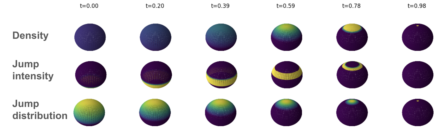
Figure 5: Illustration of jump model on manifolds. Left: Illustration of conditional probability $p_{t}(dx|z)$ on sphere with $z=(0,0,1)^{T}$ (North pole). Top: density $p_{t}(x|z)$. Middle: jump intensity $\lambda_{t}(x)=\int Q_{t}(dy;x)$. Bottom: Jump distribution $J_{t}(dy;x)=Q_{t}(dy;x)/\int Q_{t}(dy;x)$.

G.2 Probability paths and computing $\lambda_{t},J_{t}$

We consider the quaternion model for $SO(3)$, namely, each element of $SO(3)$ is represented by a unit vector $x\in{\mathcal{S}}^{3}\subset\mathbb{R}^{4}$, where

$${\mathcal{S}}^{3}=\big{\{}x\in\mathbb{R}^{4}\ \big{|}\ \|x\|=1\big{\}}$$ (46)

with $\|x\|=1$. We consider a probability path of Fisher-von-Mises distributions given by

$$p_{t}(x|x_{1})=C_{p}(\kappa_{t})\exp(\kappa_{t}x_{1}^{T}x)$$

for a scheduler $\kappa_{t}$ such that $\kappa_{0}=0$ and $\kappa_{1}>>0$ and normalization constant $C_{p}(\kappa_{t})$. We use a custom implementation of the Fisher-von-Mises distribution in a way that makes $p_{t}(x|x_{1})$ differentiable with respect to $t$. We then use automatic differentiation to compute $\partial_{t}p_{t}(x|x_{1})$. This allows us to compute $\lambda_{t}$ and $J_{t}$ (see previous section). To parameterize $\lambda_{t}$ on $SO(3)$, we simply consider a function on $SO(3)$. To parameterize $J_{t}$ on $SO(3)$ we place uniform bins over $SO(3)$ and make each bin represent a rotation. We note that the probability path that FrameFlow was trained on is not the probability path above. Rather, it is a probability path constructed via geodesic interpolation of a uniform to a delta function. Computing $\lambda_{t},J_{t}$ on this path was numerically unstable for us (because of sharp boundaries introduced by the uniform distribution). Therefore, we choose a Fisher-von-Mises path as above but selected the scheduler $\kappa_{t}$ to optimally approximate the geodesic path. This ensured numerical stability and an (approximately) faithful recovery of the probability path. The Fisher-von-Mises path is more numerically stable as its support is all of $SO(3)$ for all $0\leq t\leq 1$.

G.3 Sampling

The FrameFlow model predicts a data point $z$ given a state $x_{t}$ at time $0\leq t\leq 1$, i.e. it predicts the conditional expectation $\mathbb{E}_{z\sim p_{t}(dz|x)}[z]$. The marginal jump rate kernel is given by

$$Q_{t}(y;x_{t})=\mathbb{E}_{z\sim p_{t}(dz|x_{t})}[Q_{t}^{z}(y;x_{t})]$$

In order to repurpose the flow model, we make the simplifying assumption that

$$Q_{t}(y;x_{t})=\mathbb{E}_{z\sim p_{t}(dz|x_{t})}[Q_{t}^{z}(y;x_{t})]\approx Q_{t}^{\mathbb{E}_{z\sim p_{t}(dz|x_{t})}[z]}(y;x_{t})$$

Assuming that the distribution $p_{t}(dz|x)$ is unimodal, this corresponds to high temperature sampling of $z$. We do not employ any temperature to sample from $J_{t}$ or $\lambda_{t}$ but use plain Euler sampling as described in table 1.

G.4 Experiment details

We based our implementation off https://github.com/microsoft/protein-frame-flow/tree/legacy and downloaded pre-trained weights from the same repository. We use Euler-Maruyama integrator and 100 discretization steps for all sampling runs. We found increasing the number of bins to improve results and use 1024 in our experiments. For our metrics, we deviate slightly from (Yim et al., 2023a) by only reporting diversity and novelty and exclude designability. As noted in (Yim et al., 2024), designability can be artificially high if the generative model samples the same protein repeatedly. Nevertheles, using designability to filter bad samples is still important since protein generative models are prone to hallucination and producing proteins that would never be real. A detailed description of designability can be found in (Yim et al., 2023b). Our metrics already take designability into account by first filtering the sampled proteins to only be the designable proteins then clustering the protein structures to compute diversity and searching against protein datasets to measure novelty. Specifically, we first compute 10 samples for each length between 60 and 128 for a total of $n=690$ samples then compute each metric as follows:

1. Diversity (Div): Taking only the samples passing the designability filter, we use MaxCluster (Herbert & Sternberg, 2008) to compute the number of clusters $n_{c}$. We report $n_{n}/n$ which is the proportion of designable clusters to number of total samples. The higher this value, the more diverse the generated samples are after the designability filter. Diversity is important in protein design where it is ideal to test many diverse protein candidates in the hopes of having many shots to make a new drug or medicine for instance.

2. Novelty (Nov): Taking only the samples passing the designability filter, we use FoldSeek (Van Kempen et al., 2024) to compute the similarity of each sample to the Protein Data Bank (PDB) (Berman et al., 2000). The similarity score is given as a protein structure alignment score called the TM-score (Xu & Zhang, 2010) where a value of 0.5 or less means the two structures are likely to be distinct. The probability of the two structures being similar with the same biological function increases as the score goes to 1.0. Therefore, the dissimilarity is 1 - (TM-score). We report the average dissimilarity of the outputs of FoldSeek as the novelty since this describes how “novel” the designable samples are on average compared to the known protein structures.

Appendix H Extended discussion of related works

H.1 Flow matching

Flow matching and rectified flows (Lipman et al., 2022; Liu et al., 2022) are immediate instances of generator matching leveraging the flow-specific versions of the KFE given by the continuity equation (see table 1 and sec. A.4.1 for a derivation). We briefly describe here how one can map the propositions from this work to their work. Specifically, flow matching restricts itself to generators of the form $\mathcal{L}_{t}^{\theta}f(x)=\nabla f(x)^{T}u_{t}^{\theta}(x)$ for a vector field $u_{t}^{\theta}(x)$ parameterized by a neural network with parameters $\theta$. Given a conditional vector field $u_{t}(x|z)$ and a probability path $p_{t}(x|z)$, the corresponding marginal vector field in flow matching (see (Lipman et al., 2022, equation (8))) is given by

$$u_{t}(x)=\int u_{t}(x|z)\frac{p_{t}(x|z)p_{\text{data}}(z)}{p_{t}(x)}dz$$

and corresponds to the marginal generator (see proposition 1). The Bregman divergence used is the mean squared error (MSE) obtained by choosing $\phi(x)=\|x\|^{2}$ in eq. 10. The conditional flow matching loss (Lipman et al., 2022, Theorem 2 ) is a special case of proposition 2. Therefore, generator matching can be seen as a generalization of the principles of flow matching to the space of Markov process generators for arbitrary state spaces.

H.2 Denoising diffusion models

From the perspective of generator matching, denoising diffusion models (Song et al., 2020) are flow models with two conceptual differences to flow matching: (1) They allow for stochastic sampling via SDEs by adding a divergence-free Langevin component (see proposition 3) and (2) A probability path is defined via forward noising process and a time-reversal of that process serves a solution to the KFE. We explain both differences below.

Time-reversal to find solutions to the KFE.

First, let’s discuss the idea of time-reversal. In diffusion models, a probability path $p_{t}(dx|z)$ is thought of as a forward diffusion process that noises data. While this mathematically equivalent, the conceptual idea of time-reversal allows to find solutions to the KFE. We illustrate this here by deriving the time-reversal formula for denoising diffusion models here via the generator perspective. Specifically, let’s consider a Markov noising process $\bar{X}_{t}$ given by a variance-exploding SDE $d\bar{X}_{t}=\sigma_{t}d\bar{W}_{t}$ that goes from $t=1$ to $t=0$ backwards in time (note that in (Song et al., 2020) $t=0$ corresponds to data, while we keep the convention here that $t=1$ corresponds data). Then we know that the KFE holds in reverse time

$$\partial_{t}p_{t}f= -p_{t}\odot\bar{\mathcal{L}}_{t}f \blacktriangleright\text{ KFE in reverse time}$$

$$= -\int p_{t}(x)\frac{\sigma_{t}^{2}}{2}\Delta f(x)dx \blacktriangleright\text{ generator for diffusions, see table 1}$$

$$= -\int p_{t}(x)\frac{\sigma_{t}^{2}}{2}\nabla\cdot\nabla f(x)dx \blacktriangleright\text{ definition of Laplacian}$$

$$= \int\nabla p_{t}(x)^{T}\frac{\sigma_{t}^{2}}{2}\nabla f(x)dx \blacktriangleright\text{ partial integration}$$

$$= \int p_{t}(x)\underbrace{\nabla f(x)^{T}\left[\frac{\sigma^{2}_{t}}{2}\nabla\log p_{t}(x)\right]}_{=:\mathcal{L}_{t}f(x)}dx \blacktriangleright\text{ derivative of log}$$

$$= p_{t}\odot\mathcal{L}_{t}f$$

Therefore, $\mathcal{L}_{t}f=f^{T}\frac{\sigma_{t}^{2}}{2}\nabla\log p_{t}$ corresponds to a generator of a flow that solves the KFE in forward time (i.e. generating data). This corresponds to what is commonly called the probability flow ODE (Song et al., 2020) with vector field $\frac{\sigma_{t}^{2}}{2}\nabla\log p_{t}$. The conditional generator matching loss with a mean squared error then leads to the denoising score matching loss (Vincent, 2011)

$$\mathbb{E}_{z\sim p_{\text{data}},t\sim\text{Unif},x\sim p_{t}(\cdot|z)}[\|\nabla\log p_{t}(x|z)-s_{\theta}(x,t)\|^{2}]$$

for a neural network $s_{\theta}:\mathbb{R}^{d}\times[0,1]\to\mathbb{R}^{d}$ approximating the score vector field. We remark that mathematically there is also a stronger notion of time-reversal that also requires the joint distribution (across time points) to the be same - as opposed to just the marginals.

Stochastic sampling by adding a divergence component.

Second, let’s discuss stochastic sampling. For a general probability path $p_{t}$ with density $p_{t}(x)$, a general divergence-free component is given via the Langevin generator corresponding to an SDE with drift $\sigma_{t}^{2}\nabla\log p_{t}(x)$ and diffusion coefficient $\sqrt{2\sigma_{t}}$

$$\mathcal{L}_{t}^{\text{Langevin}}f(x)=\sigma_{t}^{2}\nabla f(x)^{T}\nabla\log p_{t}(x)+\sigma_{t}^{2}\Delta f(x),$$ (47)

This fact is widely applied in statistical physics and Markov chain Monte Carlo methods in the form of Langevin dynamics (Roberts & Tweedie, 1996). To see that this is divergence-free (in the sense as defined in proposition 3), we can simply use partial integration

$$p_{t}\odot\mathcal{L}_{t}^{\text{Langevin}}f= \int p_{t}(x)\sigma_{t}^{2}\nabla f(x)^{T}\nabla\log p_{t}(x)dx+\int p_{t}(x)\sigma_{t}^{2}\Delta f(x)dx \blacktriangleright\text{ by definition}$$

$$= \int\sigma_{t}^{2}\nabla f(x)^{T}\nabla p_{t}(x)dx+\int p_{t}(x)\sigma_{t}^{2}\Delta f(x)dx \blacktriangleright\text{ derivative of log}$$

$$= -\int\sigma_{t}^{2}\Delta f(x)p_{t}(x)dx+\int p_{t}(x)\sigma_{t}^{2}\Delta f(x)]dx \blacktriangleright\text{ partial integration}$$

$$= 0$$

In (Song et al., 2020), they fix a specific weighting and run several iterations of a Langevin sampling iteration at every time step, there called a predictor-corrector scheme (see (Song et al., 2020, Algorithm 1-3)). However, by proposition 3 any positive weighting of the above Langevin component leads to a valid sampling procedure. This observation was already made by Karras et al. (2022, section 4) where the optimal weighting of the divergence-free Langevin component is studied experimentally in more detail.

Finally, we note that many denoising diffusion models use formulations in discrete time (Sohl-Dickstein et al., 2015; Ho et al., 2020). While these formulations do not incur a time discretization error during sampling, they incur an error in the loss formulation. The reason for that is that a similar proposition as in proposition 2 does not hold for discrete time steps (i.e. the linearization only holds for the generator and not the transition kernel). Therefore, a formulation with discrete time steps can only us an approximate loss via an ELBO lower bound using parameterized family of distributions such as a Gaussian (Sohl-Dickstein et al., 2015).

H.3 Stochastic Interpolants

Stochastic interpolants (Albergo & Vanden-Eijnden, 2022; Albergo et al., 2023) is a framework for generative modelling that shares many similarities with diffusion models and flow matching. We explain conceptual differences by placing its findings within the generator matching framework.

General flow solution based on interpolant.

A difference in the perspective of stochastic interpolants is that they take a sample-based perspective, i.e. they specific an initial distribution $x_{0}\sim p_{0}$ and a probability path $x_{t}\sim p_{t}(dx)$ is constructed implicitly via a simulator function $I$ (see (Albergo et al., 2023, definition 2.1))

$$x_{t}:=\Phi(t,x_{0},z,\epsilon):=I(t,x_{0},z)+\gamma(t)\epsilon$$ (48)

where $\epsilon\sim\mathcal{N}(0,I_{d})$ and we impose the condition that $I(0,x_{0},z)=x_{0}$, $I(1,x_{0},z)=z$ and $\gamma(0)=0,\gamma(1)=0$. A general flow-based solution can be derived by using the KFE (see (Albergo et al., 2023, theorem 2.6)):

$$\frac{\partial}{\partial t}p_{t}\odot f=\partial_{t}\mathbb{E}[f(\Phi(t,x_{0},z,\epsilon))]= \mathbb{E}[\nabla f(\Phi(t,x_{0},z,\epsilon))^{T}\partial_{t}\Phi(t,x_{0},z,\epsilon)]$$

$$= \mathbb{E}_{x_{t}\sim p_{t}}[\underbrace{\nabla f(x_{t})^{T}\mathbb{E}[\partial_{t}\Phi(t,x_{0},z,\epsilon)|x_{t}]}_{=:\mathcal{L}_{t}f(x_{t})}]$$

$$= \mathbb{E}_{x_{t}\sim p_{t}}[\mathcal{L}_{t}f(x_{t})]$$

The operator $\mathcal{L}_{t}f$ is a generator of a flow with vector field given by the conditional expectation of the velocity $u(x_{t},t)=\mathbb{E}[\partial_{t}\Phi(t,x_{0},z,\epsilon)|x_{t}]$. Hence, we see that the above vector field generates the probability path $p_{t}$. This can be trained in the same way with a mean-squared error as for denoising diffusion models and flow matching.

Stochastic sampling.

Another difference of stochastic interpolants is a generalization of the stochastic sampling procedure for denoising diffusion models (see sec. H.2). One advantage of denoising diffusion models is that one gets - informally - "2 advantages for 1": Specifically, both for learning a flow-based solution to the KFE and for stochastic sampling, we only need to learn the function $\nabla\log p_{t}$ commonly called the score function (see sec. H.2). This works because the process is constructed as a diffusion process. However, in the general case, one can still learn the score $\nabla\log p_{t}$ separately from the flow and then add a divergence-free Langevin component during sampling (see eq. 47). As pointed out in (Albergo et al., 2023, theorem 2.8), the special shape of the stochastic interpolant (see eq. 48) allows to derive a simple denoising score matching loss. In (Albergo et al., 2023, theorem 2.23), it is further shown that adding stochastic sampling leads to the ability to control the KL-divergence between the target distribution and the distribution generated by the model. This highlights an advantage of adding a noise (SDE) term because bounding the KL-divergence is in general not possible with a pure flow model (although bounds in Wasserstein distance exist for flow models, see (Benton et al., 2023)).

H.4 Language Models via Continuous-Time Markov Chains ("Discrete Diffusion")

For discrete state spaces $S$, the generator of a Markov process $X_{t}\in S$ is given by a rate transition matrix $Q_{t}\in\mathbb{R}^{S\times S}$ (see sec. A.4.4 for derivations). Therefore, if we restrict ourselves to generators on discrete state spaces, we recover the framework developed by (Campbell et al., 2022) as an instance of generator matching. Proposition 1 in Campbell et al. (2022) corresponds to proposition 1 showing that the marginal generator/rate matrix corresponds a conditional generator weighted by the posterior. Proposition 2 in Campbell et al. (2022) shows that a continuous-time ELBO can be derived via a Bregman divergence. We derive a similar, slightly simpler, Bregman divergence loss in sec. D.2 that also corresponds to an ELBO lower bound. Further, they use a predictor-corrector scheme (see Campbell et al. (2022, Proposition 4)) as outlined here for the general case in proposition 3. In the discrete setting, this leads to significant improvements (Gat et al., 2024).

In many applications such as language modelling, the state space decomposes into dimensions, i.e. is given via $S=\{1,\dots,N\}^{d}=:[N]^{d}$ where $N$ is the vocabulary size. This state space is usually too large that one cannot store a full rate transition matrix $Q_{t}$ (and not even a single row of it) in a computer. However, using a factorized probability path, we can use proposition 4 to see that we can learn a rates $Q_{t}$ that update each dimension independently (i.e. it has a block structure). This reduces the dimension significantly. This was shown for discrete spaces also in Campbell et al. (2022, Proposition 3) and has since then the de facto standard for discrete diffusion models (Lou et al., 2024a; Gat et al., 2024). Instead of parameterizing the generator directly, proposition 4 also shows that one can also only learns the marginals $p_{t}(z_{i}|x)$ for each $z=(z_{1},\dots,z_{n})\in[N]^{d}$ independently. One can then train the marginals of the posterior $p_{t}(z_{i}|x)$ via the cross-entropy loss (Gat et al., 2024; Campbell et al., 2024).

Campbell et al. (2022) adapt the idea of time-reversal from diffusion models to find solutions of the KFE for a given probability path. Specifically, the time-reversal $Q_{t}$ of a process with rate matrix $\bar{Q}_{t}$ running in backwards-time is given via

$$Q_{t}(x;y)=\bar{Q}_{t}(y;x)\frac{p_{t}(x)}{p_{t}(y)}$$

In more recent works (Lou et al., 2024a), it has been shown that parmeterizing the generator by the ratio $p(y)/p(x)$ that is needed to time-reverse the process - called the "discrete score" - leads to improved results. As this is a linear parameterization of the generator, they can use the same Bregman divergence as we derive in sec. D.2 to train the discrete score.

H.5 Geometric data and Manifolds

We next describe how generator matching generalizes models on Riemannian manifolds. In the following, let $S=\mathcal{M}$ be a smooth Riemannian manifold with metric $g$. For $x\in\mathcal{M}$, let $T_{x}\mathcal{M}$ be the tangent space of $x$ and let $T\mathcal{M}=\bigsqcup_{x\in\mathcal{M}}T_{x}\mathcal{M}$ be the tangent bundle.

Riemannian Flow Matching (Chen & Lipman, 2024).

First, we consider flows on $\mathcal{M}$ showing how we can recover Riemannian Flow Matching (Chen & Lipman, 2024). A flow on $\mathcal{M}$ is defined via a vector field $u:\mathcal{M}\times[0,1]\to T\mathcal{M}$ such that $u_{t}(x)\in T_{x}\mathcal{M}$ for all $x\in\mathcal{M}$. As every tangent space is a vector space, the space of vector fields is a vector space again. Every vector fields defines a flow $\phi_{t|s}$ that fulfils

$$\phi_{t|t}(x)= x\text{ for all }0\leq t\leq 1$$

$$\frac{d}{dt}\phi_{t|s}(x)= u_{t}(\phi_{t|s}(x))\text{ for all }0\leq s\leq t\leq 1$$

Next, we derive the generator. Let $f:\mathcal{M}\to\mathbb{R}$ be a smooth function. Then the generator is given via

$$\mathcal{L}_{t}f(x)=\lim\limits_{h\to 0}\frac{f(\phi_{t+h|t}(x))-f(x)}{h}=\left\langle\nabla f(x),u_{t}(x)\right\rangle_{g}$$

where $\left\langle\cdot,\cdot\right\rangle_{g}$ describes the dot product defining the Riemannian metric $g$ and $\nabla f$ describes the gradient of $f$ with respect to $g$. This coincides with the Lie derivative of a function (Jost & Jost, 2008), a fundamental concept in differential geometry. Therefore, we see that $u_{t}(x)$ is a linear parameterization of the generator. We can then use an arbitrary Bregman divergence on $T_{x}\mathcal{M}$, e.g. the mean-squared error. The CGM loss then recovers the Riemannian Conditional Flow Matching loss (see (Chen & Lipman, 2024, equation (8))). This shows that Riemannian Flow Matching is a specific instance of generator matching with Markov processes on manifolds restricted to flows.

Diffusion models on manifolds (De Bortoli et al., 2022; Huang et al., 2022).

Riemannian score-based generative modeling can equally be seen as an instance of GM. Similar to Euclidean diffusion models, a probability path is constructed via a forward noising process and a solution to the KFE is found via a time-reversal of the process (see sec. H.2 as an example on Euclidean space). Specifically, a forward-time SDE that generates data is obtained via time-reversal (see (De Bortoli et al., 2022, theorem 3.1.)) and has the shape

$$dY_{t}= [-b(Y_{t})+\nabla\log p_{t}(Y_{t})]dt+dB_{t}^{\mathcal{M}}$$

where $b:\mathcal{M}\to T\mathcal{M}$ describes a drift, $\nabla\log p_{t}:\mathcal{M}\to T\mathcal{M}$ describe the score vector field and $\mathcal{B}_{t}^{\mathcal{M}}$ describes a Brownian motion on $\mathcal{M}$. The generator of the above SDE is given via

$$\mathcal{L}_{t}f(x)=-\left\langle b(x),\nabla f(x)\right\rangle_{g}+\left\langle\nabla f(x),\nabla\log p_{t}(x)\right\rangle_{g}+\frac{1}{2}\Delta_{\mathcal{M}}f(x)$$

where $\Delta_{g}f$ describes the Laplace-Beltrami operator on manifolds (Elworthy, 1998). Note that $b$ is fixed as a hyperparameter. Therefore, like in the Euclidean case, a linear parameterization of the generator is again given via a score network $s_{\theta}:\mathcal{M}\times[0,1]\to T\mathcal{M}$. Choosing the mean squared error as a Bregman divergence, one recovers Riemannian denoising score matching (see (De Bortoli et al., 2022, section 3.2)). However, the fact that the noising process is not analytically tractable does not give us an analytically tractable formula for $p_{t}(x|z)$, i.e. in GM language the conditional solution to the KFE is not known analytically. Therefore, this approach requires iterative simulation of a noising process during training even for geometries with analytic geodesic formulas and requires approximations of score functions as a training target (see (De Bortoli et al., 2022, table 2)).

H.6 Multimodal spaces

Markovian multimodal generative models have been previously described for specific spaces and model classes (Anand & Achim, 2022; Campbell et al., 2024). As an example, we illustrate here how the work by Campbell et al. (2024) for multimodal protein generation fits into the GM framework.

Campbell et al. (2024) first construct a generative model on discrete spaces representing amino acids of a protein using the recipe outlined in (Campbell et al., 2022) (see sec. H.4 for explanations how this fits into GM framework). Further, they use a Euclidean flow model (Lipman et al., 2022) for the translation components of the protein and a Riemannian Flow model (Yim et al., 2024) is used for frames represented via elements on $SO(3)$. Using a factorized probability, one can use the recipe outlined in proposition 4 to build a multimodal generative model. This corresponds to Proposition 4.1. and Proposition 4.2. in (Campbell et al., 2024). As outlined in proposition 4, loss functions for individual modalities can be summed up, as done in (Campbell et al., 2024, equation (16)). Therefore, the work by Campbell et al. (2024) is a direct example of the power of the recipe outlined in proposition 4 to build a Markovian generative model.

References

• Albergo & Vanden-Eijnden (2022) Michael S Albergo and Eric Vanden-Eijnden. Building normalizing flows with stochastic interpolants. arXiv preprint arXiv:2209.15571, 2022.
• Albergo et al. (2023) Michael S Albergo, Nicholas M Boffi, and Eric Vanden-Eijnden. Stochastic interpolants: A unifying framework for flows and diffusions. arXiv preprint arXiv:2303.08797, 2023.
• Ambrosio (2004) Luigi Ambrosio. Transport equation and cauchy problem forbvvector fields. Inventiones mathematicae, 158(2), 2004.
• Anand & Achim (2022) Namrata Anand and Tudor Achim. Protein structure and sequence generation with equivariant denoising diffusion probabilistic models. arXiv preprint arXiv:2205.15019, 2022.
• Benton et al. (2023) Joe Benton, George Deligiannidis, and Arnaud Doucet. Error bounds for flow matching methods. arXiv preprint arXiv:2305.16860, 2023.
• Benton et al. (2024) Joe Benton, Yuyang Shi, Valentin De Bortoli, George Deligiannidis, and Arnaud Doucet. From denoising diffusions to denoising markov models. Journal of the Royal Statistical Society Series B: Statistical Methodology, 86(2):286–301, 2024.
• Berman et al. (2000) Helen M Berman, John Westbrook, Zukang Feng, Gary Gilliland, Talapady N Bhat, Helge Weissig, Ilya N Shindyalov, and Philip E Bourne. The protein data bank. Nucleic acids research, 28(1):235–242, 2000.
• Bogachev et al. (2022) Vladimir I Bogachev, Nicolai V Krylov, Michael Röckner, and Stanislav V Shaposhnikov. Fokker–Planck–Kolmogorov Equations, volume 207. American Mathematical Society, 2022.
• Campbell et al. (2022) Andrew Campbell, Joe Benton, Valentin De Bortoli, Thomas Rainforth, George Deligiannidis, and Arnaud Doucet. A continuous time framework for discrete denoising models. Advances in Neural Information Processing Systems, 35:28266–28279, 2022.
• Campbell et al. (2024) Andrew Campbell, Jason Yim, Regina Barzilay, Tom Rainforth, and Tommi Jaakkola. Generative flows on discrete state-spaces: Enabling multimodal flows with applications to protein co-design. arXiv preprint arXiv:2402.04997, 2024.
• Chen & Lipman (2024) Ricky T. Q. Chen and Yaron Lipman. Flow matching on general geometries. In The Twelfth International Conference on Learning Representations, 2024.
• Chen et al. (2018) Ricky T. Q. Chen, Yulia Rubanova, Jesse Bettencourt, and David K Duvenaud. Neural ordinary differential equations. Advances in neural information processing systems, 31, 2018.
• Courrege (1965) Philippe Courrege. Sur la forme intégro-différentielle des opérateurs de $c^{\infty}_{k}$ dans $c$ satisfaisant au principe du maximum. Séminaire Brelot-Choquet-Deny. Théorie du Potentiel, 10(1):1–38, 1965.
• Davis (1984) Mark HA Davis. Piecewise-deterministic markov processes: A general class of non-diffusion stochastic models. Journal of the Royal Statistical Society: Series B (Methodological), 46(3):353–376, 1984.
• De Bortoli et al. (2022) Valentin De Bortoli, Emile Mathieu, Michael Hutchinson, James Thornton, Yee Whye Teh, and Arnaud Doucet. Riemannian score-based generative modelling. Advances in Neural Information Processing Systems, 35:2406–2422, 2022.
• DiPerna & Lions (1989) Ronald J DiPerna and Pierre-Louis Lions. Ordinary differential equations, transport theory and sobolev spaces. Inventiones mathematicae, 98(3):511–547, 1989.
• Elworthy (1998) Kenneth David Elworthy. Stochastic differential equations on manifolds. Springer, 1998.
• Ethier & Kurtz (2009) Stewart N Ethier and Thomas G Kurtz. Markov processes: characterization and convergence. John Wiley & Sons, 2009.
• Feller (1955) William Feller. On second order differential operators. Annals of Mathematics, 61(1):90–105, 1955.
• Figalli (2008) Alessio Figalli. Existence and uniqueness of martingale solutions for sdes with rough or degenerate coefficients. Journal of Functional Analysis, 254(1):109–153, 2008.
• Gat et al. (2024) Itai Gat, Tal Remez, Neta Shaul, Felix Kreuk, Ricky T. Q. Chen, Gabriel Synnaeve, Yossi Adi, and Yaron Lipman. Discrete flow matching. arXiv preprint arXiv:2407.15595, 2024.
• Goodfellow et al. (2014) Ian Goodfellow, Jean Pouget-Abadie, Mehdi Mirza, Bing Xu, David Warde-Farley, Sherjil Ozair, Aaron Courville, and Yoshua Bengio. Generative adversarial nets. Advances in neural information processing systems, 27, 2014.
• Herbert & Sternberg (2008) Alex Herbert and MJE Sternberg. MaxCluster: a tool for protein structure comparison and clustering. 2008.
• Ho et al. (2020) Jonathan Ho, Ajay Jain, and Pieter Abbeel. Denoising diffusion probabilistic models. Advances in neural information processing systems, 33:6840–6851, 2020.
• Huang et al. (2022) Chin-Wei Huang, Milad Aghajohari, Joey Bose, Prakash Panangaden, and Aaron C Courville. Riemannian diffusion models. Advances in Neural Information Processing Systems, 35:2750–2761, 2022.
• Jost & Jost (2008) Jürgen Jost and Jeurgen Jost. Riemannian geometry and geometric analysis, volume 42005. Springer, 2008.
• Karras et al. (2022) Tero Karras, Miika Aittala, Timo Aila, and Samuli Laine. Elucidating the design space of diffusion-based generative models. Advances in Neural Information Processing Systems, 35:26565–26577, 2022.
• Kingma (2013) Diederik P Kingma. Auto-encoding variational bayes. arXiv preprint arXiv:1312.6114, 2013.
• Kurtz (2011) Thomas G Kurtz. Equivalence of stochastic equations and martingale problems. Stochastic analysis 2010, pp.  113–130, 2011.
• Lipman et al. (2022) Yaron Lipman, Ricky T. Q. Chen, Heli Ben-Hamu, Maximilian Nickel, and Matt Le. Flow matching for generative modeling. arXiv preprint arXiv:2210.02747, 2022.
• Liu et al. (2022) Xingchao Liu, Chengyue Gong, and Qiang Liu. Flow straight and fast: Learning to generate and transfer data with rectified flow. arXiv preprint arXiv:2209.03003, 2022.
• Lou et al. (2024a) Aaron Lou, Chenlin Meng, and Stefano Ermon. Discrete diffusion modeling by estimating the ratios of the data distribution. stat, 1050:21, 2024a.
• Lou et al. (2024b) Aaron Lou, Chenlin Meng, and Stefano Ermon. Discrete diffusion modeling by estimating the ratios of the data distribution. In Forty-first International Conference on Machine Learning, 2024b.
• Oksendal (2013) Bernt Oksendal. Stochastic differential equations: an introduction with applications. Springer Science & Business Media, 2013.
• Opper & Sanguinetti (2007) Manfred Opper and Guido Sanguinetti. Variational inference for markov jump processes. Advances in neural information processing systems, 20, 2007.
• Pazy (2012) Amnon Pazy. Semigroups of linear operators and applications to partial differential equations, volume 44. Springer Science & Business Media, 2012.
• Pooladian et al. (2023) Aram-Alexandre Pooladian, Heli Ben-Hamu, Carles Domingo-Enrich, Brandon Amos, Yaron Lipman, and Ricky T. Q. Chen. Multisample flow matching: Straightening flows with minibatch couplings. International Conference on Machine Learning, 2023.
• Roberts & Tweedie (1996) Gareth O Roberts and Richard L Tweedie. Exponential convergence of langevin distributions and their discrete approximations. Bernoulli 2(4): 341-363 (December 1996), 1996.
• Rogers & Williams (2000) Leonard CG Rogers and David Williams. Diffusions, markov processes, and martingales: Volume 1, foundations. Cambridge university press, 2000.
• Rüschendorf et al. (2016) Ludger Rüschendorf, Alexander Schnurr, and Viktor Wolf. Comparison of time-inhomogeneous markov processes. Advances in Applied Probability, 48(4):1015–1044, 2016.
• Sohl-Dickstein et al. (2015) Jascha Sohl-Dickstein, Eric Weiss, Niru Maheswaranathan, and Surya Ganguli. Deep unsupervised learning using nonequilibrium thermodynamics. In International conference on machine learning, pp.  2256–2265. PMLR, 2015.
• Song et al. (2020) Yang Song, Jascha Sohl-Dickstein, Diederik P Kingma, Abhishek Kumar, Stefano Ermon, and Ben Poole. Score-based generative modeling through stochastic differential equations. arXiv preprint arXiv:2011.13456, 2020.
• Tong et al. (2023) Alexander Tong, Nikolay Malkin, Guillaume Huguet, Yanlei Zhang, Jarrid Rector-Brooks, Kilian Fatras, Guy Wolf, and Yoshua Bengio. Improving and generalizing flow-based generative models with minibatch optimal transport. arXiv preprint arXiv:2302.00482, 2023.
• Van Kempen et al. (2024) Michel Van Kempen, Stephanie S Kim, Charlotte Tumescheit, Milot Mirdita, Jeongjae Lee, Cameron LM Gilchrist, Johannes Söding, and Martin Steinegger. Fast and accurate protein structure search with foldseek. Nature biotechnology, 42(2):243–246, 2024.
• Villani et al. (2009) Cédric Villani et al. Optimal transport: old and new, volume 338. Springer, 2009.
• Vincent (2011) Pascal Vincent. A connection between score matching and denoising autoencoders. Neural computation, 23(7):1661–1674, 2011.
• von Waldenfels (1965) Wilhelm von Waldenfels. Fast positive operatoren. Zeitschrift für Wahrscheinlichkeitstheorie und Verwandte Gebiete, 4:159–174, 1965.
• Xu & Zhang (2010) Jinrui Xu and Yang Zhang. How significant is a protein structure similarity with tm-score= 0.5? Bioinformatics, 26(7):889–895, 2010.
• Yim et al. (2023a) Jason Yim, Andrew Campbell, Andrew YK Foong, Michael Gastegger, José Jiménez-Luna, Sarah Lewis, Victor Garcia Satorras, Bastiaan S Veeling, Regina Barzilay, Tommi Jaakkola, et al. Fast protein backbone generation with se (3) flow matching. arXiv preprint arXiv:2310.05297, 2023a.
• Yim et al. (2023b) Jason Yim, Brian L Trippe, Valentin De Bortoli, Emile Mathieu, Arnaud Doucet, Regina Barzilay, and Tommi Jaakkola. Se (3) diffusion model with application to protein backbone generation. arXiv preprint arXiv:2302.02277, 2023b.
• Yim et al. (2024) Jason Yim, Andrew Campbell, Emile Mathieu, Andrew YK Foong, Michael Gastegger, José Jiménez-Luna, Sarah Lewis, Victor Garcia Satorras, Bastiaan S Veeling, Frank Noé, et al. Improved motif-scaffolding with se (3) flow matching. arXiv preprint arXiv:2401.04082, 2024.
Refer to caption