SIGMA: Single Interpolated Generative Model for Anomalies

Abstract

A key step in any resonant anomaly detection search is accurate modeling of the background distribution in each signal region. Data-driven methods like CATHODE accomplish this by training separate generative models on the complement of each signal region, and interpolating them into their corresponding signal regions. Having to re-train the generative model on essentially the entire dataset for each signal region is a major computational cost in a typical sliding window search with many signal regions. Here, we present SIGMA, a new, fully data-driven, computationally-efficient method for estimating background distributions. The idea is to train a single generative model on all of the data and interpolate its parameters in sideband regions in order to obtain a model for the background in the signal region. The SIGMA method significantly reduces the computational cost compared to previous approaches, while retaining a similar high quality of background modeling and sensitivity to anomalous signals.

I Introduction

There has been a rapid growth in new methods for resonant anomaly detection in recent years [1, 2, 3, 4, 5, 6, 7, 8, 9, 10, 11, 12, 13, 14, 15, 16, 17, 18, 19, 20, 21, 22, 23, 24, 25, 26, 27, 28, 29, 30, 31]. These methods are starting to move from proof-of-concept to actual analyses applied to ATLAS [32] and CMS data [33] in the model-agnostic search for new physics. They have also been successfully applied to astronomical data from the Gaia Space Telescope in the search for stellar streams [34, 35, 36, 37].

In resonant anomaly detection, one uses additional features $x$ to enhance the sensitivity of a “bump hunt” in a primary feature $m$ where the signal is assumed to be localized. The overall goal is to accurately estimate the Neyman-Pearson classifier

$$R_{\rm optimal}(x)={p_{\rm data}(x)\over p_{\rm background}(x)}$$ (1)

in a signal region (SR), which is defined as a window in $m$. By cutting on this “optimal anomaly score”, one can preferentially select signal over background events in a model-agnostic way, i.e. without having to specify the signal model in advance.

In many approaches, a key step is to learn a fully data-driven estimate for $p_{\rm background}(x)$ by interpolating from from neighboring control regions (CR) in $m$. In methods like ANODE [3] and CATHODE [7], one trains a generative model and/or density estimator (e.g. a conditional normalizing flow) on the complement of the signal region, which for a narrow signal region is almost the entire dataset. For each signal region this must be performed separately, and this leads to extremely expensive trainings for a full sliding-window search.

There have been efforts to mitigate this computational cost. In CURTAINSF4F [26], one can train a single flow on the entire dataset, not masking out the SR, and another conditional flow on short control regions to learn the transformation between them. This can then be used to interpolate into the signal region and saves significantly on computational cost since the all-data flow need only be learned once, and the short control region flow is usually learned on significantly less data.

Recently in RAD-OT [30], the idea was to dispense with the flow altogether and just use OT to transport sidebands to sidebands, thereby interpolating into the SR. This was shown to be computationally very inexpensive but at the cost of sacrificing some quality in the interpolation.

In this paper, we present a Single Interpolated Generative Model for Anomalies (SIGMA), a new approach for computationally efficient resonant anomaly detection, which is much simpler than CURTAINSF4F and maintains the high quality of the more expensive methods like CATHODE. Our idea is to train a single flow on all the data, as in CURTAINSF4F, and simply interpolate the parameters of the flow in the resonant feature. We find the simplest implementation of this is using flow-matching, where the vector field itself can be easily interpolated into the signal region. We will demonstrate that SIGMA produces high quality background samples while saving significantly on training cost – even more than CURTAINSF4F since even the short sideband flows can be dispensed with.

This paper is organized as follows: in Section II.1 we describe the dataset used to demonstrate our method. The architecture of the generative model used for our background template is described in  II.2.2. In II.3.1 we describe the slower interpolation method from [3, 7] using flow-matching. The new interpolation method SIGMA is described in Section II.3.2. The model hyperparameters and the training are described in Section II.4. In Section III, we show the results for anomaly detection, and the background template obtained from different methods. Finally in Section IV we present our conclusions and further discussion. In Appendix A, we discuss the importance of using frequency embedding for SIGMA. In Appendix B we analyze the background templates using the classifier test, developed in [38].

II Setup

II.1 Dataset

We use the LHCO R&D Dataset [39, 40] for this study with dataset and train-val-test splits similar to [7, 3]. The Standard Model(SM) background consists of QCD dijet events, and $W^{\prime}\rightarrow X(\rightarrow qq)Y(\rightarrow qq)$ events with $m_{W^{\prime}}=3.5\,\text{TeV}$, $m_{X}=500\,\text{GeV}$ and $m_{Y}=100\,\text{GeV}$ form the signal. These are simulated using Pythia 8 [41, 42] and Delphes 3.4.1 [43, 44, 45]. The reconstructed particles are clustered into jets using the anti-$k_{T}$ algorithm [46, 47] with $R=1$ using Fastjet [48]. Events that satisfy the $p_{T}>1.2\,\text{TeV}$ jet trigger are kept.

The training features we use are:

$$m=m_{JJ},\quad x=[m_{J_{1}},\Delta m_{J},{\tau_{21}}^{J_{1}},{\tau_{21}}^{J_{2}},\Delta R],$$ (2)

where invariant masses of the subjets satisfy $m_{J_{1}}<m_{J_{2}}$, and $\Delta m_{J}=m_{J_{2}}-m_{J_{1}}$. We chose dijet invariant mass $m_{JJ}$ as the resonant variable $m$, with the signal region (SR) defined as $m\in[3.3,3.7]$ and $m\notin[3.3,3.7]$ form the control regions (CR). The n-subjettiness ratios are $\tau_{ij}=\tau_{i}/\tau_{j}$ [49, 50]. $\Delta R$ is the angular separation of the leading two jets in $\eta-\phi$ space. Including it does not enhance the performance for anomaly detection, compared to just baseline features. But it is a feature that is strongly correlated with the resonant feature, $m_{JJ}$, and hence including it provides a stringent test for any interpolation method [51].

We use all $1$-million SM background events from the original R&D dataset and inject different amounts of signal (3000 or lower) from the first 70k signal events of the R&D dataset. This is meant to represent actual un-labeled data from the experiment. For reference, the signal-injection of $N_{\rm sig}=1000$ corresponds to $\approx 2.2\sigma$ significance for the inclusive bump hunt in $m_{JJ}$.

Figure 1: ResNet architecture

We split this dataset into training and validation sets, with 85-15 split for training all generative models. For IAD, following [7], we classify between data in SR and an additional 272k QCD dijet events in the SR [52] (which represents true background). For CATHODE, we classify between data in SR, and 360k events sampled from the 10 best instances of the trained generative model. We use the remaining 30k signal events from the original R&D dataset, along with the additional 340k QCD dijet events in the SR from [52] for evaluating SIC curves.

For each $N_{\rm sig}$, we produce ten different datasets by injecting different randomly selected signal events from the R&D dataset. This is used to obtain the error bars on the performance curves in the figures.

II.2 Flow-matching and Network Architecture

We use Conditional Flow Matching [53, 54, 55] to model the background template as a proof of concept, but our idea could be extended to be used with Diffusion models [56] as well. Besides providing a better quality background template than ordinary normalizing flows, we found that flow matching also trains faster – in approximately 30 mins, as compared to a normalizing flow which trains in $\sim$ 2.8 hours. In this section, we give a brief description of conditional flow-matching and then describe the neural network architecture used to model the flow.

II.2.1 Conditional Flow Matching

Conditional Flow Matching (CFM) [53, 57, 58, 59, 60] is an efficient way to train Continuous Normalizing Flows (CNFs) [61]. In CNFs, one aims to learn the vector field $u_{t}(x_{t}):[0,1]\times\mathbb{R}^{d}\to\mathbb{R}^{d}$ which implements a continuous transformation of data $x_{t}$ via:

$$\frac{dx_{t}}{dt}=u_{t}(x_{t}),$$ (3)

At $t=0$, $x_{0}$ follows the data distribution $p_{\text{data}}(x_{0})$, and at $t=1$, $x_{1}$ follows a known distribution $p_{\text{base}}(x_{1})$. Here we take $p_{\text{base}}(x)$ to be the unit normal distribution $\mathcal{N}(x|0,1)^{d}$. In between, $x_{t}$ is sampled from a density $p_{t}(x_{t})$ which is generated by the vector field; the trajectory of these densities is referred to as the probability density path.

Training CNFs with maximum likelihood is extremely computationally expensive, because each evaluation of the likelihood requires solving an ODE. The breakthrough insight of Conditional Flow Matching is that one can instead regress the desired vector field $u_{t}(x_{t})$ with an MSE-type loss, by matching it to a conditional vector field $u_{t}(x_{t}|x_{0})$. This generates a conditional probability path $p_{t}(x|x_{0})$ where at $t=0$, we have $p_{0}(x|x_{0})=\mathcal{N}(x|x_{0},\sigma^{2}I)$ where $\sigma^{2}$ is very small, and at $t=1$, we have $p_{1}(x|x_{0})=\mathcal{N}(x|0,1)^{d}$. Marginalizing this path over the data distribution $p_{\text{data}}(x_{0})$ gives us the unconditional probability $p_{t}(x)$:

$$p_{t}(x)=\int dx_{0}\,p_{t}(x|x_{0})p_{\text{data}}(x_{0}).$$ (4)

In CFM, this conditional vector field is regressed with a neural network $v_{\theta}(x_{t}|t)$ by minimizing the CFM loss

$$\mathcal{L}(\theta)=\left\|v_{\theta}(x_{t}|t)-u_{t}\left(x_{t}|x_{0}\right)\right\|^{2},$$ (5)

In [53], it was shown that the CFM objective, when averaged over $t\sim\mathcal{U}[0,1]$, $x_{0}\sim p_{\text{data}}(x_{0})$ and $x_{t}\sim p_{t}(x|x_{0})$, is minimized by $v_{\theta}(x|t)=u_{t}(x)$. In addition to $t$, our models also have an additional conditional feature: $m$, the resonant feature, which allows us to model the vector field $u_{t}(x|m)$ corresponding to $p(x|m)$. After integrating equation (3) to obtain $x_{t}$, $p(x_{0}|m)$ can be obtained using:

$$\log p(x_{0}|m)=\log(x_{1})-\int_{1}^{0}dt\ \nabla_{x_{t}}.u_{t}(x_{t}|m).$$ (6)

II.2.2 Network Architecture

Similar to [24], we use a ResNet-style [62] architecture to model the vector field $u_{t}(x|m)$, since it is more expressive than an MLP. Rather than pass $m$ and $t$ directly to the ResNet, it is beneficial to first map them to an embedding space. For $t$, we use a frequency embedding $\beta:[0,1]\rightarrow\mathbb{R}^{2(L^{\prime}+1)}$ , similar to those used in diffusion models [56]:

$$\begin{split}\beta(t)=&\left(\sin(\pi t),\cos(\pi t),\dots,\right.\\ &\left.\sin((L^{\prime}+1)\pi t),\cos((L^{\prime}+1)\pi t)\right).\end{split}$$ (7)

The resonant feature $m$ is first rescaled to $[-1,1]$, and then mapped to an embedding space $\alpha:[-1,1]\rightarrow\mathbb{R}^{2L}$. Depending on the interpolation method, we find different embeddings are preferable, see Sec. II.3 for more details. The $t$ and $m$ embeddings are concatenated and passed to an MLP to produce the full context vector:

$$\gamma_{c}(m,t)=\phi_{c}(\alpha(m),\beta(t)),$$ (8)

where $\phi_{c}:\mathbb{R}^{2(L+L^{\prime})}\to\mathbb{R}^{n}$ is an MLP.

The features $x\in\mathbb{R}^{d}$ are also concatenated with the frequency embedding for time and conditional features to form the input vector $\gamma_{i}(x,m,t)$:

$$\gamma_{i}(x,m,t)=\phi_{i}(x,\alpha(m),\beta(t)),$$ (9)

where $\phi_{i}:\mathbb{R}^{2(L+L^{\prime})+d}\to\mathbb{R}^{n}$ is another MLP.

Finally, the context and input vectors are passed through $K$ ResNet blocks as shown in Figure 1. The $k^{\text{th}}$-ResNet Block $h^{k}:\mathbb{R}^{n}\times\mathbb{R}^{n}\to\mathbb{R}^{n}$ takes as input $h^{k-1}$ and the context vector $\gamma_{c}$, and outputs

$$h^{k}=h^{k-1}+\phi^{k}(h^{k-1})*\gamma_{c},$$ (10)

where $\phi^{k}:\mathbb{R}^{n}\to\mathbb{R}^{n}$ is the MLP corresponding to the ResNet block. For $k=0$, $h^{0}=\gamma_{i}$.

We use the ResNet model defined in the nflows package [63]. The output of the final ResNet block $h^{K}$ is passed through a linear layer (to change dimensions from the $n$-dimensional input vector space to the $d$-dimensional feature space) in order to obtain the final vector field $v_{\theta}(x|t,m)$.

II.3 Interpolation

In this section we discuss the two different types of interpolation: First we discuss a flow-matching version of background interpolation used in [7, 3, 64, 22]. Then we discuss our main result, the SIGMA method, where we first train a model, $v^{\text{data}}_{\theta}$ to learn all data, and then obtain $v^{\text{int}}_{\theta}$ for each SR through a fast interpolation procedure.

II.3.1 Interpolation using $v_{\theta}^{\text{CR}}(x|t,m)$

Similar to [3, 7], we use $\alpha(m)=m,$ for the embedding for the resonant feature. For every SR, a model is trained to learn $v_{\theta}^{\text{CR}}(x|t,m\in{\rm CR})$ for its corresponding CR data. Since one needs to train a separate $v_{\theta}^{\text{CR}}(x|t,m)$ for each CR, this method can be computationally expensive. Once trained, the interpolated vector field into SR is simply $v_{\theta}^{\text{CR}}(x|t,m\in\text{SR})$. Since the CR-only training did not ever see the signal in the SR, the interpolation into the SR can’t have learned the signal. Therefore the CR-only interpolation method should give a model for the background-only distribution.

II.3.2 SIGMA: interpolation using $v_{\theta}^{\text{data}}(x|t,m)$

In SIGMA, the idea is to first learn the full data distribution (including the signal region) as well as possible, and then to interpolate the parameters of the vector field from $m$ outside the SR into $m$ into the SR, so that the interpolated background model does not include signal. Since the interpolation step doesn’t require any additional training time, the background template for different SRs can be obtained trivially from the single, common data training.

To learn the full data distribution optimally, including the more localized, higher frequency modes corresponding to signal, we found that a frequency embedding for $m$ was beneficial [65, 66]. The resonant feature $m$ is first re-scaled to $(-1,1)$, and then $\alpha(m)$ is defined as:

$$\begin{split}\alpha(m)=&\left(\sin(2^{0}\pi m),\cos(2^{0}\pi m),\dots,\right.\\ &\left.\sin(2^{L-1}\pi m),\cos(2^{L-1}\pi m)\right).\end{split}$$ (11)

There are in principle many ways to interpolate the vector field from the CR into the SR. We will compare two in this work and see which one works better empirically. In real-world applications where there is no access to truth labels (background vs. signal), one could still determine the better interpolation method using simulations, or using signal injection tests on top of real data, similar to how ATLAS and CMS currently set limits on searches using weak supervision [32, 33].

The two interpolation methods will explore are:

1. Linearly interpolating the vector field itself:

   $$\begin{aligned} &v_{\theta}^{\text{int}}(x|t,m)=\\ &\quad\xi*\,v_{\theta}^{\text{data}}(x|t,m_{1})+(1-\xi)*v_{\theta}^{\text{data}}(x|t,m_{2})\end{aligned}$$ (12)

   where $\xi=(m-m_{2})/(m_{1}-m_{2})$, with $m\in\text{SR}$, $m_{1},m_{2}\in\rm CR$, and $m_{2}<m<m_{1}$.

2. Linearly interpolating the context and input vectors:

   $$\begin{aligned} \gamma_{c}^{\text{int}}(m,t)&=\xi*\gamma_{c}(m_{1},t)+(1-\xi)*\gamma_{c}(m_{2},t)\\ \gamma_{i}^{\text{int}}(x,m,t)&=\xi*\gamma_{i}(x,m_{1},t)\\ &\qquad\qquad+(1-\xi)*\gamma_{i}(x,m_{2},t),\end{aligned}$$ (13)

   And then the interpolated vector field $v^{\rm int}_{\theta}$ is just given by $v_{\theta}^{\text{data}}$ evaluated at $\gamma_{c}=\gamma_{c}^{\text{int}}$ and $\gamma_{i}=\gamma_{i}^{\text{int}}$.

Figure 2: For $N_{sig}=3000$ and $m\in\rm SR$, we show: (Top Panel) The histograms of the samples of the features. The shaded blue histogram is the background present in the data. The shaded yellow is the signal added to the background. (Bottom Panel) The pulls with respect to the background distribution.

II.4 Model Hyperparameters and training

For training $v^{\text{data}}_{\theta}(x|t,m)$, we use $L=9$, $L^{\prime}=3$. The MLPs $\phi^{c}$ and $\phi^{i}$ in (8) and (9) consist of a single layer of $\text{dim}=256$, with ReLU activation. We use 4 ResNet blocks, with MLPs $\phi^{k}$ consisting of 2 layers of dim$=256$, with $\text{dropout}=0.2$ and BatchNormalization in between the layers. We train the models using Pytorch [67] to a maximum of $2000$ epochs, with a batch-size of $4096$, using the AdamW optimizer [68] with a learning rate of $3\times 10^{-4}$, and ReduceLROnPlateau learning rate scheduler. After the first 100 epochs, we evaluate the negative log-likelihood (using Equation (6)) for the validation data every 5 epochs. The negative log-likelihood is used for selecting the best 10 models. It is also used as a metric for the learning rate scheduler, which reduces the learning rate by a factor of $0.3$ if the metric does not decrease for 50 epochs. We use early-stopping to stop the training if the validation negative log-likelihood does not improve for 100 epochs. We use the same set of hyperparameters for the CR model as well.

To generate samples from the vector field, we first sample noise from the base distribution, which is used as the initial condition to integrate the vector field from $t=1$ to $t=0$, using odeint from Zuko [69]. This function uses the adaptive Dormand-Prince method [61, 70] to perform the integration. For $v^{\rm int}_{\theta}$, we choose $m_{1}=3.2$ TeV and $m_{2}=3.8$ TeV.

Finally, for the classifier, we use boosted decision trees (specifically a HistGradientBoostingClassifier from scikit-learn), which has been shown in [19] to be robust under noisy features. We train this BDT with default hyperparameters for 200 epochs.

III Results

III.1 Samples

In Figure 2, we compare the samples from different models to background and data using histograms and pull distributions (with respect to the background), for $N_{\text{sig}}=3000$. We find that pulls for the samples from $v^{\rm data}_{\theta}$ show the presence of signal, similar to the pulls for the data distribution. For the samples from different interpolation methods, higher pull values show significant deviations from the background distribution. All the interpolation methods can smoothen out the signal, but in general $v^{\rm CR}_{\theta}$ seems to produce the best background template, followed by $v^{\rm int}_{\theta}$ (context), and finally $v^{\rm int}_{\theta}$ (linear) being the worst in quality. This is especially clear in the $\Delta R$ distribution, a feature strongly correlated with $m$. Here we see the best pulls from $v^{\rm CR}_{\theta}$, significantly exaggerated pulls from $v^{\rm int}_{\theta}$ (linear), and moderate pull values from $v^{\rm int}_{\theta}$ (context). This shows that $v^{\rm int}_{\theta}$ (context) better models the correlation in $m$ as compared to $v^{\rm int}_{\theta}$ (linear). In Appendix B, we further analyze the samples using the classifier test.

III.2 Anomaly detection performance

The main performance metric we use for anomaly detection is the Significance Improvement Characteristic (SIC). In terms of the signal efficiency ($\epsilon_{S}$ or TPR) and background efficiency ($\epsilon_{B}$ or FPR), one has

$$\text{SIC}={\epsilon_{S}\over\sqrt{\epsilon_{B}}}.$$ (14)

The SIC characterizes the improvement to the nominal significance, using a cut on the anomaly score from a given method. SIC is dependent on the working point, and we present this dependence by plotting SIC vs. the background rejection ($1/\epsilon_{B}$). At lower signal efficiencies, there are large statistical uncertainties in the SIC values, so we introduce a cut-off in the SIC curves when the relative statistical error on the background efficiency exceeds 20%. We also compare SIC at $\text{FPR}=0.001$ to represent a typical, fixed working point that an experiment might choose in practice.

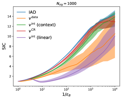
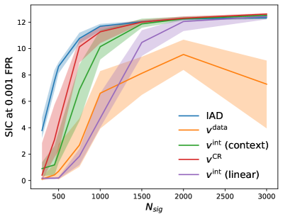
Figure 3: (Left) SIC curves for a signal injection of $1000$ (which corresponds to $S/\sqrt{B}\approx 2.2$). (Right) SIC at $\epsilon_{B}=0.001$ for different signal injections. While $v^{\rm CR}_{\theta}$ retains the best signal sensitivity, the much more computationally efficient $v^{\rm int}_{\theta}$ (context) is only a little bit worse by comparison. Meanwhile, $v^{\rm int}_{\theta}$ (linear) shows considerably worse performance at lower signal strengths.

In Fig. 3 (left), we compare the SIC curves for $N_{sig}=1000$, showing error bars for 10 different signal injections. The SIC curves for samples from $v^{\text{data}}_{\theta}(x|t,m)$ have large error bars. This is a result of the model being able to learn the full data distribution better for some signal injections (resulting in worse SIC), and so not so well in other cases (resulting in better SIC).

The weakly supervised classifier identifies both the signal and the mismodeling artifacts, evident in the pull distributions in Figure 2. At higher signal strengths the classifier is able to better identify the signal along with the mismodeling effects. At lower signal strengths, the mismodeling effects overcome the signal, which worsens the signal sensitivity. Hence $v^{\rm CR}_{\theta}$, with the best pulls in Figure 2, results in the best SIC at all signal strengths in Figure 3 (Right). Both $v^{\rm int}_{\theta}$ methods are able to interpolate out the signal, leading to an improvement over $v^{\rm data}_{\theta}$ for $N_{sig}>1500$. At lower $N_{sig}$ values, the performance of $v^{\rm int}_{\theta}$ (context) hews fairly closely to the benchmark set by $v^{\rm CR}_{\theta}$. This is significantly better than $v^{\rm int}_{\theta}$ (linear), whose performance suffers much more, due to the worse pulls shown in Figure 2.

IV Conclusions

In this work we developed SIGMA, a new and efficient interpolation method for generative modeling of backgrounds in resonant anomaly detection. Rather than needing to train separate generative models in the complement of each signal region, SIGMA re-uses a single generative model trained on all of the data, with a subsequent interpolation of its parameters from control regions into the signal region of interest. This reduces the computational cost of SIGMA significantly relative to previous approaches such as ANODE and CATHODE [3, 7], while preserving the high quality of their background templates and signal sensitivity.

The question of choosing the best interpolated background template in a data-driven way is an open one. We showed that the SIC, described in Section III, is very sensitive to bad background templates. For the LHCO R&D dataset, the $v^{\rm int}_{\theta}$ (context) method showed the best performance, only a little worse than $v^{\rm CR}_{\theta}$. However, with real data we obviously do not have access to signal and background labels to calculate the SIC with. Nevertheless, it should be possible to perform signal injection tests, as ATLAS and CMS currently do to set limits on signal models [32, 33], with artificial gaussian or other signals added to real data. One could then see first-hand whether the “all data” model learns the data plus artificial signal, and whether the interpolated versions correctly smooth out the artificial signal.

There are many interesting future directions suggested by our work. Given that there was still a small performance gap between the previous, expensive interpolation method (masking out the CR) and SIGMA, it is worthwhile to explore further improvements to our method, such as using diffusion models instead of flow-matching or performing some kind of non-linear interpolation using more than two mass points in the control region.

It would also be interesting to see how SIGMA applies to noisy features introduced in [19]. Finally, it should be totally straightforward to apply SIGMA to higher-dimensional SRs (multiple resonant features), which previously would have been even more computationally prohibitive.

Appendix A Importance of using frequency embedding

The frequency embedding is necessary for $v^{\rm data}_{\theta}$ to learn the small signal component in data. In this discussion, we denote the data model without a frequency embedding (i.e., using $\alpha(m)=m$ with $m$ being an unscaled mass) as $\tilde{v}^{\rm data}_{\theta}$. The data model with a frequency embedding, given by Equation (11), is denoted as $v^{\rm data}_{\theta}$.

As seen in Figure 4, without signal injection, both $v^{\rm data}_{\theta}$ and $\tilde{v}^{\rm data}_{\theta}$ give a SIC very close to the IAD. With the signal injection, this SIC worsens for both models. $v^{\rm data}_{\theta}$ learns the signal better and hence shows worse SIC values than $\tilde{v}^{\rm data}_{\theta}$.

For our method to be fully signal-model agnostic, we do not want the data model to smoothen out parts of the data distribution that could be relevant to the background template. Hence it is crucial that we start with the best possible data model, which in this case is the model with a frequency embedding.

Appendix B Classifier Test

To better understand what the models learned, we study the weight distributions from the classifier test introduced in [38]. We train an ensemble of 50 HistGradientBoostingClassifier classifiers to distinguish the samples from each model vs the true background samples. Hence the weight distributions show:

$$\text{weight}(x)=\frac{p_{\text{samples}}(x)}{p_{\text{background}}(x)}.$$ (15)

If model $v^{\text{data}}_{\theta}$ does learn the signal, we expect the samples after a cut $\text{weight}(x)>1$ to look like the signal. Whereas a similar cut on samples from $v^{\text{CR}}_{\theta}$ or $v^{\text{int}}_{\theta}$ should not look like the signal and should correspond to modeling between the interpolated samples and the background.

We see that $v^{\rm CR}_{\theta}$ has the best AUC, and $v^{\rm int}_{\theta}$ (linear) has the worst AUC. $v^{\rm int}_{\theta}$ (context) and $v^{\rm data}_{\theta}$ has similar AUCs, but in Fig. 5 for samples from $v^{\text{data}}_{\theta}$, the weight distribution has a long tail for $\text{weight}>1$. The resulting samples from $v^{\text{data}}_{\theta}$ after a cut $\log(\text{weight})>0.1$ in Figure 6 show the peaks where the signal is localized, as expected. The interpolated samples after the same cut don’t show the signal. This shows that $v^{\text{int}}_{\theta}$ is able to remove the signal. For $\Delta R$ samples after a cut, $v^{\rm int}_{\theta}$ (linear) shows the mismodeling artifacts which are also visible in pull distributions in Figure 2.

Figure 4: The SIC curve for background template obtained $v^{\rm data}_{\theta}$ (in black, solid) and $\tilde{v}^{\rm data}_{\theta}$ (in black, dotted), trained on data without signal injection are similar to IAD. However, comparing the same models when trained with signal injection, show that the SIC for $v^{\rm data}_{\theta}$ (with frequency embedding), is worse than $\tilde{v}^{\rm data}_{\theta}$ (without frequency embedding). This is because $v^{\rm data}_{\theta}$ learns the small signal component in data, better than $\tilde{v}^{\rm data}_{\theta}$. Hence, the frequency embedding is crucial for the model to best learn the data.

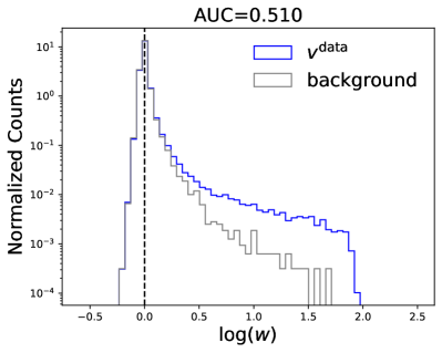
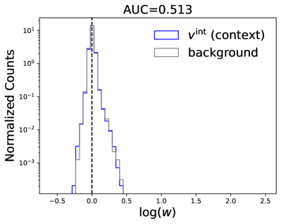
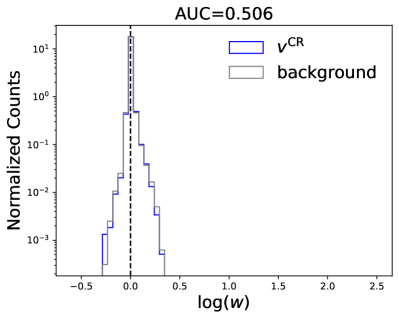
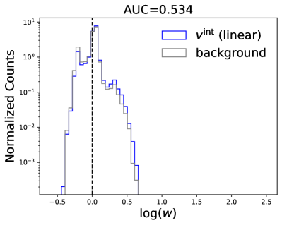
Figure 5: The weight distributions for classifier trained on samples from $v^{\text{data}}$ (Top Left)/ $v^{\text{CR}}$ (Bottom Left)/ $v^{\text{int}}$ (context) (Top Right)/ $v^{\text{int}}$ (linear) (Bottom Right) vs true background. The AUC of $v^{\rm int}_{\theta}$ (context) is slightly worse than $v^{\rm data}_{\theta}$, which produces a long tail for $\log(\text{weight})>0$ corresponding to the signal.

.

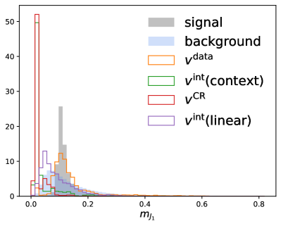
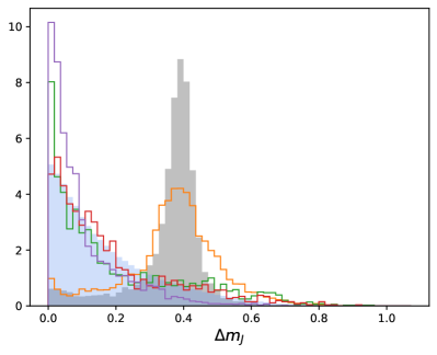
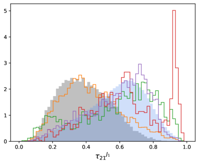
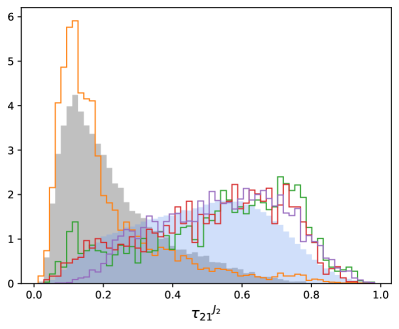
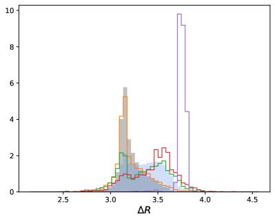
Figure 6: For $N_{sig}=3000$ and $m\in\text{SR}$, this figure shows the histograms of the samples of the features after a classifier cut $\log\text{weight}>0.1$. For $\Delta R$, we chose a higher cut $\log\text{weight}>0.2$. After a cut, we see that the samples from $v^{\text{data}}$ (in orange) are localized around the signal. This shows that the model was able to learn the signal. The samples from $v^{\rm int}_{\theta}$ (context), $v^{\rm int}_{\theta}$ (linear) and $v^{\rm CR}_{\theta}$ do not show the signal. The samples from $v^{\rm int}_{\theta}$ after a cut look similar to the other background templates, except for $\Delta R$, where the classifier finds the mismodeling artifacts.

References

- Collins et al. [2018] J. H. Collins, K. Howe, and B. Nachman, Phys. Rev. Lett. 121, 241803 (2018), arXiv:1805.02664 [hep-ph] .
- Collins et al. [2019] J. H. Collins, K. Howe, and B. Nachman, Phys. Rev. D99, 014038 (2019), arXiv:1902.02634 [hep-ph] .
- Nachman and Shih [2020] B. Nachman and D. Shih, Physical Review D 101 (2020), 10.1103/physrevd.101.075042.
- Andreassen et al. [2020] A. Andreassen, B. Nachman, and D. Shih, Phys. Rev. D 101, 095004 (2020), arXiv:2001.05001 [hep-ph] .
- Stein et al. [2020] G. Stein, U. Seljak, and B. Dai, in 34th Conference on Neural Information Processing Systems (2020) arXiv:2012.11638 [cs.LG] .
- Amram and Suarez [2020] O. Amram and C. M. Suarez, (2020), 10.1007/JHEP01(2021)153, arXiv:2002.12376 [hep-ph] .
- Hallin et al. [2022] A. Hallin, J. Isaacson, G. Kasieczka, C. Krause, B. Nachman, T. Quadfasel, M. Schlaffer, D. Shih, and M. Sommerhalder, Physical Review D 106 (2022), 10.1103/physrevd.106.055006.
- Collins et al. [2021] J. H. Collins, P. Martín-Ramiro, B. Nachman, and D. Shih, (2021), arXiv:2104.02092 [hep-ph] .
- Benkendorfer et al. [2020] K. Benkendorfer, L. L. Pottier, and B. Nachman, Phys.Rev.D 104, 035003 (2020), arXiv:2009.02205 [hep-ph] .
- Kasieczka et al. [2021a] G. Kasieczka, B. Nachman, and D. Shih (2021) arXiv:2107.02821 [stat.ML] .
- Hallin et al. [2023a] A. Hallin, G. Kasieczka, T. Quadfasel, D. Shih, and M. Sommerhalder, Phys. Rev. D 107, 114012 (2023a), arXiv:2210.14924 [hep-ph] .
- Chen et al. [2023] M. F. Chen, B. Nachman, and F. Sala, JHEP 07, 188 (2023), arXiv:2212.10579 [hep-ph] .
- Kamenik and Szewc [2023] J. F. Kamenik and M. Szewc, Phys. Lett. B 840, 137836 (2023), arXiv:2210.02226 [hep-ph] .
- Sengupta et al. [2023a] D. Sengupta, S. Klein, J. A. Raine, and T. Golling, (2023a), arXiv:2305.04646 [hep-ph] .
- Raine et al. [2023a] J. A. Raine, S. Klein, D. Sengupta, and T. Golling, Front. Big Data 6, 899345 (2023a), arXiv:2203.09470 [hep-ph] .
- Golling et al. [2023a] T. Golling, G. Kasieczka, C. Krause, R. Mastandrea, B. Nachman, J. A. Raine, D. Sengupta, D. Shih, and M. Sommerhalder, (2023a), arXiv:2307.11157 [hep-ph] .
- Golling et al. [2023b] T. Golling, S. Klein, R. Mastandrea, and B. Nachman, Physical Review D 107 (2023b), 10.1103/physrevd.107.096025.
- Bickendorf et al. [2023] G. Bickendorf, M. Drees, G. Kasieczka, C. Krause, and D. Shih, “Combining Resonant and Tail-based Anomaly Detection,” (2023), arXiv:2309.12918 [hep-ph] .
- Finke et al. [2023] T. Finke, M. Hein, G. Kasieczka, M. Krämer, A. Mück, P. Prangchaikul, T. Quadfasel, D. Shih, and M. Sommerhalder, “Back to the roots: Tree-based algorithms for weakly supervised anomaly detection,” (2023), arXiv:2309.13111 [hep-ph] .
- Freytsis et al. [2023] M. Freytsis, M. Perelstein, and Y. C. San, “Anomaly detection in presence of irrelevant features,” (2023), arXiv:2310.13057 [hep-ph] .
- Buhmann et al. [2023a] E. Buhmann, C. Ewen, G. Kasieczka, V. Mikuni, B. Nachman, and D. Shih, “Full phase space resonant anomaly detection,” (2023a), arXiv:2310.06897 [hep-ph] .
- Das et al. [2023a] R. Das, G. Kasieczka, and D. Shih, “Residual anode,” (2023a), arXiv:2312.11629 [hep-ph] .
- Beauchesne et al. [2024] H. Beauchesne, Z.-E. Chen, and C.-W. Chiang, JHEP 02, 138 (2024), arXiv:2312.06152 [hep-ph] .
- Sengupta et al. [2023b] D. Sengupta, M. Leigh, J. A. Raine, S. Klein, and T. Golling, “Improving new physics searches with diffusion models for event observables and jet constituents,” (2023b), arXiv:2312.10130 [physics.data-an] .
- Kasieczka et al. [2021b] G. Kasieczka, B. Nachman, D. Shih, O. Amram, A. Andreassen, K. Benkendorfer, B. Bortolato, G. Brooijmans, F. Canelli, J. H. Collins, B. Dai, F. F. De Freitas, B. M. Dillon, I.-M. Dinu, Z. Dong, J. Donini, J. Duarte, D. A. Faroughy, J. Gonski, P. Harris, A. Kahn, J. F. Kamenik, C. K. Khosa, P. Komiske, L. Le Pottier, P. Martín-Ramiro, A. Matevc, E. Metodiev, V. Mikuni, C. W. Murphy, I. Ochoa, S. E. Park, M. Pierini, D. Rankin, V. Sanz, N. Sarda, U. Seljak, A. Smolkovic, G. Stein, C. M. Suarez, M. Szewc, J. Thaler, S. Tsan, S.-M. Udrescu, L. Vaslin, J.-R. Vlimant, D. Williams, and M. Yunus, Reports on Progress in Physics 84, 124201 (2021b).
- Sengupta et al. [2023c] D. Sengupta, S. Klein, J. A. Raine, and T. Golling, “Curtains flows for flows: Constructing unobserved regions with maximum likelihood estimation,” (2023c), arXiv:2305.04646 [hep-ph] .
- Mastandrea and Nachman [2022] R. Mastandrea and B. Nachman, in 36th Conference on Neural Information Processing Systems (2022) arXiv:2212.06155 [hep-ph] .
- Cheng et al. [2024] C. L. Cheng, G. Singh, and B. Nachman, (2024), arXiv:2405.08889 [hep-ph] .
- Benkendorfer et al. [2021] K. Benkendorfer, L. Le Pottier, and B. Nachman, Physical Review D 104 (2021), 10.1103/physrevd.104.035003.
- Leigh et al. [2024] M. Leigh, D. Sengupta, B. Nachman, and T. Golling, “Accelerating template generation in resonant anomaly detection searches with optimal transport,” (2024), arXiv:2407.19818 [hep-ph] .
- Li et al. [2024] C. Li et al., (2024), arXiv:2405.12972 [hep-ph] .
- Aad et al. [2020] G. Aad et al. (ATLAS), Phys. Rev. Lett. 125, 131801 (2020), arXiv:2005.02983 [hep-ex] .
- CMS [2024] Model-agnostic search for dijet resonances with anomalous jet substructure in proton-proton collisions at = 13 TeV, Tech. Rep. (CERN, Geneva, 2024).
- Shih et al. [2021] D. Shih, M. R. Buckley, L. Necib, and J. Tamanas, Monthly Notices of the Royal Astronomical Society 509, 5992–6007 (2021).
- Shih et al. [2023] D. Shih, M. R. Buckley, and L. Necib, “Via machinae 2.0: Full-sky, model-agnostic search for stellar streams in gaia dr2,” (2023), arXiv:2303.01529 [astro-ph.GA] .
- Pettee et al. [2023] M. Pettee, S. Thanvantri, B. Nachman, D. Shih, M. R. Buckley, and J. H. Collins, Monthly Notices of the Royal Astronomical Society 527, 8459 (2023), https://academic.oup.com/mnras/article-pdf/527/3/8459/54646050/stad3663.pdf .
- Sengupta et al. [2024] D. Sengupta, S. Mulligan, D. Shih, J. A. Raine, and T. Golling, “Skycurtains: Model agnostic search for stellar streams with gaia data,” (2024), arXiv:2405.12131 [astro-ph.GA] .
- Das et al. [2023b] R. Das, L. Favaro, T. Heimel, C. Krause, T. Plehn, and D. Shih, “How to understand limitations of generative networks,” (2023b), arXiv:2305.16774 [hep-ph] .
- Kasieczka et al. [2022] G. Kasieczka, B. Nachman, and D. Shih, “R&D Dataset for LHC Olympics 2020 Anomaly Detection Challenge,” (2022).
- Kasieczka et al. [2021c] G. Kasieczka, B. Nachman, D. Shih, et al., Rept. Prog. Phys. 84, 124201 (2021c), arXiv:2101.08320 [hep-ph] .
- Sjöstrand et al. [2006] T. Sjöstrand, S. Mrenna, and P. Skands, Journal of High Energy Physics 2006, 026–026 (2006).
- Sjöstrand et al. [2008] T. Sjöstrand, S. Mrenna, and P. Skands, Computer Physics Communications 178, 852–867 (2008).
- de Favereau et al. [2014] J. de Favereau, C. Delaere, P. Demin, A. Giammanco, V. Lemaître, A. Mertens, and M. Selvaggi, Journal of High Energy Physics 2014 (2014), 10.1007/jhep02(2014)057.
- Mertens [2015] A. Mertens, Journal of Physics: Conference Series 608, 012045 (2015).
- Selvaggi [2014] M. Selvaggi, Journal of Physics: Conference Series 523, 012033 (2014).
- Cacciari and Salam [2006] M. Cacciari and G. P. Salam, Physics Letters B 641, 57–61 (2006).
- Cacciari et al. [2008] M. Cacciari, G. P. Salam, and G. Soyez, Journal of High Energy Physics 2008, 063–063 (2008).
- Cacciari et al. [2012] M. Cacciari, G. P. Salam, and G. Soyez, The European Physical Journal C 72 (2012), 10.1140/epjc/s10052-012-1896-2.
- Thaler and Van Tilburg [2011] J. Thaler and K. Van Tilburg, Journal of High Energy Physics 2011 (2011), 10.1007/jhep03(2011)015.
- Thaler and Van Tilburg [2012] J. Thaler and K. Van Tilburg, Journal of High Energy Physics 2012 (2012), 10.1007/jhep02(2012)093.
- Raine et al. [2023b] J. A. Raine, S. Klein, D. Sengupta, and T. Golling, Frontiers in Big Data 6 (2023b), 10.3389/fdata.2023.899345.
- Shih [2021] D. Shih, “Additional QCD Background Events for LHCO2020 R&D (signal region only),” (2021).
- Lipman et al. [2023] Y. Lipman, R. T. Q. Chen, H. Ben-Hamu, M. Nickel, and M. Le, “Flow matching for generative modeling,” (2023), arXiv:2210.02747 [cs.LG] .
- Birk et al. [2023] J. Birk, E. Buhmann, C. Ewen, G. Kasieczka, and D. Shih, “Flow matching beyond kinematics: Generating jets with particle-id and trajectory displacement information,” (2023), arXiv:2312.00123 [hep-ph] .
- Buhmann et al. [2023b] E. Buhmann, C. Ewen, D. A. Faroughy, T. Golling, G. Kasieczka, M. Leigh, G. Quétant, J. A. Raine, D. Sengupta, and D. Shih, “Epic-ly fast particle cloud generation with flow-matching and diffusion,” (2023b), arXiv:2310.00049 [hep-ph] .
- Ho et al. [2020] J. Ho, A. Jain, and P. Abbeel, “Denoising diffusion probabilistic models,” (2020), arXiv:2006.11239 [cs.LG] .
- Tong et al. [2024] A. Tong, K. Fatras, N. Malkin, G. Huguet, Y. Zhang, J. Rector-Brooks, G. Wolf, and Y. Bengio, “Improving and generalizing flow-based generative models with minibatch optimal transport,” (2024), arXiv:2302.00482 [cs.LG] .
- Pooladian et al. [2023] A.-A. Pooladian, H. Ben-Hamu, C. Domingo-Enrich, B. Amos, Y. Lipman, and R. T. Q. Chen, “Multisample flow matching: Straightening flows with minibatch couplings,” (2023), arXiv:2304.14772 [cs.LG] .
- Liu et al. [2022] X. Liu, C. Gong, and Q. Liu, “Flow straight and fast: Learning to generate and transfer data with rectified flow,” (2022), arXiv:2209.03003 [cs.LG] .
- Albergo and Vanden-Eijnden [2023] M. S. Albergo and E. Vanden-Eijnden, “Building normalizing flows with stochastic interpolants,” (2023), arXiv:2209.15571 [cs.LG] .
- Chen et al. [2019] R. T. Q. Chen, Y. Rubanova, J. Bettencourt, and D. Duvenaud, “Neural ordinary differential equations,” (2019), arXiv:1806.07366 [cs.LG] .
- He et al. [2015] K. He, X. Zhang, S. Ren, and J. Sun, “Deep residual learning for image recognition,” (2015), arXiv:1512.03385 [cs.CV] .
- Durkan et al. [2020] C. Durkan, A. Bekasov, I. Murray, and G. Papamakarios, “nflows: normalizing flows in PyTorch,” (2020).
- Hallin et al. [2023b] A. Hallin, G. Kasieczka, T. Quadfasel, D. Shih, and M. Sommerhalder, Physical Review D 107 (2023b), 10.1103/physrevd.107.114012.
- Mildenhall et al. [2020] B. Mildenhall, P. P. Srinivasan, M. Tancik, J. T. Barron, R. Ramamoorthi, and R. Ng, “Nerf: Representing scenes as neural radiance fields for view synthesis,” (2020), arXiv:2003.08934 [cs.CV] .
- Rahaman et al. [2019] N. Rahaman, A. Baratin, D. Arpit, F. Draxler, M. Lin, F. A. Hamprecht, Y. Bengio, and A. Courville, “On the spectral bias of neural networks,” (2019), arXiv:1806.08734 [stat.ML] .
- Paszke et al. [2019] A. Paszke, S. Gross, F. Massa, A. Lerer, J. Bradbury, G. Chanan, T. Killeen, Z. Lin, N. Gimelshein, L. Antiga, A. Desmaison, A. Köpf, E. Yang, Z. DeVito, M. Raison, A. Tejani, S. Chilamkurthy, B. Steiner, L. Fang, J. Bai, and S. Chintala, “Pytorch: An imperative style, high-performance deep learning library,” (2019), arXiv:1912.01703 [cs.LG] .
- Loshchilov and Hutter [2019] I. Loshchilov and F. Hutter, “Decoupled weight decay regularization,” (2019), arXiv:1711.05101 [cs.LG] .
- Rozet et al. [2022] F. Rozet et al., “Zuko: Normalizing flows in pytorch,” (2022).
- Zhuang et al. [2020] J. Zhuang, N. Dvornek, X. Li, S. Tatikonda, X. Papademetris, and J. Duncan, “Adaptive checkpoint adjoint method for gradient estimation in neural ode,” (2020), arXiv:2006.02493 [stat.ML] .