On the Origin of the High Star-Formation Efficiency in Massive Galaxies at Cosmic Dawn

Abstract

Motivated by the early excess of bright galaxies seen by JWST, we run zoom-in cosmological simulations of a massive galaxy at Cosmic Dawn (MDG), in a halo of $10^{11}M_{\odot}$ at $z=9$, using the hydro-gravitational code RAMSES at an effective resolution $\sim 10~{}{\rm pc}$. We investigate physical mechanisms that enhance the star-formation efficiencies (SFEs) under the unique conditions of high gas density ($\sim 3\times 10^{3}~{}{\rm cm^{-3}}$, $\sim 10^{4}~{}M_{\odot}/{\rm pc^{2}}$). Our fiducial star formation recipe uses a physically-motivated, turbulence-based, multi-freefall model, avoiding ad-hoc extrapolation from lower redshifts. By $z=9$, our simulated galaxy is a clumpy, thick, rotating disc with a high stellar mass of a few $10^{9}~{}M_{\odot}$ and high star formation rate of $\sim 100~{}M_{\odot}/{\rm yr}$. The high gas density makes supernova (SN) feedback less effective at suppressing star formation, producing a relatively high local SFE $\gtrsim 10\%$. The global SFE is dominated by feedback-driven outflows and is only weakly correlated with the local SFE. Photoionization heating can enhance the effects of SN feedback on the local SFE by making more SNe explode in diffuse environments, but the global SFE remains high even in our simulations with the strongest feedback. Intense accretion at Cosmic Dawn seeds strong turbulence, which reduces the local SFE for the same gas conditions due to turbulent pressure support. This prevents star-forming clouds from catastrophically collapsing, but this only weakly affects the global SFE. The star formation histories of our simulated galaxies are in the ballpark of the MDGs seen by JWST, despite our limited resolution. They set the stage for future simulations which treat radiation self-consistently and use a higher effective resolution $\sim 1~{}{\rm pc}$ which captures the physics of star-forming clouds.

1 Introduction

The James Webb Space Telescope (JWST) has opened a new frontier for empirical constraints on galaxy formation models at cosmic dawn ($z\geq 9$), an epoch starting with the formation of the first stars and ending with the reionization of the inter-galactic medium (IGM). At these redshifts, JWST’s NIRCam and NIRSpec instruments probe the rest-frame ultraviolet (UV), where they can provide estimates for stellar mass and star formation rate (SFR).

So far, JWST has found a growing list of $z\sim 10$ objects with high stellar masses $M_{*}\gtrsim 10^{8}~{}M_{\odot}$ and/or high SFRs $\dot{M}_{*}\gtrsim 1~{}M_{\odot}/{\rm yr}$ (e.g. Finkelstein et al., 2023b; Labbé et al., 2023; Mason et al., 2023; Carniani et al., 2024). These massive cosmic dawn galaxies (MDGs) form an excess in the abundance of the (UV-)brightest galaxies relative to expectations of standard galaxy formation models (Boylan-Kolchin, 2023). Shen et al. (2023) show that to reproduce the UV luminosity function (UVLF) inferred from MDGs, one requires that $\sim 30\%$ of the baryonic matter accreting onto a dark matter (DM) halo is converted into stars. This is far higher than the canonical value of $\lesssim 5\%$ for galaxies at lower redshift in a similar mass and redshift range.

The explanations for this tension fall into four categories. First, star formation might be intrinsically more efficient at Cosmic Dawn (Dekel et al., 2023). Second, a low mass-to-light ratio at Cosmic Dawn could cause models calibrated to the lower-redshift Universe to overestimate stellar masses. These explanations include the presence of AGN (Wang et al., 2024), a top-heavy stellar initial mass function (IMF) (Sharda & Krumholz, 2022; Cameron et al., 2023), a lack of dust along the line of sight (Mason et al., 2023; Ferrara et al., 2023), and differences in dust properties. Third, observations could be biased by bursty star formation at Cosmic Dawn (Sun et al., 2023; Shen et al., 2023). In this scenario, the bright end of the UVLF is dominated by less intrinsically bright galaxies which have undergone a recent burst. Finally, a modified $\Lambda$-CDM cosmology can produce a greater abundance of massive haloes at Cosmic Dawn. These explanations include “Early Dark Energy” (Klypin et al., 2021) or massive primordial black hole seeds (Liu & Bromm, 2022).

Some combination of effects may contribute to the tension. In this work, we explore the possibility that star formation is intrinsically more efficient at Cosmic Dawn. Ultimately, a change in the physics of star formation must result from differences in the properties of the interstellar medium (ISM). A key difference is that the typical density of the ISM was greater at Cosmic Dawn by a factor $\sim 1000$ due to cosmic expansion.

In Figure 1, we plot the comoving number density of dark matter haloes as a function of halo mass and redshift, assuming cosmological parameters from the Plank 2018 results (Planck Collaboration et al., 2020). We estimate the number density by integrating the Press-Schechter halo mass function (Press & Schechter, 1974) using the Python package COLOSSUS (Diemer, 2018). haloes become increasingly rare at larger masses and higher redshifts. We also plot a simple estimate for the baryon surface density of the galaxy hosted by the halo (App. A).

The MDGs seen by JWST must have number densities on the order of a few per effective JWST survey volume, which is roughly $n_{\rm halo}\sim 10^{-6}~{}(h_{0}^{-1}{\rm cMpc^{3}})^{-3}$. For example, $V_{\rm eff}(M\leq-20)\simeq 160000~{}{\rm cMpc^{3}}$ for the Cosmic Evolution Early Release Science (CEERS Finkelstein et al., 2023a, ERS-1345). Using Figure 1, this implies that at a redshift $z\sim 9$, the MDGs seen by JWST have halo masses $M_{\rm halo}\sim 10^{11}~{}M_{\rm halo}$ and baryon surface densities $\Sigma_{\rm gas}\sim 10^{4}~{}M_{\odot}/{\rm pc^{2}}$, two orders of magnitude larger than the typical surface densities in Milky Way like galaxies (Ostriker & Kim, 2022). For a disc scale height $H/R\sim 0.1$, this gives a Hydrogen number density $n_{\rm H}\sim 3\times 10^{3}~{}{\rm cm^{-3}}$. The density in star-forming regions is expected to be up to an order of magnitude higher $n_{\rm H}\sim 3\times 10^{4}~{}{\rm cm^{-3}}$.

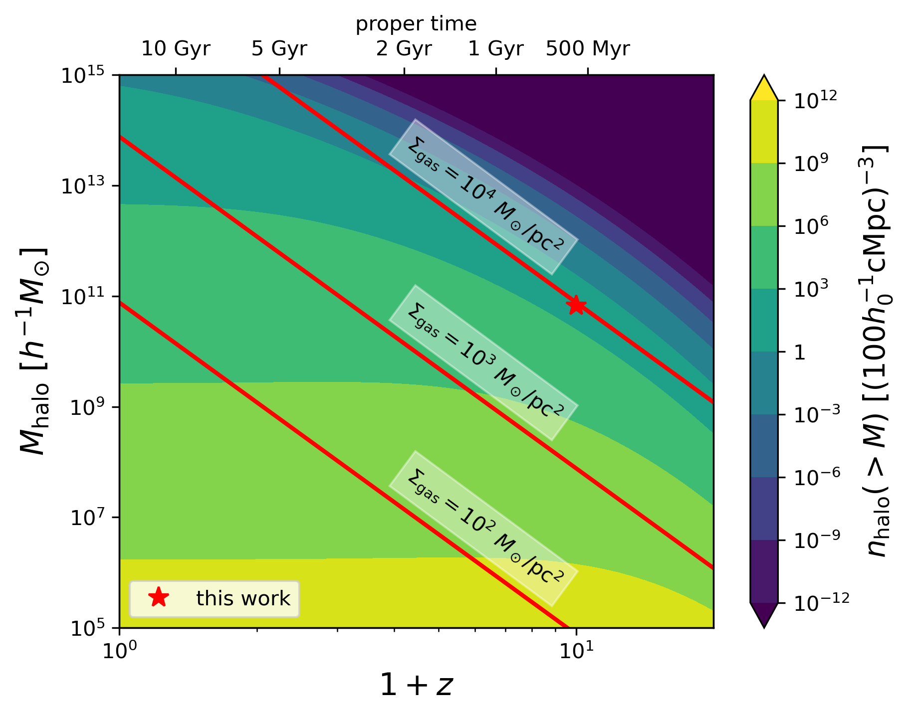
Figure 1: The comoving number density of dark matter haloes as a function of halo mass and redshift. A simple estimate for gas surface density (App. A) is used to plot lines of constant gas surface density in red. The most massive galaxies at Cosmic Dawn seen by JWST likely have number densities $n_{\rm halo}\sim 10^{-6}~{}(h_{0}^{-1}{\rm cMpc^{3}})^{-3}$. Our simulation (red star) probes galaxies with similar number densities. The high densities $\Sigma_{\rm gas}\sim 10^{4}~{}M_{\odot}/{\rm pc^{2}}$ and $n_{\rm H}\sim 3\times 10^{3}~{}{\rm cm^{-3}}$ create a unique environment for star formation which is not realized in the lower redshift Universe.

Such high densities create a unique environment for star formation which is not realized in the lower redshift Universe, except in nuclear regions of lower redshift galaxies, where the typical result is a starburst (e.g. Naab & Ostriker, 2017). This suggests that MDGs might have starburst-like SFR densities throughout their entire volume, rather than just in their center. In their feedback-free starburst (FFB) model, Dekel et al. (2023) argue that the high density conditions of Cosmic Dawn might suppress the stellar feedback processes which usually regulate star formation.

However, the physical conditions of the ISM in MDGs differs from present day galaxies in other ways too. The rapid accretion of cold streams in massive galaxies at high redshift is expected to seed strong turbulence (Dekel et al., 2009; Ginzburg et al., 2022). This is empirically supported by the high velocity dispersions observed in galaxies at $z\gtrsim 6$ de Graaff et al. (2024b). Turbulent pressure may support molecular clouds against gravitational collapse, suppressing star formation locally. Turbulence can also reduce the clustering of supernovae (SNe), making SN feedback less effective (Gentry et al., 2017). In addition to turbulence, the low metal content of the ISM and the higher CMB temperatur at Cosmic Dawn may suppress star formation by making cooling less efficient.

We capture these effects in a set of cosmological simulations from $z=100$ to $z=9$, focusing on a halo which reaches a mass $M_{\rm halo}=10^{11}~{}M_{\odot}$ at $z=9$, indicated by the red star in Figure 1. Our models vary in their treatment of turbulence and stellar feedback, allowing us to investigate how star formation on a global scale is connected to physics on a local scale.

The star formation recipe commonly used in simulations of galaxy formation defines the local SFR density $\dot{\rho}_{*}=\epsilon_{\rm ff}\rho/\tau_{\rm ff}$, where $\epsilon_{\rm ff}$ is the local star formation efficiency (SFE) per freefall time $\tau_{\rm ff}$. Typically, $\epsilon_{\rm ff}$ is set to a constant value on the order of a few percent, consistent with observations of the local Universe (e.g. Hopkins et al., 2014). However, to understand how the different physical conditions in the ISM at Cosmic Dawn affect star formation, we need a more predictive model. Our fiducial model uses a physically-motivated, turbulence-based, multi-freefall model (Federrath & Klessen, 2012), avoiding ad hoc extrapolation from lower redshifts.

This work is only the first step towards understanding the physics of star formation in MDGs. Our treatment of stellar feedback is crude due to the limitations of our effective resolution $\sim 10~{}{\rm pc}$ in a pure hydrodynamics simulation (i.e. no radiation). Therefore, our quantitative results should be taken with a grain of salt. Future work will treat radiation self-consistently and use a higher effective resolution $\sim 1~{}{\rm pc}$ which captures the physics of star-forming clouds.

In Section 2, we explain our numerical methods and our suite of models. In Section 3, we analyze our results. In Section 4, we interpret our results with toy models, discuss caveats, and discuss observational implications. We conclude in Section 5. Tangential discussions are provided in the appendices.

2 Numerical Methods

We use the adaptive mesh refinement (AMR) code RAMSES (Teyssier, 2002) to model the interaction of dark matter, star clusters, and baryonic gas in a cosmological context. We start with a discussion of the relevant technical details of RAMSES and our initial conditions (Sec. 2.1). We follow with the details of our recipes for subgrid turbulence (Sec. 2.2), star formation (Sec. 2.3), SN feedback (Sec. 2.4), and early feedback (Sec. 2.5). Finally, we describe our suite of simulations (Sec. 2.6).

2.1 RAMSES

RAMSES evolves gas quantities in an Eulerian sense on a discretized grid of cubical cells, which can be adaptively refined to increase the spatial resolution locally according to some adopted Adaptive Mesh Refinement (AMR) criterion. Dark matter and star cluster particles are evolved in a Lagrangian sense. Dark matter particles and gas cells are coupled via the Poisson equation while star cluster particles and gas cells are coupled via recipes for star formation, early feedback, and SN feedback. We adopt standard cosmological parameters $h_{0}=0.7$, $\Omega_{\rm m,0}=0.276$, $\Omega_{\rm b,0}=0.049$, $\Omega_{\Lambda,0}=0.724$, and zero curvature, consistent with current constraints.

Each particle is defined by a unique identification number (ID), a position $\mathbf{x}$ and a velocity $\mathbf{v}$. Star cluster particles carry additional metadata including their mass $m_{*}$, metallicity $Z$, and time of birth $t_{\rm birth}$. We evolve density $\rho$, pressure $P$, velocity $\mathbf{v}$, and metallicity $Z$ on the grid according to the Euler equations using the MUSCL-Hancock scheme, a second-order Godunov method, and the Harten-Lax-van Leer-Contact Leer (HLLC) Riemann solver (Harten et al., 1983). We use a fine timestep controlled by several stability conditions (see Teyssier, 2002) and whose size is roughly $\tau_{\rm fine}\simeq 500~{}{\rm yr}$.

We assume an ideal gas equation of state appropriate for a rarefied plasma with $\gamma=5/3$. The turbulent kinetic energy (TKE) $\varepsilon_{\rm turb}$ and a refinement mask $M$ are advected passively with the flow. The trajectories of dark matter and star cluster particles are computed using a particle-mesh solver. The Poisson equation is solved using a multi-grid method (Guillet & Teyssier, 2011) with Dirichlet boundary conditions at level boundaries.

The grid resolution can be defined in terms of a refinement level $\ell$ as $\Delta x=L/2^{\ell}$. Similarly, we can define the mass resolution of dark matter particles as

$$m_{\rm dm}=\Omega_{\rm m,0}\rho_{\rm crit,0}(L/2^{\ell})^{3}$$ (1)

where $\rho_{\rm crit,0}=3H_{0}^{2}/(8\pi G)$ is the critical density at $z=0$.

We generate initial conditions for a low-resolution ($\ell=9$) dark matter only simulation in a comoving volume $L^{3}=(100h_{0}^{-1}{\rm cMpc})^{3}$ at $z=100$ using MUSIC (Hahn & Abel, 2011). We run the simulation until $z=9$ and identify a candidate halo with a mass $M_{\rm halo}\simeq 10^{11}~{}M_{\odot}$. We trace the dark matter particles of the candidate halo back to their positions at $z=100$ and define the convex hull created by these particles as the zoom region.

We generate new initial conditions using MUSIC including dark matter and baryons. The simulation box is translated such that the candidate halo will form near the center of the box at $z=9$. Within the zoom region, we use a resolution $\ell=14$. Outside the zoom region, we progressively degrade the resolution until $\ell=7$, enforcing a separation of 5 cells between level boundaries (from $\ell=7$ to $\ell=14$). We refer to this initial grid as the coarse grid. We track the Lagrangian volume of the halo throughout the simulation using the refinement mask, which we set equal to unity inside the zoom region and zero otherwise.

The dark matter mass resolution in the zoom region is $m_{\rm dm,min}\simeq 2.48\times 10^{4}~{}M_{\odot}$. The corresponding baryon mass resolution is $m_{\rm b,min}=f_{\rm b}m_{\rm dm,min}\simeq 4400~{}M_{\odot}$, where $f_{\rm b}=\Omega_{\rm b,0}/\Omega_{\rm m,0}\simeq 0.17$ is the baryon fraction. As a post hoc confirmation of our approach, we have verified that all dark matter particles within a $50~{}{\rm kpc}$ sphere of the galaxy have mass $m_{\rm dm}$ throughout the duration of our simulations.

As the simulation runs, we refine the initial coarse grid based on a quasi-Lagrangian approach. A cell is refined if

1. The refinement mask $M>0.1$

and at least one of the following conditions is met:

1. The dark matter mass in a cell exceeds $8m_{\rm dm}$

2. There baryonic (gas + star) mass in a cell exceeds $8m_{\rm b}$

3. There are more than 5 Jeans lengths per cell.

Criterion (i) ensures that only cells which exchange gas with the initial zoom-in region are refined. Criterion (iv) ensures that before a cell acquires enough mass to become gravitationally unstable at a given resolution, the cell is refined. Therefore, only cells at the highest refinement level should become gravitationally unstable and form stars.

We increment the maximum refinement level $\ell_{\rm max}$ each time the physical box size doubles due to cosmic expansion, reaching $\ell_{\rm max}=20$ at expansion factor $a\in[0.05,0.1]$. This approach maintains a constant physical effective resolution $\Delta x_{\rm min}=L/2^{\ell_{\rm max}}\simeq 10~{}{\rm pc}$ throughout the duration of the simulation.

We do not directly model Pop III star formation. Instead, we enrich the ISM to $10^{-3}Z_{\odot}$ in the initial conditions. Previous simulation work shows that a single pair instability SN can enrich the host halo to at least this metallicity (Wise et al., 2011). Furthermore, this is above the critical metallicity $\sim 10^{-3.5}Z_{\odot}$ at which Pop III stars cease to form due to fine-structure Carbon and Oxygen line cooling (Bromm & Loeb, 2003). Therefore, our initial conditions are consistent with our lack of Pop III star modeling.

Gas cooling and heating is implemented using equilibrium chemistry for Hydrogen and Helium (Katz et al., 1996), with a metallicity-dependence given by Sutherland & Dopita (1993) and cosmological abundances ($X=0.76$, $Y=0.24$). In diffuse gas $n_{\rm H}\leq 0.01~{}{\rm cm^{-3}}$ (Aubert & Teyssier, 2010), we account for heating from the extragalactic UV background assuming a uniform radiation field which evolves with time according to Haardt & Madau (1996). This likely underestimates the UV background in MDGs due to clustering effects, but the error is acceptable given the simplicity of our model.

We floor the temperature at the cosmic microwave background (CMB) temperature to account for heating by CMB photons. This effect is important at Cosmic Dawn, when the CMB temperature is higher than the temperatures of star-forming clouds at the present day. When we stop our simulations at $z=9$, the CMB temperature is $T_{\rm CMB}\simeq 27.25~{}{\rm K}$.

We run our simulations on the Stellar cluster at Princeton University. Each simulation was run on 4 nodes with 96 cores per code, making 384 cores total. The cores on stellar are 2.9 GHz Intel Cascade Lake processors. Each simulation took approximately 2 weeks of runtime to reach completion.

2.2 Subgrid turbulence model

We use a Large Eddy Simulation (LES) method for subgrid turbulence similar to Kretschmer & Teyssier (2020). To describe this model, we decompose the subgrid density field $\rho$ into a bulk component $\overline{\rho}$ and a turbulent component $\rho^{\prime}$:

$$\rho=\overline{\rho}+\rho^{\prime}$$ (2)

The bulk component is defined as the volume-average density field smoothed on the scale of the cell $\Delta x$. We also decompose the subgrid temperature $T$ and velocity $\mathbf{v}$ fields into bulk components $\widetilde{T}$, $\widetilde{\mathbf{v}}$ and turbulent components $T^{\prime\prime}$, $\mathbf{v}^{\prime\prime}$:

$$T=\widetilde{T}+T^{\prime\prime},\quad\mathbf{v}=\widetilde{\mathbf{v}}+\mathbf{v}^{\prime\prime}\quad{\rm with}\quad\widetilde{T}=\frac{\overline{\rho T}}{\overline{\rho}},\quad\widetilde{\mathbf{v}}=\frac{\overline{\rho\mathbf{v}}}{\overline{\rho}}$$ (3)

The bulk components are defined as the mass-weighted volume-average fields, also known as Favre-averaged fields.

The specific TKE is defined as

$$\varepsilon_{\rm turb}=\frac{1}{2}\overline{\rho v^{\prime\prime 2}}=\frac{1}{2}\overline{\rho}\sigma_{\rm 3D}^{2}=\frac{3}{2}\overline{\rho}\sigma_{\rm 1D}^{2}$$ (4)

where $\sigma_{\rm 3D}$ (resp. $\sigma_{\rm 1D}$) is the three-dimensional (resp. one-dimensional) turbulent velocity dispersion. Using these definitions, one can derive equations for the TKE and bulk fluid components (Schmidt & Federrath, 2011; Semenov et al., 2017)

The bulk fluid equations include new terms for turbulent diffusion. However, the turbulent diffusion is generally small compared to the diffusion introduced by the numerical scheme. We maintain the original fluid equations rather than adding a diffusive term to an already too-diffusive scheme, following previous work (Schmidt et al., 2006; Kretschmer & Teyssier, 2020).

The TKE equation reads

$$\partialderivative{t}\varepsilon_{\rm turb}+\partialderivative{x_{j}}(\varepsilon_{\rm turb}\widetilde{v}_{j})+P_{\rm turb}\partialderivative{\widetilde{v}_{j}}{x_{j}}=\mathcal{C}_{\rm turb}-\mathcal{D}_{\rm turb}$$ (5)

where $P_{\rm turb}=2/3\varepsilon_{\rm turb}=\overline{\rho}\sigma_{\rm 1D}^{2}$ is the turbulent pressure and $\mathcal{C}_{\rm turb}$ and $\mathcal{D}_{\rm turb}$ are creation and destruction source terms respectively.

In the LES framework, we assume that resolved and unresolved turbulence are coupled by eddies at the resolution scale. Defining the turbulent viscosity $\mu_{\rm turb}=\overline{\rho}\Delta x\sigma_{\rm 1D}$, the turbulence creation term is

$$\mathcal{C}_{\rm turb}=2\mu_{\rm turb}\sum_{ij}\left[\frac{1}{2}\left(\partialderivative{\widetilde{v_{i}}}{x_{j}}+\partialderivative{\widetilde{v_{j}}}{x_{i}}\right)-\frac{1}{3}(\divergence{\widetilde{\mathbf{v}}})\delta_{ij}\right]=\frac{1}{2}\mu_{\rm turb}\absolutevalue{\widetilde{S}_{ij}}^{2}$$ (6)

where $\widetilde{S}$ is the bulk viscous stress tensor. Defining the turbulent dissipation timescale $\tau_{\rm diss}=\Delta x/\sigma_{\rm 1D}$, the turbulence destruction term is

$$\mathcal{D}_{\rm turb}=\frac{\varepsilon_{\rm turb}}{\tau_{\rm diss}}$$ (7)

One caveat of the LES model is that gravitational forces do not enter into the turbulence creation term (Eq. 6). In a stable Keplerian disc, gravitational forces can stabilize shear flows against the Kelvin-Helmholtz instability, so the model overestimates the TKE source term. In a gravitationally unstable disc, gravitational forces can source additional turbulence, so the model underestimates the TKE source term.

2.3 Star formation recipe

2.3.1 Subgrid density PDF

Empirically, star formation is described by the Kennicutt-Schmidt (KS) law (Kennicutt, 1998), which relates the SFR surface density and gas surface density by $\Sigma_{\rm SFR}\propto\Sigma_{\rm gas}^{1.5}$. The KS relation holds at scales as small as $1~{}{\rm kpc}$ (Kennicutt et al., 2007), supporting the idea that star formation can be modeled locally as volumetric Schmidt law

$$\dot{\rho}_{*}=\epsilon_{\rm ff}\frac{\rho}{\tau_{\rm ff}}\quad{\rm with}\quad\tau_{\rm ff}=\sqrt{\frac{3\pi}{32G\rho}}$$ (8)

where $\dot{\rho}_{*}$ is the local SFR density and $\epsilon_{\rm ff}$ is the SFE per local freefall time $\tau_{\rm ff}$. This model naturally explains the power law index of $1.5$ in the empirical KS law.

Equation 8 is often combined with a fixed density threshold to obtain a simple star formation recipe which can be used in cosmological simulations (e.g. Rasera & Teyssier, 2006). The parameter $\epsilon_{\rm ff}$ is chosen to match the observed KS law in nearby resolved galaxies, typically resulting in a value $\lesssim 5\%$. However, the SFE in the local Universe cannot necessarily be extrapolated to Cosmic Dawn. This motivates a prescriptive star formation recipe which does not rely on empirical calibration.

One approach is to consider the structure of the density field on unresolved scales $\leq\Delta x_{\rm min}\simeq 10~{}{\rm pc}$. We extrapolate the turbulence spectrum to unresolved scales assuming Burgers turbulence:

$$\sigma(\ell)=\sigma_{\rm 1D}\left(\frac{\ell}{\Delta x}\right)^{1/2}$$ (9)

where $\ell$ is the spatial scale.

The turbulence transitions from supersonic to subsonic at the sonic scale $\ell_{\rm s}$ where the turbulent velocity dispersion (Eq. 9) is equal to the sound speed. Defining the turbulent Mach number $\mathcal{M}_{\rm turb}=\sigma_{\rm 1D}/c_{\rm s}$, the sonic scale is $\ell_{s}=\Delta x/\mathcal{M}_{\rm turb}^{2}$. Below the sonic scale, density fluctuations are weak, and a gas cloud can be treated as a quasi-homogeneous region.

We assume that each parcel of gas which is gravitationally unstable on the sonic scale will eventually collapse and form stars. On intermediate scales between the sonic scale and the resolution scale, density fluctuations can be significant. The probability distribution function (PDF) of density in a supersonic turbulent medium is well-described by a log-normal distribution (Vazquez-Semadeni, 1994; Kritsuk et al., 2007):

$$p(s)=\frac{1}{\sqrt{2\pi\sigma_{s}^{2}}}\exp(-\frac{(s-\overline{s})^{2}}{2\sigma_{s}^{2}})$$ (10)

with normalization condition

$$\int_{-\infty}^{\infty}p(s)\differential s=1\quad{\rm and}\quad\int_{-\infty}^{\infty}\rho p(s)\differential s=\overline{\rho}$$ (11)

where $s=\ln(\rho/\overline{\rho})$ is the logarithmic density, $\sigma_{s}$ is its standard deviation, and $\overline{s}=-1/2\sigma_{s}^{2}$ is its mean.

Padoan & Nordlund (2011) fit a simple analytic form to $\sigma_{s}$ using non-magnetized, isothermal turbulence simulations forced by an Ornstein-Uhlenbeck process:

$$\sigma_{s}^{2}=\ln(1+b^{2}\mathcal{M}_{\rm turb}^{2})$$ (12)

The parameter $b$ describes the turbulence forcing in the simulations. For purely solenoidal (divergence-free) forcing, $b=1/3$. For purely compressive (curl-free) forcing, $b=1$. The column density PDF is also well-described by a lognormal distribution, although the dispersion is generally smaller because fluctuations are averaged out by integration along the line of sight (App. G).

2.3.2 Turbulence forcing parameter

In most of our models, we set the forcing parameter to a constant value. However, we run one experimental model where we derive the forcing parameter from the local velocity field. Using a Helmholtz decomposition, the velocity field can be represented as a curl-free term $\mathbf{v}_{\rm comp}=-\gradient{\phi}$ and divergence-free term $\mathbf{v}_{\rm sol}=\curl{\mathbf{A}}$.

$$\mathbf{v}=\mathbf{v}_{\rm comp}+\mathbf{v}_{\rm sol}=-\gradient{\phi}+\curl{\mathbf{A}}$$ (13)

Computing the Helmholtz decomposition would require a computationally expensive iterative solver on the global velocity field. Instead, we use a heuristic approach motivated by the following. Taking the divergence of Equation 13 reveals that the curl-free component of the velocity field depends only on the divergence. Similarly, taking the curl reveals that the divergence-free component of the velocity field depends only on the curl. We make a simple approximation that the magnitudes of the curl-free and divergence-free components of the velocity field are proportional to the divergence and curl respectively. This gives the following expression for ratio of power in compressive to solenoidal forcing modes:

$$\psi=\frac{P_{\rm comp}}{P_{\rm sol}}=\frac{(\divergence{\mathbf{v}})^{2}}{\norm{\curl{\mathbf{v}}}^{2}}$$ (14)

Federrath et al. (2010) fit a simple analytic form to $b_{\rm turb}$ using detailed turbulence simulations (their Eq. 23):

$$b_{\rm turb}\simeq\frac{1}{3}+\frac{2}{3}\left(\frac{\psi}{\psi+1}\right)^{3}$$ (15)

2.3.3 Star formation efficiency

Assuming that star-forming cores are homogeneous spheres with diameter $\ell_{\rm s}$ (Krumholz & McKee, 2005), the gravitational stability condition is $\alpha_{\rm vir,cl}\geq 1$, where the virial parameter $\alpha_{\rm vir,s}$ is

$$\alpha_{\rm vir,cl}=\frac{2E_{\rm kin}}{\absolutevalue{E_{\rm grav}}}=\frac{15}{\pi}\frac{c_{\rm s}^{2}+\sigma(\ell_{\rm s})^{2}}{G\rho\ell_{\rm s}^{2}}$$ (16)

The gravitational stability condition can alternatively be expressed as a condition on the density $\rho\leq rho_{\rm crit}$, where

$$\rho_{\rm crit}=\frac{15}{\pi}\frac{2c_{\rm s}^{2}\mathcal{M}_{\rm turb}^{4}}{G\Delta x}=\alpha_{\rm vir}\overline{\rho}\frac{2\mathcal{M}_{\rm turb}^{4}}{1+\mathcal{M}_{\rm turb}^{2}}$$ (17)

where

$$\alpha_{\rm vir}=\frac{15}{\pi}\frac{c_{\rm s}^{2}+\sigma_{\rm 1D}^{2}}{G\overline{\rho}\Delta x^{2}}=\frac{15}{\pi}\frac{c_{\rm s}^{2}}{G\overline{\rho}\Delta x^{2}}(1+\mathcal{M}^{2})$$ (18)

is the virial parameter of the entire cell. The critical logarithmic density is

$$s_{\rm crit}=\ln\left[\alpha_{\rm vir}\frac{2\mathcal{M}_{\rm turb}^{4}}{1+\mathcal{M}^{2}}\right]$$ (19)

By design, $s_{\rm crit}$ depends on the cell size. At higher resolutions, a larger density is required to become gravitationally unstable, but gas will naturally reach those higher densities as it collapses down to that smaller cell size.

The model breaks down when the entire cell is subsonic $\mathcal{M}_{\rm turb}\lesssim 1$ (Federrath & Klessen, 2012) and the sonic scale is larger than the resolution scale. In this case, the density PDF should be interpreted as the probability distribution for the density across the entire cell and the gravitational stability condition (Equation 16) should use the resolution scale rather than the sonic scale. We smoothly interpolate between both stability conditions by defining a modified critical logarithmic density (Kretschmer & Teyssier, 2020):

$$s_{\rm crit}=\ln\left[\alpha_{\rm vir}\left(1+\frac{2\mathcal{M}_{\rm turb}^{4}}{1+\mathcal{M}_{\rm turb}^{2}}\right)\right]$$ (20)

If each gas parcel that does not meet the stability condition collapses in one freefall time and converts all its mass into stars, then the local SFR is given by

$$\dot{\rho}_{*}=\int_{s_{\rm crit}}^{\infty}\frac{\rho}{\tau_{\rm ff}(\rho)}p(s)\differential s=\epsilon_{\rm ff}\frac{\overline{\rho}}{\tau_{\rm ff}(\overline{\rho})}$$ (21)

where $\epsilon_{\rm ff}$ is the local SFE per freefall time given by

$$\begin{split}\epsilon_{\rm ff}=\ &\int_{s_{\rm crit}}^{\infty}\frac{\tau_{\rm ff}(\overline{\rho})}{\tau_{\rm ff}(\rho)}\frac{\rho}{\overline{\rho}}p(s)\differential s\\ =\ &\frac{1}{2}\exp(\frac{3}{8}\sigma_{s}^{2})\left[1+{\rm erf}\left(\frac{\sigma_{s}^{2}-s_{\rm crit}}{\sqrt{2\sigma_{s}^{2}}}\right)\right]\end{split}$$ (22)

For notational convenience, we drop the diacritical marks on the bulk fluid components for the remainder of the paper.

This is the multi-freefall (MFF) model of Federrath & Klessen (2012). This recipe is an important first step towards predictive models at Cosmic Dawn. However, there are several caveats. The model neglects deviations from a lognormal density PDF, the spatial correlation of the density field, and the timescale required to replenish the density PDF after a star has formed. Some of these issues are addressed by the recent turbulent support (TS) model of Hennebelle et al. (2024) (Sec. 4.6).

The MFF model implies that as the turbulence forcing becomes more solenoidal, the subgrid density PDF becomes more narrow (Eq. 12), generally reducing the local SFE for the same gas conditions and TKE (Eq. 22). We leave further discussion to Section 4.4.

The expected amount of star cluster particles to form in one timestep is

$$\expectationvalue{N_{\rm cl}}=\frac{\dot{\rho}_{*}\Delta x^{3}\Delta t}{M_{\rm cl}}$$ (23)

where $M_{\rm cl}$ is the star cluster particle mass. In our simulations, the fiducial value $M_{\rm cl}=M_{\rm b,min}=4400~{}M_{\odot}$ is the minimum baryon mass resolution on the coarse grid defined in Section 2.1. We draw the number of star cluster particles to form from a Poisson distribution with a Poisson parameter $\expectationvalue{N_{\rm cl}}$. This procedure allows us to model star formation as discrete events distributed in time, independent of the adopted star cluster particle mass.

Although our star formation recipe is independent of the adopted star cluster particle mass, our recipe for photoionization feedback is not. By adjusting the star particle mass, we adjust the efficiency of photoionization feedback (Sec. 2.5). We exploit this effect in our early feedback series (Sec. 2.6).

2.4 Supernovae recipe

SN explosions are one of the key feedback processes which regulate star formation. As the SFR increases, the SN rate increases commensurately. SNe inject energy and momentum into the ISM, depleting the reservoir of cold gas available to form stars.

Our simulation duration $\sim 550~{}{\rm Myr}$ is shorter than the timescales required for Type Ia SNe $\gtrsim 1~{}{\rm Gyr}$, associated with the explosion of a white dwarf in a close binary system (Tinsley, 1979). We only model Type II SNe, associated with the explosions of massive stars $m_{*}\gtrsim 8~{}M_{\odot}$.

Type II SNe are expected to occur during a window of time from $\tau_{\rm start}\simeq 3{\rm Myr}$ to $\tau_{\rm end}\simeq 20~{}{\rm Myr}$ after the birth of a massive star. These values for $\tau_{\rm start}$ and $\tau_{\rm end}$ are consistent with previous work using the population synthesis code Starburst99 (Leitherer et al., 1999; Kimm et al., 2015).

Each star cluster particle is expected to produce a number of SNe given by

$$N_{\rm SNe}=\frac{\chi M_{\rm cl}}{m_{\rm big}}$$ (24)

where $M_{\rm cl}$ is the mass of the star cluster particle, $m_{\rm big}$ is the typical mass of a massive star, and $\chi$ is the mass fraction of massive stars within the stellar population. $m_{\rm big}$ and $\chi$ are related to the IMF $\xi(m)$ via

$$m_{\rm big}=\frac{\int_{8M_{\odot}}^{\infty}m\xi(m)\differential m}{\int_{8M_{\odot}}^{\infty}\xi(m)\differential m},\quad\chi=\frac{\int_{8M_{\odot}}^{\infty}m\xi(m)\differential m}{\int_{-\infty}^{\infty}m\xi(m)\differential m}$$ (25)

Our choice of $m_{\rm big}$ and $\chi$ are the only way in which the IMF enters into our modeling. Otherwise, our model implicitly assumes that our star cluster particles fully sample the IMF. Using a Chabrier IMF (Chabrier, 2003), one finds $m_{\rm big}\simeq 19~{}M_{\odot}$ and $\chi\simeq 0.19$. We adopt $m_{\rm big}=10~{}M_{\odot}$ and $\chi=0.2$, producing somewhat more SNe than would be predicted by the Chabrier IMF, but only by a small factor well within the uncertainties of the IMF at Cosmic Dawn.

In each simulation timestep, we compute the SN rate assuming that the $N_{\rm SNe}$ events are uniformally distributed in the interval between $\tau_{\rm start}$ and $\tau_{\rm end}$:

$$\dot{N}_{\rm SNe}=\frac{N_{\rm SNe}}{\tau_{\rm end}-\tau_{\rm start}}$$ (26)

although physically, the SN distribution should be skewed towards later times (Sec. 4.7).

Multiplying by the fine timestep $\Delta t$, we obtain the expected number of SN events per timestep $\expectationvalue{N_{\rm SNe}}=\dot{N}_{\rm SNe}\Delta t$. We draw the number of SN events from a Poisson distribution with a Poisson parameter $\lambda=\expectationvalue{N_{\rm SNe}}$, similar to Hopkins et al. (2018). This procedure allows us to model SNe as discrete events distributed in time, independent of the adopted star cluster particle mass.

The an exploding SN blastwave interacts with the surrounding medium in 4 stages. Initially, the SN ejecta expands freely. Once the ejecta has swept up a mass in the ISM comparable to its own, a shock forms and expands following the Sedov-Taylor solution, approximately conserving energy. Eventually, radiative cooling behind the shock front causes the expansion to deviate from the Sedov-Taylor solution, and the expansion proceeds approximately conserving momentum. Finally, the blast wave slows due to radiative losses and accumulated material, fading into the ISM. The transition radius between the second Sedov-Taylor phase and the third “snowplow” phase is called the cooling radius.

Ideally, one should resolve the energy-conserving Sedov-Taylor phase and model a SN explosion by injecting a thermal energy $E_{\rm SN}\simeq 10^{51}~{}{\rm erg}$ into the surrounding gas. However, at high densities, the cooling radius is often smaller than the resolution scale. In this case, injecting energy into the surrounding gas would result in the energy from the SN being artificially radiated away before it could accelerate gas in the snowplow phase. To compensate for this effect, we inject momentum in addition to thermal energy when the cooling radius is not resolved. This method, known as momentum feedback, is used frequently in galaxy formation simulations (Hopkins et al., 2011, 2018; Kim & Ostriker, 2015; Kimm et al., 2015).

Martizzi et al. (2015) fit power laws in density and metallicity to the cooling radius $R_{\rm cool}$ and the SN terminal momentum $P_{\rm SN}$ using high-resolution simulations of individual SN explosions:

$$R_{\rm cool}=\ 3.0~{}{\rm pc}\left(\frac{Z}{Z_{\odot}}\right)^{-0.082}\left(\frac{n_{\rm H}}{100~{}{\rm cm^{-2}}}\right)^{-0.42}$$ (27)

$$P_{\rm SN}=\ 1.42\times 10^{5}~{}{\rm km/s}M_{\odot}\left(\frac{Z}{Z_{\odot}}\right)^{-0.137}\left(\frac{n_{\rm H}}{100~{}{\rm cm^{-2}}}\right)^{-0.16}$$ (28)

We use these equations to estimate $R_{\rm cool}$ and $P_{\rm SN}$ and inject momentum according to

$$P=P_{\rm SN}N_{\rm SN}\begin{cases}1&R_{\rm cool}<\Delta x_{\rm min}\\ (\Delta x_{\rm min}/R_{\rm cool})^{3/2}&\Delta x_{\rm min}<R_{\rm cool}<4\Delta x_{\rm min}\\ 0&R_{\rm cool}>\Delta x_{\rm min}\end{cases}$$ (29)

Our approach is only an approximation of the full model recommended by Martizzi et al. (2015), which incorporates additional physical scales into the calculation of injected momentum and energy. Martizzi et al. (2015) also provide versions of Eqs. 27 and 28 for SN which occur in an inhomogeneous medium with $\mathcal{M}_{\rm turb}=30$. In an inhomogeneous medium, the cooling radius is larger by a factor of a few because the blast wave preferentially moves through low-density channels, but the terminal energy and momentum deposited in the ISM by the SN remnant do not change significantly. Ideally, one should use a model which depends continuously on the turbulent Mach number, no such model is available at the time of writing.

We inject momentum onto the grid by dividing the momentum flux $P\Delta x^{-2}\Delta t^{-1}$ equally between the six faces of the cell and directly adding it to the thermal pressure in the Riemann solver (Agertz et al., 2013). We remove the associated $P\differential V$ work in the internal energy equation to avoid spurious heating (Kretschmer & Teyssier, 2020). We inject thermal energy onto the grid by adding $E=N_{\rm SN}E_{\rm SN}$ to the thermal energy of the cell in which the SN event occurs. We assume a SN metal yield $y=0.1$, so each SN event deposits a mass $yN_{\rm SN}m_{\rm big}=N_{\rm SN}M_{\odot}$ of metals into the ISM.

Although momentum feedback approximates the net effect of SNe on the surrounding ISM, it does not accurately model the effect of SNe on the surrounding ISM on short timescales. Therefore, our results concerning SN feedback should be considered with caution, despite our physically-motivated subgrid prescription (Sec. 4.7).

2.5 Early feedback recipe

In addition to SN feedback, stellar feedback includes thermal pressure from photoionized gas, stellar winds, radiation pressure from FUV photons, and radiation pressure from multiply-scattered IR photons reprocessed by dust. We call these early feedback processes because they begin immediately after a massive star forms, in contrast to SN feedback. Out of these feedback processes, we only model thermal pressure from photoionized gas. We discuss the effects of other early feedback processes in Section 4.5.

In each cell containing a star cluster particle younger than $\tau_{\rm end}=20~{}{\rm Myr}$, we set the temperature to $T_{\rm phot}=20000~{}{\rm K}$. This forces the gas into a fast cooling regime where it approaches the photoionization temperature within a few timesteps. In practice, we achieve this by injecting a thermal energy associated with a sound speed

$$c_{\rm s}=\sqrt{\frac{\gamma k_{\rm B}T_{\rm phot}}{\mu m_{\rm p}}}\simeq 22~{}{\rm km/s}$$ (30)

where we have assumed a $\gamma$ = 5/3 adiabatic equation of state and mean molecular weight $\mu=0.6$, appropriate for an ionized monoatomic gas.

Unlike our SN recipe, our early feedback recipe depends on the choice of $M_{\rm cl}$ because each star cluster particle has the same effect on its parent cell, regardless of its mass. If the adopted $M_{\rm cl}$ is small, then the stellar mass will be represented by a large number of star cluster particles which each photoionize their parent cell, representing efficient photoionization feedback. If the adopted $M_{\rm cl}$ is large, then the stellar mass will be represented by a small number of star cluster particles, representing inefficient photoionization feedback. $M_{\rm cl}$ should be chosen according to the stellar mass required to photoionize a cell. In this case, a star cluster particle is formed exactly when its HII region becomes resolved.

Let $\expectationvalue{Q/m_{*}}$ be the average rate of Hydrogen-ionizing photons emitted per stellar mass. This can be derived from the IMF $\xi(m)$ if the rate of ionizing photon emission $Q(m)$ is known as a function mass:

$$\expectationvalue{\frac{Q}{m_{*}}}=\frac{\int Q(m)\xi(m)\differential m}{\int m\xi(m)\differential m}$$ (31)

Using data for main sequence stars given by Table 15.1 of Draine (2011), we fit $Q(m)$ to a simple analytic form for masses $M\geq 15.6~{}M_{\odot}$ (App. B):

$$Q(m)\sim\left[8.37\times 10^{45}\left(\frac{m}{M_{\odot}}\right)^{2.12}-2.33\times 10^{48}\right]~{}{\rm cm^{-2}s^{-1}}$$ (32)

Assuming a Chabrier IMF (Chabrier, 2003), we estimate $\expectationvalue{Q/m_{*}}=5.85\times 10^{46}~{}{\rm cm^{-2}s^{-1}M_{\odot}^{-1}}$. Higher mass stars contribute more ionizing photons, but have a lower abundance. In our calculation, most of the contribution to the ionizing photons comes from stars $M_{*}\simeq 35~{}M_{\odot}$. Star clusters which are too small to sample the IMF up to this mass may have lower ionization rates.

Equating the rates of photoionization and radiative recombination, we find the classic result from Strömgren (1939) that the star cluster creates a Strömgren sphere of ionized gas with radius

$$R_{\rm S}=\left(\frac{3M_{\rm cl}}{4\pi\alpha_{B}n_{\rm H}^{2}}\expectationvalue{\frac{Q}{m_{*}}}\right)^{1/3}$$ (33)

where $\alpha_{B}\simeq 2.58\times 10^{-13}~{}{\rm cm^{3}/s}$ is the case B recombination rate at an electron temperature $T_{\rm e}=10^{4}~{}{\rm K}$ (Ferland et al., 1992). We use the on-the-spot approximation, assuming that electrons which recombine directly to the ground state do not contribute to the net ionization.

The stellar mass required to photoionize a cell is given by equating Strömgren sphere and cell volumes and solving for the star cluster mass, which yields

$$\begin{split}M_{\rm cl}=\ &\frac{4\pi}{3}\frac{\alpha_{B}n_{\rm H}^{2}\Delta x_{\rm min}^{3}}{\expectationvalue{Q/m_{*}}}\\ \simeq\ &5000~{}M_{\odot}\left(\frac{n_{\rm H}}{100~{}{\rm cm^{-2}}}\right)^{2}\left(\frac{\Delta x}{10~{}{\rm pc}}\right)^{3}\left(\frac{\expectationvalue{Q/m_{*}}~{}{\rm cm^{2}sM_{\odot}}}{5.85\times 10^{-6}}\right)^{-1}\end{split}$$ (34)

In MDGs, stars may form at significantly higher densities than the value $n_{\rm H}\sim 10^{2}~{}{\rm cm^{-2}}$ which appears in Equation 34. However, the strong turbulence in MDGs lowers the effective density relevant for photoionization because photoionizing photons preferentially escape through low-density channels in the gas. We can estimate the effective density using a Rosseland-like averaging

$$\rho_{\rm eff}=\left[\int\frac{1}{\rho}p(s)\differential s\right]^{-1}=e^{-\sigma_{s}^{2}}\overline{\rho}=\frac{\overline{\rho}}{1+b_{\rm turb}^{2}\mathcal{M}_{\rm turb}^{2}}$$ (35)

A similar concept of effective density was used in Appendix B of (Faucher-Giguère et al., 2013). For a mean density $\sim 10^{4}~{}{\rm cm^{-2}}$ and a turbulent Mach number $\sim 10$, the effective density is indeed on the order of $\sim 10^{2}~{}{\rm cm^{-2}}$.

Equation 34 gives an order-of-magnitude estimate for an appropriate star cluster particle mass in our simulation. However, it depends sensitively on density, which our simple model cannot account for. Due to the steep density dependence and the uncertainty in $\expectationvalue{Q/m_{*}}$, we vary $M_{\rm cl}$ by over an order of magnitude in different simulations (Sec. 2.6). Although crude, this model provides a rough approximation for the effect of early feedback, and will be improved upon in future work.

One caveat of this model is that we do not properly account for multiple star cluster particles in a cell. If one star cluster particle photoionizes a cell, then by the Strömgren sphere argument, multiple star particles should photoionize a region larger than a cell. In our simulations, these situations are instead handled by multiplying the injected thermal energy by the number of star cluster particles, artificially restricting the Strömgren sphere to the cell size.

2.6 The suite of simulations

Feedback series
Name	$M_{\rm cl}$ [$M_{\odot}$]	$b_{\rm turb}$	$\tau_{\rm start}$ [${\rm Myr}$]	MFF?	Phot?	SN fbk?	$M_{*}$ [$10^{9}M_{\odot}$]	${\rm SFR}_{50}$ [${\rm M_{\odot}/{\rm yr}}$]	$\epsilon_{\rm int}$	${\rm med}(\epsilon_{\rm ff})$	$\eta$
yesFbk∗	$4400$	$1.0$	$3.0$	yes	yes	yes	$3.52$	$144.3$	19.8%	$13.8\%$	$1.39$
SNeOnly	$880$	$1.0$	$3.0$	yes	no	yes	$6.03$	$293.6$	33.9%	$20.2\%$	$0.50$
photOnly	$4400$	$1.0$	$3.0$	yes	yes	no	$9.16$	$349.2$	51.6%	$17.7\%$	$0.03$
noFbk	$4400$	$1.0$	$3.0$	yes	no	no	$9.20$	$352.1$	51.8%	$18.1\%$	$0.03$
Early feedback series
Name	$M_{\rm cl}$ [$M_{\odot}$]	$b_{\rm turb}$	$\tau_{\rm start}$ [${\rm Myr}$]	MFF?	Phot?	SN fbk?	$M_{*}$ [$10^{9}M_{\odot}$]	${\rm SFR}_{50}$ [${\rm M_{\odot}/{\rm yr}}$]	$\epsilon_{\rm int}$	${\rm med}(\epsilon_{\rm ff})$	$\eta$
highPhot	$880$	$1.0$	$3.0$	yes	yes	yes	$1.81$	$53.7$	$10.2\%$	$7.2\%$	$10.1$
medPhot∗	$4400$	$1.0$	$3.0$	yes	yes	yes	$3.52$	$144.3$	$19.8\%$	$13.8\%$	$1.39$
lowPhot	$22000$	$1.0$	$3.0$	yes	yes	yes	$5.06$	$275.6$	$28.5\%$	$20.7\%$	$0.56$
highPhotC	$880$	$1.0$	$3.0$	no	yes	yes	$2.05$	$62.7$	$11.6\%$	$13.8\%$ (const)	$7.42$
medPhotC	$4400$	$1.0$	$3.0$	no	yes	yes	$3.12$	$121.8$	$17.6\%$	$13.8\%$ (const)	$1.35$
lowPhotC	$22000$	$1.0$	$3.0$	no	yes	yes	$6.30$	$314.4$	$35.5\%$	$13.8\%$ (const)	$0.57$
Supernovae feedback series
Name	$M_{\rm cl}$ [$M_{\odot}$]	$b_{\rm turb}$	$\tau_{\rm start}$ [${\rm Myr}$]	MFF?	Phot?	SN fbk?	$M_{*}$ [$10^{9}M_{\odot}$]	${\rm SFR}_{50}$ [${\rm M_{\odot}/{\rm yr}}$]	$\epsilon_{\rm int}$	${\rm med}(\epsilon_{\rm ff})$	$\eta$
instSNe	$4400$	$1.0$	$0.0$	yes	yes	yes	$3.58$	$142.2$	$20.2\%$	$14.4\%$	$1.14$
fastSNe	$4400$	$1.0$	$0.5$	yes	yes	yes	$3.58$	$136.4$	$20.1\%$	$14.1\%$	$1.59$
medSNe∗	$4400$	$1.0$	$3.0$	yes	yes	yes	$3.52$	$144.3$	$19.8\%$	$13.8\%$	$1.39$
Turbulence forcing series
Name	$M_{\rm cl}$ [$M_{\odot}$]	$b_{\rm turb}$	$\tau_{\rm start}$ [${\rm Myr}$]	MFF?	Phot?	SN fbk?	$M_{*}$ [$10^{9}M_{\odot}$]	${\rm SFR}_{50}$ [${\rm M_{\odot}/{\rm yr}}$]	$\epsilon_{\rm int}$	${\rm med}(\epsilon_{\rm ff})$	$\eta$
solTurb	$4400$	$0.3$	$3.0$	yes	yes	yes	$2.69$	$78.0$	$15.1\%$	$6.0\%$	$2.17$
varTurb	$4400$	from $\mathbf{v}$	$3.0$	yes	yes	yes	$3.78$	$137.8$	$21.3\%$	$12.6\%$	$2.74$
compTurb∗	$4400$	$1.0$	$3.0$	yes	yes	yes	$3.52$	$144.3$	$19.8\%$	$13.8\%$	$1.39$

Table 1: The properties of each simulation, including the star cluster particle mass $M_{\rm cl}$; the turbulence forcing parameter $b_{\rm turb}$; and whether the simulation uses the MFF model, includes photoionization feedback, and includes SN feedback. We also report summary statistics for each simulation, including the total stellar mass $M_{*}$ in the galaxy at $z=9$, the average SFR over the last $50~{}{\rm Myr}$ at $z=9$, the integrated SFE, the median local SFE, and the outflow efficiency $\eta$ at $z=9$. The calculation of these summary statistics is described in Appendix D. The simulations are separated into 4 series: a feedback series, an early feedback series, a supernova feedback series, and a turbulence forcing series. The same fiducial simulation appears in each series by a different name and marked by an asterisk.

We run 13 simulations from $z=100$ to $z=9$. Parameters and summary statistics for each simulation are given in Table 1. The calculation of summary statistics is described in Appendix D and their values are analyzed in Section 3.5. We separate our simulations into 4 series: a feedback series, an early feedback series, a SN feedback series, and a turbulence forcing series. The same fiducial simulation appears in each series by a different name and marked by an asterisk.

We use the feedback series to investigate the effects of different feedback mechanisms. yesFbk includes both photoionzation and SN feedback. In SNeOnly, we turn off photoionization feedback. In photOnly, we turn off SN feedback. In noFbk, we turn off both forms of feedback.

We use the early feedback series to investigate the effect of photoionization feedback in detail. In highPhot, medPhot, and lowPhot, we progressively decrease the star cluster particle mass by factors of 5. A smaller star cluster particle mass corresponds to more efficient photoionization feedback (Sec. 2.5). The fiducial star cluster particle mass in medPhot is given by the minimum baryon mass resolution $M_{\rm cl,fid}=M_{\rm b,min}=4400M_{\odot}$, which happens to be the same order as the physically-motivated value given by Equation 34.

highPhotC, medPhotC, and lowPhotC are identical to highPhot, medPhot, and lowPhot; except they do not use the MFF star formation recipe. Instead, the local SFE is set to a constant value above a density threshold, following the standard star formation recipe in galaxy simulations (e.g. Hopkins et al., 2014). The density threshold and constant local SFE are calibrated to the fiducial simulation. Specifically, the density threshold is set to the 25th-percentile star-forming density $4.24\times 10^{-21}~{}{\rm g/cm^{3}}$ and the constant local SFE is set to the median local SFE $13.8\%$.

We use the SN feedback series to investigate the effect of the SN delay time. In medSNe, fastSNe, and instSNe, we progressively decrease $\tau_{\rm start}$, the delay time before the first SN explosion. These simulations are motivated by Dekel et al. (2023)’s argument that at high densities, the delay time creates a window of opportunity for rapid star formation.

We use the turbulence forcing series to investigate the effect of the turbulence forcing parameter. In solTurb, we set $b_{\rm turb}=0.3$, corresponding to turbulence forced by purely solenoidal modes. In compTurb, we set $b_{\rm turb}=1.0$, corresponding to turbulence forced by purely compressive modes. In varTurb, we determine the turbulence forcing parameter from the local velocity field using Equation 15.

3 Results

We now analyze our simulated galaxies at $z=9$ and examine the relationships between the gas conditions of the ISM, stellar feedback processes, and star formation. First, we explain how we locate the galaxy inside the simulation box (Sec. 3.1). Then, we use a snapshot of our fiducial simulation at $z=9$ to analyze the structure of our simulated MDGs (Sec. 3.2). Next, we discuss the lifecycle of gas in our simulated galaxies (Sec. 3.3). Then, we compare the local gas properties between simulations (Sec. 3.4). Next, we discuss the star formation histories of our simulated galaxies (Sec. 3.5) and the variability in their SFRs (Sec. 3.6). Finally, we discuss the effect of the turbulence forcing parameter (Sec. 3.7).

3.1 Zooming in

To locate the galaxy inside the simulation box, we start by determining the location of every peak in the dark matter density field using PHEW, the built-in clump finder in the RAMSES code introduced by Bleuler & Teyssier (2014). Around each peak, we identify the volume bounded by the enclosing saddle surface as a clump. We iteratively merged clumps within each density isosurface $\rho=80\rho_{\rm crit}$ and identify the resulting objects as haloes. In a $10~{}{\rm kpc}$ sphere centered on the dark matter barycenter of the most massive halo, we define the center of the galaxy $\mathbf{r}_{\rm c}$ as the gas and star barycenter.

In Figure 2, we zoom in on the location of the most massive galaxy in the fiducial simulation. At the largest scales, we identify the high resolution zoom region embedded in a cosmological box. At a scale $\sim 100~{}{\rm kpc}$, we identify streams accreting onto the galaxy. Zooming in further, we see the central galaxy and the individual star-forming clumps within.

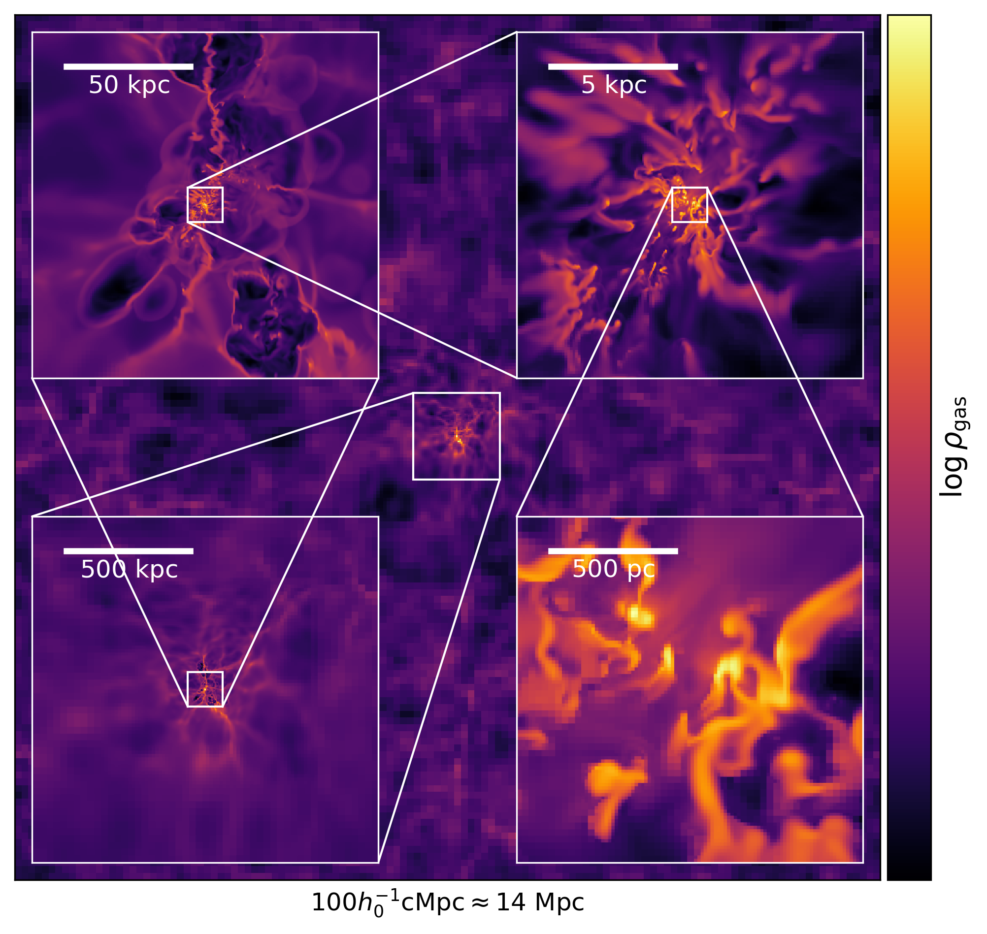
Figure 2: Logarithmic gas density in an $xy$-slice through the most massive galaxy in the fiducial simulation at $z=9$. The main plot shows the entire simulation box with side length $100~{}h_{0}^{-1}{\rm cMpc}\approx 14~{}{\rm Mpc}$. The inset plots show smaller scales, from $\sim 1{\rm Mpc}$ (bottom left) to $\sim 100~{}{\rm kpc}$ (top right) to $\sim 10~{}{\rm kpc}$ (top left) to $1~{}{\rm kpc}$ (bottom right). The range of the density colorbar is adjusted in each inset plot to maximize contrast. At the largest scales, we identify the high resolution zoom region embedded in a cosmological box. At a scale $\sim 100~{}{\rm kpc}$, we identify streams accreting onto the galaxy. Zooming in further, we see the central galaxy and the individual star-forming clumps within. Movies of the simulations are available on YouTube.

Applying this algorithm to each snapshot, we can track the most massive galaxy as it moves through the simulation box. There is no guarantee that the most massive halo at $z>9$ is the progenitor of the most massive halo at $z=9$, so we visually inspect the density field and switch haloes when necessary to enforce continuity. We fit a cubic polynomial to each spatial coordinate of the galaxy center to create a frame which smoothly follows the galaxy. We use this frame to generate movies of our simulations available on YouTube.

3.2 Galaxy structure

In the second and third columns of Figure 3, we show face-on and edge-on projections of the logarithmic gas and star surface densities in a box of side length $2~{}{\rm kpc}$. The procedure for computing the direction of net angular momentum is described in Appendix C. We overlay the in-plane velocity fields as arrows.

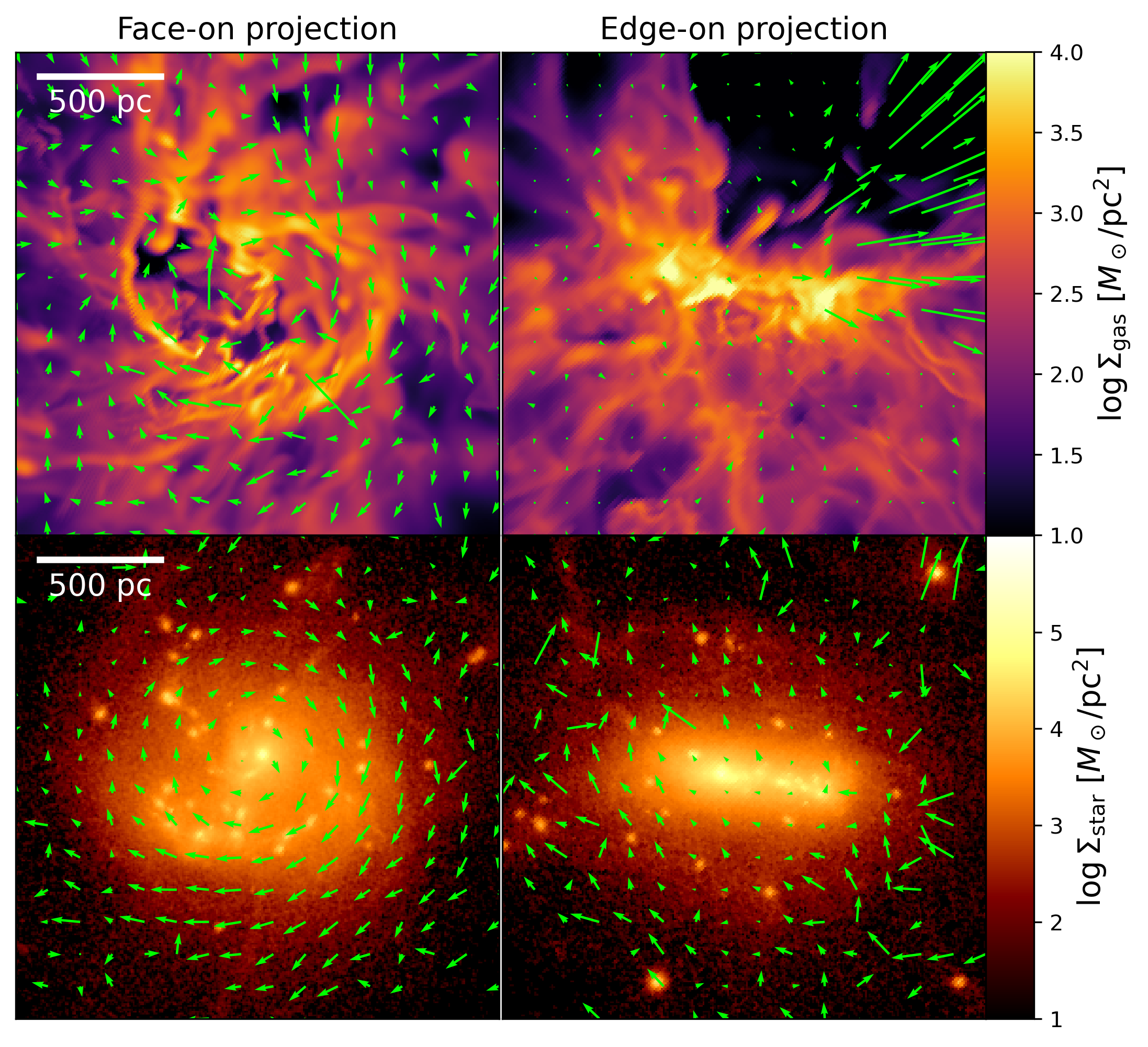
Figure 3: Logarithmic gas (top row) and star (bottom row) surface densities in a box of sidelength $2~{}{\rm kpc}$ around the galaxy center in the fiducial simulation at $z=9$ projected face-on (left column) and edge-on (right column). In each panel, we overlay the in-plane gas (resp. star) velocity field in green, averaged over the projection direction and weighted by gas (resp. star) mass. The galaxy mass is concentrated around a single plane with a rotational velocity field, suggesting a disc structure. The gas and star mass is organized into dense clumps of size $\sim 100~{}{\rm pc}$, although the clump size may be limited by our effective resolution $\simeq 10~{}{\rm pc}$.

The galaxy mass is concentrated around a single plane with a rotational velocity field, suggesting a disc structure. The disciness of the galaxy can be quantified by the scale height $H/R$ and the ratio of the rotational velocity to the radial velocity dispersion $v_{\rm rot}/\sigma_{r}$. The calculation of these metrics is described in Appendix C.

In a rotationally-supported thin disc, we expect $H/R\ll 1$ and $v_{\rm rot}/\sigma_{r}\gg 1$. For gas with temperature $T\leq 10^{4}~{}{\rm K}$, we find a disc height $\approx 326~{}{\rm pc}$ and disc radius $\approx 696~{}{\rm pc}$, giving a scale height $(H/R)_{\rm gas}\approx 0.468$. In addition, we find $v_{\rm rot}/\sigma_{r}\gg 1\approx 2.16$. For stars, we find a disc height $\approx 115~{}{\rm pc}$ and a disc radius $\approx 431~{}{\rm pc}$, giving a scale height $(H/R)_{\rm star}\approx 0.266$. In addition, we find $v_{\rm rot}/\sigma_{r}\approx 0.919$.

These numbers indicate that our galaxy is a thick, rotationally-supported gas disc surrounding a smaller stellar disc. The gas scale height calculation for the disc may be artificially inflated by accretion of cold gas. At lower redshift, MDGs may start to resemble massive star-forming galaxies at cosmic noon, which show disc structures in observation (Förster Schreiber et al., 2006; Genzel et al., 2006, 2008) and simulation (Danovich et al., 2015).

The gas and star mass is organized into dense clumps of size $\sim 100~{}{\rm pc}$, although the clump size may be limited by our effective resolution $\simeq 10~{}{\rm pc}$. Nonetheless, high-redshift disc galaxies show similar structures in observation (Elmegreen et al., 2007; Guo et al., 2012, 2018; Soto et al., 2017) and simulation (Noguchi, 1998; Inoue et al., 2016; Mandelker et al., 2017; Mandelker et al., 2024), strengthening the analogy. The recent simulation work of (Nakazato et al., 2024) find that similar clump structures at high redshifts $z\gtrsim 5$ might be detectable by JWST due to their brightness in rest-frame optical emission lines.

At the locations of these clumps, the face-on gas surface density reaches $\Sigma_{\rm gas}\sim 10^{4}~{}M_{\odot}/{\rm pc^{2}}$ and the Hydrogen number density reaches $n_{\rm H}\sim 3\times 10^{3}~{}{\rm cm^{-3}}$. This represents a much denser environment than Milky-Way-like galaxies with face-on gas surface densities $\Sigma_{\rm gas}\sim 10-100~{}M_{\odot}/{\rm pc^{2}}$ and CNM Hydrogen number densities $n_{\rm H}\sim 10-100~{}{\rm cm^{-3}}$.

3.3 Gas lifecycle

The lifecycle of gas in our simulated galaxies can be understood in temperature-density phase space. In Figure 4, we show the distribution of gas mass in temperature-density phase space for noFbk, SNeOnly, lowPhot, medPhot, and highPhot at $z=9$. Note that the temperature is divided by $\mu$, the mean molecular weight.

We identify multiple ISM gas phases, including the hot ionized medium (HIM; $n_{\rm H}\lesssim 10~{}{\rm cm^{-3}}$ and $T\gtrsim 10^{4}~{}{\rm K}$), the warm neutral medium (WNM; $n_{\rm H}\lesssim 10~{}{\rm cm^{-3}}$ and $T\sim 10^{4}~{}{\rm K}$), the cold neutral medium (CNM; $n_{\rm H}\gtrsim 10~{}{\rm cm^{-3}}$ and $T\lesssim 10^{4}~{}{\rm K}$), and photoionized gas ($n_{\rm H}\gtrsim 10~{}{\rm cm^{-3}}$ and $T\sim 10^{4}~{}{\rm K}$). We remind the reader that the ionization state of the gas only enters into our simulations through the prescribed cooling function.

The black contours in Figure 4 outline the smallest phase space area that contains 75% of star formation events over the course of the simulation. Stars typically form at high densities $\sim 3\times 10^{3}~{}{\rm cm^{-3}}$ and low temperatures $\sim 300~{}{\rm K}$. The star-forming regions of phase space contain very little gas because any gas that enters this region is quickly removed by star formation or feedback. The red contours outline the smallest phase space area that contains 75% of SN events occur. The SN events are distributed between the CNM, photoionized gas, and the HIM.

Whether gas evolves horizontally or vertically in phase space is a question of timescales. When the cooling timescale is longer than the freefall time, gas collapses, moving horizontally to higher densities. When the freefall time is longer than the cooling timescale, gas cools, moving vertically to lower temperatures. At a fixed temperature and metallicity, we have $\tau_{\rm cool}\propto\rho^{-1}$ and $\tau_{\rm ff}\propto\rho^{-1/2}$, so collapsing gas will eventually reach a density where cooling dominates.

The lower right panel of Figure 4 is schematic diagram illustrating the progression of gas through the phase space in steps: (i) gas from streams collapses as it accretes onto the galaxy, joining the HIM; (ii) the gas cools to the Hydrogen ionization temperature $\sim 10^{4}~{}{\rm K}$, where it becomes neutral and joins the WNM; (iii) the neutral gas cools less efficiently than the ionized gas, so it collapses while maintaining approximately the same temperature; (iv) once the density becomes sufficiently high, cooling becomes efficient and the gas joins the CNM; (v) eventually, stars begin to form and photoionization feedback generates photoionized gas at $\sim 10^{4}~{}{\rm K}$; (vi) the gas continues to collapse until it once again becomes cold and dense enough to form stars; (vii) SN explosions can recycle gas in any of the previous stages back into the WNM or HIM.

We can build up this picture by starting with our most simple simulation noFbk. In this simulation, gas accretes, cools, and collapses following steps (i)-(iii). However, without SNe to enrich the gas with metals, the gas is pristine and must reach high densities $\sim 300~{}{\rm cm^{-3}}$ before it can cool below $\sim 10^{4}~{}{\rm K}$. At this point, the gas is so dense that it only needs to cool to $\sim 1000~{}{\rm K}$ before stars form efficiently. This also describes the formation of the first generation of stars in simulations that include SNe.

The most striking difference between noFbk and SNeOnly is the presence of gas at extreme temperatures $\gtrsim 10^{7}~{}{\rm K}$. This gas must be produced by SNe exploding in diffuse gas. This can occur when a young star cluster particle diffuses into a diffuse region over its lifetime, or when the local gas conditions around a star cluster particle are modified by early feedback or other SNe.

Metal-enriched gas starts to cool below $\sim 10^{4}~{}{\rm K}$ at densities $\gtrsim 10~{}{\rm cm^{-3}}$. The cooling and collapsing gas forms a diagonal band in phase space. Eventually, gas reaches the CMB temperature $\simeq 27.25~{}{\rm K}$ and becomes dense enough to form stars. The metal enriched gas ends up forming stars at lower densities than pristine gas.

In simulations with photoionization feedback, star formation immediately generates photoionized gas. After a few timesteps, the temperature of the gas is set by a balance between the thermal energy injected by photoionization and the thermal energy removed by cooling. As gas collapses, the cooling rate increases and gas is able to reach lower temperatures, producing a second diagonal band in phase space. In highPhot where photoionization is more efficient, stars form at higher temperatures than lowPhot, where photoionization is less efficient.

We do not resolve the multi-phase nature of the ISM on small scales, so the high temperatures of star formation in the simulations with photoionization does not mean that stars form out of high-temperature gas. Instead, the temperature of star formation reflects the filling factor of photoionized gas near star formation sites on unresolved scales.

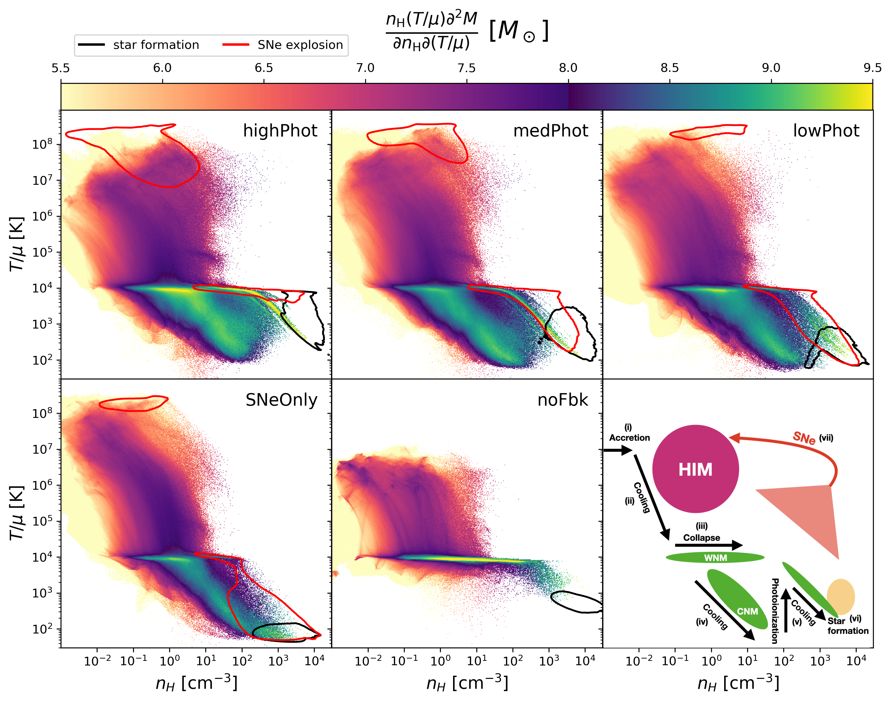
Figure 4: Two-dimensional histograms of the density and temperature in a box of sidelength $5~{}{\rm kpc}$ around the most massive galaxy at $z=9$ weighted by gas mass for highPhot, medPhot, lowPhot, SNeOnly, and noFbk. The temperature is normalized by $\mu$, the mean molecular weight. The color bar represents the phase space density i.e. the mass per bin in logarithmic density and temperature. Hotter and more diffuse gas has relatively less mass per bin and is represented by purple colors. Colder and more dense gas has relatively more mass per bin and is represented by green colors. We overplot contours outlining the smallest phase space areas containing $75\%$ of star formation events weighted by stellar mass (black) and $75\%$ of SN events (red). In the bottom right panel, we show a schematic diagram of the gas evolution, explained in Section 3.4.

3.4 Local gas properties

In Figures 5 and 6, we show the mass-weighted and volume-weighted distributions respectively of gas density, temperature, turbulent velocity dispersion, and metallicity for the early feedback and turbulence forcing series. We plot turbulent velocity dispersion rather than turbulent Mach number to isolate the differences in turbulence between simulations from the temperature-dependence $\mathcal{M}_{\rm turb}\propto T^{-0.5}$ at a constant TKE.

Compared to the lower-redshift Universe, the gas has higher densities, higher turbulent velocity dispersions, and lower metallicities. The mass-weighted density and temperature distributions in the early feedback series are consistent with the two-dimensional histograms in Figure 4.

HII regions created by photoionization feedback produce a sharp peak in the temperature distribution at $\sim 10^{4}~{}{\rm K}$. The density distribution does not change significantly across the early feedback series, suggesting that the thermal pressure from photoionization feedback is insufficient to halt the collapse of the star-forming clouds. This is expected, because for high mass star-forming clouds $M_{\rm cl}\gtrsim 10^{6}~{}M_{\odot}$, the sound speed $c_{\rm s}\sim 10~{}{\rm km/s}$ in photoionized gas is less than the escape speed of the cloud (e.g. Krumholz & Matzner, 2009).

The volume-weighted distributions tell a similar story. In this case, the peak in the temperature distribution at $T\sim 10^{4}~{}{\rm K}$ represents the volume of WNM rather photoionized gas, whose volume fraction is generally smaller. As photoionization feedback becomes more efficient, volume moves from ultra-diffuse HIM gas $\lesssim 10^{-2}~{}{\rm cm^{-3}}$ to WNM gas $\sim 10^{-1}~{}{\rm cm^{-3}}$.

Solenoidal forcing decreases the local SFE for the same gas conditions and TKE. Therefore, gas must reach higher densities to form stars efficiently, resulting in more gas mass at high densities $\gtrsim 10^{3}~{}{\rm cm^{-3}}$.

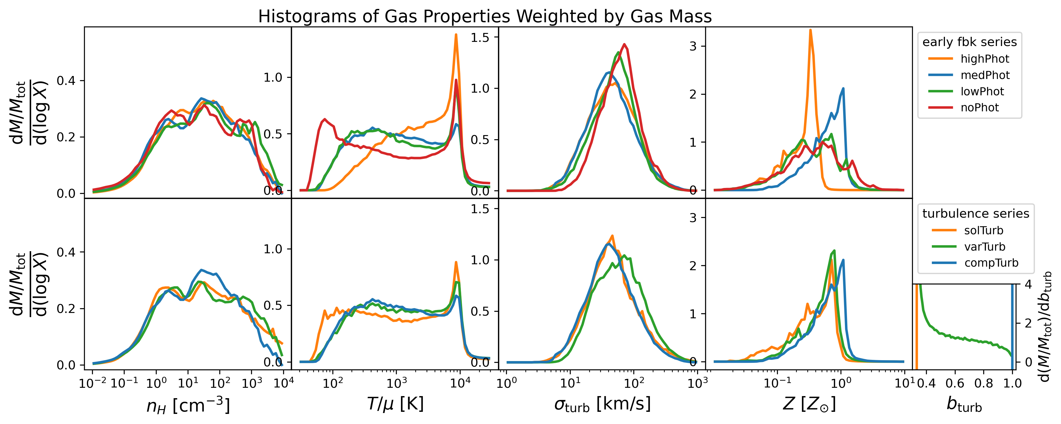
Figure 5: Histograms of the hydrogen number density (first column), modified temperature (second column), turbulent velocity dispersion (third column), and metallicity (fourth column) in a box of sidelength $5~{}{\rm kpc}$ around the most massive galaxy at $z=9$ in the early feedback series (top row) and turbulence forcing series (bottom row), weighted by gas mass. Each simulation is shown in a different color, with the fiducial simulation in blue. An additional histogram of the turbulence forcing parameter is included for the turbulence forcing simulation.

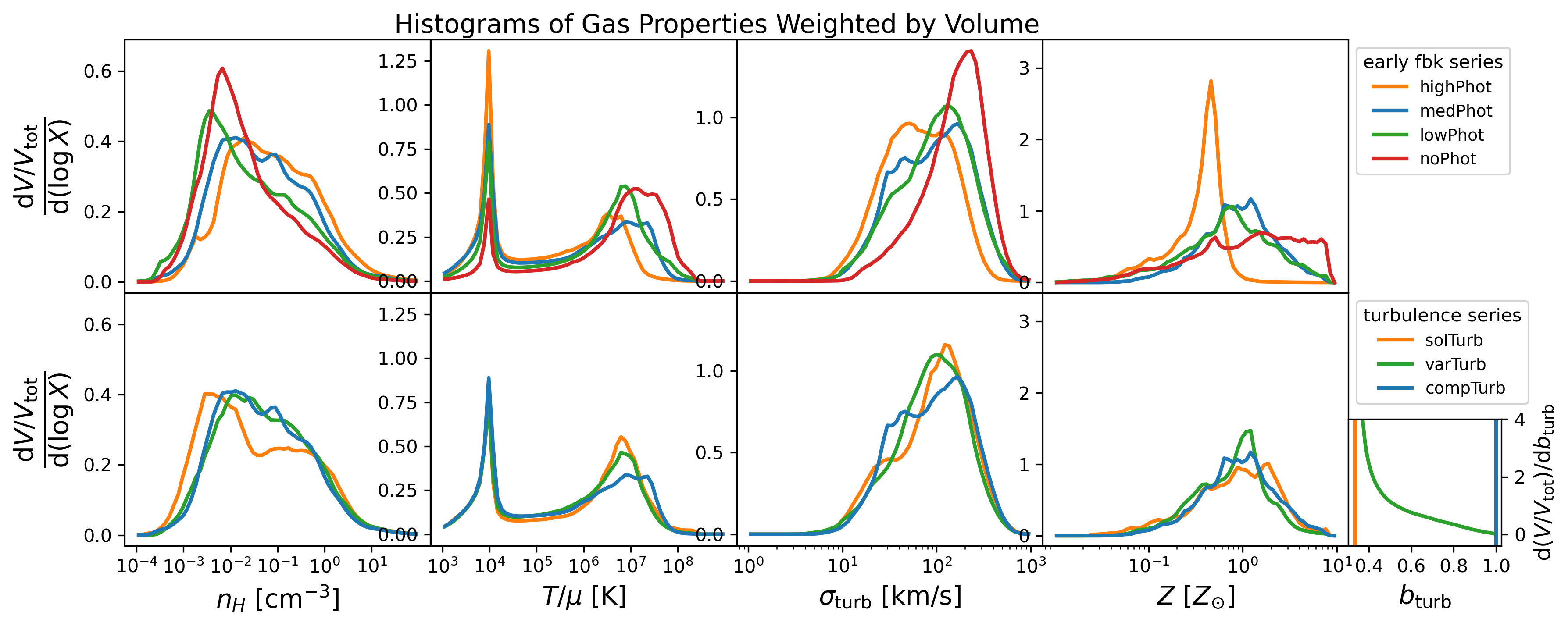
Figure 6: Histograms of the hydrogen number density (first column), modified temperature (second column), turbulent velocity dispersion (third column), and metallicity (fourth column) in a box of sidelength $5~{}{\rm kpc}$ around the most massive galaxy at $z=9$ in the early feedback series (top row) and turbulence forcing series (bottom row), weighted by volume. Each simulation is shown in a different color, with the fiducial simulation in blue. An additional histogram of the turbulence forcing parameter is included for the turbulence forcing simulation.

In Figure 7, we show the distributions of gas density, temperature, turbulent velocity dispersion, and metallicity in star-forming cells for the early feedback and turbulence forcing series. In the early feedback series, photoionization feedback forces stars to form at higher temperatures. Therefore, the gas must reach higher densities and lower turbulent velocity dispersions for star formation to become efficient. This explains the trends of increasing density and decreasing turbulent velocity dispersion with increasing photoionization feedback efficiency.

A similar analysis applies to the turbulence forcing series. In the solenoidal forcing limit, the SFE is lower for the same gas conditions, so gas must reach higher densities, lower temperatures, and lower turbulent velocity dispersions for star formation to become efficient. This explains the trends of increasing star-formation density and decreasing star-formation temperature with increasingly solenoidal turbulence forcing.

However, the trend in the turbulent velocity dispersion seems to go the wrong way, increasing as the turbulence forcing becomes more solenoidal. The reason is that regions of high density, low temperature, and high turbulence are spatially coincident (App. F). In solTurb, stars are forced to form in high density and low temperature regions, which also forces them to form in high turbulence regions, even though turbulence generally decreases the local SFE.

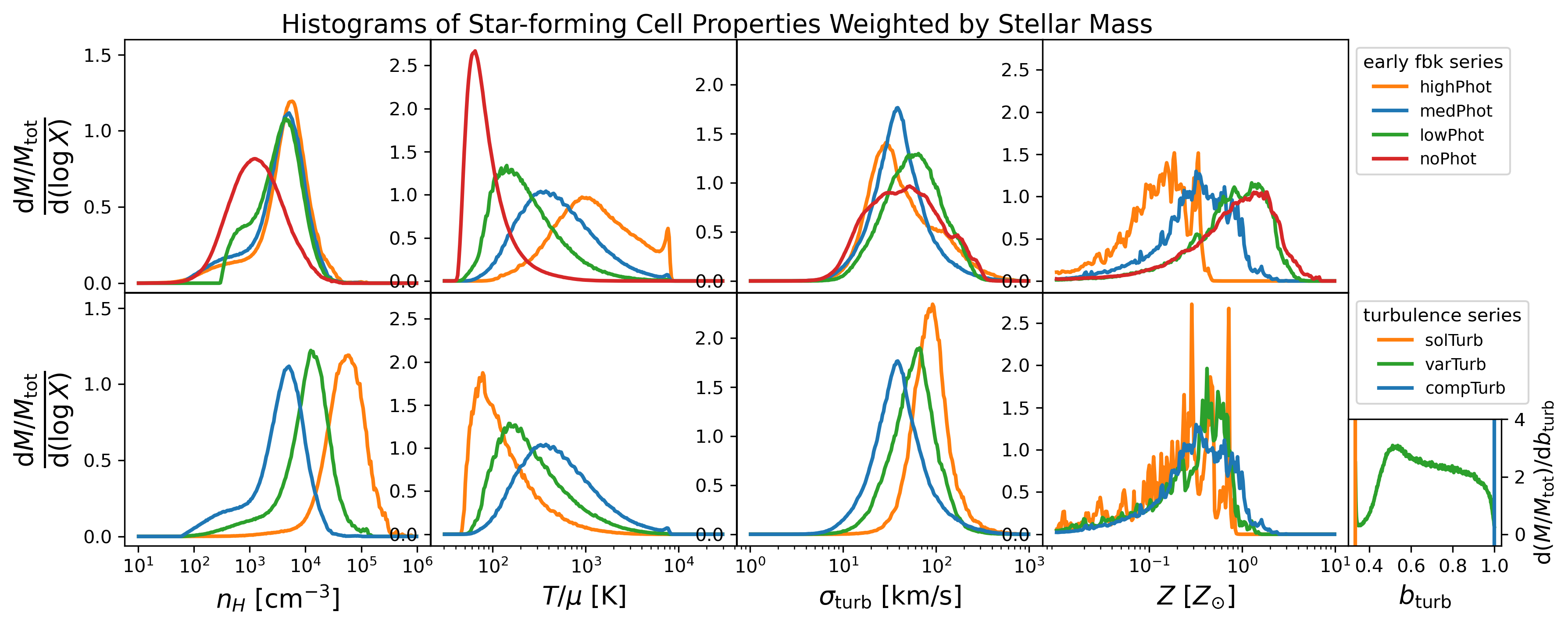
Figure 7: Histograms of the hydrogen number density (first column), modified temperature (second column), turbulent velocity dispersion (third column), and metallicity (fourth column) of star-forming cells in the early feedback series (top row) and turbulence forcing series (bottom row), weighted by stellar mass. Each simulation is shown in a different color, with the fiducial simulation in blue. The inset plot shows a histogram of the turbulence forcing parameter for the turbulence forcing series. An additional histogram of the turbulence forcing parameter is included for the turbulence forcing simulation.

In Figure 8, we show the distributions of gas density, temperature, turbulent velocity dispersion, and metallicity in cells where a SN event occurs for the early feedback and turbulence forcing series. The distribution of gas conditions near SNe is multi-modal, reflecting the multi-phase nature of the ISM. As photoionization feedback becomes more efficient, more SNe occur in photoionized gas and HIM rather than CNM. This effect can also be seen in Figure 4, where the portion of the red contour in photoionized gas and HIM expands as photoionization feedback becomes more efficient. SNe occur in more dense environments as turbulence forcing becomes more solenoidal, following the trend in the density of star-forming cells.

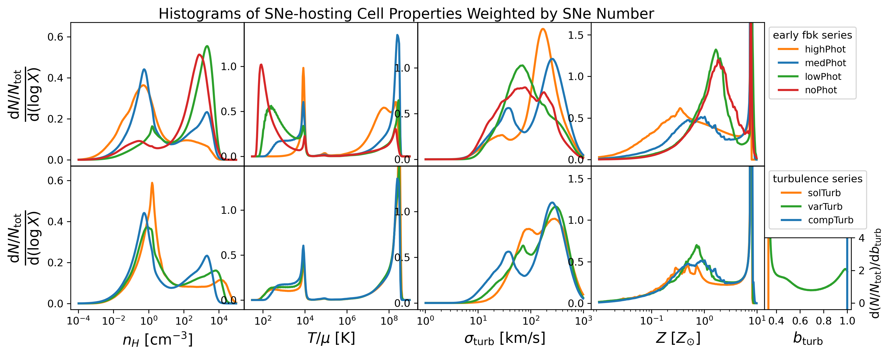
Figure 8: Histograms of the hydrogen number density (first column), modified temperature (second column), turbulent velocity dispersion (third column), and metallicity (fourth column) of cells with SN events in the early feedback series (top row) and turbulence forcing series (bottom row), weighted by SN number. Each simulation is shown in a different color, with the fiducial simulation in blue. An additional histogram of the turbulence forcing parameter is included for the turbulence forcing simulation.

In the SN feedback series, we vary the SN delay time $\tau_{\rm start}$. We find that the summary statistics and gas property distributions (not shown in figures) are almost identical for all simulations in the series. This suggests that the SN delay time is not important for star formation, even in the extreme case of instSNe where SNe can occur immediately after star formation.

Our finding contradicts the prediction of the FFB model (Dekel et al., 2023) that the SN delay time provides a crucial window of opportunity for efficient star formation. However, our ability to test the FFB model is limited by our resolution $\Delta x_{\rm min}\simeq 10~{}{\rm pc}$. We cannot fully resolve the parsec-scale dynamics which control star-forming clouds, especially in dense regions where the SN cooling radius is unresolved (Sec. 4.7).

3.5 Star formation histories

At a high level, we describe the SFH using summary statistics in Table 1, including the total stellar mass $M_{*}$ in the galaxy at $z=9$, the average SFR over the last $50~{}{\rm Myr}$ at $z=9$ ${\rm SFR}_{50}$, the integrated SFE $\epsilon_{\rm int}$, the median local SFE ${\rm med}(\epsilon_{\rm ff})$, and the outflow efficiency $\eta$. The calculation of these summary statistics is described in Appendix D. Nearly all our simulations produce significant stellar populations ($M_{*}\gtrsim 10^{9}~{}M_{\odot}$) with high SFRs ($\dot{M}_{*}\gtrsim 100~{}M_{\odot}/{\rm yr}$) and high SFEs ($\epsilon_{\rm ff},\epsilon_{\rm int}\gtrsim 10\%$), supporting the notion that star formation is intrinsically efficient at Cosmic Dawn.

Throughout this paper, we use 3 different measurements of SFE. The local SFE $\epsilon_{\rm ff}$ is the fraction of gas within a single cell that is converted into stars within one local freefall time. The global SFE $\epsilon_{\rm glob}=\dot{M}_{*}/f_{\rm b}\dot{M}_{\rm acc}$ is the ratio of the SFR in the galaxy to the gas accretion rate. The integrated SFE $\epsilon_{\rm int}=M_{*}/f_{\rm b}M_{\rm halo}$ is the ratio of the stellar mass to the total gas mass accreted onto the galaxy over its lifetime. The distinction between these SFEs highlights that any measure of SFE is defined on a particular spatial and temporal scale. Measurements of the SFE on multiple scales are necessary ingredients of a holistic picture of star formation.

Figures 9 and 10 visually represent the integrated and local SFEs respectively. In Figure 9, we show the stellar mass as a function of time, which is proportional to the integrated SFE. In Figure 10, we show the distribution of local SFEs in star formation events.

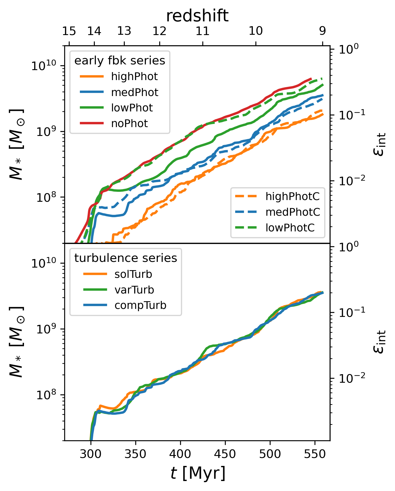
Figure 9: Stellar mass as a function of time for the early feedback series (top panel) and turbulence forcing series (bottom panel). The integrated SFE defined relative to the halo mass at $z=9$ is shown on a secondary $y$-axis in both panels. Within each series, each simulation is shown in a different color, with the fiducial simulation in blue. Dashed lines in the upper panel indicate constant SFE simulations. The stellar mass increases almost exponentially with time, following the expected accretion rate onto a dark matter halo in the early Universe.

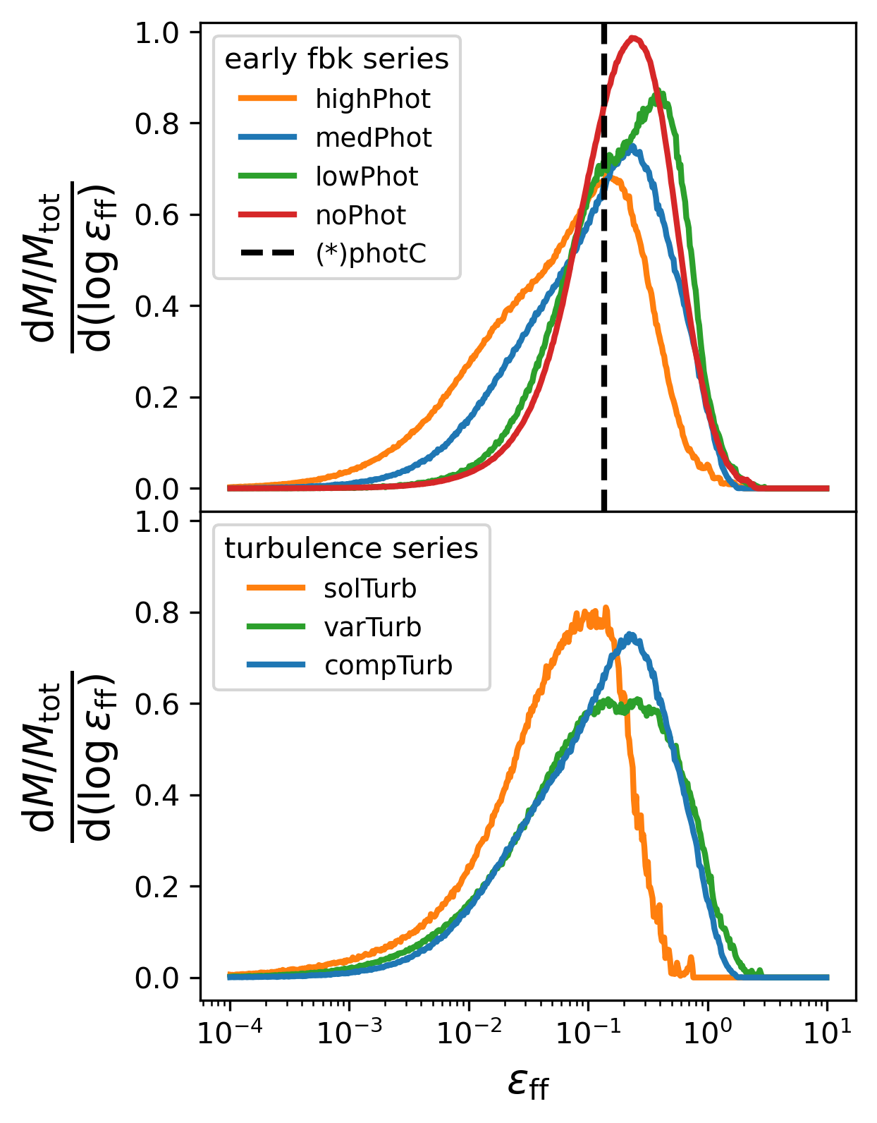
Figure 10: A histogram of local SFE weighted by stellar mass for the early feedback series (top panel) and the turbulence forcing series (bottom panel). Within each series, each simulation is shown in a different color, with the fiducial simulation in blue. The dashed line in the upper panel indicates the local SFE of the constant local SFE simulations. In all simulations, the local SFE ranges from $\sim 1\%$ to $\sim 100\%$, reflecting the large range of gas conditions in which stars can form.

The relative factors between the stellar masses of different simulations remain approximately constant throughout time, implying that the differences between simulations are not redshift dependent for $z\geq 9$. This lends credence to our approach of analyzing a single snapshot in time at $z=9$.

The stellar mass, and therefore also the mean SFR, increases almost exponentially with time, following the expected accretion rate onto a dark matter halo in the early Universe (Sec. 4.1). In all simulations, the local SFE ranges from $\sim 1\%$ to $\sim 100\%$, reflecting the large range of gas conditions in which stars can form (Fig. 7).

Comparing photOnly to noFbk, we isolate the effect of photoionization feedback. Both simulations have similar integrated and local SFEs, suggesting that by itself photoionization feedback is ineffective at suppressing star formation. Alternatively, comparing SNeOnly to noFbk, we isolate the effect of SN feedback. SNeOnly has a lower integrated SFE but a similar local SFE, suggesting that SN feedback suppresses star formation without changing the local gas conditions at star formation sites.

In yesFbk, both feedback mechanisms operate simultaneously. yesFbk has the lowest integrated and local SFE in the feedback series. The low integrated SFE is surprising because it suggests that photoionization is effective, but only in tandem with SN feedback. The low local SFE is also surprising, because it suggests that when both feedback mechanisms work together, they alter the local gas conditions, even though this effect is not seen for either mechanism in isolation.

In the early feedback series, the integrated and local SFEs change by a similar factor between simulations. For example, from medPhot to highPhot, both efficiencies decrease by a factor of 2. Therefore, it is tempting to conclude that the integrated SFE is proportional to the local SFE, which is consistent with a picture where star formation is not regulated by feedback. However, our other simulations provide evidence to the contrary.

First, the constant efficiency simulations all have a fixed local SFE, but they show the same trend in integrated SFE as the MFF simulations. Second, in the turbulence forcing series, the local SFE decreases by a factor of 3 as turbulence forcing becomes more solenoidal. The trend in integrated SFE goes in the same direction, but by a much smaller factor. These results do not rule out a correlation between local and integrated SFE, but they suggest that the local SFE is not the main driver for the trends we see.

The trends in outflow efficiency suggest an alternative explanation. SNe can regulate star formation by launching outflows which remove gas from the galaxy. When there are no SNe (noFbk and photOnly), the galaxy is not able to launch outflows $\eta\approx 0$. When there are SNe, we see a small outflow efficiency $\eta\simeq 0.5$.

As photoionization feedback becomes more efficient, the outflow efficiency increases, reaching $\eta\simeq 10$ in highPhot. This suggests that photoionization feedback suppresses star formation by enhancing the ability of SN explosions to drive outflows. This interpretation is supported by the local gas properties, which show that photoionization feedback is associated with (i) an increase in the volume fraction of the WNM (Fig. 6) and (ii) more SN explosions in photoionized gas and HIM rather than CNM (Fig. 8).

When SNe occur in more diffuse gas, more of their energy makes it into the ISM rather than being absorbed locally and radiated away. Once in the ISM, this energy can suppress star formation by disrupting star-forming clouds and launching outflows.

These data do not directly prove our interpretation because they only establish correlation rather than causation. However, previous works have come to similar conclusions regarding the interplay of photoionization and SN feedback. For example, Rosdahl et al. (2015) find that photo-heating smooths the density field in their disc galaxies, enhancing the effectiveness of SN feedback (their Fig. 9).

3.6 Star formation variability

In the first row of Figure 11, we plot the SFR as a function of time. The calculation of the SFR is described in Appendix D. The SFR fluctuates on multiple timescales, from small bursts lasting only a few ${\rm Myr}$ to large bursts lasting 10s of ${\rm Myr}$. Because the mean SFR increases rapidly as a function of time, measurements of the SFR on long timescales may under-represent the instantaneous SFR (Sec. 4.9.1).

After major bursts, the SFR temporarily decreases, possibly because the bursts consume dense gas available to form stars. The movies associated with this paper reveal that the major bursts in the SFR coincide with significant merger events, although analyzing the role of mergers in detail is beyond the scope of this paper.

We quantify the variability of the SFR using the power spectral density (PSD) in the time domain. To compute the PSD, we follow a similar procedure to Iyer et al. (2020). We start with the SFR in time bins of width $\Delta t=0.1~{}{\rm Myr}$, which gives a reasonable balance between shot noise and time resolution. We work with the logarithm of the SFR so that fluctuations in the SFR are measured relative to the mean rather than on an absolute scale. If we worked with the raw SFR, then the variability calculated at early times would be smaller than the variability calculated at late times just because the mean SFR is lower.

We can remove the exponential trend in the mean SFR with a linear detrending of the logarithmic SFR. We limit our analysis to times $\geq 350~{}{\rm Myr}$, when all simulations have a nonzero SFR such that the logarithm is well-defined. The second row of Figure 11 shows the residuals of the linear detrending.

Finally, we apply Welch’s method (Welch, 1967) as implemented by scipy.signal.welch. In this method, the data are divided into overlapping segments. We choose segments of 256 bins which 50% overlap on each side with their neighbors. We compute a modified periodogram for each segment and then average the periodograms. We use the Hann window function in the computation of each periodogram to reduce edge effects.

In the third row of Figure 11, we plot the PSD of the SFR in the third row of Figure 11, inverting the $x$-axis to plot against fluctuations timescale rather than frequency. The PSD has three regimes. On short timescales, the PSD is flat and represents uncorrelated noise. On intermediate timescales, the PSD roughly follows a power law $\mathcal{P}\propto(\Delta t)^{2}$. This red noise is characteristic of the damped random walk expected from a stochastic Orstein-Uhlenbeck process (Caplar & Tacchella, 2019).

The transition between these two regimes occurs on a timescale $\sim 1~{}{\rm Myr}$, which can be interpreted as our star formation timescale i.e. the free-fall time in a star forming cloud. On shorter timescales, it is impossible for one star formation event to be correlated with another. A freefall time $\sim 1~{}{\rm Myr}$ is associated with a density $\sim 3\times 10^{3}~{}{\rm cm^{-3}}$, which we can use as an estimate for the typical density of star formation.

On longer timescales, the PSD becomes flat again. The transition between these two regimes occurs on a timescale $\sim 10~{}{\rm Myr}$, which can be interpreted as the lifetime of star forming clouds in our simulation (Tacchella et al., 2020). Due to the 550 Myr duration of our simulations, we cannot compute the PSDs on longer timescales using Welch’s method. However, one might expect the PSDs to regain a positive slope at even longer timescales due to correlations caused by galaxy mergers, outflow recycling, and other processes affecting the gas reservoir (Tacchella et al., 2020).

Figure 11: SFR (first row), logarithmic SFR residuals (second row), and the PSD of the SFR (third row) for the early feedback series (left column) and the turbulence forcing series (right column). Within each series, each simulation is shown in a different color, with the fiducial simulation in blue. The transition from white noise to red noise occurs on the star formation timescale $\sim 1~{}{\rm Myr}$. The transition from red noise back to white noise occurs on timescale representing the lifetime of star forming clouds $\sim 10~{}{\rm Myr}$.

Our star formation histories show some agreement with the FFB model (Dekel et al., 2023). The timescale of 10s of ${\rm Myr}$ is similar to the timescale predicted for generations of FFBs (Li et al., 2024). In addition, the highest star formation rates are achieved during a time window of $\sim 80~{}{\rm Myr}$ between $z=10$ and $z=9$, similar to the halo-crossing timescale predicted by Dekel et al. (2023) over which FFBs are active. However, a longer simulation is required to see if rapid star formation is suppressed by feedback from earlier generations of star clusters.

3.7 Variable turbulence forcing parameter

In varTurb, we determine the turbulence forcing parameter from the local velocity field using Equation 15. varTurb behaves almost like a simulation with constant forcing parameter in between the solenoidal and compressive forcing limits. In Figure 7, the density, temperature, and turbulent velocity dispersion of star-forming cells for varTurb is somewhere in between the distributions for solTurb and compTurb.

However, in some metrics, varTurb deviates from this behavior. The median local SFE in varTurb is nearly the same as compTurb and the turbulent velocity dispersion of the gas is higher in varTurb than in solTurb or compTurb.

These effects can be explained because stars preferentially form in compressively forced regions, which have a higher local SFE for the same gas conditions and TKE. This is apparent in the forcing parameter distribution for star-forming cells (Fig. 7), which is shifted more towards the compressive end than the forcing parameter distribution for the gas (Fig. 5). Because a disproportionate number of stars form in compressively forced regions, the local SFE distributions are similar between varTurb and compTurb. Our fiducial model, which assumes the compressively forced limit, is therefore a reasonable approximation for model varTurb, where the forcing parameter is determined more self-consistently.

In Appendix F, we show the turbulence forcing parameter in an $xy$-slice through the galaxy in the fiducial simulation at $z=9$. Close to the galaxy, most of the volume is dominated by solenoidal forcing, but there are small pockets of compressive forcing. The turbulence forcing parameter distribution of SN-hosting cells (Fig. 8) has a peak at the compressive forcing limit $b_{\rm turb}=1.0$, hinting that these pockets may be formed by SN explosions.

We leave a more rigorous analysis of self-consistent turbulence forcing to future work which simulations the forcing parameter more carefully. Mandelker et al. (2024) describe a more rigorous approach to implement a self-consistent forcing parameter which involves decomposing the shear tensor into three components representing compression, solid body rotation and shear flow. Their method will be described in an upcoming paper (Ginzburg et. al., in prep.).

4 Discussion

In this section, we interpret our results with toy models, compare to similar works, and discuss observational implications. First, we show that when the gas depletion time is sufficiently short, star formation and gas metallicity are regulated by ejective stellar feedback (Sec. 4.1 and 4.2). Then, we show that the previous arguments are predicated on the high local SFE in MDGs (Sec. 4.3). Next, we describe the relationship between turbulence and star formation (Sec. 4.4). Then, we discuss the role of early feedback processes not included in our models (Sec. 4.5). Next, we discuss the limitations of our star formation recipe (Sec. 4.6), SN feedback recipe (Sec. 4.7), and other aspects of our modeling (Sec. 4.8). Finally, we discuss the observational implications of our results (Sec. 4.9).

4.1 Self-regulation of global SFE

We can use a simple one-zone model to explain the global SFE in our simulations and the exponential growth of the stellar mass, inspired by the “bathtub” toy model of Dekel & Mandelker (2014) and similar models from earlier works (e.g. Tinsley, 1968). The gas mass $M_{\rm gas}$ in a galaxy is depleted by star formation and outflows. Simultaneously, the gas mass is augmented by accretion and SN explosions. These processes can be described by a differential equation:

$$\begin{split}\dot{M}_{\rm gas}=\ &f_{\rm b}\dot{M}_{\rm acc}-\dot{M}_{*}+\dot{M}_{\rm SNe}-\dot{M}_{\rm out}\\ =\ &f_{\rm b}\dot{M}_{\rm acc}-(1-\chi+\eta)\dot{M}_{*}\end{split}$$ (36)

where $\chi$ is the mass fraction of massive stars and $\eta=\dot{M}_{\rm out}/\dot{M}_{*}$ is the outflow efficiency. The model can account for the recycling of gas by adding negative contributions to $\eta$.

The outflow efficiency characterizes the strength of ejective feedback, the component of stellar feedback that removes gas from the galaxy. Preventative feedback, the component of stellar feedback which does not remove gas from the galaxy, can still suppress star formation by moving gas out of the star-forming state, but its effect on the global SFE is more subtle (App. H).

If $\dot{M}_{*}\propto M_{\rm gas}$ and $\dot{M}_{\rm acc}$ is constant, then Equation 36 asymptotically approaches a steady state solution where $\dot{M}_{\rm gas}=0$ (Dekel & Mandelker, 2014). In practice, $\dot{M}_{\rm acc}$ changes as a function of time. However, if the gas depletion time $\tau_{\rm dep}=M_{\rm gas}/\dot{M}_{*}$ is short compared to the timescale on which the accretion rate changes $\tau_{\rm acc}=\dot{M}_{\rm acc}/\ddot{M}_{\rm acc}$, then we can treat $\dot{M}_{\rm acc}$ as constant. We estimate values for $\tau_{\rm dep}$ and $\tau_{\rm acc}$ relevant to our simulations in Sec. 4.3.

Setting $\dot{M}_{\rm gas}=0$ in Equation 36, we find

$$\dot{M}_{*}=\frac{f_{\rm b}\dot{M}_{\rm acc}}{1-\chi+\eta}$$ (37)

Dividing by the accretion rate to get the global SFE, we find

$$\epsilon_{\rm glob}=\frac{1}{1-\chi+\eta}$$ (38)

The global SFE is independent of the local SFE and decreases with stronger ejective feedback. We call this behavior self-regulation, because the SFR is regulated by stellar feedback. Self-regulation is consistent with the trend in decreasing integrated SFE with increasing outflow efficiency in our simulations (Sec. 3.5).

Equation 37 also demonstrates that the SFR is proportional to the gas accretion rate onto the galaxy. At Cosmic Dawn, the Universe is well-approximated by an Einstein-deSitter (EdS) cosmology. The specific accretion rate onto a halo of mass $M_{\rm halo}$ in an EdS universe is approximately (Dekel et al., 2013)

$$\frac{\dot{M}_{\rm acc}}{M_{\rm halo}}\simeq s\left(\frac{M_{\rm halo}}{10^{12}~{}M_{\odot}}\right)^{\beta}(1+z)^{5/2}$$ (39)

where $\beta$ is the power law exponent of the fluctuation power spectrum and $s$ is the specific accretion rate into a halo of $M_{\rm halo}=10^{12}~{}{\rm M_{\odot}}$ at $z=0$. Dekel et al. (2013) find that values $\beta\simeq 0.14$ and $s\simeq 0.030~{}{\rm Gyr^{-1}}$ are consistent with the Millennium cosmological simulation (Springel et al., 2005).

Ignoring the weak $M_{\rm halo}^{\beta}$ dependence and integrating, we find (Dekel et al., 2013, Eq. 9)

$$M_{\rm halo}\simeq M_{\rm halo,0}e^{-\alpha(z-z_{0})}$$ (40)

where $M_{\rm halo,0}$ is the halo mass at redshift $z_{0}$, $\alpha=(3/2)st_{\rm H,0}$, $t_{\rm H,0}=(2/3)\Omega_{\rm m,0}^{-1/2}H_{0}^{-1}\approx 17.5~{}{\rm Gyr}$ is the age of an EdS universe at redshift $z=0$, and we have used

$$a=(1+z)^{-1}=\left(\frac{t}{t_{\rm H,0}}\right)^{2/3}$$ (41)

This implies that the accretion rate onto a given halo as it grows is (Dekel et al., 2013, Eq. 10)

$$\dot{M}_{\rm acc}(z)\simeq sM_{\rm halo,0}e^{-\alpha(z-z_{0})}(1+z)^{5/2}$$ (42)

At high redshift, the accretion rate is well-described as an exponential function of redshift (see also Correa et al., 2015). Therefore, the exponential growth of stellar mass in our simulated galaxies is simply a reflection of the exponential growth of the halo accretion rate.

4.2 Metal enrichment

Using a similar approach, we can describe the process of metal enrichment. The metal mass in a galaxy is governed by

$$\begin{split}\dot{M}_{\rm metal}=\ &-Z(\dot{M}_{*}+\dot{M}_{\rm out})+y\dot{M}_{\rm SNe}\\ =\ &-[Z(1+\eta)-y\chi]\dot{M}_{*}\end{split}$$ (43)

where $y$ is the SN metal yield and we have assumed that the metal content of the primordial, accreting gas in negligible.

This model assumes that metals produced in SN explosions are rapidly mixed throughout the ISM rather than remaining localized to the SN site. The turbulent environment at Cosmic Dawn facilitates that mixing. Our simulated galaxies have typical velocity dispersions $\sigma_{\rm turb}\simeq 40~{}{\rm km/s}$ and radii $R_{\rm gal}\simeq 1~{}{\rm kpc}$, so the metal mixing time is approximately $\tau_{\rm mix}\sim R_{\rm gal}/\sigma_{\rm turb,1D}\simeq 30~{}{\rm Myr}$, far shorter than the lifetime of the galaxy.

Again assuming a steady state $\dot{M}_{\rm metal}=0$, we find that

$$Z=y\chi/(1+\eta)$$ (44)

In our simulations, we have $y=0.1$ and $\chi=0.2$. If the outflow efficiency is negligible $\eta\approx 0$, then we have $Z\approx 0.02\approx 1~{}Z_{\odot}$, which is similar to the typical gas metallicity in noPhot (Fig. 5).

If, on the other hand, outflows become efficient at removing gas, then the gas metallicity will be reduced accordingly. For example, $1+\eta$ is larger by a factor of 5 in highPhot compared to medPhot, and the typical gas metallicity is reduced by the same factor.

4.3 Condition for self-regulation

Section 4.1, we assume that the depletion timescale is short compared to the accretion timescale, and therefore the gas mass reaches a steady state. To define the condition for steady state more precisely, we apply a bathtub-like model to the star-forming gas mass $M_{\rm sf}$, following the arguments of Semenov et al. (2017) and Semenov et al. (2018).

Star-forming gas is depleted by star formation, stellar feedback, and dynamical processes (e.g. turbulent shear) operating on a timescale $\tau_{\rm dyn}$. Simultaneously, star-forming gas is augmented by cooling and collapse on a timescale $\tau_{\rm cool}$. These processes can be described by a differential equation

$$\dot{M}_{\rm sf}=\frac{1-f_{\rm sf}}{\tau_{\rm cool}}M_{\rm gas}-\frac{f_{\rm sf}}{\tau_{\rm dyn}}M_{\rm gas}-(1+\mu)\dot{M}_{*}$$ (45)

where $f_{\rm sf}=M_{\rm gas}/M_{\rm sf}$ is the star-forming mass fraction and $\mu\dot{M}_{*}$ is the rate at which gas mass is removed from the star-forming state by stellar feedback. $\mu$ characterizes the strength of preventative feedback.

The timescales $\tau_{\rm cool}$, $\tau_{\rm ff}$, and $\tau_{\rm dyn}$ which set the star-forming gas mass are shorter than the accretion timescale, so we can assume a steady state where $\dot{M}_{\rm sf}=0$. Then, we can solve for $f_{\rm sf}$, which yields

$$f_{\rm sf}=\frac{\tau_{\rm ff}}{\epsilon_{\rm ff}}\left[f_{\rm dyn}\frac{\tau_{\rm ff}}{\epsilon_{\rm ff}}+(1+\mu)\tau_{\rm cool}\right]^{-1}$$ (46)

where $f_{\rm dyn}=1+\tau_{\rm cool}/\tau_{\rm dyn}$ is a factor of a few. We have assumed that the SFR is related to the gas mass by the Schmidt Law

$$\dot{M}_{*}=\frac{\epsilon_{\rm ff}}{\tau_{\rm ff}}f_{\rm sf}M_{\rm gas}$$ (47)

Equation 47 implies that $\tau_{\rm dep}=\tau_{\rm ff}/(f_{\rm sf}\epsilon_{\rm ff})$. Therefore, the gas depletion time is

$$\tau_{\rm dep}=f_{\rm dyn}\frac{\tau_{\rm ff}}{\epsilon_{\rm ff}}+(1+\mu)\tau_{\rm cool}$$ (48)

We can combine Equation 48 and our simulations to estimate the depletion time in MDGs. In our simulations, the typical local SFE is $\epsilon_{\rm ff}\sim 10\%$ and the typical density of star-forming regions is $n_{\rm H}=3\times 10^{3}~{}{\rm cm^{-3}}$, corresponding to a freefall time $\tau_{\rm ff}\sim 1~{}{\rm Myr}$. Feedback is weak, so we can approximate $\mu\approx 0$. $f_{\rm dyn}$ and $\tau_{\rm cool}/\tau_{\rm ff}$ are both factors of a few. These values imply that the depletion time is on the order of 10s of ${\rm Myr}$.

Differentiating Equation. 42, we find the rate of change of the accretion rate

$$\ddot{M}_{\rm acc}\simeq s^{2}M_{\rm halo,0}e^{-\alpha(z-z_{0})}(1+z)^{4}\left[(1+z)-\frac{5}{2\alpha}\right]$$ (49)

Dividing $\dot{M}_{\rm acc}$ by $\ddot{M}_{\rm acc}$ to get the accretion timescale, we find

$$\tau_{\rm acc}\simeq\frac{\alpha(1+z)^{-5/2}/s}{\alpha-(5/2)(1+z)^{-1}}$$ (50)

For a halo of mass $M_{\rm halo}=10^{11}~{}{\rm M_{\odot}}$ at redshift $z=9$, we find $\tau_{\rm acc}\simeq 154~{}{\rm Myr}$. This is longer than the depletion time, so the assumption of steady state in Section 4.1 and the resulting self-regulation behavior are valid.

If the local SFE were on the order of a few percent, similar to present-day galaxies, than the accretion timescale would be shorter than the depletion timescale and the assumption of steady state would break down. In Appendix H, we find that in this case, self-regulation is not guaranteed, especially for low local SFE.

This simple calculation emphasizes an important point. One might think that because feedback is weak in MDGs, that star formation should not be regulated by feedback. However, we have shown that this is not the case, because the high local SFE compensates for the weak feedback.

4.4 Turbulence

Turbulence broadens the subgrid density PDF (Eq. 12). In relatively hotter and more diffuse gas, the broadening effect extends the high-density tail of the distribution into the Jeans unstable region, enhancing local star formation. Physically, this represents star formation in high-density regions created by turbulent compression.

In relatively cooler and more dense gas, the broadening effect extends the low-density tail of the distribution into the Jeans stable region, suppressing local star formation. However, in this case the broadening effect does not significantly change the local SFE, because the low-density tail of the distribution is only associated with a small amount of mass.

Making the turbulence more compressive also has a broadening effect, because $\mathcal{M}_{\rm turb}^{2}$ and $b_{\rm turb}$ play the same role in Equation 12. This explains the trend of increasing local SFE as turbulence becomes more compressive. However, changing the TKE has an additional effect which does not occur when changing the turbulence forcing parameter.

Turbulent pressure assists thermal pressure in preventing gravitational collapse (Eq. 18). This results in a larger critical density in the gravitational stability criterion (Eq. 20), reducing the local SFE for the same gas conditions. Local star formation is suppressed by turbulent pressure support for any gas condition, but the effect is most potent when the mean density is close to the critical density for collapse.

Turbulent pressure support becomes more important as turbulence forcing becomes more solenoidal because the PDF becomes narrower. In the solenoidal forcing limit, a small change in the critical density for collapse has a larger effect on the portion of the PDF which is gravitationally unstable.

In Figure 12, we show how the local SFE in the MFF model varies as a function of temperature, density, and turbulent velocity dispersion in the solenoidal and compressive forcing limits at a fixed smoothing scale $\Delta x=10~{}{\rm pc}$. Physically, the smoothing scale can be understood as a mixing length. In numerical contexts, it can be understood as the size of a resolution element.

The local SFE is easy to understand in the extreme regimes of fully Jeans stable ($\epsilon_{\rm ff}\sim 0\%$) or fully Jeans unstable ($\epsilon_{\rm ff}\sim 100\%$). In the transitional regime, where the local SFE takes on intermediate values, the result becomes sensitive to turbulence. In our simulated MDGs, most star formation occurs in the transitional regime (Fig. 12) where the effect of turbulence is important.

In general, the local SFE decreases with increasing turbulent velocity dispersion for the same gas conditions, except for gas conditions which are marginally Jeans stable in the compressive forcing limit. These marginally stable, supersonic gas clouds are common in low redshift galaxies such as the Milky Way.

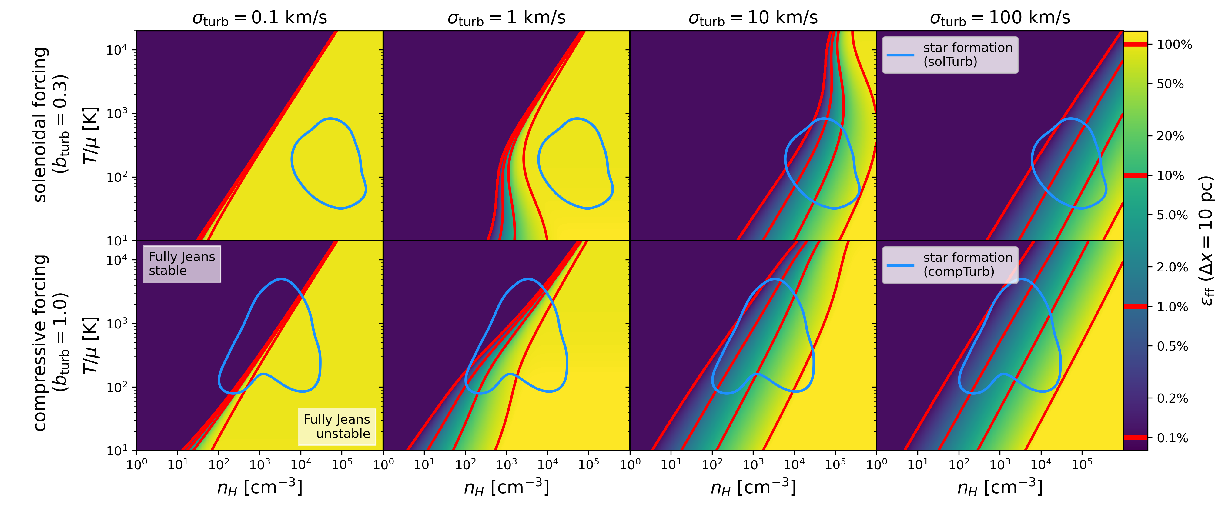
Figure 12: Local SFE as a function of temperature and Hydrogen number density in the MFF model (Eq. 22). Each column shows a different turbulent velocity dispersion. The top row is the solenoidal forcing limit ($b_{\rm turb}=0.3$) and the bottom row is the compressive forcing limit ($b_{\rm turb}=1.0$). The resolution scale is set to its minimum value $\Delta x=10~{}{\rm pc}$ in our simulations, and we emphasize that the local SFE is a resolution-dependent quantity by definition. Iso-efficiency contours are shown in red for $\epsilon_{\rm ff}\in\{0.1\%,1\%,10\%,100\%\}$. When $\epsilon_{\rm ff}\sim 0\%$, the gas is Jeans stable. When $\epsilon_{\rm ff}=100\%$, the gas is fully Jeans unstable. In each panel, we overplot a blue contour outlining the region of phase space containing 90% of star formation events weighted by stellar mass in solTurb (top row) and compTurb (bottom row). The contours are smoothed by a $\sigma=10~{}{\rm px}$ Gaussian filter for ease of viewing. In general, the local SFE decreases with increasing turbulent velocity dispersion for the same gas conditions, except for gas conditions which are marginally Jeans stable in the compressive forcing limit.

In real galaxies, the relationship between the forcing of small-scale turbulence and large-scale galactic dynamics is complex. varTurb provides a first insight into how this could play out. Solenoidal forcing modes in the turbulence may be driven by the differential rotation within a disc, suppressing star formation in discs. Meanwhile, compressive forcing modes may be driven by SN explosions, galaxy-galaxy mergers (Renaud et al., 2014), or accretion (Mandelker et al., 2024), enhancing star formation in those environments.

Due to self-regulation (Sec. 4.1), the decrease in local SFE due to the high turbulence of Cosmic Dawn only has a weak effect on the stellar mass which ultimately forms. For turbulent velocity dispersions even larger than the typical values $\sigma_{\rm turb}\sim 40~{}{\rm km/s}$ in our simulated galaxies, the local SFE may drop enough to take the galaxy out of the self-regulated regime. In this case, the integrated SFE would begin to decrease in proportion to the decrease in local SFE.

4.5 Other early feedback processes

Our early feedback model only includes thermal pressure from photoionized gas (Sec. 2.5). However, early feedback processes also include FUV radiation pressure, multiply-scattered IR radiation pressure, and stellar winds. All of these processes can be treated self-consistently by coupling the hydrodynamics to a radiative transport solver, for example using RAMSES-RT (Rosdahl et al., 2013). However, this extra physics comes at a computational cost. In this work, we prioritized modeling a large parameter space and understanding the physics in the simplified case of pure hydrodynamics.

Previous results from RAMSES-RT give clues about how our results might be affected by a more realistic early feedback model. Rosdahl et al. (2015) use RAMSES-RT to study the effect of radiative processes in a Milky-Way-like galaxy. They find that photoionization-heating is the dominant form of early feedback. In their simulations, photoionization feedback suppresses star formation by preventing the formation of star-forming clouds rather than by destroying them.

In principle, IR radiation pressure feedback should become more important in the high-density environments of Cosmic Dawn. IR photons can be absorbed and reemitted by dust multiple times when the IR optical depth is high. Even though typical UV dust opacities are $\sim 100$ times greater than IR dust opacities (Semenov et al., 2003), the multiply-scattered IR photons collectively exert more radiation pressure than the singly-scattered FUV photons.

Rosdahl et al. (2015) admit that they may underestimate the impact of IR radiation pressure feedback because the densest gas clouds are unresolved by their $\Delta x_{\rm min}=10~{}{\rm pc}$ resolution. However, Menon et al. (2022) suggest that the effect IR radiation pressure feedback is mitigated by the presence of turbulence, even at high surface densities. The authors explain that in an inhomogeneous medium, photons preferentially escape through low-density channels, increasing the escape fraction. This matter-radiation anti-correlation has been previously discussed in the context of massive star formation (Krumholz et al., 2009; Rosen et al., 2016) and lower densities regimes (Skinner & Ostriker, 2015; Tsang & Milosavljević, 2018).

Matter-radiation anti-correlation might be even more important in MDGs compared to Milky-Way-like galaxies. Our simulations indicate that MDGs host strong turbulence $\mathcal{M}_{\rm turb}\sim 30$. The turbulence is particularly strong in the dense regions which contribute most to the optical depth. Strong turbulence provides more low-density channels through which radiation can escape. In addition, radiation pressure feedback might self-regulate by driving a Rayleigh-Taylor instability which enhances turbulent motions further (Krumholz & Thompson, 2012). Another consideration at Cosmic Dawn is the low dust-to-gas ratio, which may reduce the effectiveness of radiation pressure feedback (Menon et al., 2024).

In Figure 13, we show how these effect conspire to reduce the IR optical depth in our simulations. In the left panel, we do not account for matter-radiation anti-correlation. In the other panels, we account for matter-radiation anti-correlation using an effective optical depth in the solenoidal and compressive forcing limits (Appendix G).

In this calculation, we determine the IR opacity using $\kappa_{\rm IR}=\tilde{\kappa}_{\rm IR}(Z/Z_{\odot})$, where $\tilde{\kappa}_{\rm IR}$ is the IR opacity at solar metallicity. We have assumed that the dust-to-gas ratio scales linearly with metallicity, which may overestimate the opacity at low metallicity (Feldmann, 2015; Choban et al., 2022). The opacity to IR photons at solar metallicity is roughly constant $\tilde{\kappa}_{\rm IR}\sim 5~{}{\rm g/cm^{2}}$ in the dust temperature range $100~{}{\rm K}\lesssim T_{\rm dust}\lesssim 1200~{}{\rm K}$, and takes on smaller values outside of that range (Semenov et al., 2003), so we adopt this constant value for the opacity and ignore the temperature dependence.

We find that the galaxy is only optically thick to IR photons when we do not account for matter-radiation anti-correlation. This suggests that the low metallicities and strong turbulence in MDGs can effectively suppress radiation pressure feedback from multiply-scattered IR photons.

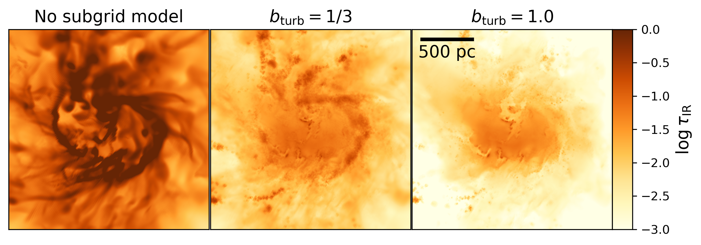
Figure 13: Logarithmic IR dust optical depth in a box of sidelength $2~{}{\rm kpc}$ around the most massive galaxy in the fiducial simulation, projected in the face-on direction. We compute the optical depth with no subgrid model (left panel), a solenoidal subgrid turbulence forcing model (middle panel), and compressive subgrid turbulence forcing model (right panel). In the latter two cases, the lower effective optical depth represents the matter-radiation anti-correlation i.e. radiation escapes preferentially through low density channels in the gas. The strong turbulence in MDGs makes the galaxy optically thin to IR photons when we account for matter-radiation anti-correlation.

Menon et al. (2023) find that although radiation pressure feedback cannot regulate star formation in clouds with surface densities $\Sigma_{\rm gas}\gtrsim 10^{3}~{}{\rm M_{\odot}/pc^{2}}$, the impulse of the FUV radiation force can launch outflows in clouds with surface densities $\Sigma_{\rm gas}\gtrsim 10^{5}~{}{\rm M_{\odot}/pc^{2}}$ which can be accelerated by IR radiation pressure. They propose that this mechanism can explain for the molecular outflows observed by Levy et al. (2021) in super-star clusters (SSCs) of NGC 253. It light of our previous arguments, it remains an open question whether this phenomenon could occur in MDGs.

Besides radiation pressure feedback, we also neglect the effect of stellar winds. Standard stellar mass-loss models, which likely overestimate the effect of stellar winds (Smith, 2014), predict that the momentum injected by stellar winds is at most comparable to that of radiation pressure from UV photons. Furthermore, line-driven winds from O-type stars are expected to weaken with decreasing metallicity. Based on these arguments, we do not think that stellar winds are a dominant feedback mechanism in MDGs, although this possibility should be investigated by future work.

4.6 Beyond the multi-freefall model

Our star formation recipe is based on the MFF model of Federrath & Klessen (2012). This model assumes that all of the gas in a gravitationally unstable gas cloud at the sonic scale forms stars. However, in reality the process of star formation is not 100% efficient even at the sonic scale. Previous observational (André et al., 2010) and theoretical (Matzner & McKee, 2000) work suggest that only $\epsilon_{\rm core}\sim 30-50\%$ of the gas in a collapsing prestellar core ends up in stars.

The MFF model can easily be modified by a prefactor $\epsilon_{\rm core}$ in Equation 22 which accounts for the efficiency of star formation at the sonic scale. Any value $\epsilon_{\rm core}<1$ would result in a lower local SFE $\epsilon_{\rm ff}$ for the same gas conditions. This is essentially the same effect as when we go from compressive to solenoidal turbulence forcing. solTurb indeed has a smaller local SFE than compTurb, but the integrated SFEs only differ by $\sim 5\%$ because our MDGs are in the self-regulated regime where their integrated SFEs are primarily determined by the strength of stellar feedback. Therefore, we expect that simulations with lower values of $\epsilon_{\rm core}$ will also have lower integrated SFEs, but only by a small factor.

The dependence of $\sigma_{s}$, the width of the subgrid density PDF, on the turbulent Mach number $\mathcal{M}_{\rm turb}$ (Eq. 12) comes from fitting a functional form to the small-scale turbulence simulations of Padoan & Nordlund (2011). Those simulations consider the steady state in a gas forced by the idealized Ornstein-Uhlenbeck process.

However, ISM turbulence is not a steady state and the forcing from the bulk velocity field and feedback processes is multi-scale and time-variable. Our turbulence forcing series are only a first pass at characterizing this uncertainty. In addition, the lognormal form of the subgrid density PDF is only an approximation (Federrath et al., 2010; Beattie et al., 2022). Deviations from a lognormal shape are more pronounced at high Mach numbers (Federrath & Klessen, 2012), such as those in MDGs. After a star-formation event, there may be a delay before the lognormal PDF can be reestablished by gravitational collapse which the model does not account for.

On top of these issues, the MFF model is fundamentally limited by its use of the density PDF alone to characterize the unresolved density field. The density PDF is a one-point statistical description that ignores spatial correlation. The same density PDF could be produced by numerous dense subsolar gas clumps or a single mass gas clump, which should physically correspond to different SFEs.

In a recent work, Hennebelle et al. (2024) develop a new star formation recipe they call the turbulent support (TS) model to address some of these shortcomings. The TS model substitutes the lognormal PDF in favor of the more complex Castaing-Hopkins PDF, which has been shown to produce better agreement in the high-Mach regime (Castaing, 1996; Hopkins, 2013).

Compared to the lognormal PDF, the Castaing-Hopkins PDF predicts lower amounts of gas at high densities, a consequence of small-scale turbulent pressure support. In addition, the TS model accounts for the spatial correlation of the unresolved density field, taking the power-law index of the mass function of self-gravitating clumps as a parameter. Finally, the TS model computes the freefall and PDF replenishment timescales and assumes star formation occurs on the minimum of the two.

Brucy et al. (2024) compare the predictions of the TS model to detailed turbulence simulations. Surprisingly, they find that the lognormal PDF reproduces the SFE in the high-Mach regime better than the Castaing-Hopkins PDF. It is unclear whether this discrepancy is physical or related to numerical dissipation in the turbulence simulations. For both PDFs, they find that the MFF tends to overpredict the SFE in the high-Mach regime (their Figure 14) in agreement with Hennebelle et al. (2024). In this regime, the turbulent Jeans length becomes larger than the turbulence injection scale. Because the turbulence injection scale is the maximum size at which turbulent structures can form, turbulence can no longer generate gravitationally unstable structures.

These arguments imply that that MFF may overestimate the SFR in MDGs. However, it’s worth noting that our simulations are at an intermediate resolution $\Delta x_{\rm min}\sim 10~{}{\rm pc}$ relative to the resolution of the detailed turbulence simulations of Brucy et al. (2024) at $\Delta x\sim 2~{}{\rm pc}$ and the size of the simulation domain $\Delta x\sim 1000~{}{\rm pc}$ on which they apply the TS model. It’s possible that although we use a more simple star formation recipe, we still capture some of the relevant behavior simply due to our high resolution. Future work should test the TS model at smaller scales to see whether it converges with the MFF model, and if so, at which scale.

Another aspect of star formation we have neglected is the equation of state (EOS), which we assume to be isothermal. Variations in the EOS can lead to changes in the density statistics (Passot & Vázquez-Semadeni, 1998; Li et al., 2003; Audit & Hennebelle, 2010). The simulations of Glover & Mac Low (2007a, b) indicate that the effective polytropic index may be sub-unity (soft EOS) in the density range $n_{\rm H}\sim 10-10^{4}~{}{\rm cm^{-3}}$ and super-unity (stiff EOS) at much higher densities $n_{\rm H}\gtrsim 10^{9}~{}{\rm cm^{-3}}$ where the gas starts to become optically thick (Masunaga & Inutsuka, 2000). In our simulations, the high-density tail of the subgrid density PDF enters this range (Fig. 17).

Federrath & Banerjee (2015) derive density variance vs. Mach number relations for multiple EOSs, analogous to Equation 12. At low Mach numbers, the density variance only depends weakly on the EOS. However, at high Mach numbers relevant to the conditions in MDGs, the density variance can increase significantly as the EOS becomes softer. Future detailed turbulence simulations should account for how the EOS changes at different density scales and produce a more accurate parameterization of the density distribution.

Our limited resolution requires that we represent stars as star cluster particles, where each particle represents a bound collection of individual stars. However, it is an open question what fraction of stars form in bound clusters. Observations of the local Universe suggest that the fraction is high, but perhaps not 100% (e.g. Lada & Lada, 2003; Porras et al., 2003; Bressert et al., 2010; Winston et al., 2020). Feedback from non-cluster stars might have an outsized impact on the ISM because such stars likely form in marginally star-forming conditions that are more diffuse.

When we form a star particle, the star particle inherits the velocity of the gas in its parent cell. However, the velocity of the star-forming cloud could deviate from this value on the scale of the turbulent velocity dispersion. Therefore, we might underestimate the diffusion of stars throughout the ISM and the fraction of SN explosions in non-star-forming environments.

4.7 Feedback modeling caveats

In dense regions when the SN cooling radius is unresolved, we model the SN explosion using momentum feedback. Without momentum feedback, the thermal energy injected by the SN would be unphysically radiated away before the snowplow phase of the SN blastwave.

However, by skipping the earlier phases of the SN explosion, we do not account for the effect of this heating on the star-forming cloud. This small-scale heating could allow SNe to more rapidly shut off star formation within a cloud. If we could resolve these scales, the SN delay time might become important to star formation as predicted in the FFB model (Dekel et al., 2023).

Our star formation recipe assumes that the density field has unresolved structure. Ideally, the same unresolved structure should be accounted for in our SN recipe. Specifically, the SN blastwave should sample the density PDF as it expands. Martizzi et al. (2015) simulate SN explosions in inhomogeneous media with a variety of turbulent Mach numbers. They find that as the Mach number increases, the SN explosion deposits its thermal energy and momentum at progressively larger radii (their Fig. 7). This effect increases the effectiveness of SN feedback. Future modeling should produce power law scalings similar to those in Martizzi et al. (2015) which incorporate the turbulent Mach number as a continuous parameter.

We determine the SN rate at each timestep assuming that SNe are uniformly distributed within the time interval between $\tau_{\rm start}$ and $\tau_{\rm end}$. This approach overestimates the SN rate at the beginning of the star cluster’s life, when the most massive and least abundant stars explode, and underestimates the SN rate at later times, when marginally massive and more abundant stars explode. In future work, we should adjust the SN rate over the course of the star cluster lifetime, following (Kimm et al., 2015).

In our model, SNe always occur at the location of the star cluster particle. However, the stellar population represented by a star cluster particle should have some spatial distribution. Weak two-body interactions can produce “walk-away” stars which slowly diffuse out of the cluster, or strong two-body interactions can produce “run-away” stars which are ejected out of the cluster at rapid velocities. Massive stars have short lifetimes, so walk-away massive stars may still go SN close to the cluster center, but run-away massive stars could go SN far from the cluster center. The fraction of massive stars ejected this way is enhanced relative to less massive stars because massive stars tend to concentrate at the centers of clusters where two-body encounters are more common (Oh & Kroupa, 2016).

If the gas density is more diffuse away from the cluster center, then the ejection of massive stars may decrease the mean gas density in which SNe occur, increasing the effectiveness of SN feedback. This effect was demonstrated in the radiation hydrodynamics simulations of Kimm & Cen (2014). However, the ejection of massive stars from the cluster might also decrease the timescale over which early feedback processes can suppress star formation. Detailed studies of the interaction between cluster dynamics and the ISM are needed to determine the ultimate effect on the SFE.

In the dense galactic environments of Cosmic Dawn, it may be possible for the dense shells of a SN blastwave to themselves be gravitationally unstable and trigger additional star formation. Using simple one-dimensional models, Nagakura et al. (2009) found that a triggered star formation can occur from a typical core-collapse SN in gas with density $n_{\rm H}\gtrsim 10^{3}~{}{\rm cm^{-3}}$. In our simulations, a significant fraction of SNe occur in this regime (Fig 8). Therefore, this effect may increase the SFR relative to what we predict. Secondary star formation might even be enhanced when accounting for small scale turbulence, because the conditions inside a SN blastwave are dominated by compressive forcing modes.

4.8 Miscellaneous considerations

Our simulations do not include a model for Pop III stars. At $z=9$, this is a good approximation, but our simulations begin at $z\sim 100$ and therefore they include the time period where Pop III stars dominate the cosmic star formation history $z\sim 15-20$ (see Klessen & Glover, 2023, for a review). Pop III stars with masses $140~{}M_{\odot}\lesssim m_{*}\lesssim 260~{}M_{\odot}$ are expected to undergo pair-instability SNe, which have energies $100\times$ that of more standard core-collapse SN, leading to more effective SN feedback.

Even after Pop III star formation ceases, stars forming in low metallicity $Z\lesssim 3\%~{}Z_{\odot}$ environments could form directly from atomic gas due to the discrepancy between the thermal and chemical equilibrium timescales (Glover & Clark, 2012; Krumholz, 2012). The formation timescale for ${\rm H}_{2}$ is slow at low metallicities due to the lack of dust grain surfaces the catalyze the reaction, so the molecular fraction remains small until the density rises high enough to form $H_{2}$ via 3-body reactions. If the gas surrounding a young massive star is primarily atomic Hydrogen, the effect of photoionization feedback may be enhanced due to the lower ionization energy relative to molecular Hydrogen. More detailed studies are needed to explore these effects, especially in less massive haloes at Cosmic Dawn, which may be less rapidly enriched by metals.

As discussed in Section 1, some MDGs show evidence of AGN activity. AGN might provide an additional source of feedback which we do not consider. From a theoretical perspective, the formation mechanisms of supermassive BHs (SMBHs) is an open question. It is typically assumed that SMBHs form from massive BH seeds, which grow by accretion and mergers. As pointed out by Dekel et al. (2023), the enhanced SFE in massive $z\sim 10$ galaxies might suppress accretion onto the BH by consuming most of the gas in star formation. On the other hand, the inefficiency of feedback may enhance accretion of the residual gas. Future simulations could address the question of BH growth and AGN feedback by using the sink particle functionality already available in RAMSES.

The multiple non-linear coupled PDEs in our galaxy simulations form a chaotic system, and therefore our results are subject to chaotic variance, seeded by truncation errors and random algorithmic elements. Genel et al. (2019) found that global properties of a single galaxy can vary on a level of $\sim 2-25\%$ due to chaotic variance, depending on the property in question. In a similar analysis, Keller et al. (2019) concluded that differences $\lesssim 20\%$ in time-average SFRs between different galaxy simulations require statistical evidence to show that it is not due to stochasticity, with mergers being a particularly large source of chaos. Ideally, we could run multiple copies of each simulation to quantify the range of chaotic variance, but this was impossible due to computational cost. Most of our conclusions are based on integrated quantities or statistical analyses, so we believe that our results are robust to chaotic variance, but we do not have data to confirm this.

4.9 Observational implications

4.9.1 SFR indicators

Caplar & Tacchella (2019) point out that when the SFR is determined from observations, one must rely on tracers such as IR, UV, and emission lines. These tracers do not reflect the instantaneous SFR because they have different contributions from stars of different ages. To predict what the star formation history looks like as seen by a given indicator, we convolve the intrinsic SFR with the response function of that indicator.

Using the Flexible Stellar Population Synthesis (FSPS) code (FSPS, Conroy et al., 2009), we estimate the response function for two star formation indicators: the H$\alpha$ emission line and the JWST f200w filter. At $z=9$, the H$\alpha$ line is redshifted to $\lambda=5.9~{}{\rm\mu m}$, which is outside the spectral range of JWST’s NIRSpec instrument. However, we found that viable emission line indicators such as H$\beta$ and the OIII lines produce similar response functions to H$\alpha$. At $z=9$, JWST’s f200w and f277w filters probes mid-UV and near-UV frequencies respectively. We find that the f277w filter produces a similar response function to the f200w filter.

We assume a redshift $z=9$, a Chabrier IMF (Chabrier, 2003), and a metallicity $Z=0.331~{}Z_{\odot}$, equal to the median metallicity of stars in our fiducial simulation. FSPS also includes dust and nebular emission models. FSPS has been extensively calibrated against observations in the low redshift Universe (Conroy & Gunn, 2010). There may be large systematic errors at $z\sim 10$, which we ignore for the sake of qualitative argument.

We plot the response functions in the right panel of Figure 14. H$\alpha$ responds rapidly on a timescale of $\sim 3~{}{\rm Myr}$, while the JWST f200w filter responds on longer timescales of $\sim 10~{}{\rm Myr}$, but with small contributions on timescales as long as $\sim 100~{}{\rm Myr}$. Note that our response function for the JWST f200w filter is only valid at $z=9$. At higher redshifts, the JWST f200w filter responds slightly faster e.g. on timescales $\sim 5~{}{\rm Myr}$ for $z=19$. The OIII$\lambda$4960 line, another plausible emission line indicator, has a similar response function to H$\alpha$. Likewise, the JWST f277w filter, another plausible photometric indicator, has a similar response function to the JWST f200w filter.

In the left panel of Figure 14, we show the SFR as a function of time for the fiducial simulation, including both the intrinsic SFR and the SFR inferred by H$\alpha$ and JWST f200w star formation indicators. The H$\alpha$ SFR is similar in magnitude to the intrinsic SFR, but the JWST f200w SFR is systematically smaller, resulting from the long-timescale contributions which sample earlier times when the SFR was lower. This effect is a consequence of the rapid increase in the mean SFR as a function as time in this epoch. Both SFR indicators hide the intrinsic variability in the SFR on short timescales $\lesssim 1~{}{\rm Myr}$, suggesting that such variability may be difficult to observe in practice.

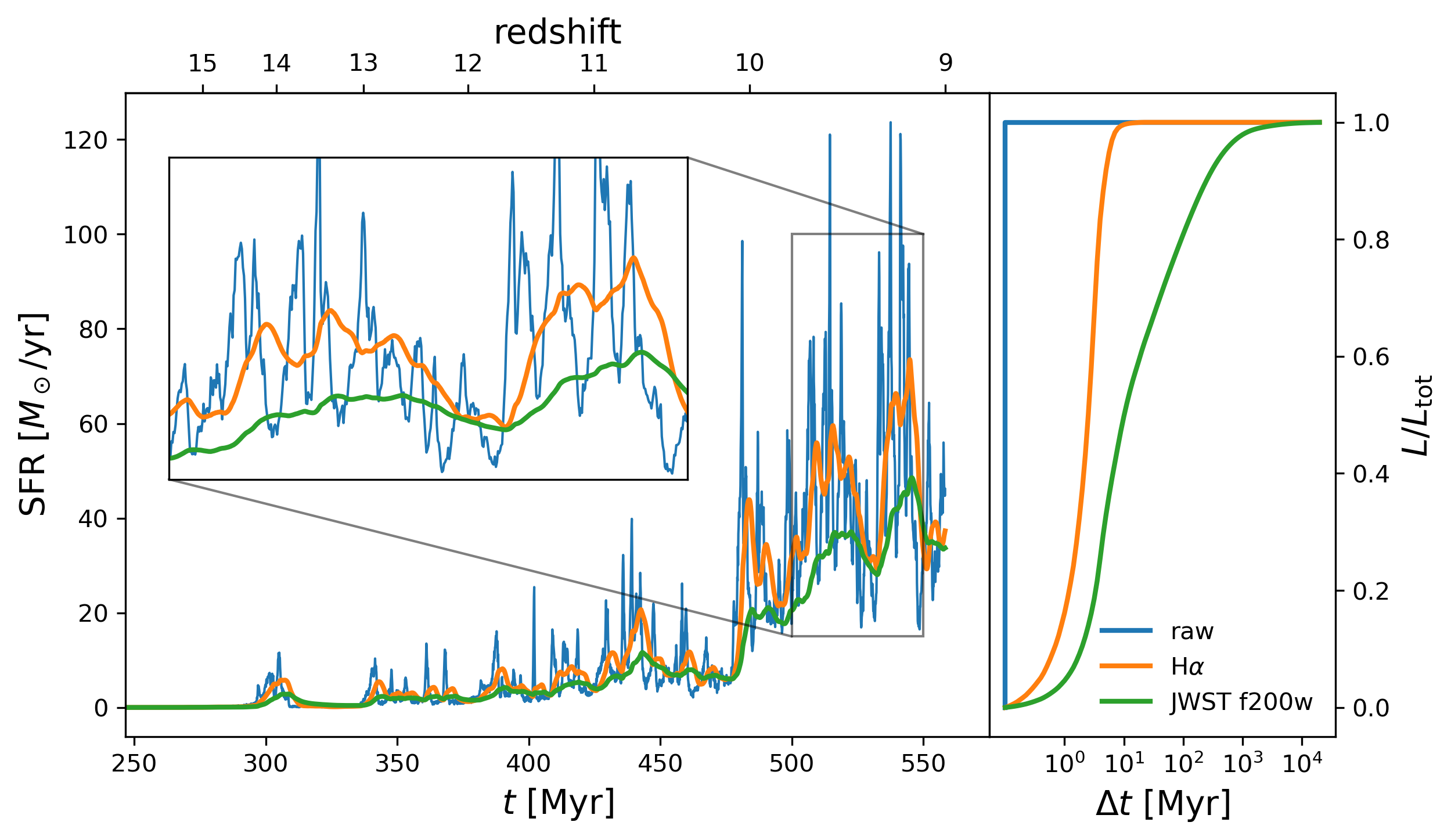
Figure 14: SFR as a function of time (left panel) for the fiducial simulation, including both the intrinsic SFR (blue) and the SFR inferred by H$\alpha$ (orange) and the JWST f200W filter (green). An inset plot shows a zoom to highlight how the indicators respond to short-timescale variability. In the right panel, we show the cumulative luminosity for a given indicator as a function of time. The H$\alpha$ SFR is similar in magnitude to the intrinsic SFR, but the JWST f200w SFR is systematically smaller, resulting from the long-timescale contributions which sample earlier times when the SFR was lower.

4.9.2 Turbulence on observations

The strong turbulence in MDGs may influence our interpretation of observations. In Appendix G, we show that matter-radiation anti-correlation decreases the photon mean free path by a factor proportional to $\mathcal{M}_{\rm turb}^{-2}$. This makes the galaxy less opaque to all photons, not just the IR photons discussed in Section 4.5. We refer to this effect as turbulent deattenuation.

If turbulent deattenuation affects all wavelengths equally, than it would be degenerate with the normalization of the galaxy spectrum and may cause spectral energy distribution (SED) fitting codes to overestimate the stellar mass and SFR. However, the degeneracy could be broken if the turbulent Mach number can be measured from observations.

In the local Universe, this can be done with spatially resolved measurements of the velocity dispersion and temperature. For example, Schneider et al. (2013) used the Herschel Space Observatory’s (Pilbratt et al., 2010) high angular resolution measurements of ${}^{12}{\rm CO}~{}1\to 0$ line widths and dust temperatures to estimate the turbulent Mach number in local molecular clouds. The turbulent Mach number can also be measured using spatially resolved column density maps to estimate the fractal dimension of the density field (Beattie et al., 2019).

The measurement becomes more difficult at Cosmic Dawn, where spatially resolved measurements are not possible, even with high angular resolution, unless the galaxy is strongly lensed. In measurements of the velocity dispersion which are not spatially resolved, contributions from turbulence and from the bulk motion of the gas must be separated, which may not always be possible.

4.9.3 Stellar masses and SFRs

In Figure 15, we plot the stellar mass and SFR in our fiducial simulation as a function of redshift in red. We also plot our epistemic uncertainty, the range of stellar masses and SFRs across simulations in the early feedback and turbulence forcing series. The stellar mass and SFR data for each simulation are available on the Princeton Research Data Service (Andalman & Teyssier, 2024).

In blue, green, and orange, we show estimates of stellar mass and SFR from JWST NIRSpec spectropscopy and NIRCam photometry for a selection of luminous galaxies from the JWST Advanced Deep Extragalactic Survey (JADES Eisenstein et al., 2023), Cosmic Evolution Early Release Science (CEERS Finkelstein et al., 2023a, ERS-1345), and (COSMOS-Web Casey et al., 2023, GO#1727). We source our data for each survey from Harikane et al. (2024), Carniani et al. (2024), and Casey et al. (2024) respectively. This selection includes the most luminous and high redshift galaxies spectroscopically confirmed at the time of writing, such as GS-z11-0, GS-z14-0, and GS-z14-1.

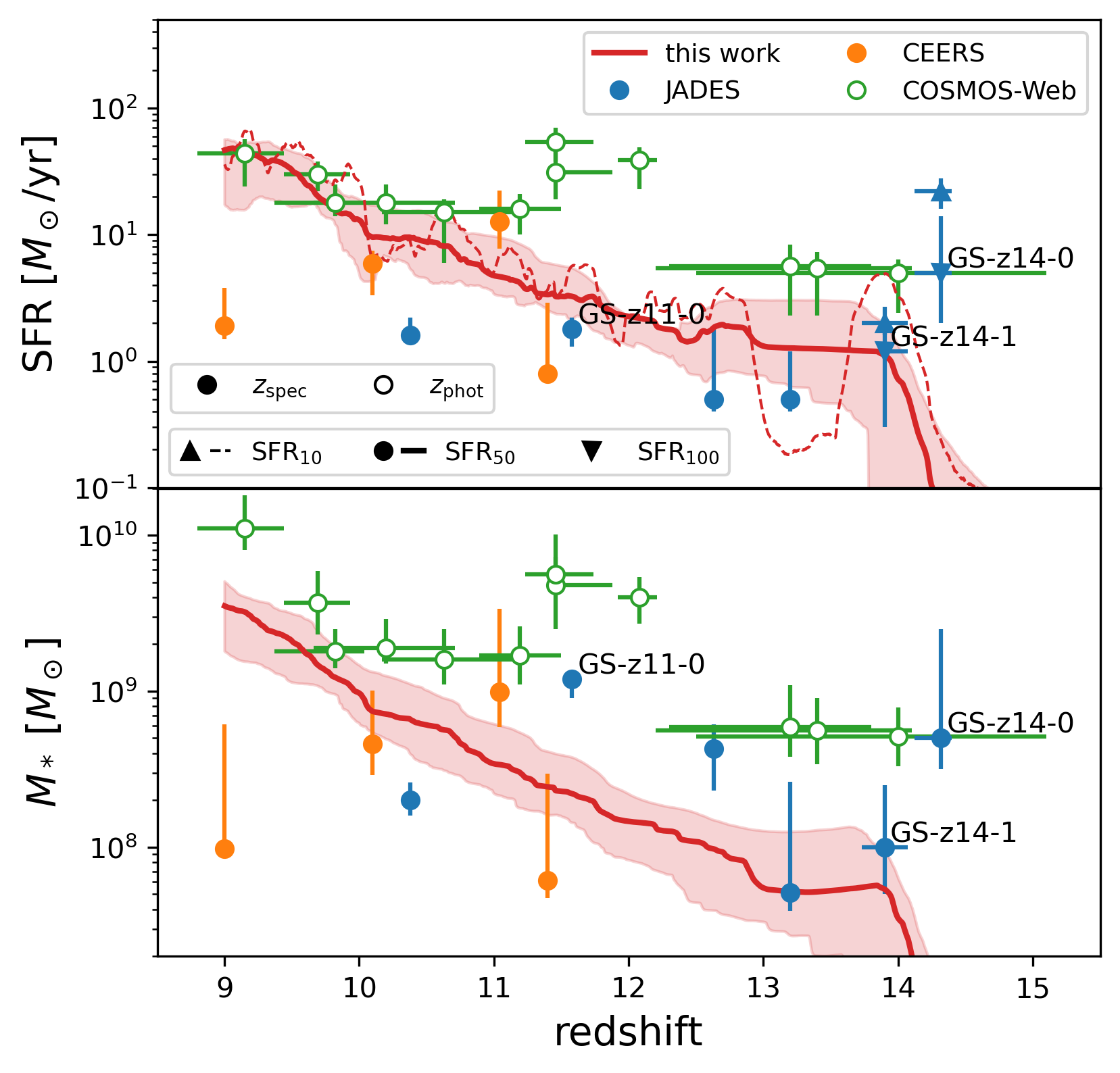
Figure 15: SFR (top panel) and stellar mass (bottom panel) as a function of time in our simulations (red) and a selection of the most luminous galaxy candidates at Cosmic Dawn in various surveys, including JADES (blue), CEERS (orange), and COSMOS-Web (green). The solid red line shows data from our fiducial simulation and the shaded area includes the range of values from lowPhot, highPhot, solTurb, and varTurb. Galaxy candidates which are not spectroscopically confirmed are marked with an open circle. SFR is averaged over $10~{}{\rm Myr}$ (up triangle, solid line), $50~{}{\rm Myr}$ (circle), and $100~{}{\rm Myr}$ (down triangle, dashed line). The stellar mass and SFR data for each simulation are available on the Princeton Research Data Service (Andalman & Teyssier, 2024).

Ideally, we should only compare our simulated galaxy to observed galaxies whose halo mass matches that of our simulated galaxy at the appropriate redshift. However, the star-to-halo mass ratio at Cosmic Dawn is not well-constrained, since it depends on the integrated SFE. As argued in Section 1, the most extreme objects discovered at Cosmic Dawn in current surveys should have halo masses in around the value $M_{\rm halo}\sim 10^{11}~{}M_{\odot}$ for our simulated galaxy. However, surveys which sample a larger volume, like COSMOS-Webb, probably include more massive haloes $M_{\rm halo}\geq 10^{11}~{}M_{\odot}$ which naturally have larger stellar masses and SFRs.

The COSMOS-Webb candidates are not spectroscopically confirmed, indicated by open circles in the plot, so their redshifts should be taken with caution. Previous work suggests that photometric estimates of redshift systematically overestimate redshift for galaxies at Cosmic Dawn (e.g. Fujimoto et al., 2023, Fig. 4). Even when spectra are available, stellar masses and SFRs are typically estimated using spectral fitting codes like Bagpipes (Carnall et al., 2018) and Prospector-$\alpha$ (Leja et al., 2019). However, at Cosmic Dawn, NIRSpec data provides very little constraints on dust-obscured star formation or the presence of an AGN, which would artificially decrease and increase stellar population estimates respectively.

The crude comparison in Figure 15 is reasonable because the stellar masses and SFRs inferred from observations are already highly model-dependent. We are only suggesting that our simulated galaxies are in the ballpark of stellar masses and SFRs of the MDGs seen by JWST. Future work could make this comparison more quantitative using abundance matching and accounting for the effects of cosmic variance (Kragh Jespersen et al., 2024), but a more detailed approach may not be justified until the observational data are better understood.

More observational evidence for MDGs are found at Cosmic Noon ($z\sim 3$), near the peak of the cosmic SFR density, where a population of massive quiescent galaxies (MQGs) have emerged (Glazebrook et al., 2017; Valentino et al., 2020; Antwi-Danso et al., 2023; Carnall et al., 2023, 2024; de Graaff et al., 2024a; Glazebrook et al., 2024). These galaxies typically have large stellar masses $M_{*}\gtrsim 10^{10}~{}M_{\odot}$ and low specific SFRs $\lesssim 0.2$. Recently, Weibel et al. (2024) reported the discovery of a MQG at $z=7.3$ confirmed spectroscopically with JWST NIRSpec as part of the Cycle 2 program of RUBIES (GO#4233) with a stellar mass $M_{*}\sim 10^{10}~{}M_{\odot}$.

Detailed modeling of MQG spectra suggests that MQGs must have formed the bulk of their stellar populations within the first billion years of cosmic history in short, extreme starbursts lasting hundreds of ${\rm Myr}$ at most Weibel et al. (e.g. 2024). This is qualitatively consistent with our simulated MDGs, hinting that MDGs could be the progenitors of MQGs. Future work should extend run simulations out to lower redshift to investigate this possibility. Cosmological simulations tend to underproduce MQGs at high redshift (Alcalde Pampliega et al., 2019; Merlin et al., 2019), so they have been understudied in the theoretical galaxy formation community.

5 Conclusions and Future Work

In this work, we run zoom-in simulations of a MDG ($M_{\rm halo}=10^{11}~{}M_{\odot}$, $z=9$) using the cosmological hydrodynamics code RAMSES at an effective resolution $\simeq 10~{}{\rm pc}$. Our simulations capture the unique regime of high densities $\Sigma_{\rm gas}\sim 10^{4}~{}{\rm M_{\odot}/pc^{2}}$, $n_{\rm H}\sim 3\times 10^{3}~{}{\rm cm^{-3}}$ where star formation is expected to be enhanced. Our suite of simulations vary in the details of their star formation and feedback recipes, allowing us to investigate the connection between global SFE and local gas conditions. Our fiducial simulation uses a physically-motivated, turbulence-based, multi-freefall model of star formation, avoiding ad hoc extrapolation from lower redshifts.

We summarize our main findings in bullet points:

• Star formation efficiencies: The high densities $\Sigma_{\rm gas}\sim 10^{4}~{}{\rm M_{\odot}/pc^{2}}$, $n_{\rm H}\sim 3\times 10^{3}~{}{\rm cm^{-3}}$ in star-forming regions of MDGs naturally result in efficient star formation, with a local SFE $\epsilon_{\rm ff}\sim 10-20\%$ and an integrated SFE $\epsilon_{\rm int}\sim 10-30\%$.

• Galaxy structure: Our simulated galaxies form a thick, rotationally-supported disc. For cold gas, the disc radius is $R_{\rm gas}\sim 700~{}{\rm pc}$ and the scale height is $H/R\sim 0.5$. For stars the disc radius is $R_{\rm gas}\sim 400~{}{\rm pc}$ and scale height is $H/R\sim 0.25$. The gas scale height calculation for the disc may be artificially inflated by accretion of cold gas. The baryonic mass is organized into dense, cold, and turbulent clumps of diameter $\sim 100~{}{\rm pc}$ where most of the star formation occurs, although the size of these clumps may be an artifact of our $\sim 10~{}{\rm pc}$ resolution. These discs may have analogues in the discs of star-forming galaxies at cosmic noon, which are better studied in theory and observation.

• Star formation history and variability The stellar mass in the MDG increases in proportion to the accretion rate onto the halo i.e. nearly exponential growth for $z\geq 9$. The SFR fluctuates on various timescales. The Fourier transform of the SFR may encode information about the typical density of star formation $n_{\rm H}\sim 3\times 10^{3}~{}{\rm cm^{-3}}$ and the typical lifetime of star-forming clouds $\tau_{\rm cl}\sim 10~{}{\rm Myr}$.

• Stellar feedback: Our implementation of stellar feedback is crude, but our preliminary results suggest that stellar feedback in MDGs is weak due to the high density conditions. This is consistent with the general prediction of the FFB scenario, despite the fact that our current simulations don’t yet resolve the SN cooling radius and the star-forming clusters where FFB is expected to occur. Weak feedback can be partially mitigated by photoionization from massive stars, which decrease the density around SN explosions. However, even in our strongest photoionization feedback model the integrated SFE is still high $\geq 10\%$.

• Self-regulation: One might think that the weak feedback in MDGs cannot regulate star formation. However, we show that star formation is still regulated by feedback due to the high local SFE. As a result, the global SFE is nearly independent of the local SFE and depends inversely on the strength of ejective feedback.

• Metal enrichment: Similar to the global SFE, gas metallicity depends inversely on the strength of ejective feedback. By $z=9$, SN feedback enriches our simulated galaxies to a significant fraction of solar metallicity.

• Turbulence: Turbulence generally decreases the local SFE for the same gas conditions due to turbulent pressure support. The strong turbulence $\mathcal{M}_{\rm turb}\sim 30$ in MDGs prevents star-forming clouds from catastrophically collapsing. However, turbulence is not strong enough to take MDGs out of the self-regulated regime, so it has only a weak effect on global and integrated SFEs.

• Matter-radiation anti-correlation Radiation tends to move through low-density channels in the density field, so strong turbulence decreases the effective optical depth by a factor proportional to $\mathcal{M}_{\rm turb}^{-2}$. This effect may reduce the ability for radiation pressure feedback to suppress star formation and cause SED fitting codes to overestimate stellar masses and SFRs.

• Comparison to observations: Our simulated galaxies are in the ballpark of the estimated stellar masses and SFRs of the MDGs observed by JWST.

Our study is the first step towards understanding efficient star formation in MDGs. Our treatment of stellar feedback is crude due to the limitations of our effective resolution $\sim 10~{}{\rm pc}$ in a pure hydrodynamics simulation (i.e. no radiation). Although these factors affect the accuracy of our results, they also make the simulations easier to interpret by simplifying the physics. We will use the insights from this work to make informed choices about more computationally expensive future simulations which capture more of the physics.

The interplay between photoionization and SN feedback in our simulations suggests that early feedback is important in MDGs, even when it cannot suppress star formation directly. In future simulations, we will model early feedback in more detail using RAMSES-RT, including explicit models for photoionization, radiation pressure, and stellar winds. These models should account for the effect of strong turbulence, which can decrease the effective opacity (Sec. 4.9.2). Using RAMSES-RT will also enable a more self-consistent treatment of the extragalactic radiation field.

The high densities in our simulations mean that we do not resolve the scale of star-forming clouds, which can be roughly approximated by the Jeans radius $R_{\rm J}=c_{\rm s}/\sqrt{G\rho}$. For a cloud at the Hydrogen ionization temperature $T\sim 10^{4}~{}{\rm K}$ and a density given by the median star-forming density of our fiducial simulation $n_{\rm H}\sim 3\times 10^{3}~{}{\rm cm^{-3}}$, the Jeans radius is $R_{\rm J}\sim 20~{}{\rm pc}$, and the cloud will only be resolved by eight cells $\Delta x_{\rm min}\sim 10~{}{\rm pc}$. For a lower temperature given by the median star-forming temperature of our fiducial simulation $T\sim 300~{}{\rm K}$, the Jeans radius is $R_{\rm J}\sim 3~{}{\rm pc}$, and the cloud will not be resolved at all. The addition of 3 AMR levels would give $\Delta x_{\rm min}\sim 1~{}{\rm pc}$, resulting in fully resolved star-forming clouds. A high resolution would also solve the problem of unresolved HII regions, revealing the multi-phase structure of the ISM.

There are many other avenues for future work, including (i) exploring the growth of black holes and impact of AGN on star formation in MDGs and (ii) running simulations beyond Cosmic Dawn to investigate whether our MDGs could be the progenitors of massive quiescent galaxies at lower redshifts.

Data Availability

The simulations in this work were run on Stellar cluster at Princeton University. Each simulation contains approximately $1.3~{}{\rm Tb}$ of data. Access to this data can be provided upon request to the corresponding author.

A dataset containing the stellar mass and SFR as a function of proper time and redshift for the fiducial model and models lowPhot, highPhot, solTurb, and varTurb are provided on the Princeton Research Data Service (Andalman & Teyssier, 2024) under the Creative Commons Attribution 4.0 International (CC-BY-4.0) license. This dataset may be useful for comparing our simulated MDGs results to other simulated or observed MDGs.

Movies of the simulations are publicly available on YouTube (https://tinyurl.com/53xxm3r2).

Appendix A Simple estimate for baryon surface density

We define a dark matter halo as a sphere about a density peak with mean overdensity $\Delta\simeq 200$ above the cosmological background $\rho_{\rm crit}$, following the standard definition from the spherical-collapse model (Gunn & Gott, 1972). This implies a matter density inside the halo of

$$\rho_{\rm halo}=\Delta\rho_{\rm crit,0}\Omega_{\rm m,0}(1+z)^{3}$$ (51)

and a halo radius

$$R_{\rm halo}=\left(\frac{M_{\rm halo}}{(4\pi/3)\rho_{\rm halo}}\right)^{1/3}=\left(\frac{M_{\rm halo}}{(4\pi/3)\Delta\rho_{\rm crit,0}\Omega_{\rm m,0}}\right)^{1/3}(1+z)^{-1}$$ (52)

where $\rho_{\rm crit,0}=3H_{0}^{2}/(8\pi G)$ is the critical density of the Universe at redshift $z=0$.

Following Dekel et al. (2013), we assume that the radius of the galactic disc scales with the halo radius via a contraction factor $\lambda$

$$R_{\rm gal}=\lambda R_{\rm halo}$$ (53)

Based on tidal-torque theory, Dekel et al. (2013) argue that the average $\lambda$ is similar to the halo spin parameter, with typical value $\lambda\simeq 0.05$ (e.g. Bullock et al., 2001).

We further assume that the baryon mass in the galactic disc approximately equal to the total accreted baryon mass,

$$M_{\rm gas}=f_{\rm b}M_{\rm halo}$$ (54)

Under these assumptions, the baryon surface density $\Sigma_{\rm gas}$ in a galaxy is given by

$$\Sigma_{\rm gas}=\frac{M_{\rm gas}}{\pi R_{\rm gal}^{2}}=\frac{f_{\rm b}M_{\rm halo}^{1/3}}{\pi\lambda^{2}}\left(\frac{4\pi}{3}\Delta\rho_{\rm crit,0}\Omega_{\rm m,0}\right)^{2/3}(1+z)^{2}$$ (55)

We use Equation 55 to estimate the baryon surface density in a galaxy as a function of redshift and the mass of its host halo in Figure 1.

Appendix B Contribution of massive stars to photoionization

The average rate of Hydrogen-ionizing photons emitted per stellar mass depends on both the IMF $\xi(m)$ and the rate of ionizing photon emission as a function of stellar mass $Q(m)$. The latter has empirical constraints from the local Universe.

In Fig. 16, we plot data from Table 15.1 of Draine (2011) and fits to the functional form $Q(m)\sim am^{b}+c$ using the least-squares method. Across luminosity classes, only stars with masses $m\gtrsim 20~{}M_{\odot}$ make significant contributions to the ionizing photon production, making photoionization feedback sensitive to the high-mass end of the IMF.

This uncertainty motivates the large range of values for $M_{\rm cl}$ in our early feedback series. The crudeness of our early feedback recipe is a reflection of the limitations of a pure hydrodynamics simulation and large uncertainties at Cosmic Dawn.

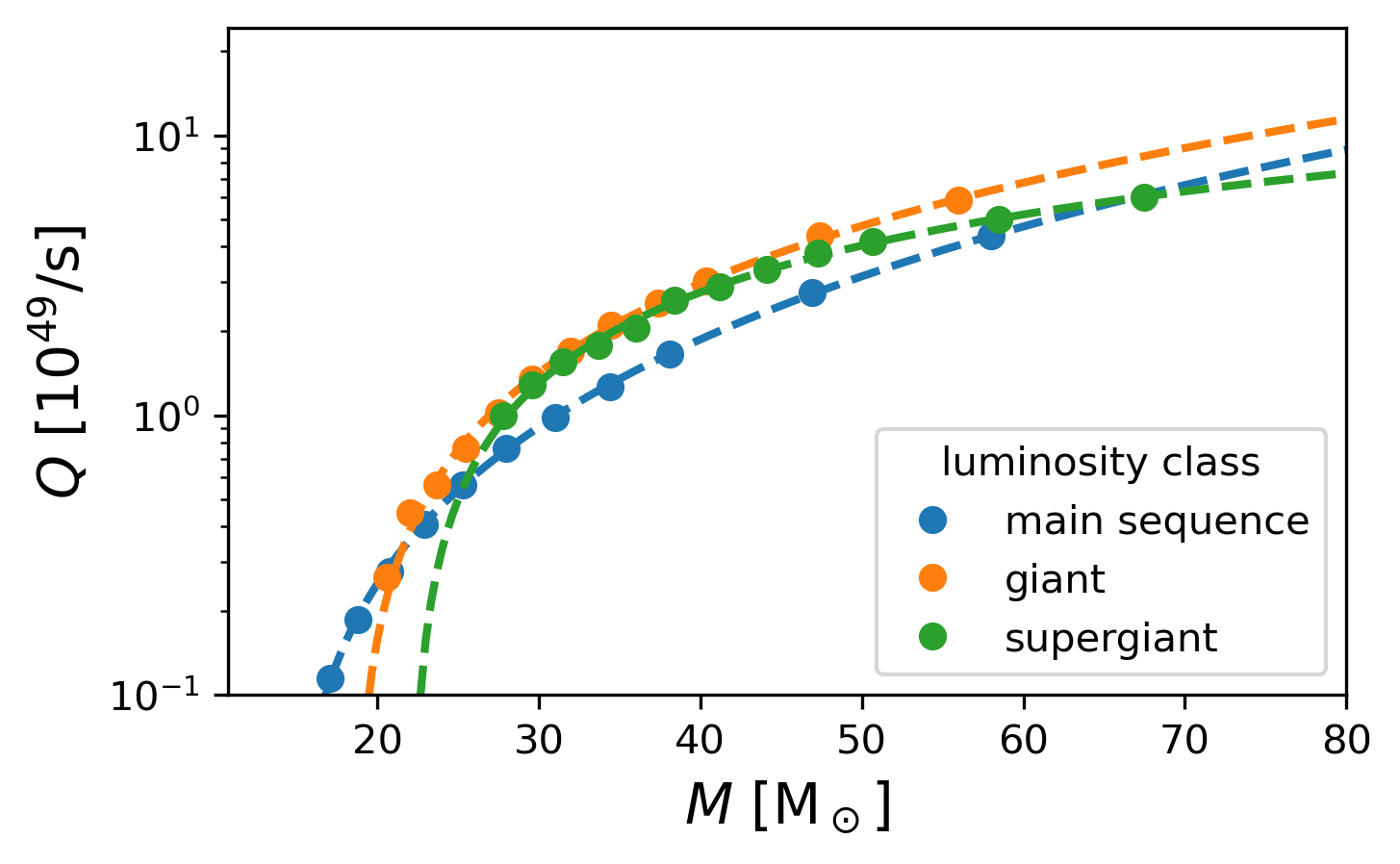
Figure 16: The rate of ionizing photon emission as a function stellar mass for massive stars on the main sequence (blue), the giant branch (orange), and the supergiant branch (green). The dots are data from Draine (2011), Table 15.1 and the dashed lines are fits to the functional $Q(M)\sim aM^{b}+c$.

Appendix C Calculation of net angular momentum

In Figure 3, we show face-on and edge-on projections of the galaxy. In this section, we describe the procedure for computing the direction of net angular momentum required to generate these projections.

First, we estimate the bulk velocity $\mathbf{v}_{\rm bulk}$ of the galaxy as the mass-weighted average velocity in a $3~{}{\rm kpc}$ sphere with center $\mathbf{r}_{\rm c}$, the center of the galaxy. Contributions from stars and gas are included in the mass weight. The typical bulk velocity of the galaxy relative to our grid is on the order of hundreds of ${\rm km/s}$.

Next, we compute the direction of the net angular momentum of the galaxy $\hat{\mathbf{\boldsymbol{\Omega}}}$, which is in general not aligned with the Cartesian simulation grid. We estimate the direction of the net angular momentum as the mass-weighted sum of the specific angular momentum in a $3~{}{\rm kpc}$ sphere with center $\mathbf{r}_{\rm c}$, where the specific angular momentum is given by $\mathbf{l}=(\mathbf{r}-\mathbf{r}_{\rm c})\times(\mathbf{v}-\mathbf{v}_{\rm bulk})$. Contributions from stars and gas are included in the mass weight.

We define a primed coordinate system $\mathbf{r}^{\prime}$ with origin $\mathbf{r}_{\rm c}$ and $z$-axis parallel to $\hat{\mathbf{\boldsymbol{\Omega}}}$. By projecting parallel to $\hat{\mathbf{z}}^{\prime}$, we can view the galaxy face-on. Likewise, by projecting parallel to $\hat{\mathbf{x}}^{\prime}$ or $\hat{\mathbf{y}}^{\prime}$, we can view the galaxy edge-on.

In Section 3.2, we used the scale height to quantify the disciness of the galaxy. We compute the scale height using an iterative method based on Appendix B of Mandelker et al. (2014).

Let $M_{\rm cyl}(H,R)$ denote the mass contained inside a cylinder of height $H$ and radius $R$ with axis along $\hat{\mathbf{z}}^{\prime}$ and center $\mathbf{r}_{\rm c}$. We start with an initial guess for the disc height $H$ and an upper bound on the disc radius $R_{\rm max}$. Then, we iterate the following steps until convergence to a less than 1% change between iterations in $H$ and $R$:

1. Determine the radius $R$ such that $M_{\rm cyl}(H,R)=fM_{\rm cyl}(H,R_{\rm max})$.

2. Determine the height $H$ such that $M_{\rm cyl}(H,R)=fM_{\rm cyl}(R,R)$.

We set the initial disc height $H=500~{}{\rm pc}$ and the upper bound on the disc radius $R_{\rm max}=1~{}{\rm kpc}$. However, our results are not sensitive to changes in these parameters by factors of a few. We chose a mass fraction $f=85\%$ consistent with Mandelker et al. (2014). The calculation can be repeated separately for cold gas and stars. We only include gas with temperatures $T/\mu\leq 10^{4}~{}{\rm K}$ to exclude outflows and accreting gas.

To compute the ratio of the rotation velocity to the radial velocity dispersion, we first compute the relative velocity components in the primed coordinate system

$$\Delta v_{x^{\prime}}=\ (\mathbf{v}-\mathbf{v}_{\rm bulk})\dotproduct\hat{\mathbf{x}}^{\prime},\quad\Delta v_{y^{\prime}}=(\mathbf{v}-\mathbf{v}_{\rm bulk})\dotproduct\hat{\mathbf{y}}^{\prime}$$ (56)

In cylindrical polar coordinates $(s,\varphi,z)$, this becomes

$$\Delta v_{s^{\prime}}=s^{-1}(x^{\prime}\Delta v_{y^{\prime}}-y^{\prime}\Delta v_{x^{\prime}}),\quad\Delta v_{\varphi^{\prime}}=s^{-1}(x^{\prime}\Delta v_{x^{\prime}}+y^{\prime}\Delta v_{y^{\prime}})$$ (57)

The ratio of the rotation velocity to the radial velocity dispersion at cylindrical radius $s^{\prime}$ is

$$\frac{v_{\rm rot}}{\sigma_{r}}(s^{\prime})=\expectationvalue{\Delta v_{\varphi^{\prime}}}_{\rho}(s^{\prime})\left(\expectationvalue{(\Delta v_{s^{\prime}})^{2}}_{\rho}(s^{\prime})-\expectationvalue{\Delta v_{s^{\prime}}}_{\rho}^{2}(s^{\prime})\right)^{-1/2}$$ (58)

where $\expectationvalue{\cdot}_{\rho}(s^{\prime})$ denotes a density-weighted average over a cylindrical shell at cylindrical radius $s^{\prime}$.

We use cylindrical shells of width $\Delta s^{\prime}=25~{}{\rm pc}$ for $s\leq R$ and height $H$. The overall ratio of the rotation velocity to the radial velocity dispersion is the average over cylindrical shells, weighted by the mass of each shell. The ratio can be computed separately for gas and stars using the corresponding disc dimensions.

We adopt the notation $v_{\rm rot}/\sigma_{r}$ to be consistent with previous literature in the main body of the paper. However, we emphasize that the radial velocity dispersion is computed in cylindrical polar coordinates, not spherical polar coordinates.

Appendix D Calculation of summary statistics

In Section 3.5, we used various summary statistics to compare our simulations, including the total stellar mass $M_{*}$ in the galaxy at $z=9$, the average SFR over the last $50~{}{\rm Myr}$ at $z=9$ ${\rm SFR}_{50}$, the integrated SFE $\epsilon_{\rm int}$, the median local SFE ${\rm med}(\epsilon_{\rm ff})$, and the outflow efficiency $\eta$. We compute each statistic using a box $\mathcal{B}$ of side length $5~{}{\rm kpc}$ centered on the galaxy. In our simulations, this box contains $\sim 1/3$ of the total stellar mass in the entire volume.

We compute the stellar mass by summing the star particle mass within the box at $z=9$:

$$M_{*}=\sum_{\mathbf{r}_{k}\in\mathcal{B}}m_{k}$$ (59)

where $\mathbf{r}_{k}$ and $m_{k}$ are the position and mass respectively of star particle $k$.

The average SFR over the last $50~{}{\rm Myr}$ at $z=9$ (denoted here as ${\rm SFR}_{50}$) is given by

$${\rm SFR}_{50}=\frac{1}{50{\rm Myr}}\int_{50{\rm Myr}}^{0}\dot{M}_{*}(t_{9}-t)\differential t$$ (60)

where $t_{9}$ is the proper time at $z=9$.

We compute the SFR as a function of time by binning the star particle mass within the box by time of birth:

$$\widetilde{\dot{M}}_{*}(t)=\frac{1}{\Delta t}\sum_{\begin{subarray}{c}\mathbf{x}_{k}\in\mathcal{B}\\ t_{{\rm birth},k}\in[t,t+\Delta t]\end{subarray}}m_{k}$$ (61)

where $t_{{\rm birth},k}$ is the time of birth for star particle $k$. We use 5500 time bins of width $\Delta t=100~{}{\rm kyr}$ in the range $t\in[0,550]~{}{\rm Myr}$.

Equation 61 underestimates the true SFR because the star particle mass decreases over its lifetime due to SN mass loss. After adjusting for SN mass loss, the SFR is

$$\dot{M}_{*}(t)=\frac{\widetilde{\dot{M}}_{*}(t)}{f(t_{z=9}-t)}$$ (62)

where $f(\Delta t)$ is given by

$$f(\Delta t)=\begin{cases}1&\Delta t\leq\tau_{\rm start}\\ 1-\chi\left(\frac{\Delta t-\tau_{\rm start}}{\tau_{\rm end}-\tau_{\rm start}}\right)&\tau_{\rm start}\leq\Delta t\leq\tau_{\rm end}\\ 1-\chi&\Delta t\geq\tau_{\rm end}\end{cases}$$ (63)

The local SFE is a function of the local gas conditions by the MFF model (Eq. 22). We compute the median local SFE from the distribution of local SFEs in star birth events, weighted by stellar mass. The integrated SFE is defined by

$$\epsilon_{\rm int}=\frac{M_{*}}{f_{\rm b}M_{\rm halo}}$$ (64)

We compute the stellar mass by integrating the SFR over time, accounting for the mass loss due to SNe:

$$M_{*}(t)=\int_{0}^{t}\differential t^{\prime}\dot{M}_{*}(t^{\prime})f(t-t^{\prime})$$ (65)

where $f(\Delta t)$ is defined by Equation 63.

The outflow efficiency $\eta$ is defined by the ratio of mass outflow to SFR $\eta=\dot{M}_{\rm out}/\dot{M}_{*}$. The outflow rate is computed as the mass flux of outflowing gas in a spherical shell $\partial V$ of radius $R_{\rm out}=2~{}{\rm kpc}$ and thickness $\Delta R_{\rm out}=0.1R_{\rm out}=200~{}{\rm pc}$:

$$\dot{M}_{\rm out}=\frac{4\pi R_{\rm out}^{2}}{\Delta V_{\rm out}}\int_{\partial V}\differential^{3}\mathbf{r}\rho(\mathbf{r})v_{r}(\mathbf{r})H(v_{r}(\mathbf{r}))$$ (66)

where $H$ is the Heaviside step function, $v_{r}$ is the radial velocity of the gas in a coordinate system where the origin is at the center of the galaxy and $\Delta V_{\rm out}$ is the volume of the spherical shell, given by

$$\Delta V_{\rm out}=\frac{4\pi}{3}\left[(R_{\rm out}+\Delta R_{\rm out})^{3}-R_{\rm out}^{3}\right]$$ (67)

For each simulation, we compute the outflow rate at $z=9$ and divide by ${\rm SFR}_{50}$ to get the outflow efficiency. For a given simulation, the value of $\eta$ fluctuates for different choices of $R_{\rm out}$, but the ratio of outflow efficiencies between simulations is robust for values $R_{\rm out}\in[1,4]~{}{\rm kpc}$.

Appendix E The density PDF on different scales

The density distribution of gas in the galaxy changes depends on the scale under consideration. In Figure 17, we show the mass-weighted gas density distribution of the galaxy in our fiducial simulation at $z=9$. On the same plot, we convolve the density distribution with the subgrid density PDF given by the MFF model (Eq. 10), effectively computing the gas density distribution on the sonic scale.

Because the mean density of a cell represents a volume-weighted average, the mass-weighted distribution shifts to higher densities in the sonic-scale PDF. This shows that the mass-weighted density PDF is scale-dependent, and therefore it can produce misleading results when there are multiple scales of interest.

We also convolve the density distribution with the portion of the PDF that is gravitationally unstable i.e. $\alpha_{\rm vir}<1$, effectively computing the density distribution of collapsing clouds. The tail of this distribution crosses the opacity limit $\rho\sim 10^{-13}~{}{\rm g/cm^{3}}$ (Masunaga & Inutsuka, 1999), where our model of a cold, isothermal gas begins to break down.

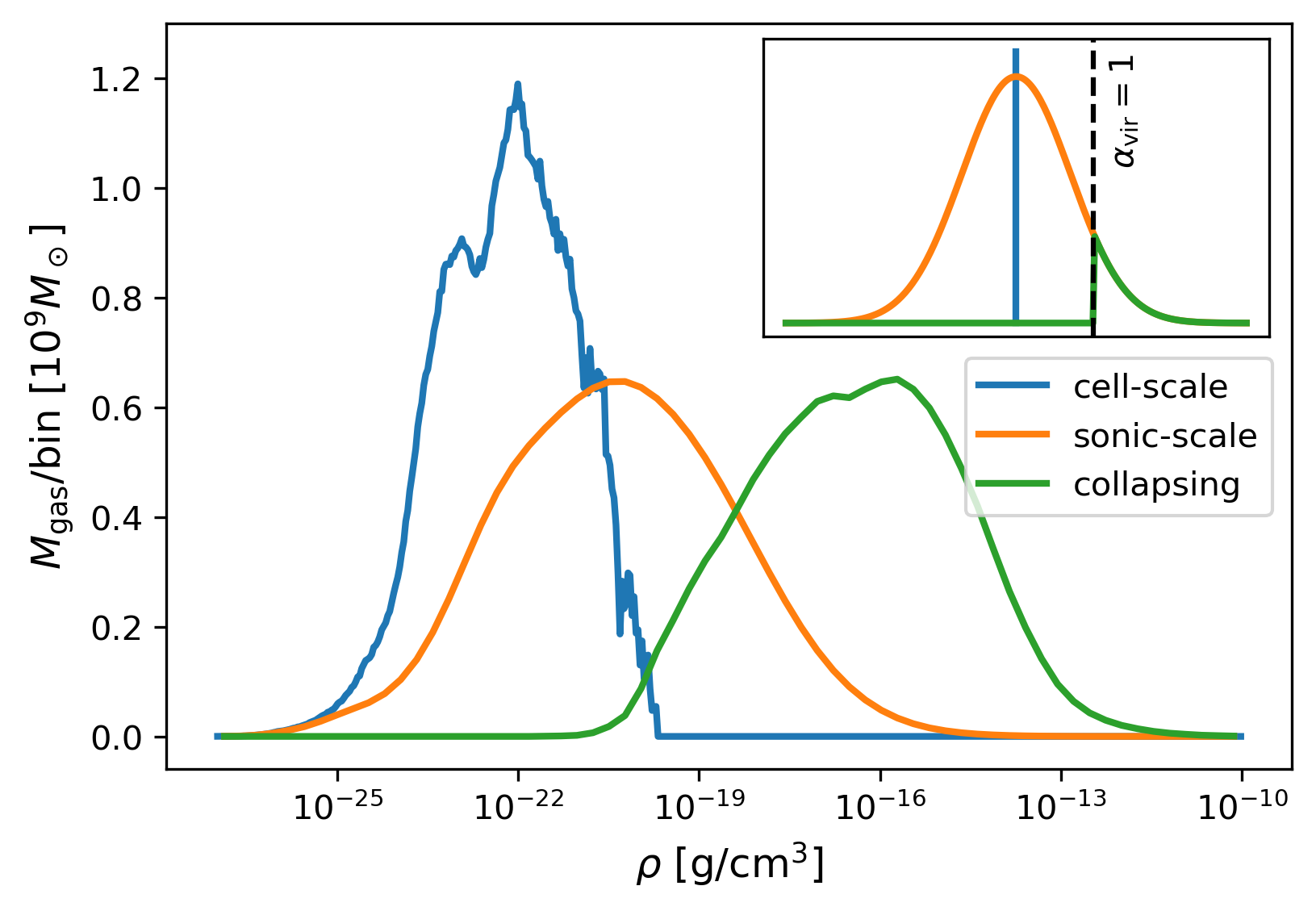
Figure 17: Histogram of the gas density in a box of sidelength $5~{}{\rm kpc}$ around the most massive galaxy in the fiducial simulation at $z=9$, weighted by gas mass. We compute the gas density using the raw cell value (blue), the subgrid density PDF given by the MFF model (orange), and the portion of the subgrid density PDF that is gravitationally unstable i.e. $\alpha_{\rm vir}<1$ (green). These histograms represent the cell-scale density distribution, the sonic-scale density distribution, and the density distribution of collapsing clouds respectively. The inset plot shows the convolution functions for clarity: a Dirac delta function for the cell-scale histogram (blue), a lognormal function for the sonic-scale histogram (orange), and a truncated lognormal function for the collapsing sonic-scale histogram (green).

Appendix F Spatial correlations of gas properties

In this section, we use 2-dimensional projections and slices to gain an intuition for the spatial correlation of gas properties. Spatial correlations are not captured by the PDFs analyzed in Section 3.4.

In Figure 18, we show slice plots of gas properties in the early feedback series. Regions of high density, low temperature, high Mach number, and low metallicity are spatially coincident. Likewise, regions of low density, high temperature, low Mach number, and high metallicity are spatially coincident. The low density regions tend to flow away from the galaxy.

As photoionization becomes more effective, the density field becomes more homogeneous, confirming our interpretation of the volume-weighted PDFs (Fig. 6). In noPhot, nearly all the gas mass is located in one central clump. In highPhot, the gas is distributed into multiple dense clumps and throughout the diffuse regions of the ISM. This helps explain why photoionization feedback leads to more SNe occurring in diffuse environments.

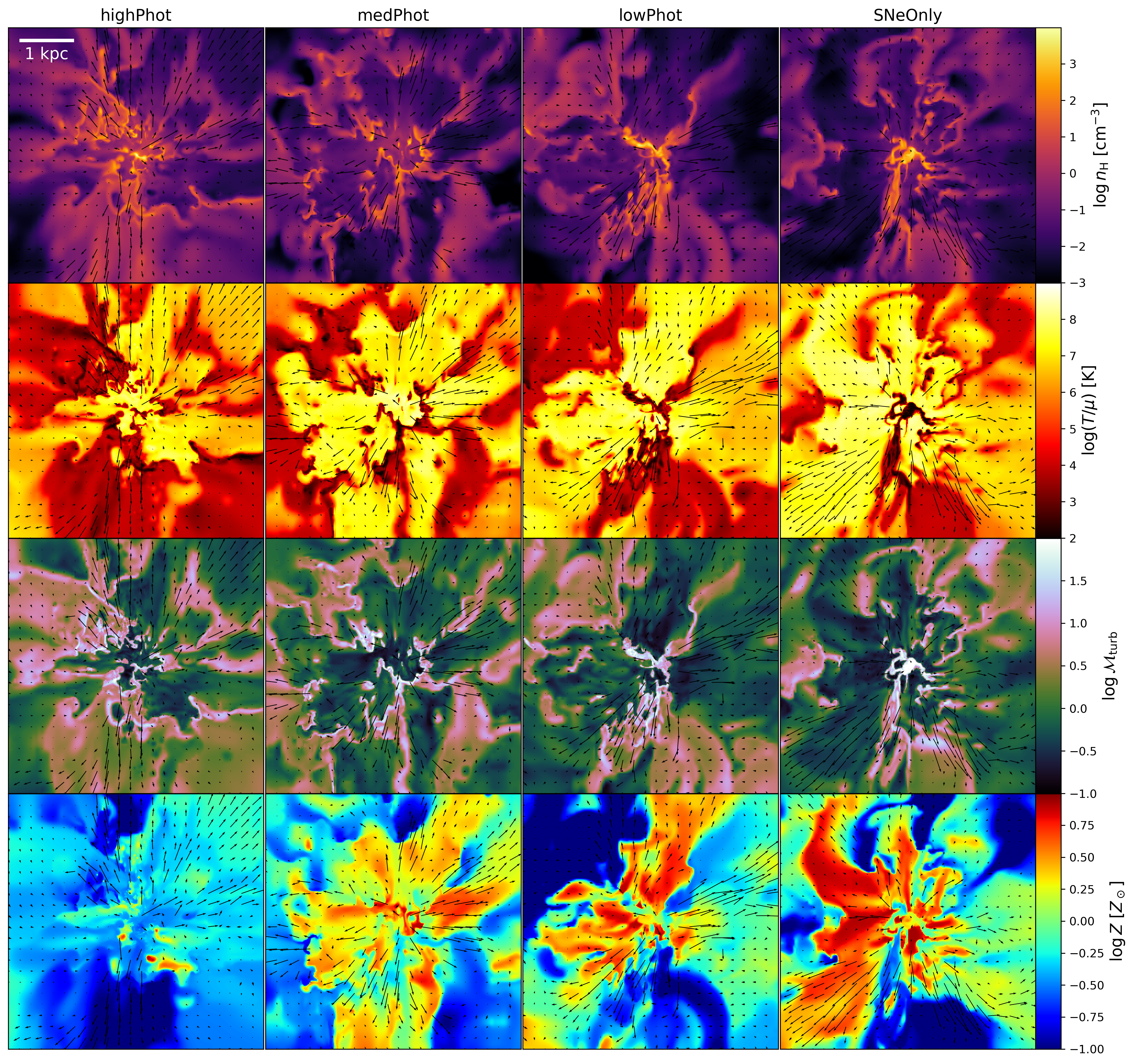
Figure 18: Logarithmic gas density (first row), temperature (second row), turbulent Mach number (third row), and metallicity (fourth row) in an $xy$ slice through the most massive galaxy in highPhot (first column), medPhot (second column), lowPhot (third column), and Nophot (fourth column) at $z=9$. We overlay arrows showing the direction and magnitude of the velocity field in each panel, with the bulk motion subtracted out.

It is difficult to predict a priori whether compressive or solenoidal forcing modes should dominate. On the one hand, the collapsing gas clouds and SN explosions associated with star formation drive compressive modes. This creates a positive feedback loop, because compressive forcing conditions enhance star formation. On the other hand, large-scale processes like accretion, mergers, and the differential rotation of a disc drive solenoidal modes, which suppress star formation. In varTurb, we capture these effects by computing the turbulence forcing parameter from the local velocity field.

In Figure 19, we show the velocity divergence and curl, proxies for the power in compressive and solenoidal forcing modes respectively, and the resulting forcing parameter in varTurb. The velocity field in regions near the galaxy is dominated by solenoidal motion, which should suppress star formation. However, the star formation history in varTurb is closer to compTurb than solTurb. This indicates that even though solenoidal forcing modes dominate the turbulence, a disproportionate fraction of star formation occurs in small pockets of compressive forcing.

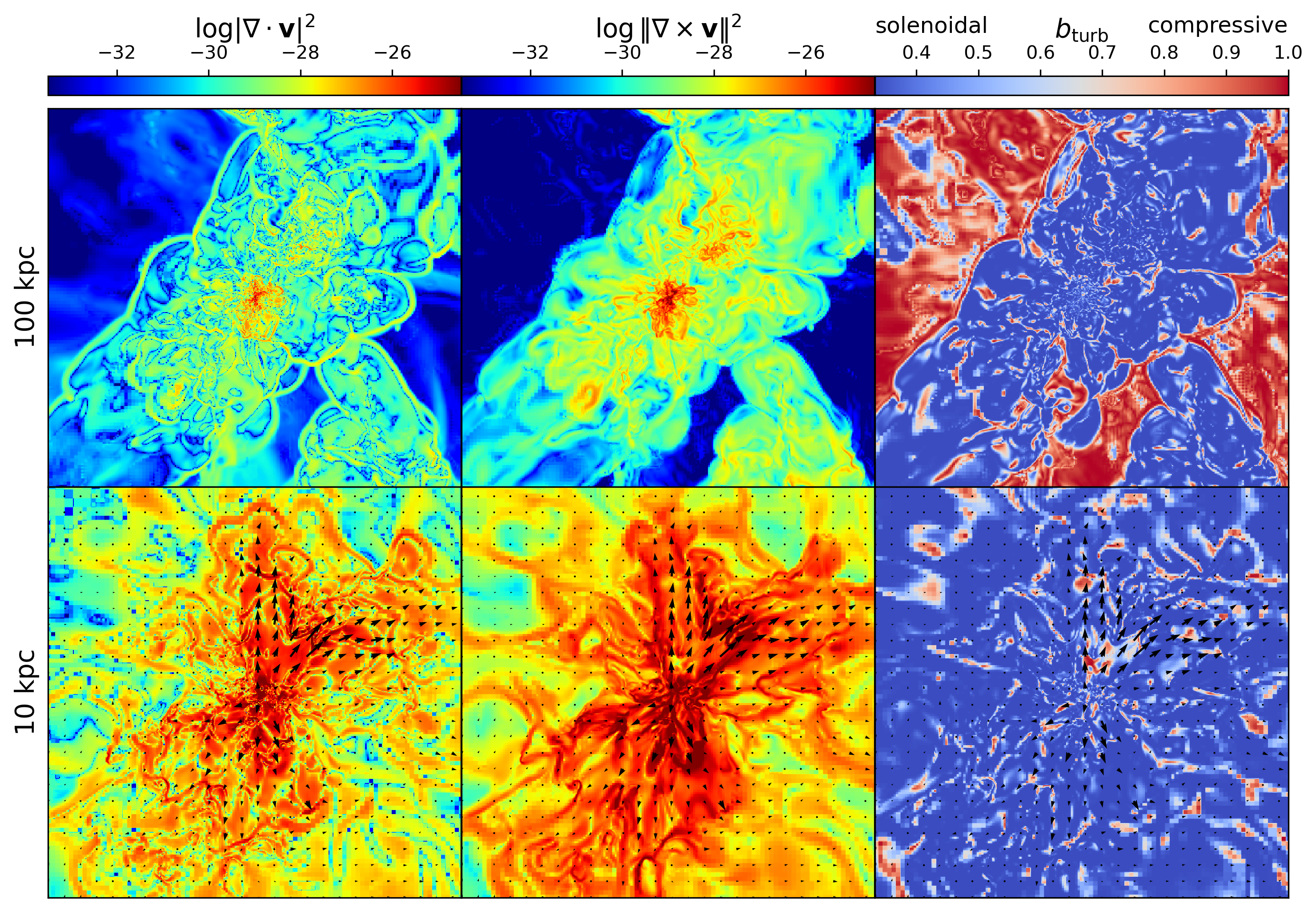
Figure 19: Logarithmic square of the velocity divergence (left column), square modulus of the velocity curl (middle column), and turbulence forcing parameter (right column) in an $xy$ slice through the most massive galaxy in the fiducial simulation at $z=9$ at a scale of $100~{}{\rm kpc}$ (top row) and $10~{}{\rm kpc}$ (bottom row). We overlay arrows showing the direction and magnitude of the velocity field in the bottom row. The square of the velocity divergence and velocity curl modulus are proxies for power in compressive and solenoidal forcing modes respectively.

Appendix G Column density PDF

The volume density PDF (Eq. 10) described by the MFF model can be related to the column density PDF, which can be directly measured from observations. Numerical simulations show that the column density PDF of supersonic turbulent gas is well-described by a log-normal distribution, similar to the volume density PDF (Federrath et al., 2010)

$$p(\eta)=\frac{1}{\sqrt{2\pi\sigma_{\eta}^{2}}}\exp\left[-\frac{(\eta-\overline{\eta})^{2}}{2\sigma_{\eta}^{2}}\right]$$ (68)

where $\eta=\ln(\Sigma/\overline{\Sigma})$ is the logarithmic surface density and $\sigma_{\eta}$ is the standard deviation of the logarithmic surface density in analogy to $s$ and $\sigma_{s}$ for the volume density PDF. We use $\eta$ to denote the logarithmic surface density for notational consistency with other work and rely on context to disambiguate the logarithmic surface density and outflow efficiency.

Equation 68 is supported observationally by measurements of column densities in the Perseus molecular cloud (Goodman et al., 2009). In general, the dispersion in the logarithmic column density distribution $\sigma_{\eta}$ is less than the dispersion in the logarithmic volume density distribution $\sigma_{s}$, because fluctuations are averaged out by integration along the line-of-sight.

The ratio $\sigma_{\eta}/\sigma_{s}$ decreases as the spectral slope of the density field decreases because the density field has less spatial correlation, so integration averages over more fluctuations. Previous work has shown that the spectral slope can be approximated by a power law in the Mach number (e.g. Seon, 2009).

Using that relationship, Seon (2012) show that the relationship between the two dispersions is well-approximated by a constant of proportionality $\sigma_{\eta}^{2}=A\sigma_{s}^{2}$, where $A$ depends only on the forcing parameter. For $b_{\rm turb}=1/3,0.5,1$, they find best fit values $A=0.2,0.24,0.38$ respectively.

We fit these data with a linear function using the least-squares method, which combined with Equation 12, yields

$$\sigma_{\eta}^{2}\approx(0.107b_{\rm turb}+0.272)\ln(1+b_{\rm turb}^{2}\mathcal{M}_{\rm turb}^{2})$$ (69)

Given the column density PDF $p(\Sigma)=p(\eta)/\Sigma$ and assuming a constant opacity $\kappa$, the optical depth PDF is simply $p(\tau)=\kappa p(\Sigma)$. The effective optical depth for a turbulent region can be estimated using a Rosseland-like averaging, which is equivalent to a PDF-weighted average over photon mean free path:

$$\tau_{\rm eff}=\left[\int\frac{\differential\tau p(\tau)}{\tau}\right]^{-1}=\frac{\kappa\overline{\Sigma}}{e^{\sigma_{\eta}^{2}}}$$ (70)

When applied to a cell in our simulations of size $\Delta x$, the mean surface density is $\overline{\Sigma}=\overline{\rho}\Delta x$.

Appendix H Breakdown of steady state

If the depletion time is long compared to the accretion timescale, then the SFR responds slowly to changes in the gas mass. In this case, the SFR passively reflects the current distribution of gas and is given by Equation 47. Dividing Equation 47 by the gas accretion rate to get the global SFE, we find

$$\epsilon_{\rm glob}=\frac{M_{\rm g}}{f_{\rm b}\dot{M}_{\rm acc}}\frac{f_{\rm sf}\epsilon_{\rm ff}}{\tau_{\rm ff}}$$ (71)

Consider the case where the local SFE is small or preventative feedback is weak such that the first term dominates in Equation 46. Then

$$f_{\rm sf}\approx\frac{1}{f_{\rm dyn}},\quad\tau_{\rm dep}\approx f_{\rm dyn}\frac{\tau_{\rm ff}}{\epsilon_{\rm ff}}$$ (72)

and

$$\epsilon_{\rm glob}\approx\frac{M_{\rm gas}}{f_{\rm b}\dot{M}_{\rm acc}\tau_{\rm ff}}\frac{\epsilon_{\rm ff}}{f_{\rm dyn}}$$ (73)

In this case, the global SFE is proportional to the local SFE, so the galaxy is not self-regulated. (Semenov et al., 2018) call this the dynamics-regulation regime.

Now consider the case where the local SFE is large or preventative feedback is weak such that the second term dominates in Equation 46. Then

$$f_{\rm sf}\approx\frac{\tau_{\rm ff}}{\tau_{\rm cool}}\frac{1}{(1+\mu)\epsilon_{\rm ff}},\quad\tau_{\rm dep}\approx(1+\mu)\tau_{\rm cool}$$ (74)

and

$$\epsilon_{\rm glob}\approx\frac{M_{\rm gas}}{f_{\rm b}\dot{M}_{\rm acc}\tau_{\rm cool}}\frac{1}{1+\mu}$$ (75)

Similar to when steady state applies, the global SFE is independent of the local SFE, so the galaxy is self-regulated. However, rather than ejective feedback, the global SFE is regulated by preventative feedback. (Semenov et al., 2018) call this the feedback-regulation regime.

When steady state applies, the galaxy is always self-regulated. When steady state does not apply, the galaxy is only self-regulated if the local SFE satisfies

$$\epsilon_{\rm ff}\gg\frac{\tau_{\rm ff}}{\tau_{\rm cool}}\frac{f_{\rm dyn}}{1+\mu}$$ (76)

Essentially, the local SFE must be large enough for preventative feedback to remove gas from the star-forming state faster than it is supplied by cooling and collapse.

References

- Agertz et al. (2013) Agertz O., Kravtsov A. V., Leitner S. N., Gnedin N. Y., 2013, ApJ, 770, 25
- Alcalde Pampliega et al. (2019) Alcalde Pampliega B., et al., 2019, ApJ, 876, 135
- Andalman & Teyssier (2024) Andalman Z. L., Teyssier R., 2024, Star Formation Histories of Simulated Massive Galaxies at Cosmic Dawn, 10.34770/v56h-ps15
- André et al. (2010) André P., et al., 2010, A&A, 518, L102
- Antwi-Danso et al. (2023) Antwi-Danso J., et al., 2023, arXiv e-prints, p. arXiv:2307.09590
- Aubert & Teyssier (2010) Aubert D., Teyssier R., 2010, ApJ, 724, 244
- Audit & Hennebelle (2010) Audit E., Hennebelle P., 2010, A&A, 511, A76
- Beattie et al. (2019) Beattie J. R., Federrath C., Klessen R. S., Schneider N., 2019, MNRAS, 488, 2493
- Beattie et al. (2022) Beattie J. R., Mocz P., Federrath C., Klessen R. S., 2022, MNRAS, 517, 5003
- Bleuler & Teyssier (2014) Bleuler A., Teyssier R., 2014, MNRAS, 445, 4015
- Boylan-Kolchin (2023) Boylan-Kolchin M., 2023, Nature Astronomy, 7, 731
- Bressert et al. (2010) Bressert E., et al., 2010, MNRAS, 409, L54
- Bromm & Loeb (2003) Bromm V., Loeb A., 2003, Nature, 425, 812
- Brucy et al. (2024) Brucy N., Hennebelle P., Colman T., Klessen R. S., Le Yhuelic C., 2024, arXiv e-prints, p. arXiv:2404.17374
- Bullock et al. (2001) Bullock J. S., Dekel A., Kolatt T. S., Kravtsov A. V., Klypin A. A., Porciani C., Primack J. R., 2001, ApJ, 555, 240
- Cameron et al. (2023) Cameron A. J., Katz H., Witten C., Saxena A., Laporte N., Bunker A. J., 2023, arXiv e-prints, p. arXiv:2311.02051
- Caplar & Tacchella (2019) Caplar N., Tacchella S., 2019, MNRAS, 487, 3845
- Carnall et al. (2018) Carnall A. C., McLure R. J., Dunlop J. S., Davé R., 2018, MNRAS, 480, 4379
- Carnall et al. (2023) Carnall A. C., et al., 2023, Nature, 619, 716
- Carnall et al. (2024) Carnall A. C., et al., 2024, arXiv e-prints, p. arXiv:2405.02242
- Carniani et al. (2024) Carniani S., et al., 2024, arXiv e-prints, p. arXiv:2405.18485
- Casey et al. (2023) Casey C. M., et al., 2023, ApJ, 954, 31
- Casey et al. (2024) Casey C. M., et al., 2024, ApJ, 965, 98
- Castaing (1996) Castaing B., 1996, Journal de Physique II, 6, 105
- Chabrier (2003) Chabrier G., 2003, PASP, 115, 763
- Choban et al. (2022) Choban C. R., Kereš D., Hopkins P. F., Sandstrom K. M., Hayward C. C., Faucher-Giguère C.-A., 2022, MNRAS, 514, 4506
- Conroy & Gunn (2010) Conroy C., Gunn J. E., 2010, ApJ, 712, 833
- Conroy et al. (2009) Conroy C., Gunn J. E., White M., 2009, ApJ, 699, 486
- Correa et al. (2015) Correa C. A., Wyithe J. S. B., Schaye J., Duffy A. R., 2015, MNRAS, 450, 1514
- Danovich et al. (2015) Danovich M., Dekel A., Hahn O., Ceverino D., Primack J., 2015, MNRAS, 449, 2087
- Dekel & Mandelker (2014) Dekel A., Mandelker N., 2014, MNRAS, 444, 2071
- Dekel et al. (2009) Dekel A., Sari R., Ceverino D., 2009, ApJ, 703, 785
- Dekel et al. (2013) Dekel A., Zolotov A., Tweed D., Cacciato M., Ceverino D., Primack J. R., 2013, MNRAS, 435, 999
- Dekel et al. (2023) Dekel A., Sarkar K. C., Birnboim Y., Mandelker N., Li Z., 2023, MNRAS, 523, 3201
- Diemer (2018) Diemer B., 2018, ApJS, 239, 35
- Draine (2011) Draine B. T., 2011, Physics of the Interstellar and Intergalactic Medium. Princeton University Press
- Eisenstein et al. (2023) Eisenstein D. J., et al., 2023, arXiv e-prints, p. arXiv:2306.02465
- Elmegreen et al. (2007) Elmegreen D. M., Elmegreen B. G., Ravindranath S., Coe D. A., 2007, ApJ, 658, 763
- Faucher-Giguère et al. (2013) Faucher-Giguère C.-A., Quataert E., Hopkins P. F., 2013, MNRAS, 433, 1970